Download MQGPS User`s Manual

Users Manual
Covers VEQTR™ AND MQGPS MODELS
(QUANTUM™, QUANTUM™ WIFI V2, QUANTUM
DOT™, HIDEF™, TRAQR™, and 5HZ™)
© Copyright 2009 MaxQData, LLC
2
MaxQData, LLC
Windows Desktop and Windows Mobile Software
END USER LICENSE AGREEMENT
NOTICE: THIS IS A LEGAL AGREEMENT BETWEEN YOU AND MAXQDATA, LLC. YOU MUST READ
AND ACCEPT ALL OF THE TERMS OF THIS END USER LICENSE AGREEMENT IN ORDER TO BE
LICENSED TO USE THE ACCOMPANYING SOFTWARE. USAGE OF ANY COMPONENT OF THE
ACCOMPANYING SOFTWARE, OR INSTALLATION OF THE ACCOMPANYING SOFTWARE ON A
COMPUTER, OR DOWNLOADING THE SOFTWARE INDICATES YOUR ACCEPTANCE OF AND BINDS
YOU TO ALL THE TERMS OF THIS AGREEMENT. READ THIS AGREEMENT CAREFULLY. IF YOU ARE
NOT WILLING TO ACCEPT THE TERMS OF THIS AGREEMENT, DO NOT DOWNLOAD OR INSTALL OR
USE THE SOFTWARE.
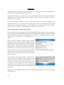
This MaxQData, LLC ("MaxQData") End User License Agreement ("EULA") covers the accompanying software
products and related written materials and images, including but not limited to Chart, Flight, gCal, Setup, Codes,
MQGPS-Tracker Manager, sensor drivers, related .DLLs, and other related software and documentation
(collectively, "Software"), designed to work with related MaxQData hardware products or compatible products
from third parties ("Hardware"). This End User License Agreement also covers upgrades, patches, bug fixes, or
documentation or utility software, related to said software product or written materials or images, that are
distributed without an accompanying EULA. You must agree to use any Hardware according to all terms and
conditions in this EULA in order be licensed to use the Software.
1. Intellectual Property
MaxQData owns intellectual property rights in the Software and Hardware, including but not limited to
Copyright, Patent, Look and Feel, Trade Dress, Trademark, and Trade Secret rights. These rights are protected
by U.S. and international laws and treaties. You agree not to violate these intellectual property rights. You agree
not to copy the Software except as explicitly allowed herein. You agree not to reverse engineer the Software or
Hardware, including data file formats and APIs.
2. Terms and Fees
You are not licensed until you have accepted all the terms and conditions of this EULA and paid the appropriate
license and/or purchase fees for the Software and/or Hardware to MaxQData or its authorized distributor or
reseller.
3. Installation
In the absence of a separate specific license agreement superseding this section, you are permitted to install the
Software on an unlimited number of computers, as long as you own, lease, or rent each computer. You may be
required to purchase unlock or registration codes for each separate installation. You are not permitted to install
the Software on computers you do not own, lease, or rent, except when you are acting as an agent of the owner
and the owner is licensed under this EULA. You must remove the Software before the computer on which it is
installed passes from your control.
4. Use
3
You are permitted to use the Software and Hardware so long as your use of the Software and Hardware does not
violate any laws, including but not limited to traffic laws and noise ordinances. You are permitted to use the
Software and Hardware only when exercising due caution, when using appropriate safety equipment, and
under circumstances that present no unusual or unexpected risk to life, limb, or property. Usage and licensing
restrictions mentioned elsewhere in this EULA supersede the provisions of this section.
5. Third Party Use
You agree that third-party use of any Software licensed to you shall be on a short-term basis (e.g. for a racing
event; for a demonstration; for instructional purposes; where the scope of use is limited in duration to a racing
event or less and the Software returns to your possession and control afterwards) and only when you are present
and aware of that party's actions. Refer to section "Indemnification" for other relevant terms and conditions.
6. Suggestions
You grant MaxQData a fully-paid-up, perpetual, unrestricted, transferrable, irrevocable license to any
recommendations, improvements, new product ideas, designs, copyrighted material, or patentable methods you
transmit to MaxQData or post on any forum or Wiki owned or managed by MaxQData, whether solicited or
unsolicited, for use in its present or future products, services, or business methods.
7. Data
You grant MaxQData a fully-paid-up, perpetual, unrestricted, transferrable, irrevocable license to any flight
recordings, data files, telemetry data, images, video, or debug logs (collectively "Data"), related to or deriving
from your use of the Software or Hardware, which you transmit to MaxQData, or post on any forum or Wiki
owned or managed by MaxQData, whether solicited or unsolicited.
8. Indemnification
You agree to indemnify and hold harmless MaxQData for any claim against it regarding all: a) injuries or
damages occurring during or resulting from your use of the Hardware and/or the Software, and b) injuries or
damages occurring during or resulting from third party use of Hardware owned by you and/or Software
licensed to you. You agree this indemnification shall hold if your use of the Hardware and/or Software is not
properly licensed or is in violation of other terms of this EULA. You agree this indemnification shall hold under
any circumstances and in any place including but not limited to injuries or damages occurring while racing,
while on public or private roads or property, while on a body of water or while airborne, and even when such
injuries or damages are claimed or proven to have resulted from correct, incorrect, unexpected, distracting, or
erroneous operation or inoperation of the Software or Hardware, and even when such injuries or damages were
foreseeable or not foreseeable by you or by MaxQData, and even when an agent of MaxQData was present at the
time of the injuries or damages, and even when an agent of MaxQData was in control of or co-driving or riding
with the vehicle used at the time of the injuries or damages. You agree to indemnify and hold harmless
MaxQData for any claim against it by you or by third parties for intellectual property you transmitted to
MaxQData covered by section "Suggestions" or section "Data".
9. Disclaimer of Warranties
MaxQData provides the Software and Hardware AS IS AND WITH ALL FAULTS. MAXQDATA MAKES NO
WARRANTIES, EXPRESS OR IMPLIED OR STATUTORY, AS TO NONINFRINGEMENT OF THIRD PARTY
RIGHTS, MERCHANTABILITY, ACCURACY, SAFETY, LACK OF NEGLIGENCE, LACK OF WORKMANLIKE
EFFORT, OR FITNESS FOR ANY PARTICULAR PURPOSE. IN NO EVENT WILL MAXQDATA BE LIABLE TO
4
YOU FOR ANY CONSEQUENTIAL, INCIDENTAL OR SPECIAL DAMAGES, INCLUDING ANY LOST
PROFITS OR LOST SAVINGS, TOWING CHARGES, RACING DAMAGES, EMISSIONS-RELATED FAILURES
OR VIOLATIONS, OR TRAFFIC TICKETS, EVEN IF A MAXQDATA REPRESENTATIVE HAS BEEN ADVISED
OF THE POSSIBILITY OF SUCH DAMAGES, OR THE POSSIBILITY OF SUCH DAMAGES WAS
FORESEEABLE BY MAXQDATA, OR FOR ANY CLAIM BY ANY THIRD PARTY. THE ENTIRE RISK AS TO
THE QUALITY OF THE SOFTWARE, ITS PERFORMANCE, SIDE EFFECTS, AND FORSEEN OR UNFORSEEN
CONSEQUENCES OF USE, REMAINS WITH YOU. Some states or jurisdictions do not allow the exclusion or
limitation of incidental, consequential or special damages, or the exclusion of implied warranties or limitations
on how long an implied warranty may last, so the above limitations may not apply to you. To the extent
permissible, any implied warranties are limited to ninety (90) days.
10. Disclaimer of Accuracy and Reliability and Usage Restrictions
THE ACCURACY OF THE MEASUREMENTS AND ESTIMATES PRODUCED BY THE SOFTWARE AND
HARDWARE IS NOT GUARANTEED. YOU ARE NOT LICENSED TO USE THE SOFTWARE OR
HARDWARE IN SITUATIONS WHERE INACCURATE MEASUREMENTS OR ESTIMATES COULD RESULT
IN INJURIES OR DAMAGES TO ANY PARTY OR VIOLATIONS OF THE LAW. THE RELIABILITY OF THE
SOFTWARE AND HARDWARE IS NOT GUARANTEED. YOU ARE NOT LICENSED TO USE THE
SOFTWARE OR HARDWARE IN SITUATIONS WHERE FAILURE OF THE SOFTWARE OR HARDWARE
COULD RESULT IN INJURIES OR DAMAGES TO ANY PARTY OR VIOLATIONS OF THE LAW. YOU ARE
NOT LICENSED TO USE THE SOFTWARE OR HARDWARE IN ANY LIFE SUPPORT OR SAFETY SYSTEM.
YOU ARE NOT LICENSED TO USE THE SOFTWARE OR HARDWARE TO CONTROL A MOVING VEHICLE.
YOU ARE NOT LICENSED TO USE THE SOFTWARE OR HARDWARE IN ANY SITUATION OR UNDER
ANY CIRCUMSTANCES WHERE THE SOFTWARE OR HARDWARE OR MEASUREMENTS AND
ESTIMATES GENERATED BY THEM IS USED, IN WHOLE OR IN PART, AS A SUBSTITUTE FOR HUMAN
JUDGMENT OR HUMAN ACTION. YOU ARE NOT LICENSED TO USE THE SOFTWARE OR HARDWARE
IN ANY SITUATION OR UNDER ANY CIRCUMSTANCES WHERE THE USE OF THE SOFTWARE OR
HARDWARE, EVEN IF ACCURACY AND RELIABILITY ARE NOT AT ISSUE, COULD RESULT IN INJURIES
OR DAMAGES TO ANY PARTY OR VIOLATIONS OF THE LAW.
11. Termination
Termination is automatic at the time you violate any of the provisions in this EULA. MaxQData may terminate
this EULA at any time with or without cause, and with or without refunding any license fees. You may
terminate this EULA at any time, with or without cause, by destroying all copies of the Software and notifying
MaxQData. In the event of termination, you agree to destroy all copies of the Software. The provisions of
section "Intellectual Property", section "Suggestions", section "Data", section "Indemnification", section
"Disclaimer of Warranties", and section "Governing Law" shall survive termination.
12. Governing Law
This EULA is governed by the laws of the State of Washington.
13. Version, Supersession, Other Provisions
This EULA is version 5, revised February 28, 2009, and supersedes all previous EULAs upon installation or
download of any accompanying Software. If any provision of this EULA shall be held to be invalid,
unenforceable, or void, the remainder of this EULA shall remain in full force and effect.
5
Cautions, Warnings, and Disclaimers ........................................................................................................... 11
Battery Safety – Lithium-based Batteries ...................................................................................................11
Measurement Errors .....................................................................................................................................11
Use on Public Roads .....................................................................................................................................11
Survivability of Hard Drives In-Vehicle ....................................................................................................12
Quantum™ Quickstart Guide – Standalone Operation ............................................................................ 14
Quantum™ Quickstart Guide – Connected Operation – Bluetooth Models ......................................... 18
Quantum™ and Quantum Dot™ Quickstart Guide – Connected Operation – WiFi Models ............ 23
MQGPS-5Hz™ and MQGPS-HiDef™ Quickstart Guide ........................................................................ 26
TraQr™ Quickstart Guide .............................................................................................................................. 32
Mounting Considerations ............................................................................................................................... 35
MQGPS ...........................................................................................................................................................35
Pocket PC/iPhone ..........................................................................................................................................35
Laptop ............................................................................................................................................................36
Using the Quantum – Standalone Operation .............................................................................................. 37
Method of Operation ....................................................................................................................................37
Setup ...............................................................................................................................................................37
Flight Recording Trigger – Quantum Internal Trigger ............................................................................38
Flight Recording Trigger – Flight ...............................................................................................................39
Using the Quantum – Connected Operation ............................................................................................... 40
Using the TraQr ................................................................................................................................................ 41
Method of Operation ....................................................................................................................................41
Setup ...............................................................................................................................................................41
TraQr Manager – General Tab ....................................................................................................................42
Advanced Tab ...............................................................................................................................................43
Download Process ........................................................................................................................................44
Flight Recording Trigger..............................................................................................................................45
Bluetooth Download ....................................................................................................................................46
Using Flight ....................................................................................................................................................... 47
Initial Configuration .....................................................................................................................................47
Display Dashboard .......................................................................................................................................49
6
Display Graphs ............................................................................................................................................. 50
Starting a Flight Recording – Automatic Flight Recording Trigger....................................................... 53
Starting a Flight Recording – Screen Tap .................................................................................................. 53
Starting a Flight Recording – Other Methods ........................................................................................... 54
Changing the Default Filename Prefix ....................................................................................................... 55
Mulitple Driver Support .............................................................................................................................. 55
Preopened Flight Recording File ................................................................................................................ 56
The Preopened Flight Recording File and Pit Stops ................................................................................ 56
Timeslips ........................................................................................................................................................ 57
Launch Chart at End of Run........................................................................................................................ 57
Display Report .............................................................................................................................................. 57
Course Walk Beacons ................................................................................................................................... 57
Using Chart ........................................................................................................................................................ 59
User Interface ................................................................................................................................................ 61
Viewing Data – Simple Corner Analysis ................................................................................................... 64
Data Smoothing ............................................................................................................................................ 66
Landscape Mode User Interface ................................................................................................................. 68
Using GPS Beacons ....................................................................................................................................... 68
Example – Placing Beacons ......................................................................................................................... 69
Adding Beacons ............................................................................................................................................ 71
Exporting Beacons ........................................................................................................................................ 73
Importing Beacons ........................................................................................................................................ 73
Viewing the List of Lap and Segment Times ............................................................................................ 74
Comparing Two Laps .................................................................................................................................. 75
Determining Time Lost/Gained .................................................................................................................. 78
Comparing Two Laps with Qview™ ......................................................................................................... 80
Zooming in on Qview™ .............................................................................................................................. 82
Comparing Lines .......................................................................................................................................... 83
Showing Lap and Segment Timing ............................................................................................................ 84
Plot by Time vs. Plot by Distance ............................................................................................................... 85
g-g Plot ........................................................................................................................................................... 85
Show Grid ...................................................................................................................................................... 87
Align to Start of Run..................................................................................................................................... 87
Set zero time .................................................................................................................................................. 87
Play ................................................................................................................................................................. 87
Show Yaw Path, Show g Path ..................................................................................................................... 87
Copy [t..tA] and Copy [t..tB] ....................................................................................................................... 88
Manual Beacon Editing in Chart ................................................................................................................ 88
Comparing Laps from Different Files ........................................................................................................ 88
Exporting Data .............................................................................................................................................. 89
Qview Report ................................................................................................................................................ 90
Loading a CSV File ....................................................................................................................................... 93
Modifying the CSV Parse Configuration ................................................................................................... 93
Course Walk Beacons and Cones ............................................................................................................... 95
7
Slide map B ....................................................................................................................................................96
Enable video load (PC only) ........................................................................................................................96
Produce video overlay (PC only) ................................................................................................................96
Using Setup........................................................................................................................................................ 97
Calibration and Sensors ...............................................................................................................................97
Lap Time Beacons .........................................................................................................................................99
Saving the Calibration ..................................................................................................................................99
Serial Communications ................................................................................................................................99
MQ Module Configuration........................................................................................................................100
Email and SMS Text Message Telemetry .................................................................................................100
Advanced Options ......................................................................................................................................101
Camera Capture Settings ...........................................................................................................................102
VeQtr™ Video Capture Features ................................................................................................................. 103
Video Capture Basic Concepts ..................................................................................................................103
Camera Capture Setup ...............................................................................................................................104
Start and Stop Capturing ...........................................................................................................................108
Video Capture and the Flight Recording Trigger ...................................................................................108
Video Sync Sensor.......................................................................................................................................108
Video capture output files .........................................................................................................................109
Notebook/PC Requirements and Usage Notes .......................................................................................109
USB Camera Requirements and Usage Notes ........................................................................................110
Bypassing WMV Compression for Advanced Users .............................................................................112
VeQtr™ Video Playback and Overlay Generation in Chart .................................................................. 114
Loading a Video File...................................................................................................................................114
Synchronizing Video and Data .................................................................................................................116
Produce Video Overlay ..............................................................................................................................116
Transcoding .................................................................................................................................................119
Initialization .................................................................................................................................................119
Exporting......................................................................................................................................................119
Direct upload to YouTube .........................................................................................................................120
Using the MQGPS for Road Racing ............................................................................................................ 122
Racing Type .................................................................................................................................................122
Pocket PC Mounting...................................................................................................................................122
Finding a Racing Buddy ............................................................................................................................122
Setting Beacons ............................................................................................................................................122
Showing Real-Time Lap and Segment Times .........................................................................................122
Showing Lap Time without using Beacons .............................................................................................125
MQGPS and Pocket PC Power Usage ......................................................................................................125
8
Road Racing Data Analysis ....................................................................................................................... 126
Using the MQGPS for Autocrossing ........................................................................................................... 128
Racing Type ................................................................................................................................................. 128
Finding a Racing Buddy ............................................................................................................................ 128
Flight Recording Trigger ........................................................................................................................... 128
Flight Recording Trigger vs Manual Trigger .......................................................................................... 129
Walking the Course and Placing Beacons ............................................................................................... 129
Back-to-Back Runs ...................................................................................................................................... 129
Stopping after your Run ............................................................................................................................ 129
MQGPS and Pocket PC Power Usage ...................................................................................................... 130
Real-time Segment Time Display ............................................................................................................. 130
Autocrossing Data Analysis ...................................................................................................................... 130
Using the MQGPS for Drag Racing ............................................................................................................ 132
Racing Type ................................................................................................................................................. 132
Log Options in Flight ................................................................................................................................. 132
GPS Beacons ................................................................................................................................................ 132
Recording Your Run ................................................................................................................................... 132
Timeslip Information ................................................................................................................................. 133
Accuracy ...................................................................................................................................................... 136
Telemetry ......................................................................................................................................................... 138
SMS Text Messaging of Lap and Segment Times ................................................................................... 138
Email of Flight Recording Files ................................................................................................................. 139
Generating a Google Earth Satellite Plot ................................................................................................... 141
Sensor Reference ............................................................................................................................................ 142
Flight recording trigger .............................................................................................................................. 142
Standard GPS values .................................................................................................................................. 142
GPS Beacon timestamp .............................................................................................................................. 143
GPS Distance ............................................................................................................................................... 144
GPS Time Since Last Here ......................................................................................................................... 145
GPS LongG .................................................................................................................................................. 145
GPS Jerk ....................................................................................................................................................... 146
GPS LatG ...................................................................................................................................................... 146
GPS Power ratio .......................................................................................................................................... 146
GPS Road power ......................................................................................................................................... 147
GPS Turn radius.......................................................................................................................................... 147
GPS VertG .................................................................................................................................................... 147
Sensors for Quantum WiFi V2 .................................................................................................................. 148
9
Roll Rate Pitch Rate Yaw Rate ...................................................................................................................148
Drift ...............................................................................................................................................................148
This value estimates how far the car ‚steps out‛ or ‚pushes‛ during cornering. A value
significantly above 1.0 indicates oversteer. A value much below 1.0 indicates understeer. ...........148
Lean Angle ...................................................................................................................................................148
Applies to motorcycles only when MotionModel,1 is set in quantum_config.txt. This value
estimates the lean angle of the motorcycle. .............................................................................................148
Voice Output ................................................................................................................................................... 150
Quantum™ Tips and Tricks ......................................................................................................................... 151
Quantum™ Configuration ............................................................................................................................ 152
VeQtr™ Tips and Tricks ............................................................................................................................... 159
VeQtr™ DIY Setup and Configuration – Windows XP ........................................................................... 160
VeQtr™ DIY Setup and Configuration – Windows 7 .............................................................................. 162
About MaxQData™ ........................................................................................................................................ 164
Revision 19
10
Cautions, Warnings, and Disclaimers
Any activity involving moving vehicles may be dangerous to health, life, or property, even when all
the rules and safety procedures are followed. MaxQData disclaims responsibility for anything
adverse that happens while you use a MaxQData product. Your use of the product indicates your
assent to this disclaimer. Please review the End User License Agreement for more details.
Battery Safety – Lithium-based Batteries
Most modern Pocket PCs, Smartphones, PDAs, and laptop or notebook computers employ lithium
battery technology. MaxQData does not manufacture these batteries. Given the wide range of
potential applications, MaxQData does not certify the appropriateness or safety of the use of lithiumbased batteries in moving vehicles or racing applications. The responsibility for making this
determination rests solely with the user. Please pay attention to any cautions or warnings from the
equipment manufacturer about the temperature limitations of the lithium-based batteries used in
your notebook computer. Most lithium-based batteries contain internal safeguards, but even so
extreme heat, manufacturing defects, or physical damage (e.g. in the event of a crash or accident)
could cause a battery to ignite and burn forcefully. Be sure any fire suppression system in the
vehicle is suitable for extinguishing this type of fire. Never use a water-based fire extinguisher to
put out an electrical or lithium fire. Do not use any battery that has been physically damaged.
Concerns about lithium battery safety can also be addressed simply by removing the battery pack
and running off of a car power adapter or an external non-lithium battery pack.
Battery Safety – Alkaline, NiMH, NiCd, and other battery types
Please be sure to respect all manufacturer’s safety warnings and to use such batteries only under
environmental conditions for which they are approved.
Instrumentation Only
MaxQData systems record and display information about the motion of the vehicle. They do not tell
the driver ‚what to do‛, only ‚what he did‛. They do not control the vehicle. The driver is solely
responsible for interpreting the information and applying the knowledge in a safe and legal manner.
Measurement Errors
All measuring systems are subject to measurement errors. Use caution and common sense when
interpreting data collected by a measuring system. Never use a MaxQData system for the purpose of
controlling a moving vehicle.
Use on Public Roads
Please be sure to comply with all laws regarding your use and operation of a MaxQData system. Do
not use the system in violation of traffic laws. Some US States prohibit or restrict the use of cell
11
phones while driving. Some US States prohibit the use of suction cup mounts on windshields. There
may be other prohibitions or restrictions in different States and Countries.
Survivability of Hard Drives In-Vehicle
Hard disk drives using rotating media are susceptible to permanent damage due to vibration and
shock. This can result in the loss of data or even prevent the computer from booting. It is the user’s
sole responsibility to determine whether a hard disk drive is suitable for use in their vehicle and the
environment in which it will be used. Use common sense and shock-mount the computer
appropriately to help minimize the risk. Solid-State Disks (‚SSDs‛) are strongly suggested for
vehicles with very harsh rides, especially purpose-built racecars. Users with extreme requirements
should contact MaxQData for ruggedized PC options.
12
13
Quantum™ Quickstart Guide – Standalone Operation
Thank you for purchasing a MaxQData™ MQGPS™ system. If you have any problems getting
started, you can send email to [email protected].
PLEASE NOTE – IF YOU PURCHASED YOUR QUANTUM AS PART OF A COMPLETE SYSTEM
FROM MAXQDATA, DO NOT FOLLOW THIS QUICKSTART GUIDE. THE SYSTEM IS ALREADY
SET UP FOR YOU.
‚Standalone‛ operation means that the Quantum™ will capture data directly to its internal memory,
and later the user will extract the data to a Windows laptop PC for analysis. If you wish to use
‚Connected‛ operation where the Quantum sends data to a Pocket PC or laptop PC in real time via
Bluetooth, please refer to the Quantum Quickstart Guide for ‚Connected Operation‛.
Battery Charging – Models with Built-In Battery
The Quantum charges from any USB port. Use the included USB-to-mini USB cable for charging.
The status light will glow red while the battery is charging and will turn off when the battery is done
charging. Maximum charge time is typically 2-3 hours. The battery is internal and should last the life
of the system but can be replaced by the user if necessary – contact MaxQData for details. An
optional double capacity battery is available. Run time is about 8 hours. Be sure to switch off the
Quantum when not in use.
Batteries – Models that use AA batteries
Run time with rechargeable NiMH batteries is about 5 hours. Alkaline batteries should last about
half that time. Disposable lithium batteries should last about double that time. Be sure to switch off
the Quantum when not in use. For endurance racing or other applications requiring continuous
power, you can omit the batteries and connect a 2.5V-3.0V, 500 mA, regulated and filtered power
supply.
Status Light – Models with Built-In Battery




Red means charging
Flashing green means data is being received from the GPS satellites. This flash will turn into
a shorter, quicker flash once satellite lock is achieved.
Flashing blue means data is being transmitted over Bluetooth.
When the unit is turned on, the blue and green lights both turn on, then the blue light turns
off, and then the green light turns off. The green light will then begin flashing when GPS
data is received.
Status Lights – Models that use AA batteries

14
Red slow flash: power is on






Red fast flash: low battery
Solid red: Standby
Green slow flash: GPS searching, unit not ready for use
Green fast flash: GPS locked, unit is ready for use
Blue slow flash: Wireless is connected
Blue fast flash: Transmitting data
Step 1 – Software Download and Installation – Laptop/Desktop
Download the latest software from the MaxQData website. You will need the file labeled ‚PC
Complete System Software‛, not the one labeled ‚PC Chart Only‛. The name of the file will be
similar to ‚MaxQData 34b PC Software.exe‛. Download the file to your laptop and double-click on it
to run it. Do not install the ‚TraQr Manager‛ application. Also do not install any MQGPS drivers.
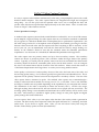
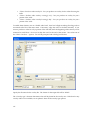
Step 2 – Software Setup for Standalone Operation
Run MaxQData Setup and configure the software according to the following settings:
Settings > Serial Port Settings:









‚MQ Port‛ must be ‚NONE‛ (all caps, no quotes).
‚Is Bluetooth‛ under ‚MQ Port‛ does not matter.
‚MQ Baud Rate‛ does not matter
‚Delay Bluetooth Init‛ should be unchecked.
‚GPS Port‛ must be ‚TXT‛ (all caps, no quotes)
‚Is Bluetooth‛ under ‚GPS Port‛ should be unchecked.
‚GPS Baud Rate‛ does not matter.
‚Enable $GPRGH‛ must be checked.
‚GPS Hz‛ does not matter.
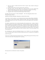
Settings > MQ Module Configuration:



‚System type‛ must be ‚Quantum‛
The ‚GPS‛ box must be checked.
All other boxes must be unchecked.
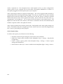
Settings > Advanced:





15
The unlock code must be entered.
You must contact MaxQData by email or phone and
provide the number in the grey box at the top of the screen (the ‚challenge code‛) in order to
receive your unlock code. If you do not enter this, you will have only 1 Hz sampling.
‚Racing type‛ should be set to the kind of racing you will be doing.
‚Log type 1 records only‛ must be unchecked.
‚Open before trigger‛ should be checked.
‚Debug mode‛ and ‚Log serial‛ should be unchecked.


‚MQ ticks/s‛ must be 1000.
The remaining settings may be left at their defaults values.
Step 3 – Module Configuration
There is a text file stored on the Quantum that contains important configuration information. This
text file must be changed to enable Standalone operation.
Plug the Quantum into the USB port of a Windows PC. The Quantum will install as a ‚removable
drive‛. Open this drive in File Explorer and look for the file ‚quantum_config.txt‛. Open this file in
Notepad by double-clicking on it. Read through the file and make the following changes:
‚EnableLogging,0‛ – change the 0 to a 1
‚EnableBluetooth,1‛ or ‚EnableWiFi,1‛ – change the 1 to a 0 (this disables wireless altogether; if you
still wish to use the wireless connection while logging to internal memory, do not change this setting)
Save the file and exit from Notepad. Please see the chapter titled ‚Quantum Configuration‛ for more
information regarding configuring the Quantum.
Step 3 - Mounting
Mount the Quantum where it can see as much of the sky as possible and is level. The best location is
on top of the car, on the roof, where nothing is blocking its view. Under the front or rear windshield
are also acceptable locations as long as your car does not have infrared-reflecting glass. Please note
that the Quantum itself is not waterproof.
Be sure that the Quantum is mounted in the correct orientation. The blue arrow should be pointing
forward. The USB port should be at the back.
On models that do not have a magnetic base, it is necessary to devise your own mounting method.
This can be as simple as duct tape.
On models with a magnetic base, please be aware that while the magnets are very strong, the module
could blow off the roof if you go fast enough, especially with severe headwinds or crosswinds.
MaxQData does not guarantee that the magnets will hold under all conditions. Some applications
will still require duct tape or fasteners to hold the unit in place.
Step 4 – Trial Run
After changing the settings in Step 2, the Quantum will be configured to log data once the vehicle
reaches 20 MPH (including approximately ten seconds’ worth of data before this point), and then
stop logging when the vehicle comes below 15 MPH for more than 5 seconds. So, for a trial run, all
you need to do after mounting the unit is turn the unit on, wait green light to begin flashing, wait
further until the green flash becomes short and quick, and then drive.
16
Step 5 – View Flight Recording on laptop/desktop
Turn off the Quantum. Connect it to your PC using the USB cable. Turn on the Quantum. The
Quantum will install as a Removable Drive. Open this drive and look for files named something like
‚Quantum 090201 1534.txt‛. There will be one file for each time the Flight Recording Trigger was
activated. Copy these files to your PC’s My Documents folder. Now run MaxQData Flight. When
Flight opens, it will ask you to select a file that you want to process. Find the first file you copied
from the Quantum, select it, and click OK. Flight will process the data and then exit. You should
now see a flight recording file in the My Documents folder with the name Run000.mqd. Double-click
on this file to open it. MaxQData Chart will launch and automatically load the file for analysis.
17
Quantum™ Quickstart Guide – Connected Operation – Bluetooth
Models
Thank you for purchasing a MaxQData™ MQGPS™ system. If you have any problems getting
started, you can send email to [email protected].
PLEASE NOTE – IF YOU PURCHASED YOUR QUANTUM AS PART OF A COMPLETE SYSTEM
FROM MAXQDATA, DO NOT FOLLOW THIS QUICKSTART GUIDE. THE SYSTEM IS ALREADY
SET UP FOR YOU.
‚Connected‛ operation means that the Quantum™ will capture data and immediately send it to a
Pocket PC or laptop via Bluetooth. This is also the normal configuration for a VeQtr™ system. If you
wish to use ‚Standalone‛ operation where the Quantum does not use Bluetooth and instead records
to internal memory, please refer to the Quantum Quickstart Guide for ‚Standalone Operation‛.
Battery Charging
The Quantum charges from any USB port. Use the included USB-to-mini USB cable for charging.
The status light will glow red while the battery is charging and will turn off when the battery is done
charging. Maximum charge time is typically 2-3 hours. The battery is internal and should last the life
of the system but can be replaced by the user if necessary – contact MaxQData for details. An
optional double capacity battery is available. Be sure to switch off the Quantum when not in use (run
time on a full charge is 8-10 hours).
Quantum Status Light




Red means charging
Flashing green means data is being received from the GPS satellites. This flash will turn into
a shorter, quicker flash once satellite lock is achieved.
Flashing blue means data is being transmitted over Bluetooth.
When the unit is turned on, the blue and green lights both turn on, then the blue light turns
off, and then the green light turns off. The green light will then begin flashing when GPS
data is received.
Step 1 – Software Download and Installation – Laptop/Desktop
Download the latest software from the MaxQData website. You will need the file labeled ‚PC
Complete System Software‛, not the one labeled ‚PC Chart Only‛. The name of the file will be
similar to ‚MaxQData 31a PC Software.exe‛. Download the file to your laptop and double-click on it
to run it. Do not install the ‚TraQr Manager‛ application. Also do not install any MQGPS drivers.
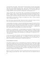
Step 2 - Bluetooth Pairing with a Windows Mobile 2003 Pocket PC
18











Turn on the MQGPS.
Tap the Bluetooth icon at the lower right of the Today screen and turn on Bluetooth.
Run the Bluetooth Manager from the Bluetooth icon.
Tap ‚New‛, and then ‚Explore a Bluetooth Device‛. The Pocket PC will search for new
Bluetooth devices. An icon should appear for the GPS module (common names are ‚iBT-GPS‛
(MQGPS-5Hz) or ‚G-Rays I‛ (MQGPS-HiDef)‛. There may also be a checkbox titled
‚Always use the selected device‛; be sure to check this checkbox. Then tap the icon for the
MQGPS.
Select ‚Serial Port‛ and ‚Next‛. A shortcut will be created.
Go back to the Today screen and select ‚Bluetooth Settings‛ from the Bluetooth icon.
Tap the ‚Services‛ tab.
Tap ‚Serial Port‛. Check ‚Enable service‛. Uncheck the other checkboxes.
Tap ‚Advanced‛ and make a note of the ‚Outbound COM Port‛.
Tap ‚OK‛ and ‚OK‛ again to get out of the Bluetooth Settings applet.
Note: if you are asked for a passkey for the Quantum, it is 1234.
Run MaxQData Setup and go to Settings > Serial Port Settings. For ‚GPS Port‛, enter ‚COMx‛,
where ‚x‛ is the number of the Outbound COM Port. Note: if the port is COM10 or higher, you will
need to enter it as \\.\COM10 . Select ‚Is Bluetooth‛ under ‚GPS Port‛.
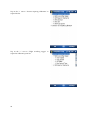
Step 2 – Bluetooth Pairing with certain Windows Mobile 5 and 6 Pocket PCs, such as the ASUS A626
and HP iPAQ series
A few Pocket PCs based on Windows Mobile 5 or 6 use the same pairing process as the one above for
Windows Mobile 2003 devices. However, the Bluetooth manager may not be available on the Today
screen. You can access the Bluetooth manager from Start > Settings > Connections > Bluetooth.
Step 2 – Bluetooth Pairing with other Windows Mobile 5 and 6 Pocket PCs – Dell Axim X51, etc.










19
Turn on the MQGPS.
Tap the Bluetooth icon at the lower right of the Today screen.
Check ‚Turn on Bluetooth‛. You can either check or uncheck ‚Make this device
discoverable‛.
Go to the ‚Devices‛ tab and tap ‚New Partnership...‛. The Pocket PC will scan for Bluetooth
devices. An entry for the GPS module (e.g. ‚iBT-GPS‛ (MQGPS-5Hz) or ‚G-Rays I‛
(MQGPS-HiDef)) will appear. Tap this entry and then ‚Next‛.
Enter ‚1234‛ for the passkey (no quotes) and tap ‚Next‛.
Check the ‚Serial Port‛ box and tap ‚Finish‛.
Go to the ‚COM Ports‛ tab.
Tap ‚New Outgoing Port‛
Select your Socket BT GPS module and tap ‚Next‛.
Choose a COM port to use for the connection. ‚COM7‛ is recommended if available.
Uncheck ‚Secure Connection‛. Tap ‚Finish‛. If an error is displayed indicating that the
COM port is not available, try another. Note: on a Pocket PC Phone Edition device, your
choice of COM port may interfere with the ‚Wireless Modem‛ function. If you find that you
are unable to use the PPCPE as a wireless data modem after pairing the MQGPS, delete the
Outgoing Port and try a different COM port number.
Run MaxQData Setup and go to Settings > Serial Port Settings. For ‚GPS Port‛, enter ‚COMx‛,
where ‚x‛ is the number of the Outbound COM Port. Note: if the port is COM10 or higher, you will
need to enter it as \\.\COM10 . Select ‚Is Bluetooth‛ under ‚GPS Port‛.
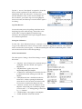
Step 2 – Bluetooth Pairing with a Windows XP notebook PC
Please note that there are many different Bluetooth vendors and they all too often use their own
software instead of the Bluetooth software that is built in to Windows XP SP2, which can make it
difficult for users to set up Bluetooth because of a lack of standard procedure. Here we provide
instructions based on the standard Windows XP Bluetooth software. If your Bluetooth software
is different, you will need to figure out how to do the same procedure. Consult your Bluetooth
user’s guide or online sources for assistance.






Turn on the Quantum.
Click Start > Control Panel, then double-click Bluetooth Devices.
On the Devices tab, click Add... to get the ‚Add Bluetooth Device Wizard‛. Proceed through
the wizard and allow the wizard to search for nearby devices. The icon for the Quantum
should appear. If it doesn’t, click Search Again. Click Next.
Enter 1234 for the security code and click Pair Now.
On the next screen, check the ‚Serial Port Service‛ checkbox, click Configure, write down the
COM port number, uncheck ‚Secure Connection‛, and click OK.
Finish out the wizard.
Run MaxQData Setup and go to Settings > Serial Port Settings. For ‚GPS Port‛, enter ‚COMx‛,
where ‚x‛ is the number of the Outbound COM Port. Note: if the port is COM10 or higher, you will
need to enter it as \\.\COM10 . Select ‚Is Bluetooth‛ under ‚GPS Port‛.
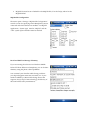
Step 3 – Software Setup for Connected Operation
Run MaxQData Setup and configure the software according to the following settings:
Settings > Serial Port Settings:









20
‚MQ Port‛ must be ‚NONE‛ (all caps, no quotes).
‚Is Bluetooth‛ under ‚MQ Port‛ does not matter.
‚MQ Baud Rate‛ does not matter
‚Delay Bluetooth Init‛ should be checked on a Pocket PC, unchecked on a notebook PC.
‚GPS Port‛ must be the COM port assigned earlier during Bluetooth pairing.
‚Is Bluetooth‛ under ‚GPS Port‛ should be checked.
‚GPS Baud Rate‛ does not matter.
‚Enable $GPRGH‛ must be checked.
‚GPS Hz‛ should be set to ‚Default‛.
Settings > MQ Module Configuration:



‚System type‛ must be ‚Quantum‛
The ‚GPS‛ box must be checked.
All other boxes must be unchecked.
Settings > Advanced:







The unlock code must be entered.
You must contact MaxQData by email or phone and
provide the number in the grey box at the top of the screen (the ‚challenge code‛) in order to
receive your unlock code. If you do not enter this, you will have only 1 Hz sampling.
‚Racing type‛ should be set to the kind of racing you will be doing.
‚Log type 1 records only‛ must be unchecked.
‚Open before trigger‛ should be checked.
‚Debug mode‛ and ‚Log serial‛ should be unchecked.
‚MQ ticks/s‛ must be 1000.
The remaining settings may be left at their defaults values.
Step 4 – Verify the Connection
Exit from MaxQData Setup (on a Pocket PC, use File > Exit, do not use the ‚X‛ button). Place the
Quantum where it has good visibility of the sky and turn it on. Wait for GPS lock (fast, short green
blinks). Run MaxQData Flight. If this is the first time you have run the software, it will read ‚No
sensors configured‛. Go into Configure > Sensors, select ‚Standard‛, then click ‚OK‛. You may be
prompted to select a Bluetooth device. If present, check the ‚Always use the selected device‛
checkbox if it appears. Next, tap the icon for the Quantum. After a short wait, the connection to the
Quantum will be established and you should see a satellite count greater than zero appear on the
screen. The system is now ready to use.
Note: If the Quantum has been turned off for a long time, or if it has been shipped across country, it
may take several minutes to achieve satellite lock (12.5 minutes worst case, but normally under 5
minutes).
Step 5 - Mounting
Mount the Quantum where it can see as much of the sky as possible and is level. The best location is
on top of the car, on the roof, where nothing is blocking its view. Under the front or rear windshield
are also acceptable locations as long as your car does not have infrared-reflecting glass. Please note
that the Quantum is not waterproof.
Be sure that the Quantum is mounted in the correct orientation. The blue arrow should be pointing
forward. The USB port should be at the back.
21
If you are using a Pocket PC, you can mount it to the dashboard or place it in a storage compartment.
Be sure that nothing can accidentally tap the screen.
If you are using a notebook PC, you may be able to mount it by simply squeezing it between the seat
cushion and the center console, or place it in a map pocket.
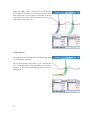
Step 6 – Trial Run
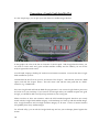
With the Quantum turned on and the Pocket PC or laptop running Flight, do a test run. Be sure to
reach a speed above 20 MPH in order to trigger a flight recording. After your run, come to a stop,
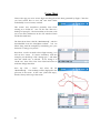
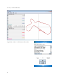
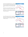
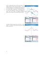
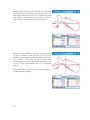
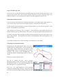
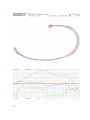
then run MaxQData Chart and load the file you just created, which should be named ‚Run000‛. Tap
Map > Full GPS Map‛ if necessary to see your complete GPS trackmap. Your car is at the ‚+‛ sign.
Tap one of the fields which reads ‚Select...‛ and choose ‚GPS Vehicle speed‛. This will bring up a
vehicle speed data trace on the screen in the crosshair plot area. To move the data forward in time,
tap and drag the plot area to the left. As you move the data forward in time, you will see the ‚+‛ sign
move around the trackmap.
22
Quantum™ and Quantum Dot™ Quickstart Guide – Connected
Operation – WiFi Models
Thank you for purchasing a MaxQData™ Quantum™ system. If you have any problems getting
started, you can send email to [email protected].
PLEASE NOTE – IF YOU PURCHASED YOUR QUANTUM AS PART OF A COMPLETE SYSTEM
FROM MAXQDATA, DO NOT FOLLOW THIS QUICKSTART GUIDE. THE SYSTEM IS ALREADY
SET UP FOR YOU.
‚Connected‛ operation means that the Quantum™ will capture data and immediately send it to a
Pocket PC or laptop via Bluetooth. This is also the normal configuration for a VeQtr™ system. If you
wish to use ‚Standalone‛ operation where the Quantum does not use Bluetooth and instead records
to internal memory, please refer to the Quantum Quickstart Guide for ‚Standalone Operation‛.
Batteries – Models that use AA batteries
Run time with rechargeable NiMH batteries is about 5 hours. Alkaline batteries should last about
half this time. Disposable lithium batteries should last about double. Be sure to switch off the
Quantum when not in use. For endurance racing or other applications requiring continuous power,
you can omit the batteries and connect a 2.5V-3.0V, 500 mA, regulated and filtered power supply.
Status Lights – Models that use AA batteries







Red slow flash: power is on
Red fast flash: low battery
Solid red: Standby
Green slow flash: GPS searching, unit not ready for use
Green fast flash: GPS locked, unit is ready for use
Blue slow flash: Wireless is connected
Blue fast flash: Transmitting data
Step 1 – Software Download and Installation – Laptop/Desktop
Download the latest software from the MaxQData website. You will need the file labeled ‚PC
Complete System Software‛, not the one labeled ‚PC Chart Only‛. The name of the file will be
similar to ‚MaxQData 31a PC Software.exe‛. Download the file to your laptop and double-click on it
to run it. Do not install the ‚TraQr Manager‛ application. Also do not install any MQGPS drivers.
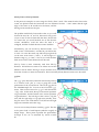
Step 2 – WiFi Setup for Netbooks
1.
Make sure the Quantum is turned on and locked to the satellites (fast flashing green light).
This can take 5-10 minutes the first time it is turned on after installing batteries. You may
23
need to power cycle the Quantum if it goes into standby (solid red light). We recommend
going outside for a clear view of the sky.
2.
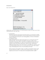
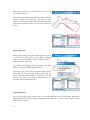
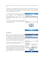
Start > Control Panel > Network Connections. Double-click the Wireless Network
Connection to bring up the ‚Choose a wireless network‛ wizard. Look for the SSID of the
WiFi Quantum in this list (it will be something like ‚MaxQDataQTM090820A‛). Click
‚Refresh network list‛ if it does not appear. Click on the list entry for the Quantum to select
it, then click the Connect button. Once connected, click ‚Change advanced settings‛. Scroll
through the list to find ‚Internet Protocol (TCP/IP)‛. Click on it to select, then click
‚Properties‛. Select ‚Use the following IP address‛. IP address should be 169.254.1.2, and
subnet mask should be 255.255.0.0. All other fields should be blank. Click OK. Click on the
Wireless Networks tab. In the ‚Preferred networks‛ box, select the entry for the Quantum,
then click ‚Properties‛. Click the ‚Connection‛ tab, then check the checkbox labeled
‚Connect when this network is in range‛. Click OK, then click OK.
3.
Run MaxQData Settings. Settings > Serial Port Settings ‚GPS Port‛ : type in 169.254.1.1:2000
(no spaces). Leave the remaining settings at their defaults and close this window. Go to
Settings > MQ Module Configuration. If your module is a Quantum, set System Type to
Quantum, but if your module is a Quantum Dot, set System Type to MQGPS. Make sure the
GPS box is checked, then close this window. Go to Settings > Advanced. Enter the unlock
response code under Advanced Settings (send MaxQData the challenge code in the grey box
in order to receive the response code). Set Racing Type to the type of racing you expect to do.
Leave the remaining settings at their defaults and close this window.
Step 4 – Verify the Connection
Exit from MaxQData Setup. Place the Quantum where it has good visibility of the sky and turn it on.
Wait for GPS lock (fast, short green blinks). Run MaxQData Flight. If this is the first time you have
run the software, it will read ‚No sensors configured‛. Go into Configure > Sensors, select
‚Standard‛, then click ‚OK‛. After a short wait, the connection to the Quantum will be established
and you should see a satellite count greater than zero appear on the screen. The system is now ready
to use.
Note: If the Quantum has been turned off for a long time, or if it has been shipped across country, it
may take several minutes to achieve satellite lock (12.5 minutes worst case, but normally under 5
minutes). Also, if the unit sees less than half the sky, initial lock may take a very long time.
Step 5 - Mounting
Mount the Quantum where it can see as much of the sky as possible. The best location is on top of
the car, on the roof, where nothing is blocking its view. Under the front or rear windshield are also
acceptable locations as long as your car does not have infrared-reflecting glass. Please note that the
Quantum and Quantum Dot are not waterproof.
24
If you have a Quantum Dot, the mounting orientation is not critical as long as the top of the module
is facing the sky.
If you have a Quantum, be sure that the Quantum is mounted in the correct orientation. The blue
arrow must be pointing forward. The top of the module must face the sky. The module must be
level.
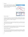
Step 6 – Trial Run
With the Quantum turned on and the Pocket PC or laptop running Flight, do a test run. Be sure to
reach a speed above 20 MPH in order to trigger a flight recording. After your run, come to a stop,
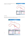
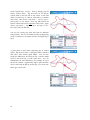
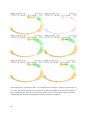
then run MaxQData Chart and load the file you just created, which should be named ‚Run000‛. Tap
Map > Full GPS Map‛ if necessary to see your complete GPS trackmap. Your car is at the ‚+‛ sign.
Tap one of the fields which reads ‚Select...‛ and choose ‚GPS Vehicle speed‛. This will bring up a
vehicle speed data trace on the screen in the crosshair plot area. To move the data forward in time,
tap and drag the plot area to the left. As you move the data forward in time, you will see the ‚+‛ sign
move around the trackmap.
25
MQGPS-5Hz™ and MQGPS-HiDef™ Quickstart Guide
Thank you for purchasing a MaxQData™ MQGPS™ system. If you have any problems getting
started, you can send email to [email protected].
PLEASE NOTE – IF YOU PURCHASED YOUR MQGPS AS PART OF A COMPLETE SYSTEM FROM
MAXQDATA, DO NOT FOLLOW THIS QUICKSTART GUIDE. THE SYSTEM IS ALREADY SET UP
FOR YOU.
This quickstart guide assumes you are using an MQGPS-5Hz or MQGPS-HiDef with a Pocket PC.
TraQr and Quantum users should refer to the respective Quickstart Guides.
Battery Installation and Charging
Install the battery into the MQGPS. All MQGPS models have a standard 5V Mini-USB charging port.
This allows you to use the charger that comes with the MQGPS, or a USB sync cable, or a Pocket PC
charger. Maximum charging time is about three hours. Charging status is indicated by the LED
Power Status Indicator.
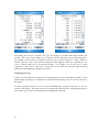
MQGPS-5Hz LED Status Indicators
LED Power Status Indicator (Red/Green):
 Solid Red: battery power is low, needs recharging
 Solid Green: battery is charging
 Blinking Green: battery is fully charged
LED Bluetooth status indicator (Blue):
 Solid Blue: Bluetooth not connected, or pairing initiated
 Flashes once per second: Bluetooth is connected
 Flashes once every five seconds: Standby mode
LED GPS Status Indicator (Orange):
 Solid Orange: no satellite lock, searching for satellites
 Flashing: satellites locked
MQGPS-HiDef LED Status Indicators
LED Power/GPS Status Indicator (Red + Green):
There are two LEDs in this indicator: Red and Green. Together, they make Orange. The Red LED
blinks when the battery is low. On charge, the Red LED is solid on. When fully charged, the Red
LED turns off. The Green LED is on when the unit is powered on. It blinks once per second when
the unit has satellite lock, otherwise it is solid on.
LED Bluetooth status indicator (Blue):
 Solid Blue: Bluetooth not connected
 Flashes once per second: Bluetooth is connected
 Flashes once every five seconds: Standby mode
NOTE: The ‚X‛ in the upper right corner of the Pocket PC screen does not close an application. It
minimizes it. Always use File > Exit to truly exit from any MaxQData application.
26
IF YOU ORDERED YOUR MQGPS WITH A POCKET PC, YOU DO NOT NEED TO PAIR IT. ALL
SOFTWARE HAS BEEN LOADED AND CONFIGURED FOR YOU. TO OPERATE:
Turn on the MQGPS. Wait for satellite lock (see status indicator description above). Be sure the
MQGPS is in a window or outside and has a good view of at least 50% of the sky. If the MQGPS does
not lock to the satellites before going into power saving mode, proceed to step B) anyways.
Find the ‚record‛ button on your Pocket PC. On the ASUS A626, this is the button on the front of the
device with the ‚microphone‛ icon. Press this button. The Pocket PC will turn on and Flight will run
automatically. You will see the blue LED on the MQGPS begin to blink. After a short wait, you
should see live data on the screen. If your MQGPS was just shipped a long distance, it might take a
few minutes for live data to show, up to 15 minutes worst case. Be sure to place the MQGPS outside
for quickest satellite lock.
Position the MQGPS securely in the car or on the roof so it can see as much of the sky as possible for
maximum accuracy.
Drive. Data will be collected automatically as long as the car exceeds 20 MPH.
IF YOU PURCHASE THE MQGPS BY ITSELF, YOU WILL NEED TO PAIR IT WITH YOUR POCKET
PC AND SET UP THE SOFTWARE ACCORDING TO THE INSTRUCTIONS BELOW.
Step 1 - Partnering your Pocket PC with Windows 2000 or Windows XP
Before you can connect your Pocket PC to your laptop or desktop PC, you must first download and
install the ‚ActiveSync‛ application from Microsoft. You may also have ActiveSync on the CD-ROM
that came with your Pocket PC, but it is recommended to download the latest version from the
Microsoft website. You can find this quickly by going to www.microsoft.com and searching for
‚ActiveSync‛. Install ActiveSync, then follow the on-screen instructions for connecting to and setting
up a partnership with your Pocket PC. From then on, ActiveSync will run automatically when you
connect your Pocket PC.
You can transfer files by clicking the ‚Explore‛ button in the ActiveSync window. The initial file
explorer window shows the ‚\My Documents‛ folder on the Pocket PC, which is where you will find
all your data files unless you change the location later.
Step 1 - Partnering your Pocket PC with Windows Vista
Setting up a Pocket PC is automatic under Windows Vista. Do not install ActiveSync. Instead, you
need to use ‚Windows Mobile Device Center‛. First, be sure that your PC is connected to the Internet.
Then connect your Pocket PC to your PC using the USB cable that came with it. Windows Vista will
recognize the device and automatically download and install Windows Mobile Device Center from
Microsoft. Follow the on-screen instructions for setting up a partnership with your Pocket PC. From
then on, Windows Mobile Device Center will run automatically when you connect your Pocket PC.
You can also access it from the Control Panel.
27
You can transfer files by clicking ‚Browse the contents of your device‛ under ‚File Management‛.
The initial file explorer window shows the root folder ‚\‛ and may also show a Storage Card folder.
Double-click on ‚\‛, then double click on ‚\My Documents‛. This is the folder where you will find
all your data files unless you change the location later.
Step 2 - Software Download and Installation – Pocket PC
Download the latest software from the MaxQData website. You will need the file labeled as the
‚Pocket PC Complete System Software‛. The name of the file will be similar to ‚MaxQData 31a PPC
Software.exe‛. Transfer this file to the \My Documents folder on your Pocket PC using ActiveSync
or Windows Mobile Device Center as explained above. Then on the Pocket PC, tap Start > Programs >
File Explorer (it may also be found on the Start menu). You should see the \My Documents folder; if
not, navigate to that folder. Locate the installation file and tap its name to install the MaxQData
software. This will install the Chart, Flight, and Setup applications. Chart is for data analysis, Flight
is for collecting the data, and Setup is for setup and calibration. After installing the software, delete
the install file from the Pocket PC.
Step 3 – Software Download and Installation – Laptop/Desktop
Again, download the latest software from the MaxQData website. You will need the file labeled as
‚PC Chart Only‛. The name of the file will be similar to ‚MaxQData 31a PC Chart.exe‛. Download
the file to your laptop and double-click on it to run it. This will install only the Chart software on
your PC, which is what you will need to do data analysis.
Step 4 - Pairing with a Windows Mobile 2003 Pocket PC




Turn on the MQGPS.
Tap the Bluetooth icon at the lower right of the Today screen and turn on Bluetooth.
Run the Bluetooth Manager from the Bluetooth icon.
Tap ‚New‛, and then ‚Explore a Bluetooth Device‛. The Pocket PC will search for new
Bluetooth devices. An icon should appear for the GPS module (common names are ‚iBT-GPS‛
(MQGPS-5Hz) or ‚G-Rays I‛ (MQGPS-HiDef)‛. There may also be a checkbox titled
‚Always use the selected device‛; be sure to check this checkbox. Then tap the icon for the
MQGPS.
 Select ‚Serial Port‛ and ‚Next‛. A shortcut will be created.
 Go back to the Today screen and select ‚Bluetooth Settings‛ from the Bluetooth icon.
 Tap the ‚Services‛ tab.
 Tap ‚Serial Port‛. Check ‚Enable service‛. Uncheck the other checkboxes.
 Tap ‚Advanced‛ and make a note of the ‚Outbound COM Port‛.
 Tap ‚OK‛ and ‚OK‛ again to get out of the Bluetooth Settings applet.
 Run MaxQData Setup and go to Settings > Serial Port Settings. For ‚GPS Port‛, enter
‚COMx‛, where ‚x‛ is the number of the Outbound COM Port. Select ‚Is Bluetooth‛ under
‚GPS Port‛. Continue with the remaining setup as described below under ‚MQGPS Setup‛.
If you are ever asked for a passkey for the MQGPS-5Hz or MQGPS-HiDef, it is ‚0000‛ (no quotes).
28
Step 4 - Pairing with certain Windows Mobile 5 and 6 Pocket PCs, such as the ASUS A626 and HP
iPAQ series
A few Pocket PCs based on Windows Mobile 5 or 6 use the same pairing process as the one above for
Windows Mobile 2003 devices. However, the Bluetooth manager may not be available on the Today
screen. You can access the Bluetooth manager from Start > Settings > Connections > Bluetooth.
Step 4 - Pairing with other Windows Mobile 5 Pocket PCs – Dell Axim X51, etc.











Turn on the MQGPS.
Tap the Bluetooth icon at the lower right of the Today screen.
Check ‚Turn on Bluetooth‛. You can either check or uncheck ‚Make this device
discoverable‛.
Go to the ‚Devices‛ tab and tap ‚New Partnership...‛. The Pocket PC will scan for Bluetooth
devices. An entry for the GPS module (e.g. ‚iBT-GPS‛ (MQGPS-5Hz) or ‚G-Rays I‛
(MQGPS-HiDef)) will appear. Tap this entry and then ‚Next‛.
Enter ‚0000‛ for the passkey (no quotes) and tap ‚Next‛.
Check the ‚Serial Port‛ box and tap ‚Finish‛.
Go to the ‚COM Ports‛ tab.
Tap ‚New Outgoing Port‛
Select your Socket BT GPS module and tap ‚Next‛.
Choose a COM port to use for the connection. ‚COM7‛ is recommended if available.
Uncheck ‚Secure Connection‛. Tap ‚Finish‛. If an error is displayed indicating that the
COM port is not available, try another. Note: on a Pocket PC Phone Edition device, your
choice of COM port may interfere with the ‚Wireless Modem‛ function. If you find that you
are unable to use the PPCPE as a wireless data modem after pairing the MQGPS, delete the
Outgoing Port and try a different COM port number.
Run MaxQData Setup and go to Settings > Serial Port Settings. For ‚GPS Port‛, enter
‚COMx‛, where ‚x‛ is the number of the Outbound COM Port. Select ‚Is Bluetooth‛ under
‚GPS Port‛.
Step 5 - Setup
After installing the software and pairing the MQGPS with your Pocket PC, run MaxQData Setup and
check the following settings.
Settings > Serial Port Settings:
 ‚MQ Port‛ must be ‚NONE‛ (all caps).
 ‚Is Bluetooth‛ under ‚MQ Port‛ may be either checked or unchecked.
 ‚MQ Baud Rate‛ does not matter
 ‚Delay Bluetooth Init‛ should be checked.
 ‚GPS Port‛ must be set to the outgoing COM port you established earlier. NOTE: If the
COM port is numbered COM10 or higher, you must enter it using this notation: \\.\COM10 .
 ‚GPS Baud Rate‛ should be ‚38400‛.
 ‚Enable $GPRGH‛ must be checked.
29






‚Is Bluetooth‛ under ‚GPS Port‛ should be checked.
‚GPS Hz‛ must be ‚Default‛ for the MQGPS-5Hz, or ‚10‛ for the MQGPS-HiDef.
Settings > MQ Module Configuration:
‚System type‛ must be ‚MQGPS‛
The ‚GPS‛ box must be checked.
All other boxes must be unchecked.
Settings > Advanced:
The unlock code must be entered. Different Pocket PCs will require different unlock codes. You must
contact MaxQData by email or phone and provide the number in the grey box at the top of the screen
(the ‚challenge code‛) in order to receive your unlock code. If you do not enter this, you will have
only 1 Hz sampling.
 ‚Racing type‛ should be set to the kind of racing you expect to be doing most often.
 ‚Log type 1 records only‛ must be unchecked.
 ‚Open before trigger‛ should be checked (but see the manual for details on how to use this
option when hot-swapping data cards during pit stops).
 ‚Debug mode‛ and ‚Log serial‛ should be unchecked.
 ‚MQ ticks/s‛ must be 1000.
 The remaining settings may be left at their defaults values.
Step 6 – Verify the Connection
Exit from MaxQData Setup (use File > Exit, do not use the ‚X‛ button). Place the MQGPS where it
has good visibility of the sky and turn it on. Wait for the GPS LED indicator to go from solid
(searching) to blinking (locked). Run MaxQData Flight. If this is the first time you have run the
software, it will read ‚No sensors configured‛. Go into Configure > Sensors, select ‚Standard‛, then
click ‚OK‛. You may be prompted to select a Bluetooth device. If present, check the ‚Always use the
selected device‛ checkbox if it appears. Next, tap the icon for the MQGPS. After a short wait, the
connection to the MQGPS will be established and you should see a satellite count greater than zero
appear on the screen. The system is now ready to use.
Note: If the unit has been turned off for a long time, or if it has been shipped across country, it may
take several minutes to achieve satellite lock (12.5 minutes worst case, but normally under 5 minutes).
Step 7 - Mounting
Mount the MQGPS where it can see as much of the sky as possible and is approximately parallel to
the ground. The best location is on top of the car, on the roof, where nothing is blocking its view.
Under the front or rear windshield are also acceptable locations as long as your car does not have
infrared-reflecting glass. Still, these locations are not as good as a roof mount because the roof will
block a big chunk of the sky. MaxQData has magnetic roof mount covers for the MQGPS systems.
The Pocket PC can be mounted where the driver will see it, for example by velcroing it to the
dashboard, or it can be stowed in a glove box as long as the screen lock or screen cover is on. If you
expect wet conditions, put the MQGPS and the Pocket PC in a watertight bag or plastic box.
30
Step 8 – Trial Run
With the MQGPS turned on and the Pocket PC running Flight, do a test run. Be sure to reach a speed
above 20 MPH in order to trigger a flight recording. After your run, come to a stop, then run
MaxQData Chart and load the file you just created, which should be named ‚Run000‛. Tap Map >
Full GPS Map‛ if necessary to see your complete GPS trackmap. Your car is at the ‚+‛ sign. Tap one
of the fields which reads ‚Select...‛ and choose ‚GPS Vehicle speed‛. This will bring up a vehicle
speed data trace on the screen in the crosshair plot area. To move the data forward in time, tap and
drag the plot area to the left. As you move the data forward in time, you will see the ‚+‛ sign move
around the trackmap.
Step 9 – View Flight Recording on PC
Reconnect your Pocket PC to your PC. Using ActiveSync or Windows Mobile Device Center, open
the \My Documents folder on the Pocket PC. You should see the ‚Run000.mqd‛ flight recording file.
Drag and drop this file to your desktop, then double-click on it. MaxQData Chart will launch and
automatically load the file. Be sure to select the correct racing type under ‚File > Racing type...‛. You
may need to exit and restart Chart for this to take effect.
31
TraQr™ Quickstart Guide
Thank you for purchasing a MaxQData™ MQGPS™ system. If you have any problems getting
started, you can send email to [email protected].
Mode Switch
The power switch on the side of the unit has three positions: OFF, NAV, and LOG. OFF turns the
unit off. NAV enables NMEA data output via Bluetooth or USB for use by third party navigation
software or by MaxQData Flight. LOG enables on the built-in logging function. Please note that
when in NAV mode, the unit will go into standby when there is no Bluetooth connection, but in LOG
mode the unit does not go into standby.
Battery Installation and Charging
Install the battery into the TraQr. All MQGPS models have a standard 5V Mini-USB charging port.
This allows you to use the charger that comes with the MQGPS, or a USB sync cable, or a Pocket PC
charger. Maximum charging time is about three hours. Charging status is indicated by the LED
Power Status Indicator.
TraQr LED Status Indicators
LED Power Status Indicator (Red/Green):
 Solid Red: battery power is low, needs recharging
 Solid Green: battery is charging
 Blinking Green: battery is fully charged
LED Bluetooth status indicator (Blue):
 Solid Blue: Bluetooth not connected, or pairing initiated
 Flashes once per second: Bluetooth is connected
 Flashes once every five seconds: Standby mode
 Blue LED will be off in LOG mode unless there is an active Bluetooth connection.
LED GPS Status Indicator (Orange):
 Solid Orange: no satellite lock, searching for satellites
 Flashing: satellites locked
Step 1 – Software Download and Installation – Laptop/Desktop
Download the latest software from the MaxQData website. You will need the file labeled as ‚PC
Complete System Software‛, not the one labeled ‚PC Chart Only‛. The name of the file will be
similar to ‚MaxQData 31a PC Software.exe‛. Download the file to your laptop and double-click on it
to run it. When prompted, be sure to install the ‚TraQr Manager‛ application.
32
Next, download and install the USB driver software for the TraQr from the MaxQData website. Once
the driver is installed, connect the TraQr to your PC and wait for the USB installation to complete.
Then, go into the Device Manager (under Windows XP, this is Start > Settings > Control Panel >
System > Hardware > Device Manager; under Windows Vista, this is Start > Control Panel > Device
Manager). Expand ‚Ports (COM & LPT)‛ and look for ‚CP210x USB to UART Bridge Controller
(COM21)‛. The COM port name in parentheses, COM21 in this case, is the COM port used by the
TraQr. Write it down for use in Step 2.
NOTE: If you do not see an entry under ‚Ports (COM & LPT)‛, then it is likely that you either have
not installed the drivers properly or they may need to be reinstalled. Unplug and replug the TraQr
while watching the Device Manager list. You should see it come up under ‚Other‛. The device will
be shown with a question mark over the icon. Right click on the icon and select ‚Reinstall driver‛.
You can also use a Pocket PC to download the data from the TraQr and review it. Simply install the
‚Pocket PC Complete System Software‛ onto your Pocket PC. The only way to extract data from the
TraQr using a Pocket PC is via Bluetooth. You will therefore need to pair the unit with your Pocket
PC. See the MQGPS Quickstart guide for pairing details.
Step 2 – Software Setup
Run MaxQData Setup and configure the software according to the following settings:
Settings > Serial Port Settings:









‚MQ Port‛ must be ‚NONE‛ (all caps).
‚Is Bluetooth‛ under ‚MQ Port‛ may be either checked or unchecked.
‚MQ Baud Rate‛ does not matter
‚Delay Bluetooth Init‛ should be unchecked.
‚GPS Port‛ must be set to the COM port you wrote down from Step 1. Please note: if your
COM port is COM10 or above, you must enter it as (for example) \\.\COM10 .
‚Is Bluetooth‛ under ‚GPS Port‛ should be unchecked.
‚GPS Baud Rate‛ must be ‚115200‛.
‚Enable $GPRGH‛ must be checked.
‚GPS Hz‛ must be ‚5‛.
Settings > MQ Module Configuration:



‚System type‛ must be ‚MQGPS‛
The ‚GPS‛ box must be checked.
All other boxes must be unchecked.
Settings > Advanced:

33
The unlock code must be entered.
You must contact MaxQData by email or phone and
provide the number in the grey box at the top of the screen (the ‚challenge code‛) in order to
receive your unlock code. If you do not enter this, you will have only 1 Hz sampling.






‚Racing type‛ should be set to the kind of racing you expect to be doing most often.
‚Log type 1 records only‛ must be unchecked.
‚Open before trigger‛ should be checked.
‚Debug mode‛ and ‚Log serial‛ should be unchecked.
‚MQ ticks/s‛ must be 1000.
The remaining settings may be left at their defaults values.
Step 3 - Mounting
Mount the MQGPS where it can see as much of the sky as possible and is approximately parallel to
the ground. The best location is on top of the car, on the roof, where nothing is blocking its view.
Under the front or rear windshield are also acceptable locations as long as your car does not have
infrared-reflecting glass. Still, these locations are not as good as a roof mount because the roof will
block a big chunk of the sky. MaxQData has a magnetic roof mount cover available for the TraQr.
Step 4 – Trial Run
The TraQr comes preconfigured to log data at 5 Hz when vehicle speed is above 20 MPH. So, for a
trial run, all you need to do after mounting the unit is flip the switch to ‚LOG‛, wait for the orange
light to flash indicating satellite lock, and then drive.
Step 5 – View Flight Recording on laptop/desktop
Be sure the power switch is in the LOG position. Connect the TraQr to your PC using the USB cable.
Run the MaxQData TraQr Manager application. Click the ‚Download‛ button. The software will
extract the data from the TraQr. You will see MaxQData Flight run automatically to process the data.
Wait for the download process to complete, including the erase and configure step. You should now
see flight recording file(s) in the Save As location (default is to save to your Documents folder using
the name RunXXX.mqd). Double-click on one of the flight recording files. MaxQData Chart will
launch and automatically load the file for analysis.
34
Mounting Considerations
MQGPS
To maintain accuracy, customers report that the best location for mounting the MQGPS is externally,
on the roof of the car. Although an interior mount, such as under the front windshield, can work well,
there are a few drawbacks:


The roof still blocks a big chunk of the sky, which means fewer satellites visible on average,
which means lower accuracy.
Some cars have an ‚athermic‛ infrared-reflecting window glass, or a heated windshield.
These windows have a thin, conductive coating on the glass which dramatically reduces GPS
signal strength.
If your car does not have a metal roof, then an inside mount should work about as well as an external
mount. Just don’t mount it down deep in a console box, where visibility to the horizon is blocked.
Your MQGPS-5Hz, TraQr, Quantum, or Quantum Dot is not waterproof. You can seal it up with
duct tape or put it in a plastic bag if necessary.
It is important to mount the MQGPS more or less level. There are no inertial accelerometers inside
the MQGPS that would be affected, but the GPS antenna needs to be approximately level with the
ground for best reception. +-20 degrees from level is a good rule of thumb, except for the Quantum.
With the Quantum, the best accuracy will be achieved with the accelerometers as close to level as
possible. If you are mounting the unit on the roof of the car, pick a location where the roof itself is
parallel to the ground (nearly all cars have a level spot between where the roof slopes down to meet
the front windshield and where it slopes back towards the rear) Run Flight and watch ‚GPS LatG‛
and ‚GPS LongG‛. These values should be near zero, though in practice they can be off zero by
several hundredths of a g without causing any real problems. It is often sufficient just to eyeball the
installation. But you can shim the module if necessary to zero these values.
Pocket PC/iPhone
There are numerous mounting solutions available for mounting Pocket PCs in cars. Check with a
vendor such as www.mobileplanet.com or www.ram-mount.com to see if there is anything that suits
your needs.
At MaxQData, our favorite approach is to fasten the Pocket PC to the dashboard with Velcro™. A
few judiciously applied strips on the back of the device and on the dashboard are usually enough to
hold under hard driving. Be careful when removing the Pocket PC so as not to pop off the battery
door on the back of the Pocket PC.
If you have Flight set up to trigger a flight recording automatically, then you can put the Pocket PC in
a glove box, center console, or otherwise hidden out of sight. Be sure to flip the screen lock switch or
close the screen cover to prevent the screen from being touched while operating.
35
Protect your Pocket PC from water, heat sources, and dirt. Use a protective case where necessary.
Laptop
If you are using a laptop for data collection, it will require a secure mounting solution. For
temporary use, it may be sufficient to store it in a map pocket. Other applications may require the
installation of a permanent hardmount. Keep in mind that the hard drives in laptops may become
damaged from excessive shock and vibration and cushion the laptop appropriately. Solid-state
drives (‚SSDs‛) are recommended for vehicles with extremely stiff suspensions. Companies like
www.ram-mount.com provide vehicle mounting solutions for laptops. If you are using a laptop to
perform video capture, be sure the laptop has plenty of ventilation because the intensive CPU usage
will raise the internal laptop temperature significantly.
36
Using the Quantum – Standalone Operation
The Quantum may be used as standalone GPS data acquisition module. When properly configured,
it’s extremely simple to use – just turn it on and drive. There is enough memory for over 120 hours of
continuous datalogging.
Since you do not need to use a Pocket PC with the Quantum, you do not need to learn much about
using the Flight application. Flight is only used to process the downloaded data in order to create a
flight recording file with the extension ‚MQD‛. Once the data is processed, you load the MQD file
into the Chart application to view it and add video.
Of course, when operating the Quantum in standalone mode, you will not have certain real-time
features, such as a dashboard lap timing display, although you will certainly be able to get lap and
segment times after you download the data.
Method of Operation
Here’s the basic process for using the Quantum:
1.
2.
3.
4.
5.
6.
Turn on the Quantum.
Wait for satellite lock. Watch the status light carefully to see how it changes. First, both the
blue and green lights turn on. Then the blue light turns off, and then the green light. Then
the green light will begin flashing at a steady pace. This indicates that the module is
receiving GPS data but has not locked to the satellites yet. Once satellite lock is achieved, the
green light flashes faster, with shorter flashes.
Drive. Data will be collected automatically when the car reaches 20 MPH (depending on the
setting of the flight recording trigger).
Download the data to a laptop. This is quite simple since the Quantum acts like a USB
memory stick.
Process the data with Flight. This generates the .MQD flight recording files used by Chart.
View the data in Chart.
Setup
Please follow the Quantum Quickstart Guide earlier in this manual to ensure proper setup. Be sure
to set the ‚GPS Port‛ setting in MaxQData setup to ‚TXT‛.
Attaching the Quantum to a PC
The Quantum emulates a USB memory stick, making it very easy to move data off of it to a PC. You
must turn off the Quantum before you connect it to the PC. If the Quantum is turned on and it does
not have a USB connection, it goes into data capture mode and stays there until it is turned off.
The Quantum appears as a removable drive. You use the Windows File Explorer to open up the
drive and browse the files.
37
Files Created on the Quantum
The Quantum stores the captured data in files with special names based on the date and time, e.g.
‚Quantum 090201 1621.txt‛ means that the file was created on February 1, 2009 at 4:21 PM. These
files are simple text files that contain the NMEA data from the GPS calculations. It is necessary to run
each file through Flight in order to create a usable flight recording file. Flight recording files are
named with the extension ‚.MQD‛.
Be sure to occasionally delete any files you no longer need.
Running Flight
Because you configured the ‚GPS Port‛ setting in MaxQData Setup to be ‚TXT‛ and not a COM port,
Flight understands that it is operating in Standalone mode. In this mode, when you start Flight,
instead of attempting to connect to the Quantum over Bluetooth, it presents a file explorer window
that allows you to select one of the files captured by the Quantum. Once you have done this, Flight
will process the data in that file to create the MQD flight recording file. These files will be placed in
your My Documents folder and will be named ‚RunXXX.MQD‛ where ‚XXX‛ is a sequence number.
Flight enables the following sensors in this mode:














Flight recording trigger
GPS Altitude
GPS Latitude
GPS Longitude
GPS Satellite count
GPS HDOP
GPS Vehicle speed
GPS Distance
GPS LatG
GPS LongG
GPS VertG
GPS Track made good
GPS Seconds past midnight UTC
GPS Road power
This is the configuration most customers need. For special applications requiring other sensor values,
please contact MaxQData for instructions.
Flight Recording Trigger – Quantum Internal Trigger
By default, the Quantum starts recording data when the car reaches 20 MPH. When the car exceeds
this threshold, the Quantum first writes the previous ten seconds (approximately) of data to the file.
This is called the ‚preroll buffer‛. It ensures that you can get data going back to the launch of the
vehicle even though the recording didn’t start until 20 MPH.
38
The Quantum stops recording once the car has slowed to below 15 MPH for more than 5 seconds.
When it stops recording, it closes that data file and prepares to open a new one. It will open a new
one automatically when the car again goes above 20 MPH. There is no practical limit to the number
of recordings that can be made – the only limit is the available memory in the Quantum, which is
quite large.
The purpose of the Flight Recording trigger is to capture racing data while ignoring slow-speed
driving around the paddock. If you drive around the paddock at high speed (above 20 MPH), Flight
doesn’t know the difference between that and a racing lap, so it will record it. This means you may
occasionally get extra data files that you don’t want. You can determine which files these are once
you load them into Chart and look at the track map.
If you need to change the start and stop speeds for the Quantum internal flight recording trigger, or
the 5 second timeout period, you may do so by changing the configuration file stored on the
Quantum. You can also force the trigger so that the Quantum is always recording while it is turned
on. Please read the section ‚MQGPS Quantum Configuration Information‛ for more details.
Flight Recording Trigger – Flight
The Flight software *also* employs a Flight Recording Trigger. It works the same way, but it filters
the data based on speed *after* it has been collected, not *while* it is being collected. Normally you
don’t have to worry about it, since the settings are the same as for the Quantum internal trigger. But
if you change the settings in the Quantum, you may have to change the FRT settings so Flight
operates the way you expect it to. For example, if you changed the Quantum to force the trigger so it
always records regardless of speed, and then you process the resulting data file in Flight, Flight will
(based on its FRT) automatically separate the data into individual runs based on speed. This may or
may not be what you want. To change the FRT settings, you must change the Flight Recording
Trigger calibration in MaxQData Setup. Please refer to the Sensor Reference later in this manual for
details.
39
Using the Quantum – Connected Operation
Many users will choose to use the Quantum in conjunction with a Pocket PC or notebook computer
for live data capture and display. This configuration enables the real-time display of lap times and
speed and also special capabilities such as telemetry and speech (notebook only).
Operation using connected mode is identical to using the MQGPS-5Hz or MQGPS-HiDef with Flight.
Once you have set up the Quantum (see the Quickstart guide), you simply use Flight for real-time
data capture and display. Please read the section on Flight for more details.
40
Using the TraQr
The TraQr is a standalone GPS data acquisition module with its own built-in memory. It’s extremely
simple to use – just set the switch to ‚LOG‛ and drive. No Pocket PC is required for in-car operation.
There is enough memory for 6 hours of continuous datalogging.
Since you do not need to use a Pocket PC with the TraQr, you do not need to learn how to use the
Flight application (unless you are an advanced user). You only need to learn how to use the TraQr
Manager (described in this chapter) and Chart (described in a separate chapter). Please note that
since the TraQr operates without a Pocket PC, a few advanced features such as telemetry are not
available. Some other minor functions will be different between the two, such as how the Flight
Recording Trigger works. And of course you will not have a dashboard lap timing display, although
you will certainly be able to get lap and segment times after you download the data.
You can, however, use the TraQr with a Pocket PC and the Flight software via Bluetooth in exactly
the same way you use an MQGPS-5Hz. In fact, you can log data to the internal memory of the TraQr
while the Flight is running on the Pocket PC. You might do this in order to have a failsafe backup of
the data you collect. Most customers, though, will not need to do this and will simply operate the
TraQr standalone.
Method of Operation
Here’s the basic process for using the TraQr:
1.
2.
3.
4.
5.
Turn on the TraQr by putting the switch into the ‚LOG‛ position.
Wait for satellite lock (the orange light will flash).
Drive. Data will be collected when the car is above 20 MPH.
Download the data to a laptop using the TraQr Manager application.
the .MQD flight recording files and erases the data in the TraQr.
View the data in Chart.
This generates
Setup
Please follow the TraQr Quickstart Guide earlier in this manual to ensure proper setup. In particular,
be sure to set the ‚GPS Port‛ correctly in Setup > Settings > Serial Port Settings, otherwise TraQr
Manager will not be able to communicate with the unit.
41
TraQr Manager – General Tab
Here is the General Tab for the TraQr Manager application:
This is all most customers will ever need to interact with.


42
Save As
This does two things – it allows you to specify the folder where your flight recordings will be
saved, and it allows you to set the Filename Prefix for each file. You can set the prefix to
something generic, such as the word ‚Run‛, or something a bit more informative, such as
‚SaturdayQualifying‛. The flight recording files will be saved with a three-digit sequence
number suffix, e.g. ‚Run000.mqd, Run001.mqd‛. You also have the option to add ‚MMDD‛
and/or ‚HHMM‛ into the prefix, for example ‚Nats MMDD HHMM‛. If you do this, the
flight recording filenames will have the Month+Day and/or Hour+Minute of the session
embedded into the filename. This makes it easy to determine which file was taken during
which session.
Download
To download from your TraQr, connect it to the laptop using the USB cable, turn the power
switch to the ‚LOG‛ position, then click the Download button. After downloading the data,
the data in the unit will be erased. You need to turn the unit off after downloading before
using it again.
Advanced Tab
Here is the Advanced Tab:
Although these are advanced features, you should familiarize yourself with them to gain a better
understanding of how the TraQr works.


Speed threshold
The default configuration of the TraQr records data when the car is traveling above 20 MPH.
You can change this speed threshold here. Below the speed threshold, the TraQr is still active
and consuming battery power, but it is not consuming memory. This is the recommended
setting for road racers.
Log regardless of speed
If this is unchecked, the TraQr simply logs data when the car is traveling above the speed
threshold set above. This is, however, not suitable for some types of racing, such as
autocrossing or drag racing, where it is important to record data when the car starts from a
standstill. For such applications, you want to record data all the time, whether the car is
stopped or moving, so you need to check this box. Beware, though – this means that
whenever the power switch is in the ‚LOG‛ position, it is recording data. You have six hours
of recording time before memory runs out. If you use this mode, you will want to turn the
TraQr on immediately before each run, and off immediately afterwards.
Please note that, for some models of TraQr, if you enable ‚Log regardless of speed‛ and set
the Speed Threshold to 0 MPH, you will not get 5 Hz sampling. Instead, you will get one
sample every five seconds. To avoid this, do not set the Speed Threshold to 0 MPH.
43




Overwrite when memory full
By default, the TraQr will stop recording any more data when the six hour limit is reached.
That way you don’t lose any of the data you collected. In some cases, though, the most
important data might be the most recent, and if you fill up memory you’d like it to overwrite
old data with new data. Check this box if you want to use this overwrite mode.
Erase after download
Most customers should allow TraQr Manager to automatically erase the module after
downloading the data. Some customers will benefit from disabling the auto-erase capability.
One example is when downloading from many units in sequence during a weigh-in
impound. It takes 30-40 seconds to erase the TraQr, which might be too long to wait between
cars as they go through impound. You can uncheck this box to prevent the automatic erase
and save the time. Just be aware that the next time you download, you will still be
downloading the old data. The old data can grow to be big enough so that there is no
advantage to skipping the erase step.
The other reason to prevent Erase after Download is if you simply want to retain the data in
the unit and manually erase it later.
Erase now
This starts the memory erase process immediately, skipping the data download. You should
never interrupt the memory erase process (if you do, then you should power cycle the
module and do another Erase before using it).
Preserve NMEA and Preserve BIN
During the data download process, a number of temporary intermediate files are created.
One is a BIN file, the others are TXT files. The BIN file is a straight binary memory dump of
the TraQr flash memory. The TXT files are NMEA data that has been generated from the BIN
file. Advanced users may want to use these intermediate files for various purposes, and you
can prevent them from being automatically deleted by checking these boxes.
Download Process
Here is what TraQr Manager does during the download process:
1.
2.
3.
4.
5.
Extract the binary data from the module and put it in a temporary BIN file. This takes about
3.5 minutes for a full six hours’ worth of data over USB, less time for less data.
Erase the module and resend the module configuration commands. This takes 30-40 seconds
regardless of the amount of data recorded.
Parse the BIN file to create temporary TXT files containing NMEA data. A new TXT file is
created where there is a ten second or greater gap in the data. This step takes just a few
seconds.
Process the NMEA files to generate MQD flight recording files. This is done using the Flight
application, which is why you will see Flight launch one or more times during the download
process. Do not interact with Flight during the download process (unless you know what
you are doing). The MQD generation takes about 1.2 minutes per hour of data recorded.
Delete the BIN and TXT files.
Active Sensors and Flight
44
Because TraQr Manager calls on Flight to generate the MQD files, the current Sensor configuration
has a significant effect on the way flight recordings are generated. Most users will be satisfied with
the default configuration and won’t need to change anything. Advanced users may wish to run
Flight and change the Sensor configuration to add or remove sensor values.
The default sensor configuration enables the following:













Flight recording trigger
GPS Altitude
GPS Latitude
GPS Longitude
GPS Satellite count
GPS HDOP
GPS Vehicle speed
GPS Distance
GPS LatG
GPS LongG
GPS Track made good
GPS Seconds past midnight UTC
GPS Road power
This is the configuration most customers need. You can add the less-common sensors, such as GPS
Turn Radius, by running Flight and tapping Config > Sensors. Please refer to the chapter on Flight
for more information on changing the Sensor configuration. This needs to be done during a live
connection to the TraQr (with the switch in the NAV position). Refer to the Sensor Reference at the
end of this manual for technical details about each sensor.
Flight Recording Trigger
By default, the TraQr records data when the car is going at or above the speed threshold. Below the
speed threshold, no data is recorded. If the car’s speed keeps going above and below the threshold,
you will get data with gaps in it, which is to be expected.
The Flight Recording Trigger works differently. It turns on at the StartSpeed threshold, and the first
thing it does is write out the 25 seconds worth of data before the StartSpeed threshold was exceeded.
Then it keeps recording until the car’s speed slows to below the StopSpeed threshold for more than a
specified amount of time, the OffDelay.
The average user doesn’t need to be concerned with this subtle difference, but the advanced user may
need to understand it. The key is to remember that the TraQr records data only above the speed
threshold, and this data is then processed a second time through the Flight Recording Trigger. For
example, if the speed threshold for the TraQr is 20 MPH, the StartSpeed for the Flight Recording
Trigger is 60 MPH, and the car exceeds 20 MPH but never exceeds 60 MPH, you will get no MQD
files after downloading, because the Flight Recording Trigger was never triggered. On the other
hand, if you use the ‚Log regardless of speed‛ mode for the TraQr and then use the default
calibration for the Flight Recording Trigger, you will get a series of MQD files, one for each time the
45
car crossed above 20 MPH and stayed above 15 MPH for more than 5 seconds, and each MQD file
will have the 25 seconds of data that was recorded before the car hit 20 MPH.
Bluetooth Download
You can wirelessly download the data from an TraQr if you do a Bluetooth pairing first and set up
the GPS Port in MaxQData Setup to the COM port name of the outbound Bluetooth serial port. Note
that Bluetooth download is about six times slower than USB download.
46
Using Flight
Flight is the application that records your data, displays data in real time, and shows lap and segment
times. You can start Flight either before or after you turn on your MQGPS. You can even assign it to
a button on the Pocket PC using ‚Start > Settings > Personal > Buttons‛.
TraQr users do not use Flight directly. Instead, Flight is launched automatically by the TraQr
Manager software in order to process the collected data. You can interact with Flight while it is
processing TraQr data, but this is generally not recommended, in order to avoid interfering with the
processing.
Initial Configuration
Turn on your MQGPS and run Flight. The first time you
do this, you will see:
47
Tap "Config" and a menu pops up:
Now tap "Sensors..." and you'll be presented with a list of
sensors that you can flight record. To begin with, tap the
‚Standard‛ button. This will enable the most commonlyused sensors. Later, you can add other sensors by clicking
on them. Flight will remember the sensors you pick and
will automatically select them each time you restart Flight.
The Standard sensor configuration does not enable lap
and segment timing. You first need to set up beacons
using the Chart application. See the ‚Working with
Beacons‛ section later in this manual for complete details.
The Standard sensor configuration enables automatic
flight recording based on vehicle speed. The default
configuration causes a flight recording to start when the
vehicle exceeds 20 MPH, then stop when the speed drops
below 15 MPH for more than 5 seconds. Flight stores 25
seconds of data (12.5 seconds at 10 Hz) from the time
before the vehicle hits 20 MPH to ensure that you do not
lose data from the launch.
48
Display Dashboard
Tap "OK" and you will return to the main screen. This is
the default ‚Display Dashboard‛ mode, accessible with
Config > Display Dashboard. If the MQGPS is connected,
the number in the upper right corner (‚000020200‛ in this
case) will be counting up. If the MQGPS is not connected,
it will read ‚*time code+‛.
Also note the "\My Documents\Run" in the upper left
corner. This is telling you that any flight recordings you
log will go in the "\My Documents" folder on the Pocket
PC, and they will begin with the word "Run".
This image explains the elements of the dashboard display.
The larger numbers are the current values of MPH, LatG,
and LongG. The smaller numbers along the right side are
the maximum values of each over the past 10 seconds.
LatG and LongG are also plotted as red and blue traces in
the background. At the bottom of the screen are the
current satellite count, the average sample rate over the
past 10 seconds, and the altitude above sea level.
49
Display Graphs
You can also use the user-configurable ‚graphs‛ display
mode. Tap Config > Display Graphs. Initially, you will
see this screen:
To the right of ‚Flight recording trigger *0, 1+‛ there is a
small down-arrow. Tap one and a list of values will
appear:
50
You can scroll through the list to select a value to view. In
this screen, we have chosen ‚GPS Vehicle speed MPH *0,
150+‛ for the top (red) value, and ‚GPS Satellite count *0,
20+‛ for the bottom (blue) value. It is useful to check ‚GPS
Satellite count‛ before each run to ensure that the GPS
module is tracking at least four satellites.
Here is an explanation of what you see on the screen. The
"Max" and "Min" numbers are the maximum and
minimum values seen in the last few seconds (either 10 or
20 seconds, depending on the Config > MinMax window
setting). The ‚Current‛ numbers are the values ‚right
now‛. ‚Elapsed time‛ is a number that basically tells you
if the connection to the MQGPS is operational. As long as
this number keeps counting up, you are connected.
There are two bar graphs in this image. The red one is
MPH, and the blue one is Satellite count. The length of
the bar graph corresponds to the current value, with a
range that corresponds to the numbers in brackets. For
MPH, the range is 0 to 150 MPH. In this example, the car
is not moving, so MPH is 0 and the red bar graph has a
zero length. The range on satellite count is 0 to 20
satellites. We are currently seeing 10 satellites, which is
half of 20, so the bar graph extends halfway across the
screen.
51
The Config > Display Graphs option actually gives you a total of eight configurable screens for
viewing data in real time. There are eight data views you can watch. There are two bar chart screens,
two strip chart screens, two X vs. Y screens, and two numeric summary screens. To cycle between
the screens, you use the left/right buttons on the front of your Pocket PC. You can also bring up the
soft keyboard (tap the little keyboard at the bottom) and use the left or right arrows. Here are
examples of the strip chart, X vs. Y, and Numeric Summary screens:
The two numeric text summary screens (Numeric A and Numeric B). summarize the min, current,
and max values from the other bar graph, strip chart, and X vs. Y graphic screens. Numeric A
summarizes the ‚A‛ screens and Numeric B summarizes the ‚B‛ screens. To see the numeric data
you want on the numeric summary screens, you need to set up the previous six screens appropriately.
52
Starting a Flight Recording – Automatic Flight Recording Trigger
You must trigger a flight recording in order to cause data to be saved to memory. You can cause a
flight recording to trigger automatically based on vehicle speed, which is the easiest method. Just
ensure that you have ‚Flight recording trigger‛ in the list of sensors you have configured to record.
It is automatically selected when you pick the ‚Standard‛ sensor configuration. This is the default
setting when the software is first installed. The ‚Flight recording trigger‛ works for road racing as
well as autocrossing a drag racing. In the default configuration, it will start recording when the
vehicle is above 20 MPH, and then it will stop when the vehicle speed drops below 15 MPH for more
than 5 seconds. This is a good all-purpose setting, because it filters out driving around the paddock
at slow speeds. It works for autocrossing and drag racing because it will still capture 25 seconds (12.5
seconds at 10 Hz) of data before the trigger speed is hit, allowing you to see your burnout and launch.
Note: For autocrossers who want to walk the course and get a course map with the MQGPS carrying
it by hand, you will have to disable the Flight recording trigger and use the ‚Screen Tap‛ method
below. You disable the Flight recording trigger by going into Config > Sensors..‛ and removing it
from the list. Be sure to add it back in before you start your runs.
Starting a Flight Recording – Screen Tap
The next most common way to start a flight recording is to
use ‚Screen tap‛. Tap ‚Config‛, then tap on ‚Screen tap‛
to check it (we recommend leaving it unchecked when
using the automatic Flight recording trigger to help
prevent accidental triggering).
53
Now, to manually trigger a flight recording, tap anywhere
in the middle of the screen and this will come up:
The big ‚Start Flight Recording‛ button is what starts the
flight recording. The ‚Zero‛ button, which is rarely used,
resets certain values. ‚Freeze/Release‛ allows you to
freeze the values on the screen and then release them.
‚Cancel‛ gets you out of this screen without creating a
flight recording.
Tap ‚Start Flight Recording‛ and you will be back at the
main display screen, only this time you will be recording
data. When recording data, the top line will be colored
red. In the upper left corner you will see the name of the
temporary file used to hold the data.
To stop the recording, tap the center of the screen
again. After a short delay (during which time Flight is
flushing its data buffers and closing the flight recording
file), you will hear a double beep and the red highlighting
of the top line text will go away.
Starting a Flight Recording – Other Methods
The ‚Log‛ menu also gives you two more methods to start and stop a flight recording. The ‚Log >
Start‛ and ‚Log > Stop‛ menu options start and stop a flight recording without using ‚Screen tap‛.
The ‚Log > Force recording‛ option causes a flight recording to start immediately as soon as you
54
launch Flight and it doesn’t stop until you exit Flight. We do not recommend using Force Recording
except in special circumstances.
Changing the Default Filename Prefix
The default filename begins with ‚Run‛. You can change
this, for example to give a different name to flight
recordings taken on different days or at different tracks.
In order to do this, chose ‚File > Set name prefix...‛ from
the main menu. Enter a new filename prefix.
You can use the special codes ‚MMDD‛ and ‚HHMM‛ in
the filename prefix. Flight will replace these codes with
the month, day, hour, and minute, respectively. For
example, ‚Detroit MMDD HHMM‛ will generate
filenames with the month, day, hour, and minute in the
filename. This is very convenient for determining which
flight recording corresponds to which run or session.
When using MMDD/HHMM, Flight will not use the threedigit numeric suffix.
By specifying a different folder other than ‚My
Documents‛, you can have Flight automatically save to
another location, such as a removable Storage Card.
Mulitple Driver Support
The menu option ‚File > Set driver list...‛ allows you to
further modify the filenames used for flight recordings in
order to better organize the data you collect from multiple
drivers. Enter driver names separated by semicolons as
shown here:
55
You must switch manually between drivers. To do this,
you use the ‚up/down‛ control on your Pocket PC. The
name of the current driver will be shown in grey in the
background of the main screen, like this:
Using the example of ‚Detroit‛ for the filename prefix (i.e.
the event name) and ‚Jack;Kay‛ for the driver list, and
with manually switching drivers between runs, then your
data files will be named:
DetroitJack000.mqd
DetroitKay000.mqd
DetroitJack001.mqd
DetroitKay001.mqd
...
If you have multiple drivers driving multiple courses (as
in a ProSolo event), you can also enter, for example,
‚JackLeft;KayLeft;JackRight;KayRight‛ for your driver list.
Preopened Flight Recording File
In order to reduce the time it takes to start a flight recording after pressing ‚Start Flight Recording‛,
Flight by default will preopen a flight recording file. While Flight is running, if you look in the ‚My
Documents‛ directory, you will see a flight recording with a numeric name that begins with the
character ‘~’. If a flight recording is started, the data is stored in this file, and the file is closed and
renamed when the flight recording is stopped. If a flight recording is never started, this file goes
away when you exit from Flight. If Flight is abnormally terminated (e.g. by a system reset or some
error), this temporary file will not be deleted automatically. You can delete it manually; however, if it
contains important data, you may want to send it to MaxQData for recovery.
The Preopened Flight Recording File and Pit Stops
Some users save their flight recordings to a storage card so that the card can be swapped during a pit
stop in order to analyze data just collected. This is typical in an endurance event. The preopened
flight recording file is a problem in this case, because the preopened file resides on the storage card.
Removing the storage card while there is a preopened file on it can cause Flight to lock up.
If you need to swap cards during a pit stop (while Flight is running), follow these recommendations:
First, enable the automatic Flight Recording Trigger to both start and stop the flight recording
automatically. Ensure that the ‚Stop Speed‛ and ‚Off Delay‛ are set so that the flight recording is
closed before the car stops in the pit. For example, if the pit speed limit is 35MPH and the slowest
point on the track is 50MPH, a good choice for ‚Stop Speed‛ would be 40MPH, and for ‚Off Delay‛
would be 5 seconds. If you were to choose 30MPH for the ‚Stop Speed‛, then the flight recording
wouldn’t begin to close until the car is pulling into its pit. Since it takes several seconds to close (even
56
of Off Delay is 0), the flight recording might still be active when the storage card is removed. A good
choice for ‚Start Speed‛ in this case would be 45 MPH.
Second, turn off the ‚Open before trigger‛ option in MaxQData Setup. This is found under
‚Settings >Advanced...‛ When this box is unchecked, Flight will no longer preopen a new flight
recording immediately after closing an old one. Instead, it will only open a new flight recording
when triggered.
With this setup, Flight will stay running when the car is stopped but will not be recording data and
will have no open file. Then you can eject the Storage Card and insert a second Storage Card without
problems.
Timeslips
When Racing Type is set to Drag Race (in Setup), the ‚Timeslip‛ option will appear in the ‚Config‛
menu. When enabled, a ¼ mile timeslip will be automatically generated at the end of your run.
Launch Chart at End of Run
When Racing Type is set to something other than Drag Race, the ‚Timeslip‛ option will be replaced
with ‚Launch Chart‛. If this option is enabled, Chart will be launched at the end of your run and the
flight recording you just collected will be displayed, allowing for immediate access to your data.
Display Report
The ‚Display Report‛ option in the ‚Config‛ menu affects the ‚Timeslip‛ and ‚Launch Chart‛
options. If ‚Display Report‛ is unchecked, then after generating the timeslip or loading the last flight
recording in Chart, you will automatically returned to Flight after a few seconds. But if checked, then
the timeslip or Chart will remain in the foreground. Flight, however, is still running in the
background while the Timeslip or Chart is displayed. You can continue to record data assuming you
have the Flight Recording Trigger enabled.
Course Walk Beacons
Under the ‚Config‛ menu you will find ‚Add beacon‛. Use this while walking the course to add
beacons to the flight recording during the course walk. There are two main reasons for this feature: 1)
to mark individual cones on an autocross course so you can see orange cone marks when you load
flight recordings into Chart, and 2) to mark the finish line and other desirable beacon locations
around the course.
To perform a course walk with Flight, you will need to manually start a flight recording using
Config > Start. You then walk the course and use the ‚Add beacon‛ option to mark specific points on
the track. You can also use the ‚Action‛ button on the Pocket PC to add in beacons without using the
stylus (the ‚Action‛ button is the button in the middle of the 4-way D-pad). We recommend wearing
the MQGPS on your head or carrying it in your outstretched hand for best accuracy while walking
57
the course. If you put it in your pocket, the GPS module will be perpendicular to the ground and
accuracy will suffer.
To use this feature for marking cones, walk the course and stop at each cone of interest. Put the
MQGPS over each cone position (e.g. by standing over each cone) and tap ‚Config > Add beacon‛ (or
press the Action button). Then walk to the next cone of interest and repeat. When you are finished,
stop the flight recording using ‚Config > Stop‛. You may wish to rename the .MQD file with a
special name, such as "NatsNorthCones.mqd". You can then load this file in Chart using ‚File > Load
cones‛ (see the chapter on Chart for more details). When you use the special Chart ‚File > Load
cones‛ feature, the beacon marks are not treated as beacon points but instead are used to plot orange
cone symbols in the background of the track map.
If you also wish to mark the finish line and other beacon points to calculate lap and segment times,
we recommend doing a second course walk specifically for that purpose (since there is no way to
distinguish cone ‚beacons‛ from segment beacons). Start a new flight recording manually and add a
beacon at each desired point as you are walking past it (do not stop). If ‚Racing Type‛ is set to
‚Autocross‛, do not add a beacon at the start line (since Chart calculates the start automatically),
unless the start line is also the finish line, in which case add a beacon there only at the end of the walk.
After adding the last beacon, manually stop the flight recording with ‚Config > Stop‛. You now have
a flight recording with beacons added in. To save the results as a beacon file, you need to load the
flight recording into Chart and export the beacons to a flight recording file (see the Chapter on Chart
for more details).
Important: be sure you are walking ‚on line‛ and in the direction of motion as you mark each beacon
position, since Chart will take into account the direction you are traveling at each beacon point in
order to distinguish points that are closely spaced. For this reason, you may not want to add segment
time beacons during a course walk. Instead, it is better to add timing beacons to the flight recording
from your first run.
58
Using Chart
Chart is the app you use to review flight recordings that have been generated by Flight. Chart lets
you load several files at once and view them either
individually or two at a time, overlaid.
This section uses screenshots primarily from Chart
running on a Pocket PC. You can also run Chart on a
desktop or laptop PC. The functionality is the same, with
just a few minor differences in the user interface which
will be discussed later.
The data shown here is the file ‚Mitch000.mqd‛, which is
downloadable from the MaxQData website. You can
follow along with the examples by transferring it to your
Pocket PC or using it on your PC.
Run Chart. You do not need to have Flight running. You
will see this screen. To ensure consistency with this
example, you should tap ‚File > Racing type...‛ and make
sure that ‚Road race‛ is selected. If not, change it to
‚Road race‛, then ‚File > Exit‛ from Chart and restart to
make the change take effect.
Now tap ‚File > Load...‛ and select the file
‚Mitch000.mqd‛. The trackmap will be displayed in the
plot area of the screen. In this view (‚Full GPS map‛),
North is always at the top of the screen.
59
On a PC, it will look like this:
Tap the blue ‚Select...‛ field and you will see this:
60
Scroll down to ‚GPS Vehicle speed MPH *0, 150+‛, select it,
and tap ‚OK‛. Now you get this:
User Interface
This is a good time to describe the user interface. Here we have expanded the screenshot and
numbered the various areas of the screen you need to learn about:
61
In order to get the most out of the small screen on a Pocket PC, we made the display elements
respond to screen taps in order to access related functionality. You are encouraged to try these out to
learn how to access all of the features of the software.
The Pocket PC takes advantage of the ‚tap and hold‛ feature from the Pocket PC user interface. ‚Tap
and hold‛ means to hold the stylus down for a couple of seconds. A ring of colored dots will circle
around the tap point, and then something happens, either a menu pops up or a value underneath the
stylus changes. On a desktop or laptop PC, you would use a right button click to do the same thing.
‚(1)‛ As you just learned, tapping this field brings up a screen that allows you to select from a list of
sensor values to view. The current value is displayed here.
Tap and hold on this area to bring up a context menu as
shown in this screenshot. On a PC, you would right-click
to get the menu.
The top line of the menu indicates the sensor value that is
being displayed. The next line shows the range, in this
case 0 to 150 MPH. That means that the bottom of the plot
area is 0 MPH and the top is 150 MPH.
You can set two marker positions specifically for this data
trace using the Set Marker 0 and Set Marker 1 menu
options. This is used for calculating minimum, maximum,
and average values over a given time period, or for
calculating time deltas. You would do this by scrolling
through the data to the first time position (e.g. the entry to
a particular corner), setting marker 0, then scrolling to the
second time position (e.g. the exit of that corner) and
setting marker 1. Finally, when you bring up this context
menu after setting the two markers, you pull up this menu again to read the values. The maximum,
average, and minimum values for that sensor reading over the time between the two markers will be
in the ‚*max+‛, ‚*avg+‛, and ‚*min+‛ positions. The time between the two markers will be in the
‚*m1-m0+‛ position. ‚m0-tA‛ and ‚m1-tA‛ are used for calculating time deltas to the tA marker
which will be discussed later. ‚Jump to Marker‛ allows you to instantly shift the data to the specified
marker point.
‚(2)‛ This is the MPH data trace corresponding to the sensor value we enabled earlier. Note that it is
color coded to match the numeric value. In this example, you can see that the car is initially stopped,
and then after about 13 seconds the vehicle starts moving and the MPH trace rises.
‚(3)‛ This checkbox turns on and off the corresponding data trace. This is useful when you get so
many data traces on the screen that you can’t easily make them out. Turn off the ones you don’t need
to unclutter the screen.
62
‚(4)‛ This is the ‚A‛ file selector. It shows the name of the file loaded on the ‚A‛ side. You can load
many files, but you can only view two files at once. You select the files you want to view by tapping
on either the ‚A‛ or ‚B‛ file selectors. Notice how the values are color coded. ‚A‛ side files use
bluish colors, while ‚B‛ side files use reddish colors. In this case, we have the same file loaded on the
‚A‛ and ‚B‛ sides, which is what you need to do in order to compare different laps within the same
data file.
Tapping on this field brings up a screen that lets you choose which of the loaded files you want to
view.
‚(5)‛ This is the current file time ‚t‛ for the ‚A‛ file, corresponding to the vertical crosshair. To scroll
the data forward in time, you drag the plot area to the left of the screen with your stylus (or with
your mouse on a PC). To scroll backward, you drag the plot area to the right.
You can also scroll the data in specific time increments using the large arrow buttons ‚(8)‛ or the
small arrow buttons ‚(9)‛.
‚(6)‛ This checkbox, when unchecked, locks the data traces for the ‚A‛ file. They are frozen in time,
allowing you to scroll the ‚B‛ file independently with your stylus. This is useful for comparing laps.
The ‚B‛ file also has a lock checkbox so that you can hold it in place and move the ‚A‛ file
independently.
‚(7)‛ This is the time scale for the data traces. In this example, it is initially set to plus or minus
twenty seconds. That means that the right edge of the plot area is twenty seconds in the future, and
the left edge is twenty seconds in the past. The middle of the plot area is the ‚current‛ time,
designated ‚t‛, which corresponds to the numeric values.
To change the time scale, use the ‚+‛ and ‚-‚ buttons on
the left. This is how you zoom in or out on the data traces.
Here we have zoomed out to +- 1000 seconds:
To switch to plot-by-distance mode, you tap and hold (or
right click) on this field. In plot-by-distance mode, both
data files scroll the same distance, keeping them aligned
according to track position. You will then see (for
example) ‚+-500’‛ instead of ‚+-20s‛. This means the right
edge of the plot area is 500 feet ahead and the left edge is
500 feet behind. The ‚+‛ and ‚-‚ buttons also change the
distance scaling in this mode.
To switch back to plot-by-time mode, tap and hold again
on this field.
63
‚(8)‛ The large arrow buttons scroll the data forward or backward in increments of one-tenth of the
time scale (or the distance scale).
‚(9)‛ The small arrow buttons scroll the data in increments of one-hundredth of the time scale (or the
distance scale).
‚(10)‛ This is the time delta display. As described later, you can set a time marker for the ‚A‛ file
and the ‚B‛ file. The time delta between ‚t‛ (the current time) and either the ‚tA‛ or ‚tB‛ mark is
shown here. To switch from ‚t-tA‛ to ‚t-tB‛, tap on this field.
‚(11)‛ The big red ‚+‛ sign is where the car is at the current time. If you scroll the data forward, you
will see the car move around the track.
‚(12)‛ The grey box where it reads ‚*no beacon+‛ is called the ‚beacon counter field‛. It displays the
timestamp of the most recent beacon before the current car position, if any. Also, if you tap and hold
or right-click on this box, you will get the beacon context menu. Please read the section on setting up
beacons for more information.
Viewing Data – Simple Corner Analysis
Here we will walk through the steps to determine the following values in Turn 1:




Top speed before the turn
Entry and exit speed
Elapsed time from entry to exit
Mid-corner average and peak lateral acceleration
Turn 1 is shown in this screenshot.
Step 1: Tap the blue ‚Select...‛ field and select ‚GPS
Vehicle speed MPH [0, 150]‛.
Step 2: Tap the green ‚Select...‛ field and select ‚GPS LatG
[-2, 2+‛.
Step 3: Drag the plot area to the left to start the car moving
around the track. We don’t want to see the very first time
that the car enters Turn 1, because it is only just leaving
the pits and is not up to speed. So continue to advance the
data until the car goes all the way around the track and
comes back onto the front straightaway.
Step 4: Look at the blue MPH trace and find the peak
MPH. Drag the data traces so that the MPH peak is under
the vertical crosshair.
64
At this point, your screen should look like this:
You can read off the top speed directly, which is 120.2
MPH.
To determine the entry speed for Turn 1, we first need to
figure out where the corner begins. We will say that the
corner begins when the car turns in and the lateral
acceleration builds. In this case, the car is entering a lefthand turn and the lateral acceleration will go negative.
You can see this in the green trace just a few seconds to
the right of the vertical crosshair. So, drag the data traces
to the left until the vertical crosshair is over the point
where LatG starts to go steeply negative (e.g. where LatG
goes below -0.10 g).
Here is the new screenshot. The data is aligned to the
corner entry, signified by the first point where the LatG
trace goes below -0.10 g (it is -0.14 g in this image). You
can read off the corner entry speed, which is 84.9 MPH.
Now we will set several markers:



65
tap Chart > Set tA
tap and hold on ‚84.9MPH‛ and select ‚Set
Marker 0‛
tap and hold on ‚-0.14g‛ and select ‚Set Marker 0‛
Next, we will scroll forward in the data until we find the
corner exit. We will define the corner exit as the point
where LatG comes back above -0.10 g. Here is the new
screenshot.
Note the vertical green line in the left half of the plot area.
This line is the ‚tA‛ mark which we placed at the corner
entry point. You can read the elapsed time through the
corner where it reads ‚t-tA‛, which is 7.097 seconds. You
can also read the corner exit speed, which is 88.6 MPH.
Now, tap and hold on ‚88.6MPH‛ and select ‚Set marker
1‛. Do the same for ‚-0.06g‛.
After setting marker 0 and marker 1 for a given sensor
value, you can get min/max/average information by doing
another tap-and-hold (or right click) on the value. For
example, if we tap-and-hold on the MPH value, we get
this display where we can read off these values. Through
Turn 1, our maximum speed was 89.1 MPH, our
minimum speed was 69.6 MPH, and our average speed
was 77.6 MPH.
Similarly, we find that our maximum LatG was -1.21g, our
minimum LatG was -0.06g, and our average LatG through
the turn was -0.76g.
Data Smoothing
All data is noisy. ‚Noise‛, meaning random, unexplained, or unimportant transient fluctuations in
the value of the data, makes data analysis difficult and misleading. It would be wrong, for example,
to conclude that your car has amazing cornering potential if you see a 1.5g spike on a corner where it
otherwise only averages 1.0g. That spike is unlikely to be ‚real‛ – it might have resulted from hitting
66
a berm, or from a GPS signal glitch, or from something bumping the accelerometer, or for any
number of other reasons.
By default, Chart smooths the data in the graphs
somewhat to reduce noise and make the graphs less
misleading. You can control the amount of smoothing on
each data trace. When you select a data trace, you are
presented with a parameter selection screen. On this
screen (as shown here), there is a slider for controlling the
smoothing of the data. Moving the slider all the way to
the ‚Raw‛ position disables smoothing. Moving it to
‚Smooth‛ smooths it out considerably. The default
setting, in the middle, has proven to be a good all-around
setting. The smoothing factor is separate for each data
trace plotted.
The data in the previous examples was all shown using
the middle setting. Take a look at how the LatG (green)
data trace varies from the Raw setting to the Smooth
setting:
Raw
Smooth
You can see the minute instantaneous variations all along the LatG trace in the ‚Raw‛ plot. These
small fluctuations are meaningless. In the ‚Smooth‛ plot, you can see that these fluctuations are gone,
but the excessive smoothing erased evidence of a mid-corner correction right where the arrow is
pointing. Still, this amount of smoothing is sometimes helpful. Notice that in the right half of the
plot, where LatG goes to about +1.0 g (corresponding to the right-hand Turn 2), smoothing makes it
67
immediately clear that the driver gradually increased his lateral acceleration through the turn, as if
feeling for the limit. This is less obvious in the ‚Raw‛ plot due to the noise.
Landscape Mode User Interface
Pocket PCs based on Windows Mobile 5.0
and later are able to rotate the screen into
either portrait or landscape mode. Here is
an example of landscape mode:
In landscape mode, in order for the numeric
values to still be readable, it is necessary to
maintain the font height of the numeric
values and squeeze the plot area.
Unfortunately, this makes the trackmap
much smaller and the data traces shorter.
You can turn off the bottom three lines (the
ones containing the numeric data values) by
unchecking ‚Chart > Show numerics‛. Then
the display will look like this:
This makes the trackmap and data traces
easier to view. The feature also works in
portrait mode and can be useful when the
track is tall North-South and skinny EastWest. This feature is not enabled (and is not
necessary) on the PC version of Chart.
Using GPS Beacons
GPS ‚beacons‛ allow you to get lap and segment times without having to set up trackside optical
beacons. They can also be set up to give you real-time lap and segment times while driving. They
are far more convenient than optical beacons. It is expensive and time consuming to set up three or
four optical beacons around a typical racetrack, whereas you can set up ten GPS beacons with just a
few screen taps.
(GPS Beacons are also used for marking cones during a course walk; see the section ‚Marking Cones‛
later in this chapter.)
68
The accuracy of GPS beacon lap timing is about as good as a handheld stopwatch, or better (typically
down to a few hundredths of a second).
You place beacons by starting with at least one full lap of data, which you load into Chart, then you
scroll through the data until the car is at the position on the track where you want a beacon, then you
mark that position with either the ‚Add beacon‛ or ‚Add beacon each lap‛ function, explained
shortly. You do not need to download a trackmap from anywhere, since you make your own
trackmaps. You can place up to ten beacons. The course can be open-ended or closed. You can use a
flight recording generated by driving or by walking the course.
There are a few rules of thumb for successful GPS beacon placement:
In general, try to place beacons on straightaways shortly before the braking zone. This is not always
practical, but it gives the most consistent results.
Do not place too many beacons. GPS beacons are not a reliable way to measure elapsed time over
short distances (use the time markers explained earlier). Also, it is hard to analyze data when
segments are short. Place your beacons to get the ‚big picture‛. For example, many courses
naturally break down into one fast and two slow sections, or two fast and two slow sections. That
should be your guide for beacon placement.
Avoid placing beacons where the track folds back on itself tightly. You might get erroneous triggers
if the track folds back too close to a beacon position.
GPS beacons work by remembering the Latitude and Longitude of the beacon position and the
direction the car was traveling, then finding the point where the car comes back closest to that
position and is still heading in the same general direction. If the car is too far away, the beacon will
be ignored. However, the software makes generous assumptions about track width, so you do not
have to worry about triggering a beacon if you happen to be way off line as you pass it.
Technical note: When adding a beacon manually to a flight recording, the beacon is actually marked
by the time of the current sample, therefore segment times for this file will be multiples of the base
sample frequency (e.g. 0.200 second for 5 Hz sampling). This does not mean that the segment times
are only accurate to the nearest 0.200 second. The segment time is exact. In effect, it means that the
beacon position you requested is adjusted slightly so that the segment time is precisely a multiple of
0.200. When exporting the beacon to a file, the beacon Latitude and Longitude are taken from this
sample and placed in the beacon file. When this beacon is imported into a new file, the
Latitude/Longitude samples will be slightly different from the Latitude/Longitude samples as
recorded for the first file. So the beacon times are interpolated based on the closest that the car comes
to the original beacon Latitude/Longitude, in order to preserve 0.001 second precision. This is why
the segment times for the new file are not multiples of 0.200.
Example – Placing Beacons
Now we will walk through the procedure for placing beacons. Take another look at the trackmap we
have been using. The track naturally breaks down into slow and fast sections:
69
We’ll place two beacons. Segment 1 will be the ‚slow‛ section of the course, and segment 2 will be
the ‚fast‛ section. We will show screenshots from the Pocket PC version of Chart, but you can do the
exact same process on a PC.
Start by moving back to the beginning of the run (use
‚Chart > Align to start of run‛). Bring up a GPS Vehicle
speed data trace. You see here that we are staring with
the car just about to come out of the paddock onto pit lane:
Just to emphasize, you do not place beacons by tapping on
the trackmap where you want the beacon to be placed.
This is imprecise. Instead, you must move the data until
the ‚+‛ symbol is at the location where you want a beacon,
then add a beacon at that point.
Drag the data forward in time (slide it to the left with your
stylus or mouse). Continue until the car is on its first hot
lap. This makes it easier to see braking points and place
beacons relative to them. The lap times on warmup laps
are unimportant.
70
In this example, you can see the driver is up to speed by
the time he comes around for his first full lap (notice that
the car in this screenshot is on the front straight, not pit
lane). We’re going to pick t = 146.000s as the location for
the first beacon, because it is shortly before the braking
zone going into Turn 1.
Adding Beacons
On the Pocket PC, to place a beacon, you tap-and-hold (or
right click) on the field which reads ‚*no beacon+‛. Do it
on the ‚A‛ side for this example. You will see the beacon
context menu pop up as in this screenshot. In version 3.0a
and later of the PC software, this is available from the
main menu.
On a laptop, you can simply click ‚Beacon‛ on the main
menu, and then select either the File A or File B beacon
submenu.
You have two options:
1.
2.
‚Add beacon‛ This places a single beacon at this
point.
‚Add beacon each lap‛ This places beacons on
every successive lap starting at the current file time (but not earlier). It also increments the
‚beacons per lap‛ count.
Typically, you would use ‚Add beacon each lap‛. However, you might use ‚Add beacon‛ for
specialized timing or if you are adding in a missing beacon. Note: ‚add a beacon‛ means ‚click the
stopwatch‛. Adding a single beacon clicks the lap timer stopwatch once at that point. Adding a
beacon each lap clicks the stopwatch each time the car comes around to that point.
71
In this case, choose ‚Add beacon each lap‛. You will now
see several ‚X‛ symbols appear right around the point
where you added the beacon. These symbols are beacon
markers, one for each lap. They do not always lie exactly
on top of one another due to GPS drift, but they should be
close.
The first beacon you place determines the start of lap 1.
Note that your lap times will not correspond to official
timing if you do not put your first beacon at the
start/finish line. However, for analysis it is sometimes
better to choose your own beacon position rather than try
to align it with start/finish.
Now, scroll the data forward until the car is at the location
shown here. Although it is not on a straightaway, the
beacon location is good because speed is not changing
rapidly at this point and it is not a sharp turn. As before,
‚Add beacon each lap‛.
72
Here we have moved car forward on the track so you can
see the beacon marks.
Notice that the beacon counter fields now show ‚Beacon 2:
210.80s‛ instead of ‚*no beacon+‛. The beacon counter
fields show the beacon number and timestamp of the most
recent beacon position relative to the current position of
the car.
Exporting Beacons
Before going further, export your beacon positions to a file
so you can use them again in other flight recordings.
From the beacon submenu, choose ‚Export beacons...‛,
assign a filename, and save it.
You will then be prompted with the question: ‚Use these
beacons for newly-loaded flight recordings?‛
Answering ‚Yes‛ will cause an automatic import of this
beacon file for each new flight recording you load into
Chart. This will continue until you exit Chart. The next
time you run Chart, if you want to import beacons, you
will have to import them manually.
Importing Beacons
If we had previously saved a beacon file, or if we had copied one from a racing buddy, rather than
placing beacons we could have simply chosen the ‚Import beacons...‛ option from the beacon context
menu as shown earlier.
73
Please remember that the GPS beacons are ‚directional‛ in order to reduce false triggering. The
direction the car is traveling when it passes a beacon position is a factor in determining if a beacon
point has been crossed.
Viewing the List of Lap and Segment Times
On the beacon context menu you may have noticed the
‚Lap times...‛ option. In this example, the ‚Lap times...‛
option brings up the following screen.
The MQGPS-5Hz system samples intervals of 0.200 s and
the MQGPS-HiDef down to 0.100 s, but the actual lap
timing accuracy is better than that.
Chart uses
interpolation to estimate lap times down to a typical
accuracy of a few hundredths of a second. This is about
the same as or better than a handheld stopwatch.
By expanding the different areas of this tree view (tap the
‚+‛ signs), you can see other interesting information as
shown in the following screenshots. In some cases the
information is off the right edge of the screen and it is
necessary to scroll over to see it. For example, the ‚Sum of
fastest segments‛ figure, which indicates a theoretical
fastest lap time, scrolls off to the right. Also, the segment
times include ‚MPH at beacon‛ and ‚Max segment MPH‛ information.
74
Unchecking the ‚m:ss.sss‛ checkbox will give you timings in seconds rather than minutes and
seconds. The ‚Copy‛ button allows you to copy the data out and paste it into another application.
For example, you can select an element of this tree view, such as ‚Segment 1‛ under ‚Fastest to
slowest‛, then tap ‚Copy‛, then run Excel and paste all the Segment 1 times into a spreadsheet. The
‚Go To‛ button jumps you to the selected location. For example, you can tap ‚Lap 3‛ under
‚Segment 2‛, then ‚Go To‛ and Char t will go back to the main view with the flight recording
positioned at the beginning of Segment 2 on Lap 3.
Comparing Two Laps
In order to overlay data for the purpose of comparing laps (out of the same flight recording, or from
different flight recordings), it is important to understand the meaning of the ‚A‛ and ‚B‛ sections of
the display.
In all the screenshots used so far, you see that ‚Mitch000.mqd‛ is listed in both the ‚A‛ and ‚B‛
sections of the display. This means that you are viewing the same file twice. The important thing to
note is that you can view the same file from two different time positions.
75
We’ll compare lap 1 to lap 2. Start by bringing up the
beacon context menu. Tap and hold on the beacon
counter field on the left side of the screen; it will read
either ‚*no beacon+‛ or ‚Beacon‛ followed by a number
and a time. Then choose ‚Lap times...‛ Tap on ‚Lap 1‛
and tap the ‚Go To‛ button. Now, tap and hold on the
beacon counter field on the right side of the screen. Again
choose ‚Lap times...‛ Tap on ‚Lap 2‛ and tap ‚Go To‛.
The screen will look like this:
You are now viewing the same file from two different
time positions. File A is at 146.000 seconds, the beginning
of lap 1, and file B is at 254.656 seconds, the beginning of
lap 2.
A good place to start when comparing laps is vehicle
speed. Tap the red ‚Select...‛ field (just under ‚254.656‛)
and select ‚GPS Vehicle speed MPH‛. You are now
seeing the MPH trace in blue from lap 1 and the MPH
trace in red from lap 2 at the same time. You can
immediately see some differences; for example, on lap 2
the driver reached a significantly higher speed between
turns 1 and 2 than he did on the first lap. Let’s zoom into
that to get a closer look.
76
First, to unclutter the screen, turn off the track maps. Tap
‚Map‛ and then uncheck ‚Show GPS map B‛. You will
notice the trackmap is now displayed in aqua rather than
red. That is because you only turned off the trackmap for
the ‚B‛ file, which is colored red. The trackmap for the
‚A‛ file is still displayed. Showing two trackmaps is
useful when there might be significant differences
between the trackmaps of two different flight recordings.
Tap ‚Map‛ and then uncheck ‚Show GPS map A‛ to turn
off the ‚A‛ trackmap. You will be left with just the MPH
traces as shown here.
77
We’d like to see just how much of a difference there was
in speed between turns 1 and 2. To do this, first slide the
data over until the smaller peaks on the right are centered
in the plot. Then tap the ‚-‚ next to ‚+-20s‛ to zoom into
the +-10s range. You can see that the peak speed on lap 1
at this point was only 88.6 MPH, while on lap 2 it was 94.5
MPH.
Determining Time Lost/Gained
How much time did the driver gain in this short section
due to his higher speed? First, turn the A and B
trackmaps on. Now, move both cars to the apex of turn 1.
Do this by dragging the data traces back until the red car
is at the apex of turn 1. The blue car will be slightly
displaced from the red car. Uncheck the B file time
counter (the checkbox directly under the ‚B)‛), which will
freeze the location of the red car. Then, by tapping the
small left/right arrow buttons, move the blue car until it is
directly under the red car. Then put a check back in the B
file time counter so the red car can move again.
78
Scroll the data forward in time until the red car reaches
the entry of turn 2. You will notice in that the red car is
now slightly ahead of the blue car. Uncheck the B file
time counter to freeze the location of the red car. Now tap
‚Chart > Set tA‛ to set a time marker for the blue car.
Finally, using the small arrow buttons, advance the blue
car until it is directly under the red car (or as close as
possible). You can then read the time difference from the
‚t-tA‛ display. In this case, the red car gained 0.300
seconds in this short section due to the higher speed. This
is not an exact measurement, but it is a reasonable
estimate.
Put a check back in the B file time counter checkbox to
continue with this example.
79
Comparing Two Laps with Qview™
Qview™ is an innovative way to visualize the performance of a car as it drives around the track. It
combines lateral acceleration, longitudinal acceleration, and speed differences into a single graphic
that is easy to grasp.
QView™ requires the following values to be in the flight
recording:





GPS Latitude
GPS Longitude
GPS LatG
GPS LongG
GPS Track Made Good
Tap ‚Map > Zoom GPS map‛. Also tap ‚Map‛ and make
sure ‚Qview (tm) in Zoom is checked. Finally, tap ‚Map‛
and make sure ‚Overlay‛ is unchecked to be consistent
with this example.
Immediately, you can see where lap 2 was faster than lap
1. It is outlined in green. You can also see that the
upcoming turn (turn 2) was actually slower on lap 2 than
on lap 1, because it is outlined in orange.
Notice that we have switched to a view directly over the car, as if you are a helicopter flying and
turning with it. As you scroll forward in time, the track will pass underneath you. The top of the
display is the forward direction of the car.
80
As before, to move forward in time you either drag the
plot area to the left with the stylus, or you use the arrow
buttons. Here, we have gone backwards exactly five
seconds to show turn 1.
Qview™ works like this:
The width of each block is proportional to lateral
acceleration
The length (in the direction of travel) of each block is
proportional to longitudinal acceleration
The inside color is red for braking, blue for accelerating.
Intense red is hard braking, intense blue hard acceleration.
White means you are neither braking nor accelerating
Blocks are 0.2 seconds apart
The green outline indicates where the ‚B‛ file is faster than the ‚A‛ file, orange where it is slower.
This coloring only appears when the ‚A‛ and ‚B‛ files are synced to approximately the same point
on the track. The blocks on left-hand side for the ‚A‛ file are only outlined in grey because they are
the ‚reference‛ data.
There is a minimum block size even if LatG and LongG are near zero.
There are a few things that are immediately apparent from the Qview™ plot. Remember earlier we
pointed out a mid-course correction in turn 1 from the LatG trace. That is obvious in the Qview™
plot, in the middle of the corner where there is a small blue block. Second, just by looking at the
overall greater width of the plot for the ‚B‛ file, it is easy to see that the driver maintained high
lateral acceleration through the turn on lap 2, with no mid-corner correction. You can see that the
driver was faster on lap 2 from early in turn 1 all the way to the entry of turn 2. Finally, you can see
that the driver actually lost a little time on lap 2 in the braking zone before turn 1 (it is outlined in
orange).
81
Zooming in on Qview™
The time zoom factor (‚+-10s‛) determines how much
data will be plotted in Qview™ mode. Here is what you
see if you zoom in to ‚+-2s‛:
And here is what you see if you zoom out to ‚+-50s‛. This
is perhaps a bit too much. Chart tries to plot +-50 seconds
of track starting at the current position, which means that
the track plot goes off the screen and comes back on.
82
Under the ‚Map‛ menu, you will see several distance
zoom factors. The plots so far have been at 200 yards.
This means that, in zoom mode, the distance from the
center of the plot area to the top of the plot area is 200
yards. Here is 100 yards, +-10 s.
Comparing Lines
Zooming back out to 200 yards, here is what you get when
you check ‚Map > Overlay‛:
The ‚B‛ file is plotted on top of the ‚A‛ file. This obscures
the ‚A‛ file but tends to make differences in line more
obvious. In this case, it looks like the driver turned in
earlier on lap 2.
83
This becomes even more obvious if you turn off ‚Qview
(tm) in Zoom‛. Notice how the green trace stays wide on
the entry to turn 1, while the red trace takes an inside line.
You should use this information cautiously. GPS is
frequently not accurate enough to show differences in line.
At a minimum, using an MQGPS-Bluetooth v.2, you need
to have 8 satellites or more with GPS HDOP below 1.20
throughout a given section of track to get trackmaps this
accurate.
Showing Lap and Segment Timing
You can also view the current lap and segment time in the
plot area if you pull up the beacon context menu and tap
‚Show timing...‛. You can do this for the ‚A‛ and ‚B‛
files separately.
We see here that, at this point on the track, the blue car
was on lap 1, segment 1 and the red car was on lap 2,
segment 1.
84
Plot by Time vs. Plot by Distance
In the previous examples, we were using the ‚Plot by Time‛ mode. This means that the data on the
screen was plotted where the horizontal axis was measured in time. ‚+-20s‛ means that the right
edge of the screen is 20 seconds into the future, and the
left edge is 20 seconds into the past.
The problem with Plot by Time mode is that, as you scroll
forward in time, the ‚A‛ and ‚B‛ data traces will get out
of sync as one car moves faster than the other, shown here.
To correct this, you would uncheck one of the file time
counter checkboxes, scroll the other file until it is
realigned, and then recheck the time counter checkbox.
Alternatively, you can use Plot by Distance mode. You
need to have ‚GPS Distance‛ recorded in your file for this
to work. To access this mode, tap and hold (or right click)
on the time zoom factor (‚+-20s‛). It will change to a
distance range, e.g. (‚+-500’‛). Now as you scroll the data,
both cars move the same distance down the track.
Plot by Time is more commonly used than Plot by
Distance. We feel that it’s easier to see where one car falls
behind or moves ahead. Having to resync the data traces
from time to time is a minor inconvenience. But occasionally Plot by Distance turns out to be useful.
g-g Plot
The ‚g-g‛ plot, otherwise (somewhat erroneously) known
as a ‚friction circle‛ plot, is a way to gauge the overall
performance of the car and driver. Here is the g-g plot for
the ‚Mitch000.mqd‛ file. You can access it from the ‚g-g‛
menu. Here we have turned on ‚g-g A‛ and selected the
‚1.5g‛ scale. In this mode, the top of the screen represents
1.5g acceleration, and the bottom of the screen represents
1.5g deceleration. The left edge of the screen is 1.5g left
turn, and the right edge is 1.5g right turn (actually, since
the plot area is a bit wider than it is tall, the left and right
edges are somewhat more than 1.5g).
You can see two major features with the g-g plot. The first
is the ‚point cloud‛ of small square symbols in roughly an
ellipse shape. These points represent the performance
envelope of the car as measured by actual on-track
85
acceleration, braking, and cornering. The idea is that the fastest way around a racetrack is to always
be on the edge of this ellipse, or to transition across it quickly. The bigger this ellipse, the higher the
all-around capabilities of the car (and the more the driver has extracted from it). The second major
feature is the mess of green lines in the center. This is a trace of lateral and longitudinal acceleration
based on the current zoom factor, which in this case is +-200s, so the green lines cover the 200 seconds
of data before and after the current file time. The sharp peak in the upper-left corner is most likely
caused by noise in the data.
Zooming in to +-5 seconds gives this plot. You can see
from the red and blue ‚+‛ symbols that the car is entering
turn 1. The light green trace also has a ‚+‛ symbol on it,
which indicates where the car is inside the performance
envelope at the current time. See how the green trace
descends from the center of the plot to the bottom of the
point cloud. That corresponds to the braking zone before
turn one. Then see how the green trace goes back up and
over to the left. That corresponds to the entry into turn 1.
In this case, we can see that the driver did not reach
maximum braking going into turn 1. Also, the green trace
did not track around the edge of the point cloud going
into turn 1. That means that the driver did not do as good
a job of trail braking as perhaps he could have.
You need to interpret the g-g plot with care. The actual
performance envelope of the car varies from corner to
corner. The fact that the car did not reach the edge of the
envelope in a particular corner may be due to that corner being off-camber, for example. It may also
be due to the driver simply not having enough skill. Braking can be excellent in some areas and
compromised in others by a rough or slick surface. The g-g plot is a ‚big picture‛ guide to the
performance of the car and driver.
86
Show Grid
The ‚Chart > Show grid‛ feature turns on a light grey grid
that makes it easier to estimate the value of the data traces
by eye. The grid divides the plot area into tenths above
and below the horizontal crosshair, and to the left and
right of the vertical crosshair.
Align to Start of Run
The ‚Chart > Align to start of run‛ moves the A and B files back to the beginning. When the data file
is short, however, Chart assumes it is an autocross or drag race file. In this case, it tries to find the
actual beginning of the run by starting at the top speed in the file and moving backwards until GPS
Distance = 0. It also does a ‚Set zero time‛, described next.
Set zero time
The ‚Chart > Set zero time‛ feature simply resets the current file times to zero. Data before this point
becomes negative time. This is helpful so you can align two files to the same start point and then
have that point be t=0.000 for both files.
Play
The ‚Chart > Play‛ feature sets the data in motion, like a play button on a tape recorder, according to
the time factor selected. ‚Play 1x‛ will play the data back in real time. ‚Play 2x‛ will play the data
back in double time, etc. To stop the playback, simply tap the plot area.
Show Yaw Path, Show g Path
These features, found under the ‚Map‛ menu, have no function for data collected by an MQGPS
system. They apply only to MQ200 and earlier systems that have internal inertial accelerometers and
yaw rate sensors. For those systems, they create a high-fidelity plot of the path the car took based on
yaw rate and/or lateral acceleration.
87
Copy [t..tA] and Copy [t..tB]
If you have set tA (or tB) time markers as described earlier, this function, found under ‚Chart‛, will
copy the three numeric data values currently selected across the [t..tA] (or [t..tB]) time range to the
Windows clipboard. You can then paste this data into another application, such as Excel.
Manual Beacon Editing in Chart
If you do not have GPS Latitude and Longitude information, if you need to add a missing beacon, or
if you wish to add or remove beacons at irregular locations, use the beacon context menu.
To add a beacon, position the flight recording at the point where you want a beacon and select ‚Add
beacon‛ from the Beacon Context Menu.
After adding all your beacons, select ‚Configure...‛ from the Beacon Context Menu and enter the
number of beacons per lap. If this number is not correct, your lap and segment times will be incorrect.
To remove a beacon, position the flight recording just past the beacon that you want to remove and
select ‚Delete beacon‛. This deletes the last beacon encountered before the current position in the
flight recording.
If you make a mistake, select ‚Undo last change‛ from the Beacon Context Menu.
Comparing Laps from Different Files
Everything just discussed applies when you want to
compare laps from different files. In this screenshot, we
did a ‚Chart > Align to start of run‛ to bring the ‚A‛ file
(‚Mitch000.mqd‛) back to the beginning of the session,
and then a ‚File > Load‛ to load ‚Mitch001.mqd‛. The
second file loaded is automatically placed into the ‚B‛
section.
There are a couple of things to notice:
The red ‚X‛ symbols are gone.
That is because
Mitch001.mqd does not have any beacons yet. Remember,
the trackmap for the ‚A‛ file is plotted in light blue and
the trackmap for ‚B‛ is plotted in dark red.
There are a few small differences in the trackmap
compared to Mitch000.mqd. There is a short tail coming
off of turn 1 because the flight recording ended when the
88
driver had a minor off at that point. For the same reason, there is no red trace coming back into the
pits.
The first thing to do is to import the beacon file saved previously. This time, tap and hold (or right
click) on the ‚B‛ side beacon counter field, where it reads ‚*no beacon+‛ in pink. Tap ‚Import
beacons...‛, and then select the beacon file saved previously. Now you can access lap and segment
times for ‚Mitch001.mqd‛ as you did before.
If you would rather have ‚Mitch001.mqd‛ displayed as
the ‚A‛ file, simply tap the ‚A‛ file selector. This screen
will
appear.
Tap
‚Mitch001
\My
Documents\Mitch001.mqd‛ and then ‚OK‛.
Now
Mitch001 will be displayed on both the ‚A‛ side as well as
the ‚B‛ side.
You can load up to 100 files at a time, memory permitting.
To unload a file (e.g. to make room for other files), use the
‚File > Unload‛ feature.
Exporting Data
There is an ‚Export...‛ option under the ‚File‛ menu
which gives you several options for generating files that
are compatible with other applications or for generating
reports of various types. To perform an export, you first
tap on the filename of the file you wish to export (this is
the list of files currently loaded), then select the export
type, then tap the ‚Export‛ button. The export types are:
Timeslip: This is for straight-line testing and drag racing
and is more fully described in a later chapter.
.CSV: ‚Comma-Separated-Variable‛ is one of the most
universal data formats for spreadsheet and mathematical
analysis software. Exporting to CSV creates a file with all
of the data organized as one column per sensor value, one
row per sample interval. If the resulting file would be
more than 65000 rows, it will give you the option of
89
splitting it into several successive files for compatibility with some applications.
GPX: This is a standardized XML format for GPS information. It encodes Latitude, Longitude,
Altitude, Time, Course Made Good, Speed, Satellite Count, and HDOP into a .XML file. You can use
this file in various third party applications. A later chapter will describe how to create a Google Earth
plot of your data using the GPX Export feature.
Excel 5.0/95: This creates an .XLS file from your data suitable for use in Excel (or Excel Mobile on your
Pocket PC).
Power report: This generates a specialized Excel spreadsheet used for determining the maximum
power output of the car during a session. To use this correctly, you must mark the course into
segments. The power reading will only be valid for segments that are straightaways, so be sure to set
up the beacons carefully so there is no significant cornering included in any straight segments. The
report includes a segment-by-segment, lap-by-lap history of peak power.
.TXT: This is the same as .CSV, except the data values are separated by tabs rather than commas.
TrackVision: TrackVision™ is third party software that will overlay a data display onto a digital
video file collected from a video camera. Contact www.trackvision.net for details. The MaxQData
video overlay features are integral to Chart, so exporting is not required.
Qview: See next section.
Qview Report
This Export option is a powerful tool for summarizing your lap-by-lap and segment-by-segment
results, either within a given session or when comparing different sessions or drivers.
The Qview Report is shown on the following pages. A full Qview report is a series of HTML pages
that are viewed in a web browser. Each report page is generated lap-by-lap and segment-by-segment.
At the top of the report is a Qview plot of the trackmap for the given segment with lap and segment
times calculated. Next is a time-series graph of several important data values, including speed and
horsepower. Finally, individual Qview plots are generated comparing the given segment to the same
segment in every other lap. This is perhaps the most powerful feature, since it gives the driver, at a
glance, the ability to evaluate every segment of the course against any other segment to find
differences in technique.
During the Qview export process, you are asked for two files to compare. You can compare the same
file to itself, or you can compare two different files. In either case, all report pages are linked together
so you can browse through them quickly to find the track segments you are most interested in.
90
91
Gold means slower, green means faster – for example, the front straight is colored in gold for laps 1, 3,
4, 5, and 6, which means that the car went faster down the front straight on the reference lap (lap 2 in
this example) than any other lap. Notice that the outline color for lap 2 is white, which is a result of
comparing the reference lap to itself (white meaning no difference in speed).
92
Loading a CSV File
The File > Load CSV... menu option allows you to load data files created with other data acquisition
systems that support the CSV (‚Comma-Separated Variable‛) file format. These files are simply text
files with data values arranged in a table format separated by commas. Here is an example of a CSV
file:
Time [s],Position X [m],Position Y [m],GPS Speed [mph],Accel Lateral [g],Accel Longitudinal [g]
0.000,0.000,0.000,0.2,0.00,0.01
0.100,0.000,0.000,0.2,0.00,-0.00
0.200,0.000,0.000,0.2,0.00,0.01
0.300,0.000,0.000,0.2,0.00,0.00
0.400,0.000,0.000,0.3,0.00,0.01
A CSV file must have certain characteristics to be loadable into Chart:




The file must consist of one or more header rows followed by the data rows in chronological
order.
The first one or two header rows must contain the name that uniquely identifies each data
channel column
The header rows must contain no more than 2047 characters, including newlines.
The first column in each data row must be the sample time measured in seconds.
Most data acquisition systems that create CSV files use this general format. However, systems differ
in terms of how they format the data rows. It is therefore necessary for the user to adjust the ‚CSV
Parse Configuration‛ in order to explain how the data rows are organized. This configuration is
displayed before the CSV file is actually loaded:
This configuration can be modified to support the specific layout of the CSV file you are using.
Modifying the CSV Parse Configuration
Before you attempt to modify the default CSV Parse Configuration, you should check the MaxQData
User Forums to see if anyone has published a parse configuration for the specific data system you are
93
using. If so, it is simply a matter of copying the configuration from the forum posting, then pasting it
into the CSV Parse Configuration box. But if a configuration is not already available, you may need
to modify the default configuration.
The first line of a CSV Parse Configuration must contain just a single number. This is the number of
lines in the header section of the CSV file before the data rows start.
The remaining lines of the configuration specify the format for each data channel. There can be up to
32 of these lines. The format is:
<sensor name>,<engineering units>,<engineering format specification>,<conversion
factor>,<offset>,<range>,<minimum value>, <maximum value>,<column number for this
channel>,<header line 1>,<header line 2>,<CSV conversion factor>,<CSV offset>
Here is an example:
GPS Speed,MPH,%5.1f,2.2356260e-3,0.0,MPH [0..150],0.0,150.0,-1,GPS Speed [mph],-,1.0,0.0
Notice that in the CSV file example, there is a column named ‚GPS Speed *mph+‛. This configuration
line maps that column to the ‚GPS Speed‛ sensor value.
Here is another, simpler, CSV file example:
Time,Speed
s,MPH
0.000,0.000
In this example, there are only two data columns, one for time, the other for speed. There are two
header rows. The first row names each data column. The second row specifies the units.
Here is the parse configuration for this example:
GPS Speed,MPH,%5.1f,2.2356260e-3,0.0,MPH [0..150],0.0,150.0,-1,Speed,MPH,1.0,0.0
Notice that only the third and fourth items from the end have changed. In many cases, you will only
need to change these items to tell Chart what column contains the specified data, as long as the units
used in the CSV file match the <engineering units> field.
Here are the rules for the first eight configuration items. Typically, these items should not be
changed from the default configuration.
<sensor name>: This must be identical to a MaxQData sensor name, including capitalization, so that
the MaxQData software recognizes the data channel.
<engineering units>: This must be identical to one of the supported units for the given sensor. For
example, MPH or KPH is valid for ‚GPS Speed‛.
<engineering format specification>: This is the C language ‚printf‛ format specifier that determines
how the data value will be printed numerically.
94
<conversion factor> and <offset>: All data values are stored internally as an integer using carefully
chosen units. This is referred to as ‚base counts‛. To convert from base counts to the engineering
value, Chart uses the equation Engineering Value = Base Counts * Conversion Factor + Offset. For
example, temperature values are sometimes stored as degrees Celsius. To convert from base counts
to degrees Fahrenheit, the Conversion Factor would be set to 1.8 and the Offset set to 32.
<range>, <minimum value>, and <maximum value>: This determines how this data channel will be
plotted on graphs. <range> is simply a string that describes the minimum and maximum values to
the user. <minimum value> and <maximum value> affect how the data trace is plotted in Chart.
<minimum value> is the bottom of the graph, <maximum value> is the top of the graph. For example,
speed in MPH is normally plotted on a range of 0 to 150 MPH. Thus, <range> = ‚*0..150+‛, <minimum
value> = 0, <maximum value> = 150.
Here are the rules for the final four items. These are the ones you will need to change to tell Chart
how to find each data channel in the CSV file and how to process the numbers.
<column number for this channel>: If the data for this channel always appears in a specific column in
the CSV file, then you can simply write in the column number here. For example, your data system
may always place ‚Speed‛ in the second column in the CSV file. If so, just put a ‚2‛ in this field here.
However, if the Speed data could appear in any column, then you need to put a ‚-‚ (hyphen) in this
field. This tells Chart to look at the header rows to locate the correct column.
<header line 1> and <header line 2>: If <column number for this channel> is a hyphen, then Chart
uses the values in these two fields to find the correct column. <header line 1> is required, <header
line 2> is optional and must be a hyphen if not used. For example, to tell Chart to find the GPS Speed
value in the column that begins with ‚Speed *mph+‛, put ‚Speed *mph+‛ for <header line 1> and ‚‚ for <header line 2>.
<CSV conversion factor> and <CSV offset>: These two numbers determine how to convert the data in
the file to the specified <engineering units>. For example, if your data system writes out
temperatures in degrees Celsius but you specified degrees Fahrenheit for your <engineering units>,
then you would set <CSV conversion factor> to 1.8 and <CSV offset> to 32.
Course Walk Beacons and Cones
In the chapter on Flight, the section ‚Course Walk Beacons‛ describes how to add beacons to a flight
recording while walking the course for the purpose of marking cone locations. This creates an MQD
flight recording file that contains GPS Beacons which are not used for timing, but rather for plotting
orange cone marks so you can see your driving line relative to the cones. You must use the special
‚File > Load cones‛ menu choice in order to load a ‚cone file‛. If you simply use ‚File > Load‛, your
cone file will load as a normal flight recording, and instead of seeing orange cone marks, you will
simply see a trackmap with a lot of beacon marks.
When you load the cone file properly, orange cone markers will be placed in the background of all
flight recordings you load with ‚File > Load‛. Please note that, due to errors inherent in the GPS
95
system, your cone marks may not line up perfectly with your trackmap. GPS drift throughout the
day can cause this to happen. The cone markers are more for orienting yourself to the layout of the
course and remembering key course features than they are for doing line analysis.
Slide map B
The ‚Map > Slide map B‛ feature allows you to slide the B map around with the stylus to adjust for
GPS drift when comparing files. The slide distance is not permanently recorded in the flight
recording.
Enable video load (PC only)
Use the ‚File > Enable video load‛ option to cause Flight to automatically load a video file when
loading an MQD data file. The video will be shown in its own window, one window for the A file
and one for the B file. As you scroll forwards and backwards through the data, the video window
will be updated accordingly. You can also play the video from its window. If the video was
captured using Flight, it will be automatically synchronized to the data. Otherwise, you will need to
manually line up the data against the video file. Please see the section on the VeQtr™ video features
for more information.
Produce video overlay (PC only)
These options allow you to generate a new video file that plots important data directly into the video
frame as a data overlay. Please see the section on the VeQtr™ video features for more information.
96
Using Setup
Setup is used to configure a number of things, including:







Calibration values
GPS Lap Time beacons
Bluetooth and serial communications
The unlock code
MQ Module type and configuration
Email and Text message telemetry
Debug settings
Calibration and Sensors
As you know from the explanation in the Flight chapter, the ‚Sensors‛ are responsible for measuring
all the different values that can be recorded by the MaxQData system. For example, ‚GPS Altitude‛
is a ‚sensor‛ that measures the height above mean sea level. ‚GPS Altitude‛ computes its
measurement directly from GPS data with no input from the user. But some sensors, such as ‚GPS
Road power‛, require you to configure or ‚calibrate‛ them before they can produce the value you
want. In the case of ‚GPS Road power‛, you need to enter the mass of the car. ‚Flight recording
trigger‛ is another ‚sensor‛. It measures whether the car is going fast enough to warrant starting up
a new flight recording. There are several calibration points that go along with the ‚Flight recording
trigger‛: Start Speed, Stop Speed, Off Delay, and Max Record Time.
You can view a complete list of sensors using Setup. You can also edit the calibration points for those
sensors that have them. Here is a sequence of screenshots showing how to access the ‚Flight
recording trigger‛ calibration points.
Here is the initial MaxQData Setup screen.
97
Tap on the ‚+‛ next to ‚Sensors requiring calibration‛ to
expand the list.
Tap on the ‚+‛ next to ‚Flight recording trigger‛ to
expand its calibration point list.
98
Tap the ‚+‛ next to ‚Start Speed‛ to expand it. Note that
there is a brief explanation of the calibration value
immediately above the value itself. At this point, you can
edit the calibration value, in this case the number ‚20‛.
On a Pocket PC, you need to tap it once to highlight it,
wait two seconds, and then tap it a second time to open it
for editing.
Lap Time Beacons
You use the same process for pulling in the beacons for
displaying lap times while driving. Please refer to the
section titles ‚Using the MQGPS for Road Racing‛,
subsection ‚Showing Real-Time Lap and Segment Times‛,
for a detailed explanation.
Saving the Calibration
Use the ‚File > Save calibration backup‛ command to save
a copy of the calibration to a file in case you need to reinstall or upgrade the software. The calibration
itself is saved in the system registry. A calibration backup file only stores calibration points. It does
not save the unlock code or other Setup settings.
Serial Communications
The menu option ‚Settings > Serial Port Settings‛ reveals
this screen.







99
‚MQ Port‛ is the COM port for communicating to
an MQ200. Must be ‚NONE‛ (all caps) for
MQGPS use.
‚MQ Baud Rate‛ applies only to the
MQ100/MQ125/MQ175/MQ200
‚Is Bluetooth‛ under MQ Port should be checked
if a Bluetooth module is being used with the
MQ200
‚Delay Bluetooth Init‛ should be checked on
Pocket PCs. It delays opening the Bluetooth
connection for a few seconds so that the Pocket
PC has time to initialize the Bluetooth stack.
‚GPS Port‛ must be set to the COM port of the
MQGPS. If the COM port is COM10 or greater,
you must add \\.\ to the beginning of the name,
e.g. \\.\COM10.
‚GPS Baud Rate‛ only applies to the MQ200.
‚Enable $GPRGH‛ should be checked

MQGPS Hz must be set to Default for the MQGPS-5Hz, 5 for the TraQr, and 10 for the
MQGPS-HiDef
MQ Module Configuration
The menu option ‚Settings > MQ Module Configuration‛
reveals a screen for specifying which MaxQData system is
connected and which features are enabled. For MQGPS
applications, ‚System type‛ must be ‚MQGPS‛ and the
‚GPS‛ system option checkbox must be checked.
Email and SMS Text Message Telemetry
If you are running the software on a Windows Mobile
Pocket PC Phone Edition or Smartphone, you can do basic
telemetry using the phone’s data capabilities.
You can email your data files while driving, and have
your lap and segment times sent via email, too. If your
email is handled by a Microsoft Exchange Server that
supports Always Up To Date technology, the delivery of
the email will be nearly instantaneous.
100
You can also use SMS to send lap and segment times.
Please read the chapter on Telemetry for more
information about these capabilities.
Advanced Options
The ‚Settings > Advanced‛ menu option reveals a screen
with several important options:
 ‚Unlock‛ is where you enter your unlock code.
The number in the grey box is the ‚challenge‛
code. The number in the white box is your
‚response‛ code. You must provide the challenge
code to MaxQData so that a unique response code
can be generated. If you do not have a valid
unlock code entered, you will be limited to 1 Hz
sampling.
 ‚Racing Type‛ should be set to the type of racing
you are doing. This adjusts a few internal values,
such as the threshold distance for GPS beacons.
Also, when set to ‚Autocross‛, it tells Chart to
assume that courses are open-ended and that the
start point should be calculated from acceleration,
not a beacon point.
 ‚Log type 1 records only‛ is specific to the MQ200.
It must be unchecked for MQGPS use.
101







‚Open before trigger‛ should be unchecked if you are storing flight recordings on a memory
card which will be hot-swapped while Flight is running.
‚Max lap count‛ should be set to a value above the maximum number of consecutive laps
you expect to run
‚OBD2 Bus‛ is specific to the MQ200
‚ISO init timeout‛ is specific to the MQ200
‚ISO is 14230‛ is specific to the MQ200
‚MQ ticks/s‛ is for backward compatibility with the MQ100/MQ125/MQ175
‚Debug mode‛ and ‚Log serial‛ work together to generate special debug files while Flight is
running. If you encounter a problem with the software, you may be asked to check both of
these checkboxes and run a test in order to collect additional data about the problem. Be sure
to leave these boxes unchecked if you have no need to collect debug data. The debug files
can grow to become quite large, possibly affecting the operation of the Pocket PC, so you
should only use debug mode when necessary.
Camera Capture Settings
Please see the section on ‚VeQtr™‛ video features.
102
VeQtr™ Video Capture Features
It is easy to capture video and data simultaneously when using a VeQtr/MQGPS system with a small
Windows-based computer. The video capture features are integrated into Flight and configured
using Setup. You can also play back the captured video on its own or alongside the data, and
produce video files that incorporate data displays directly in the video frame. This is covered in the
section on VeQtr™ Video Features in Chart.
Video Capture Basic Concepts
A standard video capture system includes a small Windows notebook PC, one or more USB cameras,
and an MQGPS. Flight and Setup for video capture must run on a Windows notebook or embedded
PC (as opposed to a Windows Mobile PDA or Smartphone) due to performance requirements. Just
like when using a Pocket PC or Smartphone with an MQGPS, the notebook goes along for the ride,
because it does the actual video and data capture and stores everything to disk in real time. At the
end of your run, you can immediately view both the data and the video by simply looking at it
directly on the notebook. Please be sure that the notebook meets the minimum performance
requirements – see the section on ‚Notebook/PC Minimum Requirements and Usage Notes‛
The video capture uses one primary camera and up to three secondary cameras. The secondary
cameras are shown as picture-in-picture (‚PiP‛) windows within the larger frame of the primary
camera. Typically you would point the primary camera out the front windshield and then aim the
secondary cameras at the driver, instrument panel, and/or out the back window. You can configure
the sizes of all camera frames and the locations of the PiP windows. Please consult the section on
‚USB Camera Requirements and Usage Notes‛ to ensure you are using suitable cameras.
Video quality is a function of camera quality, the size of the video, the frame rate of the video, and
the encoding quality setting. Good cameras typically have glass lenses and adjustable focus. This is
important for the primary cameras but much less important for secondary cameras. The size of the
video capture frame is measured in pixels. The standard video capture size is 640x320 (height x
width), a widescreen format suitable for viewing on a PC, TV, or YouTube. This is user selectable,
and larger or smaller sizes are possible depending on the capabilities of your computer and cameras.
The smoothness of the video is measured in Frames Per Second (‚FPS‛). 30 FPS is the target,
although anything above about 20 FPS will look smooth to most people (movies are 24 FPS). The
encoding quality setting is user-selectable and determines how much memory will be used to store
the video. More memory is needed for higher quality, though at some point higher and higher
quality settings don’t make a difference.
You can capture ‚bare‛ video, or you can capture video that has a data overlay which is generated in
real time. The data overlay shows important values like speed and lateral G’s, a trackmap, and other
useful items. If you choose to capture ‚bare‛ video, you can add a data overlay later using the
Produce Video Overlay options in Chart (described later).
103
Audio is captured, too. The microphone that is used depends on how you have configured the
sounds system on your computer, but it can be either a microphone embedded in a camera or a
microphone plugged into the microphone jack of your computer.
Video capture begins whenever a flight recording begins. This can be triggered either manually or
automatically based on the Flight Recording Trigger. Two files are created. The first is the standard
MQD file that contains the captured data. The second is an ASF file, which is a Windows standard
media format (the successor to the popular AVI format). The two files have the same name, e.g.
‚Run000.mqd‛ and ‚Run000.asf‛. You can play the ASF file directly in most media players. The
MQD file is used with the Chart software, and when it is loaded the ASF file will automatically be
loaded in a separate window with playback controls.
Video capture consumes large amounts of disk space. This depends on the video quality settings you
choose. The default setting is 2.0 megabits per second, which works out to about 900 megabytes per
hour. This is a good setting for most purposes.
Camera Capture Setup
To enable video capture you will need to do the following:




104
Install the cameras using the third party software that came with them.
Enable the Camera option checkbox under MaxQData Setup > Settings > MQ Module
Configuration.
Create a camera capture profile under MaxQData Setup > Settings > Camera capture
settings (described below).
Ensure that the ‚Video Sync‛ sensor is enabled under MaxQData Flight > Config > Sensors...
The Camera Capture Settings dialog looks like this:
‚Cameras settings‛ tab


105
‚Available cameras‛ - contains a list of the cameras currently plugged into your system and
available for use. To use a camera, click on its entry in this list, set the other options as
described below, then click the ‚Add to list‛ button. This moves the camera down to the
‚Cameras that will be used‛ list.
‚Cameras that will be used‛ - contains the list of the cameras that will be used by Flight for
the video capture. Each item in this list contains the name of the camera, the frame size, the
bit depth, the corner occupied by the overlay (this parameter is not used for a primary
camera) in case you intend to use multiple cameras (picture in picture) and the sign
indicating if this camera is primary. The primary camera provides the background video
stream. The rest of the cameras in the profile are used as Picture in Picture windows.
Secondary cameras use frames with sizes not greater than 1/4 of the frame size used by the
primary camera. That is if the primary camera uses 640x480, the rest of the cameras use
frames not larger than 320x240. You can add up to 4 cameras to your profile, including the







106
primary camera. To make a camera primary just double-click on that camera in this list. If
there is only one camera available in your system, then it will be automatically marked as
primary as soon as you add it to the profile;
‚Bit count‛ - contains the names of colorspaces supported by the selected camera in the
‚Available cameras‛ list for the selected frame size. ‚Colorspace‛ is a technical term that
describes how each pixel in the camera’s video frame is encoded as raw data. The
colorspaces that a given camera supports are determined by that camera’s hardware and
driver software. You may need to experiment with this setting, as some colorspaces may
not work properly or may cause performance problems. In general, RGB24, YUY2, and I420
are the best colorspaces to work with. It is OK to have different colorspaces for different
cameras, but it is helpful if they are all RGB24.
‚Place the overlay in the specified corner‛ – click the appropriate button to indicate where
the window for a secondary camera should be placed within the primary camera frame.
‚Frame size‛ - This list contains frame sizes supported by the selected camera in the
‚Available cameras‛ list. Please note that the maximum frame size recommended for the
minimum CPU guideline (1.6 GHz Intel Atom) is 640x320. Larger frame sizes may be used,
but you will probably see a lower overall frame rate. A faster CPU will allow for full speed
video capture with a larger frame size. You can also capture uncompressed frames (see
description later) for optimal frame, size, rate, and quality at the expense of hard disk space.
‚Upside down‛ – in the event that you need to mount a camera upside down, you will need
to make a change in its configuration software to both mirror and flip the image so that it
appears rightside up in the final video. We strongly recommend using the camera
configuration utility that came with your camera to set this option, as it will preserve the
overall capture performance. However, some camera configuration utilities do not provide
this option. If this is the case, you can use the ‚upside down‛ checkbox to flip and mirror
the image. This comes with a significant performance penalty and is only advisable if there
is no other option and the PC has a fast CPU.
‚Add to list‛ - use this button to add a camera with its settings to the profile. The first
camera to be added to this list when there are no primary cams becomes a primary camera
automatically;
‚Remove‛ - use this button to remove the camera from the profile;
‚Preview‛ - use this button to preview a camera selected in the ‚Cameras that will be used‛
list. You can use this feature to focus your cameras, do some aiming etc. Please note that
this button stays pressed until it is pressed again so that you can easily switch between the
cameras in the list. During the live preview, an FPS counter will be displayed so you can
discover any performance problems (actual video capture FPS may still be lower than the
reported FPS during preview, but this is a quick way to check for the biggest problems).
You may need to run the camera’s own configuration utility during preview in order to set
focus, brightness, exposure time, and so forth.
‚Output file settings‛ tab

107
‚Bitrate‛ - this dropdown list allows you to specify a bit rate for the target video file. The
higher the bit rate, the better video quality, within limits. Remember that high bit rates lead
to large video files. 2.0 Mbps (about 900 MB per hour) is appropriate for 640x480 at 30 FPS.
Higher bitrates do not make much visible difference. However, if you choose a larger frame
size, you may need to increase the Bitrate setting to maintain quality. Similarly, if you
choose a smaller frame size such as 320x240, you can dramatically reduce the Bitrate setting
while still preserving overall quality.

‚Frame rate‛ - Use this dropdown list to specify an average frame rate you
want the cameras to use for capturing. Please note that high frame rates along with large
primary frame sizes can easily overwhelm the CPU, causing frame drops and possibly
interfering with data capture. Use Windows Task Manager during video capture to verify
CPU utilization.

‚Overlay type‛ - This dropdown list allows you to specify a type of the
overlay for the target video file.
1. None – The video is recorded ‚as is‛ with no overlay. This is the default setting.
2.
3.
4.
5.


It is the most flexible because it allows you to produce video overlays later using
Chart. However, producing video overlays later using Chart adds several steps
and additional processing time. If you need to view video with a data overlay as
quickly as possible after capture, then choose one of the other overlay types.
Footnote - A user specified string is put in the upper right corner of the video.
See ‚Notes for Advanced Users‛ for details.
Autocross - A Qview™ plot is drawn in the left bottom corner of the video, a full
trackmap plot is drawn in the bottom middle. On the right will be numeric
overlays for user specified sensors, RPM value, speed, LatG and LongG. Sensors
not in use will not be displayed. The upper right corner is occupied by the user
specified string as in ‚Footnote‛.
Road Race – Same as Autocross, but in additionally includes lap time, lap count,
and a segment time numerics. These numerics occupy the top of the video.
Drag Race – This shows only numeric overlays.
‚User sensor 1‛ and ‚User sensor 2‛ text fields allow you to specify two custom sensors
from which you would like to have numeric overlays. Please be precise when setting the
sensors’ names – you have to specify the exact names of sensors, case-sensitive.
‚Video encoder settings‛ – Please see the section on ‚Notes for Advanced Users‛. Do not
bypass the WMV compression without understanding the ramifications of this.
Once you are done with the profile, press the ‚OK‛ button in order to save the profile. Please note
that there must be a primary camera in the profile.
Start and Stop Capturing
First, be sure that you have added ‚Video Sync‛ to the list under MaxQData Flight > Config > Sensors.
To start capturing you simply run Flight and start data logging. There is no video capture related
user interface for Flight – everything is configured using Setup.
Video Capture and the Flight Recording Trigger
If you use the automatic Flight Recording Trigger (this is the default setting), video capture will begin
automatically whenever the FRT triggers. As with data capture, video capture employs a ‚preroll
buffer‛ which ensures that you will capture up to ten seconds of video before the actual trigger point.
As a result, you can set the FRT to trigger at, say, 20 MPH without missing any of the data or video
going back to when the car actually starts moving.
Video Sync Sensor
The Video Sync sensor is a new sensor that synchronizes the output video with the data in the log file.
To start using it just select it for logging in the sensor picker dialog (you may access it via the ‚Config >
Sensors...‛ menu option of Flight). It comes with a name of ‚Video Sync‛.
108
Video capture output files
Flight captures video to video files using the standard Advanced Streaming Format (ASF) file format.
Captured video is stored in the same directory as the log file. It has the same name as the log file
except for it has an extension of ‚asf‛ (e.g. if the log file has a name of ‚Run001.mqd‛ then the video
file has a name of ‚Run001.asf‛).
Notebook/PC Requirements and Usage Notes
Smooth, high-quality video capture depends on having a sufficiently powerful computer to process
all the data quickly enough. The standard video configuration is one primary camera capturing
640x320 widescreen video (which becomes 640x480 after adding a data overlay section later) and one
secondary camera capturing 160x120 video. Here are the minimum hardware guidelines for using
the VeQtr™ video capture capabilities to support the standard configuration:
Operating System: Windows XP or Windows Vista
CPU: 1.6 GHz Intel Atom 270 (single-core) with HyperThreading enabled, or 1.6 GHz Pentium M
RAM: 1 GB
Hard Disk Space: 1 GB (or more, depending on how long you want to record)
Hard Disk Type: SSD recommended for vibration resistance
USB 2.0 ports, one for each camera
Bluetooth for MQGPS connection (or a USB port)
Third party software or hardware configuration settings can adversely affect the performance of a
computer. Older computers may not be powerful enough for the standard configuration, but you can
choose to record smaller video sizes to work around this.
Some notebook computers automatically adjust the CPU speed to conserve battery life. In our testing,
this wreaks havoc with smooth video capture and Bluetooth operation. We strongly recommend
turning off automatic CPU speed adjustment. Lock the CPU to the fastest supported setting.
When capturing video, the CPU will be running near 100% utilization. This is normal. But it is
crucial that the notebook receive enough airflow to keep the CPU cool. Otherwise, it can overheat
and go into ‚limp-home‛ mode, severely compromising the video and data capture quality. The key
here is that you should not fully enclose the notebook. Be sure any vents on the bottom or sides of
the notebook are not blocked, and don’t put the notebook in a closed box (unless the box is well
ventilated). For many users it is sufficient simply to put the notebook in a map pocket or under a seat.
Users with extreme requirements should contact MaxQData for embedded PC options.
Please pay attention to any cautions or warnings from the notebook manufacturer about the
temperature limitations of the lithium-based batteries used in your notebook computer. Modern
notebook and cell phone lithium-based batteries contain internal safeguards, but even so extreme
heat , manufacturing defects, or physical damage (e.g. in the event of a crash) could cause the
batteries to ignite and burn forcefully. Be sure any fire suppression system in the car is suitable
for extinguishing this type of fire. Never use a water-based fire extinguisher to put out an
electrical or lithium fire. Do not use any battery that has been physically damaged.
109
Concerns about battery safety can also be addressed simply by removing the battery pack and
running off of a car power adapter or an external non-lithium battery pack. Users with extreme
requirements should contact MaxQData for embedded PC options.
Because the CPU uses so much power during video capture, the batteries can be depleted much more
rapidly than when in normal office use. For example, if the manufacturer claims three hours of
battery life, you may get only one actual hour of video recording. That’s fine for autocrossers and
drag racers, but limiting for road racers. We recommend using either a car power adapter or a 12
VDC-120 VAC inverter to power the notebook instead of relying solely on batteries. In addition to
ensuring sufficient power, the external power will usually send the notebook into maximum
performance mode, which is necessary for smooth video and data capture.
USB Camera Requirements and Usage Notes
MaxQData has tested quite a few USB cameras with the VeQtr™ system. Though just about any USB
2.0 camera should work, some of them have quirks or odd incompatibilities that make them less
desirable. USB 1.1 cameras are not recommended. The camera must have standard DirectX drivers.
Please contact MaxQData for our latest information on cameras. At the time of this writing, these
cameras have been at the top of our testing:
Primary camera: Logitech QuickCam Pro 9000, Microsoft VX-6000
Secondary camera: Logitech QuickCam Pro 9000, Microsoft VX-6000, Microsoft VX-5000, Microsoft
VX-3000
Proper mounting of the camera is very important for video quality. The primary camera needs to be
rigidly mounted to a hard surface that itself does not vibrate. The windshield is a good option where
this is permitted and when the camera can be mounted without obstructing the driver’s view.
Mounting the primary camera to the dashboard can work if the dashboard has not been stripped of
internal structure and the suspension is not rock-hard. Otherwise, flex in the plastics of the
dashboard will cause unsteady video capture. In some cases it is appropriate to build a rigid flange
for the specific purpose of holding the camera. An external mount can also work. Protect the camera
from rain, and avoid flexible sheet metal surfaces. A standard camera roll bar mount can be used,
just keep in mind that, in general, we recommend mounting the primary camera forward so that it is
not viewing the inside of the car. This reduces the brightness difference between the outside of the
car and the inside of the car, preserving image quality. Use secondary cameras for interior views.
Because the secondary camera captures a smaller image, it is far more tolerant to mounting problems.
You can often simply attach a lightweight camera such as the Microsoft VX-5000 to the dashboard or
a roll bar with duct tape or wire ties.
If you use suction cup mounts, follow the instructions for the mount to ensure secure placement.
Surfaces must be clean and smooth. Some mounts advise against the use of water or grease as a
sealant since these can degrade the rubber cup and vacuum pump. Periodically recheck the mount to
ensure it is maintaining suction. All suction cup mounts will eventually lose suction, so a retaining
strap and/or duct tape is advised. Some states do not permit suction cup mounts on windshields on
public roads. Please check your state and local laws.
110
It is prudent to apply tape to all USB connections to ensure that they do not pull free during
operation.
Contact MaxQData for information on special-purpose cameras such as night vision or high speed
cameras.
Notes for Advanced Users
The preview feature can work in one of three modes. Accessing different modes requires changing
settings in the Windows System Registry. If you are not familiar with using a registry editor, do not
attempt this. There are two DWORD values in the registry which determine what mode the settings
dialog should use for the preview. These values are expected to be under the
‚HKLM\SOFTWARE\MaxQData\MaxQSetup‛ key. They are named as ‚UseProfileForPreview‛
and ‚UseProfileForPreviewEx‛. By default they all equal to 1. These values affect the preview the
following way:
 If ‚UseProfileForPreviewEx‛ is set to something different than 0 then the settings dialog
will use an advanced preview. This advanced preview is intended to provide conditions
most similar to those ones taking place when data and video acquisition is being performed
(with picture-in-picture, using all the cameras with profiles present in the ‚Cameras that
will be used‛ list). The only difference is that for preview the video is blitted on the screen
rather than written on the disk;
 If ‚UseProfileForPreview‛ is set to something different than 0 then the settings dialog will
use an ordinary preview. In this case you will be able to preview a single camera selected in
the ‚Cameras that will be used‛ using the profile specified for this camera. Note that you
can also switch between different cameras in this list just by clicking them while the
preview is turned on;
If both ‚UseProfileForPreviewEx‛ and ‚UseProfileForPreview‛ are equal 0 then you will be able to
use a simple preview mode. In this case you will be able to preview a single camera selected in the
‚Cameras that will be used‛ in the 640x480 window at 10 fps. Note that you can also switch between
different cameras in this list just by clicking them while the preview is turned on.
The default overlay type used by the video software is None. You can override this value manually
by setting a new ‚OverlayType‛ DWORD value under the
‚HKLM\SOFTWARE\MaxQData\CameraCaptureSetup‛ registry key. The numeric representation
for ‚None‛ is 0, for ‚Autocross‛ is 1, for ‚Road Race‛ is 2 and for ‚Drag Race‛ is 3.
There are two numerics for which you may specify source sensors on your own. Whether these two
numerics will be present in the overlay depends on the selected overlay type. The names of the
sensors are expected to be in the ‚UserSensor1‛ and ‚UserSensor2‛ string values under the
‚HKLM\SOFTWARE\MaxQData\CameraCaptureSetup‛ registry key.
You may also specify a custom text string to be put into the overlay by setting the
‚AdditionalTextForVideo‛ under the ‚HKLM\SOFTWARE\MaxQSetup‛ key. This text string will
111
be put into the overlay independently from the type of overlay as you might have already noticed. By
default this string is ‚Video by MaxQData‛.
You may set the video preroll buffer duration by setting the ‚CaptureBufferDuration‛ DWORD value
under the ‚HKLM\SOFTWARE\MaxQData\CameraCaptureSetup‛ key. This values is measured in
seconds and by default it is equal to 10 seconds. The maximum value is 100 seconds. Please be careful
when setting this value – a large buffer duration along with a high frame rate and large frame size
will require a large amount of RAM and may cause the video software to refuse to work if the
required amount of memory is not available.
Bypassing WMV Compression for Advanced Users
By default, video will be compressed with Windows Media 9 compression. This high-quality and
efficient compression algorithm is recommended for most applications. But the VeQtr system can
also capture using different algorithms for special applications. To enable these options, first check
the ‚Bypass the WMV compression‛ box. The video will still be captured to a standard ASF
container file, but the video will be encoded differently. Two options are available when bypassing
WMV compression:
1.
‚Uncompressed video‛ – This option enables the fastest frame rates, the largest primary
frame sizes, the highest quality, and the longest battery life. It also enables video capture on
computers with slower CPUs. With the appropriate high-end cameras, it enables productionquality HD video capture. But beware that this option consumes enormous amounts of disk
space. 640x480 RGB24 at 30 FPS eats 1.5 GB per minute. You must be sure to have enough
free disk space to absorb this massive quantity of data, and the disk must be formatted using
NTFS to support very large file sizes. Additionally, you must be sure that your disk can
sustain very high write speeds, at least 27 megabytes per second in this example. Many
traditional (rotating) hard drives can do this, but at the time of this writing few inexpensive
solid-state drives can manage it, and no SD or SDHC cards can do it. The ‚Compress after
capture‛ option will capture the video uncompressed and then run a separate post-capture
compression process, resulting in a high-quality video compressed with WMV which takes
up a tiny fraction of the space of the uncompressed video. However, the post-capture
compression process takes a long time to complete, at least one to two times longer than the
run time of the video.
.
Please note that, due to an apparent bug in the Microsoft Windows Media Format qasf.dll file,
uncompressed video recording may fail when using a version of this file that is more recent
than version 9. Installing a newer version of Windows Media Player can cause this problem.
2.
112
‚Encode to Lagarith (lossless)‛ – This option compresses the video during capture using the
free Lagarith codec available from http://lags.leetcode.net/codec.html. You must download
and install this codec on your system before using this option. Lagarith saves space while
maintaining the same quality as uncompressed video. It reduces the file size by 50% or more
in most cases. This also reduces the write speed requirement for the disk drive. However, it
does take significant CPU horsepower, and it is only recommended for dual-core CPUs
running at least 1.6 GHz.
In addition to Uncompressed and Lagarith, other codec options are supported for special applications.
Contact MaxQData for technical details.
113
VeQtr™ Video Playback and Overlay Generation in Chart
Chart is capable of playing video files along with flight recording data files. The video files may be
captured using the VeQtr™ video capture features, or they may be captured by a standalone video
camera.
Loading a Video File
To use this feature, check the ‚Chart > Load video‛ menu option and load a flight recording file in
Chart. Chart will try to find and load a video file assuming that it is located in the same directory as
the flight recording file. The supported video formats are: ASF, WMV, MPEG, 3GPP (others can be
loaded manually as explained below). Chart looks for files in this order. The base of the name of the
video file must be the same as the base of the log file. That is if you load a file with a name of
‚Run123.mqd‛ then Chart will look for ‚Run123.asf‛, then for ‚Run123.wmv‛, then ‚Run123.mpg‛,
and finally ‚Run123.3gp‛.
If a video file with the expected name is not found, Chart will ask you if you want to specify a video
file manually. This allows other video files with different names or extensions to be loaded as long as
you have installed the appropriate codecs on your computer.
You may check or uncheck the ‚Chart > Load video‛ menu option whenever you want. Once checked
it forces Chart to load videos if there are any both for the A and B flight recording files. Once
unchecked it forces Chart to unload videos both for the A and B files.
114
When a video file is found it is loaded and a video window is shown. For example:
115
The video window has several controls which give enough control over the playback. Besides the
standard ‚Play‛ button (once pressed it toggles to ‚Pause‛ button, which once pressed toggles back
to the ‚Play‛ button), there are two stepping controls, which allow you to step 1/10 second forwards
and backwards, a slider which can be useful to quickly get to the certain point, and four H:M:S.MS
spin controls which allow more precise navigation throughout the file. Note that changing the
position in the video causes the position in the data to change and vice versa. For smoothest video
playback (with audio), press the Play button in the video window. For the smoothest data playback
(without audio), choose a Chart > Play option from the Chart main menu.
As shown in the example screenshot, you can load the same file with the same video for both the ‚A‛
and ‚B‛ files, and then view the video and data for each from a different point in the file. This allows
you to compare different laps within the same file.
Synchronizing Video and Data
Chart provides several means of video with data synchronization. The degree of automation of
synchronization depends on the flight recording and the video file. There are three variants:
1.
The video file was produced neither by Flight nor by Chart, or it was produced by Flight but
the log file has no ‚Video Sync‛ sensor data. In this case you will have to synchronize the
video and the data manually. To do that you will need to uncheck the file time counter
checkbox (look for the checkbox immediately under the ‚A)‛ or ‚B)‛), position the video so
that it matches the data (pick a video sync offset) and then check the file time counter
checkbox. Now the video Chart will use the video sync offset as a base for calculation of a
new position in the log file relative to the position in the video file, and as a base for
calculation of a new position in the video file relative to the position in the log file.
The video file was produced by Flight and the log file contains the data from the ‚Video Sync‛
sensor. In this case you don't have to manually synchronize the video and the data. Chart
will do it for you. You can still adjust the synchronization using the manual technique (see
above). To get back to using the automatic synchronization, you will need to reload the
video by unchecking and checking back the ‚Chart > Load video‛ menu option.
The video file was produced by Chart (see the ‚Produce Video Overlay‛ section). In this case
you won't have to manually synchronize the video and the data. Chart will do it for you. You
can still adjust the synchronization using the manual technique (see above). To get back to
using the automatic synchronization, you will need to reload the video by unchecking and
checking back the ‚Chart > Load video‛ menu option.
2.
3.
Produce Video Overlay
This feature generates a new video file that includes a graphic and numeric overlay. You can
generate a new video covering the entire original video or just part of it. Please refer to the ‚Basic
concepts‛ chapter for more information about what kind of overlays Chart can produce. This feature
can be found under the ‚Chart‛ main menu. Options include:

116
‚Chart > Produce video overlay A‛ - lets you produce an overlay for the video file using the
data from the A file currently loaded



‚Chart > Produce video overlay B‛ - lets you produce an overlay for the video file using the
B file
‚Chart > Produce video overlay A using *t..tA+‛ - lets you produce an overlay for just a
portion of the A file
‚Chart > Produce video overlay B using *t..tB+‛ - lets you produce an overlay for just a
portion of the A file
To enable these features, turn on ‚Enable video load‛, then load a flight recording file along with its
associated video file of the same name. If necessary, align the video to the data manually. If you
want to produce a video for only a portion of the data file, mark the beginning of the section you are
interested in with Chart > Set tA (or Set tB), then scroll to the end of the section. Now select one of
the ‚Chart > Produce...‛ options. You will be prompted with a dialog box like this:
Specify the file name for the overlay file. The format for the output file will be ‚WMV‛.
The ‚Overlay type‛ selection determines what will be plotted in the overlay area. If the data for any
overlay value is not available, it is not plotted. Here are the overlay type options:
117





None: No overlay is created, only the bare video is copied. This is useful for creating an
small video clip.
Footnote: same as None but with the footnote string (see below).
Road Race: Qview, track map, MPH, LatG, LongG, lap time, lap count, segment time,
segment number, RPM, user sensor values 1 and 2 (see below), and the footnote string.
Autocross: same as Road Race but without lap or segment information
Drag Race: same as Autocross but without Qview or the track map
By default, the footnote string is ‚Video by MaxQData‛. This can be changed by advanced users
through the registry setting:
[HKLM]\SOFTWARE\MaxQData\MaxQSetup\AdditionalTextForVideo .
‚User sensor 1‛ and ‚User sensor 2‛ are set using the Camera Capture Settings dialog in MaxQData
Setup > Settings > Camera Capture Settings > Output file settings. When set, this enables the display
of the specified numeric sensor values. They must be set to the exactly display names of the desired
sensor values.
The ‚Bitrate‛ option allows you to control the quality of the exported video. A bitrate of 2.0M is
generally sufficient for good quality 640x480 video. The bitrate should be increased for larger frame
sizes to maintain the same quality, e.g. if the number of pixels in the frame doubles, then double the
bitrate. You can also choose a lower bitrate if you would like to have a smaller video file at the
expense of quality. The ‚Default‛ setting uses the same bitrate as the original ASF file. If the original
file is not ASF or WMV, then the bitrate you select is passed to Prism to control the quality of the
transcoding process.
The ‚HQ Preprocess‛ option turns HQ Preprocessing on or off. When it is on, your video quality
may be noticeably improved, but the overlay processing can take twice as long due to the additional
preprocessing step.
Click ‚Save‛ and Chart will start exporting the overlay. A dialog with a progress bar will stay in front
of the Chart main window during the process of exporting.
The export process is divided into as many as four phases:
118
1. Transcoding
2. Initialization
3. Preprocessing
4. Exporting
Transcoding
Chart works with WMV and ASF files directly. If your original video file is in WMV or ASF format,
then the transcoding phase is skipped. However, if your original file is in another format, such as
MOV or MPG, it will need to be transcoded before Chart can produce an overlay file. Chart will do
this automatically if you have installed the free ‚Prism‛ video conversion software from NCH
Software.
This can be downloaded from the NCH Software website at this URL:
http://www.nchsoftware.com/prism/prismsetup.exe.
If you install this converter on your system, then Chart will use it to convert any video files Prism
supports to ASF video files before it starts overlay exporting. All you have to do is to install Prism
and any playback codecs required for the video format you have recorded. Chart expects this
converter to be installed in the ‚NCH Software\Prism‛ subfolder of the Program Files folder of your
system, which is the default. The conversion will be conducted mostly in the background except for
when Prism encounters any errors. Prism may prompt you to specify whether to rewrite a file if the
file with the same name already exists. If you choose not to overwrite, Chart will try to produce
overlays for this file anyways.
After transcoding to an ASF file, Chart will rename that file and place it in the same folder as the
MQD data file so that the data and video files can be accessed together. For example, if your data file
is named Run000.MQD and your original video file is named FirstSession.MPG, the new video file
will be named Run000.ASF.
Initialization
During this phase, Chart is performing internal initialization procedures.
HQ Preprocessing
Preprocessing is intended to improve the quality and compression ratio of the output video file. By
default the preprocessing is turned on, which may result in a noticeable improvement in video
quality. This is because, by looking through the video first before trying to encode it, the software
can choose optimal settings. However, the overall overlay process can take twice as long by adding
this step. It is also possible to improve quality without increasing processing time by disabling HQ
Preprocessing and choosing a higher bitrate setting.
Exporting
During this phase, Chart is generating the new video file. The length of time this takes depends
mostly on CPU speed.
119
Direct upload to YouTube
There is an ‚Upload the video to YouTube‛ option under the ‚Chart‛ menu which gives you an the
ability to directly upload a video file to YouTube. If you choose this option you will be shown an
upload dialog which looks like this:
To upload a video first of all you should log in. Enter your YouTube username and password into the
‚Account‛ and ‚Password‛ text fields respectively. Then hit the ‚Log in‛ button. You will have to
wait a little while for Chart to log you in.
Once you successfully log in, you will be able to choose a video file for upload, to enter its title, tags
and description, then the ‚Log in‛ button will automatically toggle to the ‚Log out‛ button. You
should fill in all the text fields to be able to upload the video. Once you provide enough information
about the video file, the ‚Upload‛ button will be enabled. Hit the ‚Upload‛ button to start uploading.
You will be informed about the upload status by the lower left text field. This field usually contains
information about the current action being performed by Chart while logging in or uploading. The
120
right lower corner of the dialog is occupied by the progress control which displays the upload
progress.
If you do not want to enter your YouTube password each time you open the upload dialog you can
ask Chart to save it by checking the ‚Save password‛ checkbox. For greater security, leave this
unchecked.
Press the ‚Log out‛ button if you wish to use another YouTube account, then log in again following
the above instructions.
Once the file is successfully uploaded, you may see a status message like ‚YouTube is still processing
the file.‛, which means that although the file has been uploaded, YouTube has not finished its own
processing of the file. In this case you will need to manually check on YouTube to see if the video was
accepted or rejected by YouTube.
Note: You will not be able to use the ‘<’ and ‘>’ characters for the title, tags and description since these
characters are reserved. Also there are some rules which determine how to edit the contents of the
tags text field:
 Each tag is separated by a comma.
 Multiple white spaces are allowed before the tag and after it. These spaces are not
considered to be a part of the tag.
 There can be only one tag between two successive commas, there can be only one tag before
the first comma, and only one tag after the last comma.
 The tags are not allowed to have white spaces.
 Each tag must be at least two symbols long.
121
Using the MQGPS for Road Racing
Road racers should go through the Flight and Chart walkthroughs earlier in this manual. The
walkthroughs, which use road racing data as an example, show most of what a typical road racer
would do with an MQGPS system. Here are some specific tips and comments.
Racing Type
Be sure to set the ‚Racing Type‛ to ‚Road race‛ in MaxQData Setup (under ‚Settings > Advanced‛).
In this configuration, laps are assumed to be closed-ended, and the first lap begins at the first beacon
position. Certain other software settings, such as zoom factors and track widths, are automatically
set for typical road racing courses.
Pocket PC Mounting
If your race car still has the factory interior, then consider mounting your Pocket PC with Velcro™ on
your dashboard, or put it in your glove box or center console. Be sure that nothing will tap the screen
while driving, since this could erroneously stop a flight recording in progress. Some Pocket PCs (e.g.
Dell Axim X51) have a lock button on the side to lock out button presses and screen taps.
If your race car has been stripped of its interior, you can mount the Pocket PC to the floorpan or
center tunnel. Putting it in a small plastic box or Pelican™ case is a good idea.
Do not mount the Pocket PC where it will get hot. Watch for excessive exhaust heat, and don’t
mount it in continuous direct sunlight on a hot day. Some Pocket PCs will shut themselves off if they
get too hot. If the Pocket PC screen goes blank but comes on after you let it cool down for several
minutes and press the power button, then it got too hot. A white sheet of paper covering the Pocket
PC is often enough to keep it cool if sunlight is the problem.
Finding a Racing Buddy
It is extremely helpful to be able to share and compare data files. The ideal situation is to get a better
driver to drive your car and capture the data. But you can still lean a lot even if you are able to get
the data from a driver in a different car, so long as that car is in the same class as yours.
The portability of the MQGPS makes it easy to swap between cars. Take advantage of this and collect
data from other drivers.
Setting Beacons
Road racers will typically use the data from their first session to set their beacons. If you have
beacons from a previous event on the same course, you can reuse them.
Showing Real-Time Lap and Segment Times
122
Flight can display real-time lap and segment times as you drive the course, provided you have
properly set up the GPS beacons. It is important to remember that you need to export the beacons
from Chart and then load them into MaxQData Setup before you can get real-time lap and segment
times. Here are the steps you need to perform.
Collect at least one complete lap worth of data.
Load the flight recording into chart and set up your
beacon locations according to the instructions in the Chart
walkthrough.
Export the beacons to a file.
Run MaxQData Setup.
Expand ‚Sensors requiring calibration‛, then ‚GPS Beacon
timestamp‛, then ‚BeaconCount‛.
Tap the BeaconCount number (‚0‛ in this screenshot) once
to highlight it, wait a moment, then tap it again. You will
be asked if you want to import beacons from a file. Tap
‚Yes‛ and then select the beacon file you exported earlier.
File > Exit from Flight. Your beacon positions are now locked and will be used until you again
change them in Setup.
Run Flight, go into Config > Sensors, and make sure the following sensor values are highlighted in
addition to the Standard sensors: GPS Beacon timestamp; GPS Lap count; GPS Lap time; GPS
Segment count; GPS segment time
123
You can use the normal displays to show the lap and/or segment timing information, for example:
In the first display, you are currently on lap 2 and the lap time from lap 1 was 2:33.017. In the second
display, you are currently in segment 2 and your segment
time for segment 1 was 1:07.790.
Alternatively, you can pull up a pure lap time/count
display using ‚Config > Display lap times‛. The
numbers are large and easy to read. Again, this shows
that you are currently on lap 2 and the lap time for lap 1
was 2:33.017.
Please note that the real time lap time calculation is the
sum of the previous one lap of beacons, which means that
the reported lap time may change at each beacon. This is
a feature so that you can see earlier in your lap (at each
beacon) whether you are gaining or losing ground. In
contrast, lap times calculated in Chart are based off the
location of the first beacon encountered and do not
change at successive beacons.
This display mode will show ‚GPS Time Since Last Here‛
(described next) instead of ‚GPS Lap time‛ if it is present.
If the display shows ‚N/A‛, then no lap time or lap count value is currently configured for recording
and you will have to add them.
124
Showing Lap Time without using Beacons
Flight can also display ‚continuous‛ lap time without setting up any GPS beacons. This function is
called ‚GPS Time since last here‛, abbreviated ‚TSLH‛. It has certain advantages over using GPS
beacons. First, of course, is that you can use this value without going through any of the steps for
setting up beacons. You just need to select ‚GPS Time since last here‛ in the ‚Config > Sensors‛ list.
Second, it gives you a continuous measure of lap time as you drive around the track. You can see
where you lose or gain time almost immediately.
TSLH works by maintaining a history of the exact time you passed each Latitude/Longitude point
around your trackmap. As you are driving, the TSLH software searches backwards in the data for
the most recent time that you passed the same point on the track where you are now. It then
calculates the time delta and displays it. Every two-tenths of a second it performs this calculation
again. In a sense, it is like having an infinite number of beacons around the track, and the lap time
(meaning the time since exactly one lap ago at the same point) is updating every step of the way.
Assuming you are driving with excellent consistency, the TSLH value will always be the same. As
soon as you make a mistake, though, the TSLH value will increase by the amount of the mistake.
Similarly, the TSLH value will decrease if you make an improvement.
TSLH is especially effective for endurance racing where you are trying to maintain a consistent lap
time target. You do not need to wait until you complete a lap to get a lap time. Just glance down
whenever it is convenient to see how you are doing.
MQGPS and Pocket PC Power Usage
The MQGPS-5Hz will last for about 15 hours of continuous data collection at 5 Hz, and the MQGPSHiDef for about 10 hours at 10 Hz. When not in use, they go into a standby mode that significantly
reduces the battery draw, allowing up to 2 weeks (MQGPS-5z) or 1 week (MQGPS-HiDef) of standby.
We recommend starting your weekdn with a fully-charged MQGPS, turning it on Saturday morning,
and then leaving it turned on until Sunday evening. Between sessions, you should turn off the
Pocket PC, which will also put the MQGPS into standby. Given that most users will only have at
most two or three hours of total track time per day, the MQGPS should last an entire race weekend
without recharging. If you can remember to recharge it at night, so much the better.
The TraQr power switch needs to be in the ‚LOG‛ position in order to log data to internal memory.
When in ‚LOG‛ mode, the unit does not go into standby. In this mode, the battery will last for up to
32 hours (although the memory will run out in 6). So, as long as you turn off the TraQr Saturday
night, you should not need to charge it during the weekend.
The Pocket PC battery life will depend on the Pocket PC type, battery age, and backlight setting. If
you are not viewing data or lap times while driving, turn the backlight brightness down all the way
to the ‚off‛ position (Start > Settings > System > Backlight > Brightness). If you are viewing data or
lap times while driving, turn the brightness down to the minimum setting where it is still visible in
daylight. Some Pocket PCs also have a processor speed setting for improved battery life. You can
turn this down to the lowest setting without compromising software responsiveness.
125
With the backlight turned off, we typically see 4-6 hours of continuous use from a fully-charged
Pocket PC. With the backlight turned on ‚high‛, this can cut the run time by about half.
You can try leaving your Pocket PC turned on, with Flight running, throughout the day. You will
need to recharge it at night, and you should also recharge the MQGPS-Bluetooth.
Alternatively, you can turn off the Pocket PC between sessions. With many Pocket PCs, especially
newer ones, it is not even necessary to exit from Flight. Just push the power button. When you turn
the Pocket PC back on, it may take 30 seconds or so for Flight to reconnect to the MQGPS and for the
MQGPS to reacquire satellites. However, if you find that Flight does not reliably reconnect to the
MQGPS after turning the power off, you will need to exit from Flight before turning the power off.
Some Pocket PCs have optional extended life batteries. If battery life is a concern, you can also use
car charger cigarette lighter adapters for both the Pocket PC and the MQGPS. This would be
required for the longer endurance races.
Road Racing Data Analysis
The procedures for comparing two laps as described earlier in the Chart Walkthrough are the basis
for doing data analysis. Here are some suggestions for zeroing in quickly on the important data:
Start by setting up your GPS beacons and getting your lap and segment times.
Decide which area of the track you want to focus on, and then check the segment times for that area.
Start with comparing your best or second-best segments with your average segments. The worst
segments are likely to be the result of either traffic or big mistakes you already know how to avoid.
Whenever possible, get data from a better driver for comparison.
Align the ‚A‛ file to the start of your best segment. Align the ‚B‛ file to the start of an average
segment. Then use Qview™ mode to immediately see where you were faster or slower on your
average segment. Pay attention to the acceleration information from Qview™. For example, you
may find you braked earlier and not as hard in an area of the slower segment, or you didn’t maintain
the same LatG level through a turn.
Look carefully at your braking technique in the significant braking zones. A common issue with
many drivers is that they simply do not go as deep into the brakes as the car is capable. Your average
minivan can achieve 1.0 g braking, but we often see race cars only hitting 0.7-0.8g under braking. Of
course, track conditions and traffic need to be taken into account.
Look at your cornering technique. If you are ragged through turns or pinching them, two common
mistakes, this will be immediately evident in the Qview™ plot. Also, compare your technique to that
of a better driver, especially through transients. You will probably learn something.
Pick the most significant one or two things you need to do better and work on those in the next
session.
126
Most drivers, especially at the amateur level, will gain what they need to learn from these basic steps.
Drivers with excellent consistency will need to look at increasing levels of detail in order to gain
further improvements. At these more advanced levels, you will want to look closely at corner exit
speeds and braking points.
127
Using the MQGPS for Autocrossing
Autocrossers should go through the walkthroughs for Flight and Chart. Although they are based on
road racing examples, the walkthroughs are essential in order to learn the basics of capturing and
comparing data.
The MaxQData software has features specifically for Autocrossing.
comments about using the system.
Here are some tips and
Racing Type
Be sure to set the ‚Racing Type‛ to ‚Autocross‛ in MaxQData Setup (under ‚Settings > Advanced‛).
In this configuration, laps are assumed to be open-ended. The ‚lap‛ (or run) does not begin at the
first beacon position. Instead, Chart will find the beginning of the run by looking for the top speed in
the file and then working backwards to find the point where the car started moving. This means that
the segment time calculations will ignore any paddock driving, burnouts, or other motion before you
get to the start line. The ‚Lap‛ count will either be 0 (all times before the start of the run) or 1 (when
the car is making its run). Certain other software settings, such as zoom factors, are automatically set
for typical autocross courses. When calculating segment times, Chart assumes a narrower track than
with other racing types. When ‚Chart > Show timing‛ is enabled, Chart will show all of the segment
times in the plot area, rather than just the time of the current segment.
Finding a Racing Buddy
Even more so than road racers, our autocross customers tend to pair up in order to share data. You
can learn quite a bit from another driver, even if that driver is not necessarily faster than you are.
Whenever possible, get an instructor to ride along with you and help you review the data.
Flight Recording Trigger
The default ‚Start Speed‛ is 20 MPH, the default ‚Stop Speed‛ is 15 MPH, and the default ‚Off delay‛
is 5 seconds. That means that a flight recording will be created if the car reaches 20 MPH, and it will
be stopped once the car gets below 15 MPH for more than 5 seconds. This is fine for most autocross
courses. However, if you happen to be at a course which is very tight in the beginning, preventing
the car from exceeding 20 MPH until well into the course, then you will want to change the ‚Start
Speed‛ and ‚Stop Speed‛ values. Run MaxQData Setup, expand ‚Sensors requiring calibration‛,
expand ‚Flight recording trigger‛, and change the values as necessary.
Please note: the data that you capture does not begin at the 20 MPH point. That would mean that
you lose the data covering your launch and run up to 20 MPH. Flight is smarter than that. While
Flight is running, it fills a buffer with up to 25 seconds worth of data (12.5 seconds at 10 Hz). Once
the car crosses 20 MPH, the first thing Flight does is write this buffer to the flight recording file, and
then it continues with new data. You do not lose your launch, unless it takes a long time to get to 20
MPH.
128
Flight Recording Trigger vs Manual Trigger
The Flight Recording Trigger reduces the burden on the driver. Use it. It’s ‚fire and forget‛ to
ensure you get a flight recording on each run. The software comes preconfigured to use the Flight
Recording Trigger. All you need to do is make sure ‚Flight Recording Trigger‛ is one of the sensors
enabled under Flight > Config > Sensors.
Some drivers prefer to use a manual trigger mode to initiate a flight recording before they begin their
run. This allows them to visually verify that data is being collected before they start. The downside
of this technique is that, in the heat of battle, it is too easy to forget to do this.
Walking the Course and Placing Beacons
A big advantage to the MQGPS system is that you can take it with you while you walk the course to
generate a trackmap. To be clear – you do not place beacon marks while you walk the course. You
collect the data first and then use Chart to look at the trackmap and place beacons.
In software versions 2.6b and earlier, if you are using the Flight Recording Trigger, you will need to
disable it before you start your walk around the course. You probably can’t run through the course
fast enough to keep the flight recording going. In version 2.6c and later, you can simply start a
recording manually because the Flight Recording Trigger is ignored on a manual start. You will then
need to manually stop the recording after walking the course.
Don’t place beacon at the start line. The start line is determined by where the car starts moving for
greater accuracy. The software determines where the run begins by reading through the recording to
find the top speed, then working backwards from that point to find where the car was last stopped.
Do not place too many beacons or the information will become hard to analyze. Two or three
beacons (creating three or four segments) generally are enough. Be sure to place a beacon at the
finish line. Do not place beacons too close to one another, and do not place beacons where the track
folds back on itself.
Back-to-Back Runs
In some autocross competitions, and especially in practice sessions, you may have the opportunity to
do back-to-back runs. We encourage you to take advantage of the automatic Flight Recording
Trigger. This will automatically create a new flight recording for each run without need to tap the
screen or do any other manual intervention.
Stopping after your Run
This applies to the automatic Flight Recording Trigger. If you do not stop shortly after your run, or at
least if you do not drop below the ‚Stop Speed‛ specified in the Flight Recording Trigger calibration,
then you will continue to collect data beyond the last beacon, which might include your complete trip
back to the paddock, or out to get lunch, or whatever. Then, when you bring up your data, the
trackmap plot will be huge and full of irrelevant driving. We recommend that you come to a stop for
129
a few seconds as soon as reasonably possible after the finish line or at least slow down to below the
‚Stop Speed‛.
Obviously, if you exceed the ‚Start Speed‛ on the way from the paddock to the start line, you will
start an unnecessary Flight recording.
MQGPS and Pocket PC Power Usage
See the comments in the Road Racing section. Autocrossers generally don’t have much to worry
about in terms of battery life during a 1-day event.
Real-time Segment Time Display
Although it is possible to use the ‚GPS Segment count‛ and ‚GPS Segment time‛ values while
driving an autocross course, they really aren’t set up for autocrossing and will probably not work
well. At the very least, you will not get a time for your first segment (since there is no beacon at the
start line). Watching segment times while driving an autocross course is probably too distracting
anyways. Don’t bother with it.
Autocrossing Data Analysis
First, enable ‚Log > Launch Chart‛ in MaxQData Flight so that each new run will be automatically
loaded into Chart.
Second, get in the habit of reviewing your data immediately after each run while the run is fresh in
your mind.
Here are three techniques for analyzing your autocross flight recordings that have proven useful to
the best people in the sport.
Use Qview™. Qview™ gives us the best information in the least amount of time. Compare each
new flight recording to one of the best earlier flight recordings on the same course, or (even better) to
a reference flight recording from someone who is faster. With the new file loaded as the ‚B‛ file and
the reference file loaded as the ‚A‛ file in Chart, simply tap ‚Play 1x‛ to scroll through the data and
observe the outline coloring of QView™. Green is where you went faster, orange is where you went
slower. This is often enough for you to figure out what you need to do on your next run. In addition,
you can watch the shape and internal coloring of the Qview™ blocks to look for differences. If you
only have five minutes to look at your data, use Qview™.
Use the full track map instead of Qview™. Use ‚Play 1x‛ to start the cars moving around the course.
If the two runs are identical, the red ‚+‛ will stay on top of the blue ‚+‛. But where they start to
diverge, tap the screen to stop playback, then look at the GPS Vehicle Speed, GPS LatG, and GPS
LongG traces to determine what you did differently. Bring up ‚Map > Zoom GPS map‛ with
Qview™ turned off and Overlay turned on to see if there were any significant differences in line
(only valid with GPS HDOP below 1.2).
130
Use segment times. You need to set up beacons as described in the Chart walkthrough. Import the
beacons into your first flight recording, and then allow Chart to use the same beacons for each new
flight recording. Review the segment times shortly after each run in order to learn what went well
and what didn’t. When you see an improvement (or mistake), play through the data until you reach
the segment in question, then use Qview™ or the data traces to figure out what you did differently.
131
Using the MQGPS for Drag Racing
You can use the MQGPS to generate highly accurate timeslip information as well as analyze your
driving technique. Be sure to read the general walkthroughs for Flight and Chart.
Racing Type
Be sure to set the ‚Racing Type‛ to ‚Drag race‛ in MaxQData Setup (under ‚Settings > Advanced‛).
Log Options in Flight
Enable ‚Config > Timeslip‛. Optionally, enable ‚Config > Display Report‛ if you want to see your
results immediately after your run.
Technically, you do not need to enable timeslips in Flight, since you can export to a Timeslip after
your run from within Chart. However, enabling timeslips in Flight makes the timeslip generation
automatic.
GPS Beacons
Do not set any GPS beacons for drag racing. The Timeslip data is calculated based on vehicle speed
and distance traveled, not beacons.
Recording Your Run
We recommend using the automatic Flight recording trigger so that you will get one new flight
recording per run without needing to interact with the Pocket PC. The default settings will work for
most drag racers. See the autocrossing section for additional comments.
If you do a running burnout (as opposed to using line locks or not performing a burnout), you may
exceed the Flight recording trigger ‚Start Speed‛ and create a flight recording of your burnout. This
may or may not be desirable. You can adjust the ‚Start Speed‛ if necessary in the flight recording
calibration in MaxQData Setup.
As mentioned earlier, your data does not begin when you exceed the ‚Start Speed‛. Your data
actually includes up to 25 seconds (12.5 seconds at 10 Hz) before the ‚Start Speed‛ threshold, so you
will not lose the beginning of your run.
Flight record at least the ‚GPS Vehicle speed‛ and ‚GPS Distance‛ sensors. You may also flight
record ‚GPS LongG‛.
Do a clean run that begins with a standing start and accelerates ‚continuously‛ until the end of the
run, then decelerate. You can also begin a run from a non-zero speed, but be sure to hold speed
steady for a few seconds before beginning your acceleration.
132
Timeslip Information
The software generates a standing start timeslip by looking for the highest speed in the file, then
looking backwards from that time to find the time when the vehicle was at a standstill. In a typical
drag race scenario, it is recommended that you start the flight recording when you enter the burnout
box, or even earlier. The movements of the car during the burnout and staging will not be counted in
the final timeslip calculation.
Technical note: when generating timeslips, if GPS Jerk and GPS LongG are present and there is a
rolling start, a standing start timeslip is calculated. The time to go from 0 to the rolling start speed is
estimated based on the acceleration of the vehicle immediately after the initial Jerk spike. The total 0to-whatever time is therefore the estimated 0-to-rolling start time plus the actual rolling start-towhatever time. This is good for measuring boat acceleration (since it is hard to get a boat completely
stopped on the water) and also car acceleration if there is some initial roll due to slope in the road at
the start line or GPS speed drift. For most accurate results, keep the rolling start speed low, e.g.
under 5-6 MPH for a boat, under 1-2 MPH for a car. (In a car, especially one with a clutch, the jerk
phase of a rolling launch will not resemble that of a standing launch if the car is already rolling so fast
that a drop-clutch engagement or sudden WOT produces little or no momentum transfer from the
rotating mass of the engine to the forward momentum of the car.)
For a data file named ‚Run000.mqd‛, the following files are created:
Run000-Timeslip.htm: web page with detailed performance information
Run000-TimeslipSummary.png: graphic timeslip image, suitable for emailing or posting to
newsgroups (standard .png file format, similar to .gif)
Run000-TimeslipTimeGraph.png: larger graph of speed and acceleration vs. time
Run000-Timeslip.txt: text file of results
Run000-Timeslip.xls: spreadsheet of results
Here are some samples of the data you will get from Timeslip generation.
133
Brem001-Timeslip
4/9/2005 13:04
Data acquisition by MaxQData, LLC
Minimum speed:
0.0 MPH
Maximum speed: 103.2 MPH
0510152025-
134
5
10
15
20
25
30
0.13
0.36
0.28
0.29
0.37
0.35
30- 35
35- 40
40- 45
45- 50
50- 55
55- 60
60- 65
65- 70
70- 75
75- 80
80- 85
85- 90
90- 95
95-100
60':
330':
1/8 mi:
1000':
1/4 mi:
Peak:
MPH
g
Time
0.000
0.250
0.500
0.750
1.000
1.250
1.500
1.750
2.000
2.250
2.500
2.750
3.000
135
0.39
0.75
0.51
0.52
0.76
0.79
0.68
0.77
1.22
0.88
0.95
1.04
1.52
1.30
sec
1.99
5.74
8.87
11.55
13.81
MPH
32.79
61.76
79.00
92.46
99.83
Launch
59.5
0.91
Run
103.2
0.91
g
+0.01
+0.19
+0.89
+0.56
+0.77
+0.91
+0.61
+0.63
+0.67
+0.61
+0.57
+0.27
+0.15
MPH
0.00
1.06
5.94
9.03
13.26
18.25
21.58
25.05
28.69
32.02
35.17
36.62
37.43
ft
0.0
0.4
2.6
5.9
10.8
17.5
25.4
34.5
45.1
56.8
69.8
83.2
96.9
HP
0.
0.
0.
0.
0.
0.
0.
0.
0.
0.
0.
0.
0.
3.250
3.500
3.750
4.000
4.250
4.500
4.750
5.000
5.250
5.500
5.750
6.000
6.250
6.500
6.750
7.000
7.250
7.500
7.750
8.000
8.250
8.500
8.750
9.000
9.250
9.500
9.750
10.000
10.250
10.500
10.750
11.000
11.250
11.500
11.750
12.000
12.250
12.500
12.750
13.000
13.250
13.500
13.750
14.000
14.250
14.500
14.750
15.000
+0.49
+0.45
+0.44
+0.47
+0.41
+0.42
+0.37
+0.13
+0.24
+0.30
+0.30
+0.34
+0.33
+0.33
+0.30
+0.31
+0.28
+0.29
+0.21
+0.03
+0.19
+0.23
+0.26
+0.26
+0.26
+0.25
+0.24
+0.25
+0.23
+0.24
+0.21
+0.23
+0.20
+0.22
+0.22
+0.21
+0.20
+0.08
+0.01
+0.13
+0.16
+0.19
+0.17
+0.20
+0.17
+0.18
+0.18
+0.17
40.09
42.56
44.97
47.53
49.80
52.11
54.13
54.85
56.18
57.81
59.49
61.35
63.17
64.98
66.66
68.33
69.89
71.48
72.63
72.81
73.84
75.08
76.49
77.92
79.34
80.74
82.05
83.39
84.65
85.97
87.10
88.36
89.48
90.71
91.92
93.08
94.17
94.59
94.67
95.35
96.25
97.30
98.24
99.33
100.28
101.27
102.25
103.16
111.6
127.2
143.7
161.2
179.4
198.6
218.4
238.5
259.2
280.4
302.2
324.7
347.9
371.8
396.2
421.3
446.9
473.1
499.8
526.5
553.6
581.1
609.2
637.8
666.9
696.5
726.6
757.3
788.3
819.8
851.8
884.2
917.1
950.3
984.1
1018.2
1052.8
1087.5
1122.2
1157.2
1192.5
1228.2
1264.2
1300.7
1337.5
1374.6
1412.2
1450.0
0.
0.
0.
0.
0.
0.
0.
0.
0.
0.
0.
0.
0.
0.
0.
0.
0.
0.
0.
0.
0.
0.
0.
0.
0.
0.
0.
0.
0.
0.
0.
0.
0.
0.
0.
0.
0.
0.
0.
0.
0.
0.
0.
0.
0.
0.
0.
0.
Accuracy
Statistical testing has shown the 60’, 330’, 1/8 mile, 1000’, and ¼ mile times to be generally within a
few hundredths of a second of the official track timing system. The measurement with the largest
error is typically the 60’ time. The MPH numbers at 1/8 and ¼ mile are slightly higher (e.g. 1%) than
what the track timing system will report. This is because the MQGPS reports the instantaneous MPH,
whereas the track timing system measures the average MPH over the preceding 66 feet. The timing
information is insensitive to any slope in the road, although of course any slope in the road will have
136
a real effect on the speed of the vehicle. Poor GPS reception, caused by trees or poor GPS module
placement, can reduce this accuracy. Errors inherent in the GPS satellite system can reduce accuracy
in rare conditions, for example if the GPS satellites are positioned poorly in the sky.
137
Telemetry
MaxQData is the first racing data acquisition company to bring telemetry down to the affordable end
of the market by using smart cellular phone devices.
In order to use Telemetry, you need to have a ‚Pocket PC Phone Edition‛ PDA based on Windows
Mobile 2003 or later, and preferably based on Windows Mobile 5.0 or later. Smartphone support is
planned for a future release.
Our current telemetry capabilities include lap and segment times via SMS text messaging, and
emailing of data files. You must have a text messaging component to your cell phone plan for SMS
support, and a cellular data component for email support. Your cellular provider will probably
charge you extra for them if you do not already have them as part of your plan.
SMS Text Messaging of Lap and Segment Times
First, you need to set up your beacons for GPS Lap Time and GPS Segment Time as described earlier.
These beacons need to be imported into the ‚GPS Beacon timestamp‛ calibration. Then you need to
ensure that ‚GPS Lap count‛ and ‚GPS Lap time‛, and optionally ‚GPS Segment count‛ and ‚GPS
Segment time‛, are enabled in the configured list of
sensors.
Next, you need to set up the ‚Settings > SMS...‛ option in
MaxQData Setup. Enter the phone number(s) of the
recipient(s), separated by semicolons. Then check ‚Enable
send via SMS‛. Please note that SMS text messaging is
generally not free for either the sender or the receiver.
You would pay for these text messages as part of your
regular plan with your cell phone provider (MaxQData
does not bill you nor receive any revenue from this). Be
cautions, as you can quickly overrun your text message
limit on a long race.
A text message will be sent every time your lap count (or
segment count) is incremented while logging data. The
time delay between crossing a beacon position and a
recipient receiving the text message is typically about 1520 seconds, but can extend to a few minutes, and
occasionally much longer than that. This is due to delays
in the cellular text messaging system that MaxQData has no control over. In-order receipt is not
guaranteed.
Assuming you have enabled lap time, lap count, segment time, and segment count, the text message
will look like this:
138
‚L 1 2:15.692 L 2 S 2 0:28.989‛
The message is necessarily cryptic due to the limited size of text messages and the desire to be able to
read the lap and segment times at a glance without having to open up the message.
Here’s how to decipher it:
‚L 1 2:15.692‛: The most recently completed lap was Lap 1. The lap time was 2:15.692.
‚L2 S 2 0:28.989‛: The most recently completed segment was Segment 2 on Lap 2. The segment time
was 0:28.989.
A sequence on a course with three beacons might look like this:
L 0 0:00.000 L 0 S 0 0:00.000
passes
the
L
0
0:00.000
L
0
0:00.000
L
1
1:20.933
L
1
1:20.933
L
1
1:20.933
L 2 1:19.483 L 2 S 3 0:28.989
[this is the initial message sent when the car
first
beacon]
L
1
S
1
0:16.094
L
1
S
2
0:35.435
L
1
S
3
0:29.404
L
2
S
1
0:15.650
L
2
S
2
0:34.844
If you are not recording all four lap time/lap count/segment time/segment count values, you will get
a somewhat different message, such as:
‚On L 3 Prv L 2:14.030‛
which means that the car is currently on Lap 2 and the lap time of the previous lap (lap 2) was
2:14.030.
Email of Flight Recording Files
The other form of telemetry currently supported is the ability to automatically email your flight
recording file when it is closed. This is handy if you have racing buddies with whom you are sharing
data (they will also need Pocket PC Phone Edition devices), or if you have a remote observer that is
going to analyze your data for you.
Although this is not exactly ‚real-time‛ telemetry, you can send periodic flight recordings if you use
the Flight Recording Trigger and set the ‚Max Record Time‛ calibration value to a value such as, for
example, 600, which would send a new flight recording every 10 minutes. During an endurance race,
this would allow a data analysis person to periodically check the data coming from the car and look
for problems.
There are a few prerequisites for using this feature:
Data plan for your phone
139
Email account already set up (contact your cellular provider or ISP for instructions) and capable of
sending email
The Flight recording trigger does not need to be enabled (the flight recording will email even on a
manual trigger), but it is recommended.
To set up email, go into MaxQData Setup and select the
‚Settings > Email...‛ option. First, you need to type the
name of the email account already set up on your phone
you will use for sending email. If this is a POP3 account,
type the name you assigned to it during setup (this is
usually either ‚POP3‛ or the email address). If you are
using an Exchange Server account (common for corporate
email accounts), use ‚ActiveSync‛ instead.
Next, type in the recipient email addreses, separated by
semicolons.
Finally, check the ‚Enable send via email‛ checkbox.
Each time a flight recording closes (either at the end of a
session or as a result of the Max Record Time for the
Flight Recording Trigger), an email message will be
created, the flight recording will be attached, and it will
be placed in the Outbox for the outgoing email account.
Assuming you have Windows Mobile 5.0 on your device, the email will be sent immediately (subject
to cellular reception). The attachment will arrive as a normal .mqd file. The delay time between
sending and receiving is a function of your cellular connectivity, file size, and server delays, but it can
be as little as a few seconds. Exchange users will want to enable ‚Direct Push‛ on both the sender
and receiver for best performance.
At the time of this writing, Windows Mobile 2003 devices are not recommended. Although the email
is constructed and placed in the Outbox, the attachment is Base64 encoded into the body of the
message and does not appear as an attachment, making it very awkward to extract. Also, there is no
operating system function to force the message to be sent. Instead, you have to set up your Inbox
application to do a periodic send/receive, which reduces battery life.
The maximum supported flight recording size for this feature is 2 megabytes, which is more than
enough for most applications. Please note that some cellular data plans charge per kilobyte. We
recommend using only an ‚all you can eat‛ data plan, otherwise you can quickly rack up some
expensive phone bills.
Note that, once emailed, a copy of the email including the attachment will be saved in your ‚Sent
mail‛ folder on the Pocket PC. Also, the original flight recording will still be saved in the usual
location. This is good redundancy, but it eats up more memory.
140
Generating a Google Earth Satellite Plot
In a few simple steps, you can plot your track data on a satellite image, like this:
In this graphic, the color of the line is a function of vehicle speed. With Google Earth software, you
can zoom in on the track and, given excellent satellite visibility and low HDOP, you can do line
analysis against the actual course.
You will need a laptop or desktop PC with an active Internet connection. You must also have Google
Earth installed on your PC.
Load the data file into Chart on your PC, and choose ‚File > Export‛. Select the file, choose the ‚KML‛
option, and click the ‚Export‛ button. This will create a file with the same prefix but an ‚.KML‛
extension, e.g. ‚Run000.kml‛.
Now run Google Earth and load the KML file just generated. You can use Google Earth to pan across
and zoom in on your trackmap. If you zoom in close enough and if your satellite reception was good
enough, you should be able to see lap-to-lap variations in your racing line.
Please note that we have seen instances where the GPS Latitude/Longitude data does not exactly
match with the Google Earth satellite imagery, so the trackmap won’t line up with the satellite image.
Also, Google Earth does not have high-resolution imagery of all areas. Tracks in remote locations
will probably have fuzzy satellite images.
For off-road rallys, you can tilt the Google Earth map and see your trackmaps plotted against the
terrain.
141
Sensor Reference
Following is a description of the sensor drivers supported by the MQGPS.
Flight recording trigger
This ‚sensor‛ is used to start and stop the datalogging process in ‚Flight‛ automatically. Be sure to
select ‚Flight recording trigger‛ along with the other sensors being recorded in ‚Flight‛, otherwise it
will only respond to manual commands.
Calibration values:




Start Speed
When the vehicle speed exceeds this value, flight recording begins automatically.
Stop Speed
Once the flight recording has been started automatically, it continues until the vehicle speed
comes down below the Stop Speed and stays there for more than the time specified by Off
Delay. The Stop Speed must be less than the Start Speed.
Off Delay
This sets the delay before the flight recording is automatically turned off. The value is the
number of seconds for the delay. Typically, this value would be set to 2-4 seconds. With
such a delay, momentary brake lockup will not turn off a flight recording.
Max Record Time
For long sessions, it is sometimes desirable to break up the data file into chunks rather than
save one huge file. If Maximum Record Time is 0, the flight recording will be one big file.
Otherwise, the flight recording will be broken up into chunks N seconds long, where N is the
Maximum Record Time. Note that there will be a gap in the data between one data file and
the next, corresponding to the time it takes to close out the first file and open the second file.
This feature can be combined with Email Telemetry to send data files from a moving car.
Dependencies:

Depends on the ‚GPS Vehicle speed‛ sensor.
Standard GPS values
GPS Latitude
Latitude. 0 degrees is the Equator, +90 degrees is the North Pole, -90 degrees is the South Pole.
GPS Longitude
Longitude. 0 degrees is the Prime Meridian through Greenwich, England. Negative values are west,
positive are east of the Prime Meridian.
142
GPS Altitude
Height above mean sea level.
GPS Satellite count
Number of satellites used to compute the GPS position fix. Should be at least four. Eight or more
satellites gives the best results.
GPS Seconds past midnight UTC
Based on global GPS time. Not adjusted for local time zone. Watch this value for a quick check to see
if GPS is connected. Also a good way to check the exact time between different runs. If you have
data files collected from two separate cars that drove at the same time, you can align them according
to this value and you will see their exact locations on the course, relative to one another, throughout
the session.
GPS Track made good
0 degrees is due North, 90 degrees is due East, etc. Note that this is the direction the vehicle actually
traveled, not the direction it was pointing.
GPS Vehicle speed
The speed of the car in the direction of travel. This is calculated using a highly accurate Doppler shift
measurement from the GPS satellites instead of the change in Latitude/Longitude.
GPS HDOP
This value (‚Horizontal Dilution Of Precision‛) is a measure of the quality of the GPS fix. It is based
on the position of the satellites used to generate the fix. Good HDOP values are below 1.2. If Satellite
Count stays above 8 and HDOP stays above 1.2, the accuracy is typically good enough to do line
analysis. HDOP varies with the positions of the satellites position in the sky (which are constantly
changing), vehicle motion, and satellite visibility.
GPS Fix quality
This value is either 0, 1, or 2. 0 means no satellite fix, 1 means standard GPS fix, 2 means DGPS fix
(only when using a DGPS-enabled unit). Flight will disregard GPS data points where this value is 0.
GPS Beacon timestamp
You can use GPS to simulate trackside beacons. See the ‚Chart‛ walkthrough for more details. You
must first make a flight recording of a lap of the course, and then in Chart you must place beacons
where you want them around the track. Then you export the beacons, which saves the first lap of
beacon positions to a file. After that, go into the GPS Beacon Timestamp calibration and modify the
setting for BeaconCount. This will bring up a dialog that will ask you if you want to import the
beacons from a file. Answer ‚Yes‛ and then select the file you exported from Chart. This will
populate the beacon count and locations automatically. You will have to change the beacon settings
when you go to a new track, so save the beacon export files. Note: you do not need to use GPS
143
Beacon Timestamp in order to place beacons in Chart, but it does save you from having to add them
later, plus you get a lap time readout while driving the course.
Calibration values:



MaxDistanceToBeacon
This is the maximum allowable distance between the car and a beacon position, in meters (1
meter is approximately 1 yard), beyond which the beacon will not trigger. Adjust this value
for tracks that are extremely wide or narrow, or that fold back onto themselves tightly.
BeaconCount
The number of virtual GPS beacons in one lap. (maximum 10).
BeaconXXLatitude/BeaconXXLongitude
The latitude and longitude of the specified beacon.
Dependencies:


GPS Latitude
GPS Longitude.
GPS Distance
This is measures distance traveled based on GPS Vehicle Speed. GPS Vehicle Speed is used instead of
delta Latitude/Longitude because it is more accurate. This sensor value is important for many
features of the MaxQData software.
Calibration values:

GPSDistanceZero
If set to 1, then the GPS Distance calculation is automatically reset to zero when the vehicle
stops. This is required for some software features. Setting it to 0 is useful when calculating
total distance traveled including stops
Dependencies:


GPS Vehicle speed
GPS Longitude.
GPS Lap count, Lap time, Segment Count, and Segment time
144
If you have set up the GPS virtual beacons as described under ‚GPS Beacon timestamp‛, then you
can view these values while driving to see your lap and segment times in real time.
Calibration values:

None
Dependencies:

Depends on GPS Latitude and GPS Longitude
GPS Time Since Last Here
This provides a way to compute lap time ‚on the fly‛ from GPS information only, without a trackside
beacon. As the car drives around the track, the flight recorder constantly watches GPS position. It
searches backwards in its recording to find the most recent time that the vehicle has been at the same
spot on the track. Then it computes the time difference. If you look at this value every time you cross
the start/finish line, you will have lap time. But it’s a bit more powerful than that. If, for example,
you lose a couple seconds in the middle of the track, you will see ‚Time Since Last Here‛ grow right
away without having to wait until you hit a beacon. You do not need to flight record ‚GPS Time
Since Last Here‛ in order to calculate lap and segment times in Chart. ‚GPS Time Since Last Here‛
does not generate virtual beacon timestamps.
Calibration values:

None
Dependencies:





GPS Latitude
GPS Longitude
GPS Vehicle speed
GPS Track made good
GPS HDOP
GPS LongG
Measures longitudinal acceleration by calculating the change in velocity over each sample period.
On the Quantum, the ‚GPS LongG‛ value comes directly from the inertial accelerometer reading.
Calibration values:
145

None
Dependencies (none for Quantum):

GPS Vehicle speed
GPS Jerk
Measures the rate of change of GPS LongG. Useful for identifying the exact point where the vehicle
began to move, and also shift smoothness.
Calibration values:

None
Dependencies:

GPS LongG
GPS LatG
Lateral acceleration calculation based on speed and turning rate. On the Quantum, the GPS LatG
value comes directly from the inertial accelerometer.
Calibration values:

None
Dependencies (none for Quantum):


GPS Track made good
GPS Vehicle speed
GPS Power ratio
Estimates instantaneous power-to-weight ratio (actually weight-to-power ratio, lb/hp or kg/kw)
based on the weight of the vehicle, how fast it is going, and its acceleration. Note that this is net
horsepower, which is considerably less than crankshaft horsepower because of losses due to wind
resistance, transmission and tire losses, etc.
Calibration values:
146

Mass
Set this to the weight of the vehicle in pounds, including driver
Dependencies:


GPS LongG
GPS Vehicle speed
GPS Road power
Estimates horsepower output based on the weight of the vehicle, how fast it is going, and its
acceleration. Note that this is net horsepower, which is considerably less than crankshaft horsepower
because of losses due to wind resistance, transmission and tire losses, etc. You should therefore
compare power numbers only within the same speed range.
Calibration values:

Mass
Set this to the weight of the vehicle in pounds.
Dependencies:


GPS LongG
GPS Vehicle speed
GPS Turn radius
Estimates the radius of the imaginary circle the car is traveling around as it goes through a corner.
When the car is going straight or nearly so, this value gets very large and will flip from positive to
negative as you turn slightly left or right.
Calibration values:

None
Dependencies:


GPS Vehicle speed
GPS Track made good
GPS VertG
147
On the Quantum (only), the GPS VertG value comes directly from the inertial accelerometer.
Calibration values:

None
Dependencies:

None
Sensors for Quantum WiFi V2
Roll Rate
Pitch Rate
Yaw Rate
These values are produced by the internal gyro cluster. The value is the number of degress per
second of rotation about the corresponding vehicle axis.
Calibration values:

None (calibrated automatically and constants save in quantum_config.txt on the Quantum
itself)
Dependencies:

None
Drift
This value estimates how far the car ‚steps out‛ or ‚pushes‛ during cornering. A value significantly
above 1.0 indicates oversteer. A value much below 1.0 indicates understeer.
Calibration values:

None
Dependencies:

Based on Internal LatG, Vehicle Speed, and Yaw Rate.
Lean Angle
Applies to motorcycles only when MotionModel,1 is set in quantum_config.txt. This value estimates
the lean angle of the motorcycle.
148
Calibration values:

None
Dependencies:

149
Based on Internal LatG, Vehicle Speed, and gyro data.
Voice Output
MaxQData systems are the first on the market to provide voice output. This is a standard feature of
the software and is currently available on Windows XP and Windows Vista platforms. Voice Output
is enabled in Flight. There are three options under the Config menu.
Speak MPH – Your most recent top speed will be announced when you apply the brakes. You must
brake reasonably hard in order to trigger the announcement.
Speak LatG – In a corner, your maximum LatG will be announced.
Speak Lap Times – Your lap time and lap number will be announced if you have set up GPS lap
timing beacons.
The announcements are normally made over the PC speakers, but you have several other options.
For example, you can plug an earphone into the speaker output jack on your notebook and have the
sound sent directly to your ear. You can also plug in an FM modulator for a CD player and have the
announcements broadcast to your car stereo. You can also use a Bluetooth headset.
Speech options can be configured using the Windows Control Panel ‚Speech‛ applet under the ‚Text
To Speech‛ tab. This enables you to select from different male and female voices. You may install
different text-to-speech voices from Microsoft and other vendors to customize your experience.
Some of these are available at no charge. Here are some links to check:
http://www.bytecool.com/voices.htm
http://ftp.pcworld.com/pub/new/graphics_and_multimedia/audio/audio_tools/msttsl.exe
150
Quantum™ Tips and Tricks









151
Be sure to turn the Quantum off when you are done using it for the day and place it on
charge. The Quantum does not have a standby mode.
Battery life on the Quantum is about eight hours using Bluetooth, five hours WiFi, ten hours
when running standalone with Bluetooth or WiFi turned off. Applications that require
longer run times have two options. First, a double-capacity battery is available; contact
MaxQData for details. Second, you can power the Quantum from an external USB power
source such as a car power adapter or an external battery. In order to do this, you must turn
on the Quantum *before* connecting the external power source, otherwise the Quantum will
boot in to USB Mass Storage Device mode.
Be sure to install the Quantum so that it is level and oriented in the correct direction. The
USB port points towards the rear of the vehicle.
The security code for the Bluetooth Quantum is 1234. The WiFi Quantum does not require a
security code.
Like a USB memory stick, from time to time you should run the Windows CHKDSK utility
on the Quantum to clean up any lost sectors. Windows Vista will offer to do this
automatically for you. Under Windows XP, you will need to open a command line prompt
and type CHKDSK /F X:, where X is the drive letter assigned to the Quantum.
You can keep any files you want on the Quantum (it works just like a USB memory stick).
Just remember to delete files you no longer need in order to free up space.
The memory inside the Quantum is a standard microSD card. You can replace this card if
you carefully open the case (remove the four screws on the bottom). The largest supported
card is 2 GB. In extremely harsh conditions of vibration and shock, you may want to add a
small piece of tape to hold the card in place as cheap insurance against disconnection.
Advanced users can read the next section to learn about different configuration options for
special applications.
The Quantum will report over 20 satellites in normal operation. The actual number of
satellites visible is the reported number minus 20. The reason for the (N+20) reading is that
the software still works with normal GPS modules and ignores anything where you have less
than 4 satellites visible, but the Quantum can actually operate for short periods when there
are no satellites visible (e.g. through tunnels), so 20 is added so it doesn't cause the software
to make the wrong assumptions. See the PassSatelliteCountInMQGGA configuration value
for more information.
Quantum™ Configuration
The Quantum contains a text file named ‚quantum_config.txt‛ which stores important configuration
and calibration information. If this file is ever deleted, it will be recreated with default values
automatically (you may need to then manually reset some values depending on how you intend to
use the system). This chapter documents the available settings.
There is only one setting per line. The format for all settings is:
<setting name>,<setting value>
The <setting name> must be as shown, including capitalization. The <setting value> is either a
number or a string of characters, depending on the setting. The order of the lines in the file is
unimportant because the Quantum searches for each setting by name starting at the beginning of the
file.
All settings are optional in that, if they do not appear, the Quantum will give them a default value.
This may or may not result in the desired behavior, so be careful when removing values from the
configuration file. To see the default values, you can make a backup of the quantum_config.txt file,
delete the original, and power cycle the module. This will recreate the file with default settings.
FirmwareVersion,16
Reports the current firmware version number.
DeviceName,Quantum
Sets the name of the device, which is used by Bluetooth, and also as the basis name for flight
recording log files. The default is ‚Quantum‛. This may be changed to a different string of up to 12
characters. Valid characters are ‘A’..’Z’, ‘a’..’z’, and ‘0’..’9’, plus ‘-‘ (hyphen) and ‘_’ (underscore).
EnableLogging,0
If the 0 is changed to a 1, the Quantum logs data to its internal memory. The data goes into text files
that begin with the word ‚Quantum YYMMDD HHMM‛, where ‚Quantum‛ is the DeviceName, and
‚YYMMDD HHMM‛ is the year/month/date/hour/minute that the file was created.
MaxLogFileSize,0
When this is set to 0, there is no limit on the size of flight recording log files. You can also set this
value to a number which represents the kilobyte (= 1024 bytes) limit for the size of each log file (e.g.
change it to 1024 to limit each file to 1024*1024 = 1 megabyte). When a log file reaches this limit, it is
closed and a new file is opened for continued logging.
EnableBluetooth,1
152
If the 1 is changed to a 0, Bluetooth is disabled, which improves battery life when operating
standalone.
FRTStartSpeedKPH,32
FRTStopSpeedKPH,24
FRTOffDelay,5
FRTForce,0
These four settings control the automatic Flight Recording Trigger when the Quantum is operating in
standalone mode and EnableLogging is set to 1. The Quantum will begin logging to a file only when
the vehicle exceeds the FRTStartSpeedKPH threshold, and will continue to log until the vehicle drops
below the FRTStopSpeedKPH threshold for more than FRTOffDelay seconds. However, if FRTForce
is set to 1, the Quantum will start logging immediately as soon as it is switched on and will not stop
until the unit is turned off.
Each new flight recording is saved in a separate text file as decribed earlier under ‚EnableLogging‛.
FRTStartSpeedKPH and FRTStopSpeedKPH must be entered in kilometers per hour (1 MPH = 1.609
KPH).
There is a preroll buffer.
While the Quantum is waiting for vehicle speed to exceed
FRTStopSpeedKPH, it is recording the most recent ten seconds’ worth of data (approximately). Data
older than ten seconds is discarded. When the start speed is exceeded, this preroll buffer is written to
the text file before new data. In this way you can capture the data going back to the point where the
vehicle began moving. You can disable the preroll buffer using the following setting.
DisablePrebuffer,0
Set this to 1 to disable the preroll buffer.
HoursAheadOfGMT,-5
The Quantum knows what time it is from the GPS satellites. It uses this time when naming datalog
files. But this is Greenwich Mean Time (Coordinated Universal Time/UTC). To correct GMT/UTC to
local time, change ‚-5‛ to a number that represents the number of hours different between GMT/UTC
and your local time zone.
UseInertialData,1
Setting this value to 0 prevents the Quantum from using inertial accelerometer data to improve the
accuracy of GPS data.
SendMQGGG,1
The Quantum reports raw accelerometer data using a special ‚$MQGGG‛ sentence at 20 Hz. This is
required for the MaxQData software to operate, and may be used by custom software applications.
153
Set this value to 0 to turn this sentence off when using other software that could be confused by the
message. The format of the sentence is:
$MQGGG,<timestamp>,<XMillig>,<YMillig>,<ZMillig>*<cs>\r\n
where <timestamp> is the timestamp of the measurement in milliseconds, <XMillig> is the
acceleration along the minor axis of the module (lateral acceleration) in thousandths of a g, <YMillig>
is the acceleration along the major axis (longitudinal acceleration), <ZMillig> is the vertical
acceleration, and <cs> is the standard NMEA checksum.
PassthroughAllNMEA,0
In normal operation, the Quantum blocks certain NMEA sentences coming from the GPS submodule
because they are redundant or not useful. This saves Bluetooth bandwidth and storage memory.
You may need to turn this option on to support other software that requires these sentences, or to
help with debugging.
PassthroughGSAGSV,0
The GSA and GSV sentences deliver helpful data about the location of the satellites and each
satellite’s signal strength. When using third party software that requires this information, you can
turn this option on so these sentences are passed through. Because the amount of data in these
sentences is large and they do not change quickly, the sent only once every 1800 milliseconds.
StopPassthroughAfterLock,1
When using either of the Passthrough options, it is often desirable to turn off passthrough once the
Quantum has achieved a solid satellite lock in order to reduce the amount of data captured.
Changing this setting to 0 disables this behavior.
DistinguishGPMQ,1
The Quantum generates standard GGA and VTG NMEA sentences. To signify that these sentences
are computed by the Quantum instead of coming directly from the GPS submodule unchanged,
when DistinguishMQ is set to 1, these sentences are reported with a different talker ID, i.e. ‚MQGGA‛
and ‚MQVTG‛ whereas the direct sentences are ‚GPGGA‛ and ‚GPVTG‛. The MaxQData Quantum
software uses only sentences with the ‚MQ‛ talker ID. However, third party software may not
recognize talker id ‚MQ‛. The ‚MQ‛ can be changed to ‚GP‛ by setting this value to 0. However, in
this case you probably want to set PassthroughAllNMEA to 0 to ensure that no redundant
GPGGA/GPVTG sentences from the GPS submodule will be sent (you can, however, turn on
PassthroughGSAGSV).
BluetoothOnlyMQ,1
Since the MaxQData software only utilizes the ‚MQGGA‛ and ‚MQVTG‛ sentences, there is no need
to send any other sentences. Setting this option to 1 ensures that only sentences with a talker ID of
154
MQ will be sent over Bluetooth, saving bandwidth and battery life. (‚GP‛ sentences will still be
logged if EnableLogging = 1) To send all sentences over Bluetooth, set this value to 0.
DisableTimer0Correction,0
The Quantum maintains an internal clock and periodically corrects it based on GPS time information.
This results in almost zero clock drift over long periods of time. However, over shorter periods of
time (e.g. minutes), the internal clock will speed up or slow down very slightly (on the order of tenths
of a percent) in order to catch up to GPS time. While this behavior is very hard to notice to the
average user, it might be unsuitable for certain extremely precise applications. Changing this setting
to 0 disables this behavior, but then you are relying on the accuracy of the internal crystal oscillator to
maintain the correct time. You will then need to change the next setting, Timer0ClockDivisor, to set
the speed of this clock. Only very specialized applications should consider doing this.
Timer0ClockDivisor,6000
This allows direct control of the speed of the internal clock to correct for crystal inaccuracy. Only
very specialized applications should consider doing this. The nominal speed of the clock is 6000 ticks
per 0.1 millisecond (= 60 MHz tick rate). You can set this value as high as 6600 or as low as 5400,
giving a +- 10% adjustment range. To set this speed accurately, you must measure a time interval
reported by the Quantum against a reliable source (such as GPS itself), compute the difference, and
then adjust the value 6000 to speed up or slow down the Quantum internal clock so the adjusted
speed precisely matches the reference clock. You can do this, for example, by logging both MQGGA
and GPGGA sentences over a long period of time (an hour or more) and watching how far apart the
GGA timestamps diverge during the test period.
XPlus1gCal,1000
XMinus1gCal,1000
YPlus1gCal,1000
YMinus1gCal,1000
ZPlus1gCal,1000
ZMinus1gCal,1000
PermitCalibration,1
These are the calibration values for the internal accelerometer. The unit is calibrated at the factory
before shipment, but you can recalibrate it in the field. Set PermitCalibration to 1 to reenable the
calibration procedure.
Once the calibration procedure is completed, the Quantum sets
PermitCalibration back to 0 so the user cannot accidentally recalibrate the unit. The calibration
procedure is as follows:
Place the Quantum on a surface that is flat and level and the switch is facing up. Turn on the unit
and wait for the green light and blue lights to turn on and then go out (at this point the green light
may begin blinking). You now have approximately 60 seconds to complete the calibration procedure.
Moving gently, stand the unit on each of its six sides, stopping for a few seconds on each side.
Finally, stand the unit on one side so that the light is pointing towards you (switch facing sideways
towards you). Wait until the green light begins to flash in this sequence: seven flashes, pause, seven
flashes, pause, etc.. If instead the blue light flashes in this sequence: two flashes, pause, two flashes,
pause, then you must turn off the unit and start over.
155
PassSatelliteCountInMQGGA,20
If this value is set to 0, then the satellite count reported in the MQGGA sentence is fixed at 9. This
prevents software from making assumptions about the accuracy of the data. For example, the
Quantum will continue to output accurate position and velocity information even when the satellite
count drops to 0 for short periods. But software that uses satellite count information may
erroneously cease to function in this case. The drawback is that now you do not know how many
satellites are actually visible. Changing this value to a non-zero number adds the value to the actual
satellite count and reports it in the MQGGA sentence. This allows the user to track the actual satellite
count.
Debug,0
If the 0 is changed to a 1, the Quantum outputs specialized debug information that can be used by
MaxQData to resolve functional problems with the Quantum. Do not change this setting unless
directed to do so by MaxQData.
DisableIdle,0
Do not change this setting unless directed to do so by MaxQData.
SendMQEVS,0
Do not change this setting unless directed to do so by MaxQData.
Settings only found in the Quantum WiFi Edition
EnableCommandLine,0
Set this value to 1 to enable the Telnet command line (advanced users only). Telnet to the device IP
address and type ‚~~~‛ to enter the command line mode (this also stops any datalogging). The
command line enables some useful features such as XMODEM file transfer.
ResetOnLogFileClose,0
If 1, forces a reset of the module when a log file is closed.
WiFiSet,0
If non-zero, sends WiFi configuration commands to the WiFi module on the next reset cycle. If a
value other than 1, the value is used as the baud rate for the UART. Automatically changed back to 0
after reconfiguration.
WiFiSSID,MaxQDataQTM091114A
(WiFi configuration command) Sets the SSID of the module.
156
WiFiLocalAddress,169.254.1.1
(WiFi configuration command) Sets the IP address of the module.
WiFiLocalPort,2000
(WiFi configuration command) Sets the port of the module for both UDP and TCP.
WiFiRemoteAddress,169.254.1.2
(WiFi configuration command) Sets the IP address to which the module will send UDP datagrams.
WiFiRemotePort,2000
(WiFi configuration command) Sets the port to which the module will send UDP datagrams.
WiFiChannel,3
(WiFi configuration command) Sets the WiFi channel.
WiFiJoin
WiFiJoinTmr
WiFiLinkMon
WiFiRate
WiFiDHCP
(WiFi configuration commands) Do not change these values unless directed to do so by MaxQData.
WiFiExternalAntenna,0
Set this value to 1 if using an external WiFi antenna connected to the internal MMCX connector.
WiFiOnlyMQ,1
When set to 1, only NMEA sentences beginning with $MQ will be transmitted over WiFi.
LowVbatThreshold,2250
Sets the low battery threshold in millivolts, which controls the point at which the red LED begins
flashing quickly.
GPSModule,1
Do not change this value.
157
MotionModel,0
The value 0 means the Quantum will assume it is attached to a car. The value 1 means the Quantum
will assume it is attached to a motorcycle, which is necessary for Lean Angle estimation.
EnableGyro,1
Enables the internal angular rate gyro cluster.
NullGyroOnStartup,0
When set to 1, zeros out the Gyros when the module resets. The module must be completely
motionless during the first few seconds after reset in order for this to work.
NullGyroWhenStopped,1
When set to 1, zeros out the Gyros when the module comes to a standstill for more than a few
seconds.
158
VeQtr™ Tips and Tricks







159
On a Windows XP machine, turn off Windows Update or at least do not allow it to update
Windows Media Player or any Windows Media Technologies. The version of Windows
Media Technologies that originally came with Windows XP (SP2) works fine, but later
versions have a problem with recording audio properly. If you are having problems
recording audio where the audio begins to break up and slow down, revert your system to
Windows Media 9 components. This problem may not appear on faster machines.
If you are using the Logitech QuickCam Pro 9000 camera and it is attached to your front
windshield, mount it upside down so that you have greater range of motion. But be sure to
flip and mirror the image using the Logitech camera control utility.
The Logitech ‚Right Light‛ setting can reduce frame rates under some conditions. Probably
best to disable it.
Do not use the ‚Upside Down‛ option under Camera Capture settings except as a last resort.
It uses a lot of CPU and will probably reduce your frame rate. If you need to flip the image
for a camera, do it using that camera’s control utility or the ‚Camera settings‛ button under
Camera Capture settings.
To get the highest performance, be sure that your CPU is set to the highest possible speed
setting (do not use an automatic CPU speed setting unless you have tested it and verified that
it works correctly). Use identical cameras when practical and select the same ‚Bit count‛
setting for each. This reduces the amount of data shuffling required for each video frame.
Some ‚Bit count‛ settings do not work for certain cameras. Test to be sure.
Under Windows XP, be sure you are running Windows Media 9 Series technologies (which is
what Windows XP SP2 shipped with). If Windows Media gets updated to later releases, this
can break some of the features of VeQtr™ video capture. Windows Media may be updated
by Windows Update or when installing software or hardware (e.g. webcams) from Microsoft.
You may receive no warning about the update. The problems stem from the Windows
Media ASF writer (qasf.dll). Some of these problems have been acknowledged by Microsoft
but have not been fixed and no workaround has been proposed. One problem makes it
impossible to reliably capture uncompressed audio and video. Another problem causes
audio breakup and a gradual reduction in pitch. If you are experiencing these problems,
check your version of Windows Media technologies and revert to Windows Media Series 9 if
necessary.
VeQtr™ DIY Setup and Configuration – Windows XP
This section describes the process MaxQData uses to set up laptops used for VeQtr™ systems. These
instructions cover the Acer Aspire One and Eee PC 901. Other laptops may have some differences,
especially in the area of Bluetooth connectivity. It is not possible to test all possible hardware
configurations, but hopefully the DIY user can figure it out using these steps as a guideline.
- Plug laptop into a wall outlet and boot the machine.
- If the laptop is brand new, proceed through Windows XP setup: set time zone; say No to Automatic
Updates; keep default computer name; do not register with Microsoft
- Acer: Allow Acer Launch Tool configuration to run to completion (allow changes that are detected
by McAfee) and allow machine to reboot. If McAffe requests registration, answer "remind me later".
- Remove all unwanted preinstalled software.
- ASUS: Install touchpad driver from ASUS website
- Turn off Tap to Click to avoid accidental mistakes
- Set date and time
- Disable screensaver (right click on the desktop; click Properties, click on Screen Saver tab, change
"acer" to "(None)")
- Control Panel > Performance and Maintenance > Power Options > Power schemes > "Always On";
Advanced > When I close the lid of my portable computer: Do nothing
- Asus: Enable Bluetooth, disable WiFi and Camera
- Asus: transfer "Super Hybrid Engine" shortcut out of Startup folder to the desktop. This ensures
that the system will boot into High Performance mode, which is required.
- Acer: Insert Bluetooth module into left side USB port. If default Windows XP Bluetooth drivers do
not install automatically, then install the drivers that came with the Bluetooth module.
- Acer: Insert the SD card that came with the notebook into Storage Expansion slot on left side and
allow the driver to install.
- Install the MaxQData software.
- Set up the MQGPS (5Hz, HiDef, or Quantum) according to the appropriate Quickstart guide and
verify operation before proceeding.
160
- Optional: Install Prism video converter from www.nchsoftware.com or other video conversion
software.
- Optional: Install SAPI from the Microsoft website (to add better-sounding text-to-speech engines)
- Install the cameras according to the manufacturer’s instructions.
- Run MaxQData Setup
- Check the Camera checkbox under Settings > MQ Module Configuration
- Configure cameras under Camera Capture Settings. Logitch is primary, 640x320, RGB24. VX-5000
is secondary, upper left, 160x120, YUY2. Cover the lens of the Logitech camera so it sees a dark
image, then verify operation in Preview. When prompted, answer "Never apply RightLight
technology".
- Exit MaxQData Setup
- Turn on the MQGPS, wait for satellite lock, then run MaxQData Flight.
Standard > OK. Verify operation.
- Exit MaxQData Flight. Installation is complete.
161
Config > Sensors >
VeQtr™ DIY Setup and Configuration – Windows 7
1.
2.
3.
4.
5.
6.
7.
8.
9.
10.
11.
12.
13.
14.
162
Put AA batteries into a Quantum. Plug the Quantum into a USB port and open it as a USB
memory drive. Turn on the Quantum. Open the file quantum_config.txt. Write down the
SSID of the unit. Disconnect the Quantum and turn it off. Leave the Quantum turned off
until instructed to turn it on later in this setup procedure.
Download the latest software from http://www.maxqdata.com/downloads.htm (‚Complete
MaxQData Software for PC‛). Save it to a USB memory stick.
Unbox the netbook. Install the battery. Plug into 120 VAC. Boot the netbook.
Proceed through Windows 7 setup (user name = MaxQData, computername = MaxQData-PC;
leave password blank; ‚Use recommended settings‛ for Automatic Update; set time and time
zone if known)
OPTIONAL: Uninstall any software that is not desired using Start > Control Panel > Uninstall
a program.
Control Panel > search for Power Options > select High Performance,change plan settings >
Change advanced settings for High Performance as follows: [Hard disk:Turn off hard disk
after:Never for both][Sleep:Sleep after:Never for both][Sleep:Hibernate after: Never for
both][Power buttons and lid:Lid close action: Do nothing for both][Processor power
management:Minimum processor state: 100% for both]
Disable the screensaver: Control Panel > Appearance > Display > Change screen saver >
change to (None)
Insert the USB memory stick containing the software and drivers needed for installation into
the USB port on the left-hand side (unless using an external LCD display, in which case plug
it into the forward port on the right side).
Install the MaxQData software from the memory stick. Do not install TraQr Manager or
Codes software.
Make sure WiFi is on.
Unbox WebCam Pro 9000 camera. Attach camera to suction cup mount so that it will be
rightside up when installed to the inside of the windshield. Run Logitech WebCam Pro 9000
camera installer. Attach camera to the rearward USB port on the right side when prompted.
Install the webcam application and drivers. Open the QuickCam Ribbon utility. Under
WebCam Settings, set Manual Focus, verify that the Zoom slider is all the way at the bottom.
Under Right Light Settings, turn off Right Light, enable automatic exposure and gain settings.
Under Advanced Settings (owl), check Use Automatic Settings, Anti Flicker Off, Mirrored
and Upside Down, LED Control On. Under Application Preferences, uncheck Keep
QuickCam on top, uncheck Auto preview, check Show WebCam icon. Close the QuickCam
Ribbon. Unplug Logitech camera from the USB port.
If using Microsoft VX-5000 or LifeCam HD: Unbox camera. Connect the netbook to a
network for Internet connectivity. Install LifeCam 3.0 software (this will download
additional software from Microsoft). Plug camera into the rearward USB port on the right
side. Allow drivers to install. In the LifeCam Dashboard, set ClearFrame to ‚Off‛, adjust
advanced settings and set Focus to manual, infinity.
Create a label for the USB ports that identifies the forward port as ‚Logitech‛ and the
rearward port as ‚Microsoft‛ and apply it to the netbook.
Start > Control Panel > Hardware and Sound > Sound > Recording > select Realtek High
Definition Audio microphone > set as both default device and default communication device.
15.
16.
17.
18.
19.
163
Click on Properties, go to Enhancements tab, uncheck Acoustic Echo Cancellation, uncheck
Auto Gain Control. Go to Levels tab, set Microphone to 100, set Boost to +20.0 dB. Click OK.
Please be sure the Quantum is turned off at this state. Click the Windows Start button. Type
the words ‚ad hoc‛ (no quote) into the start menu command box. You should see an entry
appear at the top called ‚Set up an ad hoc (computer-to-computer) network‛. Click this
entry. The ad hoc setup wizard will appear. Click Next. For the Network name, type in the
SSID of the Quantum that you wrote down in Step 1 (case sensitive). Set Security type to ‚No
authentication (Open)‛. Check ‚Save this network‛. Click Next. Wait for the Wizard to
finish, then click Close.
Make sure the Quantum is turned on and locked to the satellites (fast flashing green light;
you may need to power cycle the Quantum if it has gone into standby). Control Panel >
Network and Internet > Network and Sharing Center > Change adapter settings > right-click
on Wireless Network Connection, select Properties > select Internet Protocol Version 4, click
Properties > Use the following IP address: 169.254.1.2, subnet mask 255.255.0.0, leave Default
gateway and DNS addresses blank, OK and Close. Network and Internet > Connect to a
network > choose the Quantum network > Connect.
Plug the Logitech camera into the forward USB port on the right side, then plug the Microsoft
camera in to the rearward USB port on the right side.
Run MaxQData Settings. Settings > Serial Port Settings ‚GPS Port‛: type in 169.254.1.1:2000
(no spaces). Leave the remaining settings at their defaults and close this window. Go to
Settings > MQ Module Configuration, set System Type to Quantum, make sure the GPS and
Camera boxes are checked, all other boxes should be unchecked, then close this window. Go
to Settings > Advanced. Enter the unlock response code under Advanced Settings (send
MaxQData the challenge code in the grey box in order to receive the response code). Set
Racing Type if known. Leave the remaining settings at their defaults and close this window.
Go to Settings > Configure cameras under Camera Capture Settings. Select the Logitech
camera, 640x320, RGB24, and add it to the cameras to be used list. VX-5000 is secondary,
upper left, 160x120, I420. Click on the Primary camera, then click Preview to verify operation
of both cameras. Close the Preview window, close Camera Capture Settings, then Exit
MaxQData Settings.
Run MaxQData Flight. Allow access on both public and private networks when asked. Click
Config > Sensors > Standard > OK. Verify that you are getting live data. Exit MaxQData
Flight.
About MaxQData™
MaxQData is a leader in developing high value data acquisition solutions that bring advanced
technology to amateur and professional racers. MaxQData is proud to be a technology leader and an
early adopter of advanced technologies such as PDAs, GPS, OBD-II, solid state inertial sensors, voice
output, and cellular data services.
MaxQData™, the MaxQData logo, MQGPS™, MQGPS-5Hz™, MQGPS-HiDef™, TraQr™,
Quantum™ other MQnnn product names, QView™, VeQtr™, VeQtr-1™, and VeQtr-X™ are
trademarks of MaxQData, LLC.
Contact information:
MaxQData, LLC
2526 229TH PL NE
Sammamish, WA 98074
[email protected]
800-589-7305
425-562-3423
164