Download cellSens

User Manual
cellSens
LIFE SCIENCE IMAGING SOFTWARE
Any copyrights relating to this manual shall belong to OLYMPUS CORPORATION.
We at OLYMPUS CORPORATION have tried to make the information contained in this manual
as accurate and reliable as possible. Nevertheless, OLYMPUS CORPORATION disclaims
any warranty of any kind, whether expressed or implied, as to any matter whatsoever
relating to this manual, including without limitation the merchantability or fitness for any
particular purpose. OLYMPUS CORPORATION will from time to time revise the software
described in this manual and reserves the right to make such changes without obligation to
notify the purchaser. In no event shall OLYMPUS CORPORATION be liable for any indirect,
special, incidental, or consequential damages arising out of purchase or use of this manual
or the information contained herein.
No part of this document may be reproduced or transmitted in any form or by any means,
electronic or mechanical for any purpose, without the prior written permission of OLYMPUS
CORPORATION.
Adobe and Acrobat are trademarks of Adobe Systems Incorporated and be registered in various
countries.
© OLYMPUS CORPORATION
All rights reserved
Version 510_UMA_cellSens19-Krishna-en_00_01August2013
Contents
1.
About the documentation for your software.................................................... 5
2.
User interface ..................................................................................................... 6
2.1. .... Overview .............................................................................................................................. 6
2.2. .....Layouts................................................................................................................................. 7
2.3. .....Document group .................................................................................................................. 8
2.4. .....Tool Windows....................................................................................................................... 9
2.5. .....Image window views .......................................................................................................... 11
2.6. .....Working with documents.................................................................................................... 12
3.
Configuring the system ................................................................................... 15
4.
Acquiring single images .................................................................................. 17
4.1. .....Acquiring a single image.................................................................................................... 17
4.2. .....Behavior of the live window ............................................................................................... 18
4.3. .....Acquiring HDR images....................................................................................................... 20
5.
Acquiring multi-dimensional images.............................................................. 23
5.1. .....Overview - Acquisition processes ...................................................................................... 23
6.
Acquiring image series .................................................................................... 26
6.1. .....Acquiring time stacks ......................................................................................................... 26
6.2. .....Acquiring a Z-stack ............................................................................................................ 31
7.
Acquiring fluorescence images ...................................................................... 35
7.1. .....Multi-channel image........................................................................................................... 35
7.2. .....Before and after you've acquired a fluorescence image.................................................... 37
7.3. .....Defining observation methods for the fluorescence acquisition ........................................ 40
7.4. .....Acquiring a fluorescence image......................................................................................... 45
7.5. .....Combine Channels ............................................................................................................ 46
7.6. .....Acquiring multi-channel fluorescence images ................................................................... 51
8.
Creating stitched images................................................................................. 57
9.
Running experiments....................................................................................... 64
9.1. .....Overview ............................................................................................................................ 64
9.2. .....Working with the Experiment Manager.............................................................................. 69
10. Processing images........................................................................................... 84
11. Life Science Applications ................................................................................ 85
11.1. ...Intensity profile ................................................................................................................... 86
11.2. ...Fluorescence Unmixing ..................................................................................................... 92
11.3. ...Colocalization..................................................................................................................... 97
11.4. ...Deconvolution .................................................................................................................. 103
11.5. ...Ratio Analysis .................................................................................................................. 105
12. Measuring images .......................................................................................... 112
12.1. ...Measuring images............................................................................................................ 115
12.2. ...Performing an automatic image analysis......................................................................... 120
13. Working with reports...................................................................................... 129
13.1. ...Overview .......................................................................................................................... 129
13.2. ...Working with the report composer ................................................................................... 130
13.3. ...Working with the Olympus MS-Word add-in.................................................................... 134
13.4. ...Creating and editing a page template.............................................................................. 135
13.5. .. Editing a report................................................................................................................. 137
About the documentation for your software
1.
About the documentation for your
software
Note: cellSens is available in a variety of versions. For this reason, it can
happen that your cellSens version doesn't have some of the functions
described there.
The documentation for your software consists of several parts: the installation
manual, the online help, and PDF manuals which were installed together with
your software.
Where do you find
which information?
The installation manual is delivered with your software. There, you can find the
system requirements. Additionally, you can find out how to install and configure
your software.
In the manual, you will find both an introduction to the product and an explanation
of the user interface. By using the extensive step-by-step instructions you can
quickly learn the most important procedures for using this software.
In the online help, you can find detailed help for all elements of your software. An
individual help topic is available for every command, every toolbar, every tool
window and every dialog box.
New users are advised to use the manual to introduce themselves to the product
and to use the online help for more detailed questions at a later date.
Writing convention
used in the
documentation
In this documentation, the term "your software" will be used for cellSens.
00054
Sample images
The DVD that comes with your software contains, among a lot of other data, also
images that show different examples of use for your software. You can load
these so-called example images from the DVD. However, in many cases,
installing the example images on your local hard disk or on a network drive is
more helpful. Then the example images will always be available, no matter where
the DVD with the software currently is.
Note: Your software's user documentation often refers to these example images.
You can directly follow some step-by-step instructions when you load the
corresponding example image.
You can open and view the example images with your software. Additionally, you
can use the example images to test some of your software's functions, for
example, the automatic image analysis, the image processing or the report
creation.
Due to the fact that the example images also contain multi-dimensional images
like Z-stacks or time-lapse images, making use of them enables you to quickly
load images that require more complex acquisition settings.
Installing example
images
You can install the example images after you've installed the software, or at any
later point in time.
To do so, insert the DVD that contains the software into the DVD drive. If the
installation wizard starts, browse to the directory that contains the example
images and install them.
07005 04072013
5
User interface
2.
User interface
2.1.
Overview
The graphical user interface determines your software's appearance. It specifies
which menus there are, how the individual functions can be called up, how and
where data, e.g. images, is displayed, and much more. In the following, the basic
elements of the user interface are described.
Note: Your software's user interface can be adapted to suit the requirements of
individual users and tasks. You can, e.g., configure the toolbars, create new
layouts, or modify the document group in such a way that several images can be
displayed at the same time.
Appearance of the user
interface
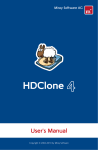
The illustration shows the schematic user interface with its basic elements.
(1) Menu bar
(2) Document group
(3) Toolbars
(4) Tool windows
(5) Status bar
You can call up many commands by using the corresponding menu. Your
software's menu bar can be configured to suit your requirements. Use the Tools
> Customization > Start Customize Mode... command to add menus, modify, or
delete them.
The document group contains all loaded documents. These can be of all
supported document types.
When you start your software, the document group is empty. While you use your
software it gets filled - e.g., when you load or acquire images, or perform various
image processing operations to change the source image and create a new one.
Commands you use frequently are linked to a button providing you with quick
and easy access to these functions. Please note, that there are many functions
which are only accessible via a toolbar, e.g., the drawing functions required for
annotating an image. Use the Tools > Customization > Start Customize Mode...
command to modify a toolbar's appearance to suit your requirements.
Tool windows combine functions into groups. These may be very different
functions. For example, in the Properties tool window you will find all the
information available on the active document. In contrast to dialog boxes, tool
windows remain visible on the user interface as long as they are switched on.
That gives you access to the settings in the tool windows at any time.
The status bar contains a large amount of information, e.g., a brief description of
each function. Simply move the mouse pointer over the command or button for
this information.
00108
6
User interface
2.2.
Layouts
To switch backwards and forwards between different layouts, click on the righthand side in the menu bar on the name of the layout you want, or use the View >
Layout command.
Which predefined
layouts are there?
For important tasks several layouts have already been defined. The following
layouts are available:
Acquiring images ("Acquisition" layout)
Viewing and processing images ("Processing" layout)
Measuring images ("Count and Measure" layout)
Generating a report ("Reporting" layout )
In contrast to your own layouts, predefined layouts can't be deleted. Therefore,
you can always restore a predefined layout back to its originally defined form. To
do this, select the predefined layout, and use the View > Layout > Reset Current
Layout command.
What is a layout?
Your software's user interface is to a great extent configurable, so that it can
easily be adapted to meet the requirements of individual users or of different
tasks. You can define a so-called "layout" that is suitable for the task on hand. A
"layout" is an arrangement of the control elements on your monitor that is optimal
for the task on hand. In any layout, only the software functions that are important
in respect to this layout will be available.
Example: The Camera Control tool window is only of importance when you
acquire images. When instead of that, you want to measure images, you don't
need that tool window.
That's why the "Acquisition" layout contains the Camera Control tool window,
while in the "Count and Measure" layout it's hidden.
Which elements of the
user interface belong to
the layout?
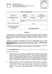
The illustration shows you the elements of the user interface that belong to the
layout.
(1) Toolbars
(2) Tool windows
(3) Status bar
(4) Menu bar
The layout saves the element's size and position, regardless of whether they
have been shown or hidden. When, for example, you have brought the Windows
toolbar into a layout, it will only be available for this one layout.
00013
7
User interface
2.3.
Document group
The document group contains all loaded documents. These can be of all
supported document types. As a rule, the loaded documents are images.
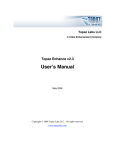
Appearance of the
document group
(1) Document group in the user interface
(2) Document bar in the document group
(3) Buttons in the document bar
(4) Navigation bar in the image window
(1) Document group in the user interface
You will find the document group in the middle of the user interface. In it you will
find all of the documents that have been loaded, and of course also all of the
images that have been acquired. Also the live-image and the images resulting
from, e.g., any image processing function, will be displayed there.
(2) Document bar in the document group
The document bar is the document group's header.
For every loaded document, an individual tab showing the document name will
be set up in the document group. Click the name of a document in the document
bar to have this document displayed in the document group. The name of the
active document will be shown in color. Each type of document is identified by its
own icon.
At the top right of each tab, a small [ x ] button is located. Click the button with
the cross to close the document. If it has not yet been saved, the Unsaved
Documents dialog box will open. You can then decide whether or not you still
need the data.
8
User interface
(3) Buttons in the document bar
At the top right of the document bar you will see several buttons.
Button with a hand
Click the button with a hand on it to extract the document group from the user
interface. In this way you will create a document window that you can freely
position or change in size.
If you would like to merge two document groups, click the button with the hand in
one of the two document groups. With the left mouse button depressed, drag the
document group with all the files loaded in it, onto an existing one.
Prerequisite: You can only position document groups as you wish when you are
in the expert mode. In standard mode the button with the hand is not available.
Arrow buttons
The arrow buttons located at the top right of the document group are, to begin
with, inactive when you start your software. The arrow buttons will only become
active when you have loaded so many documents that all of their names can no
longer be displayed in the document group. Then you can click one of the two
arrows to make the fields with the document names scroll to the left or the right.
That will enable you to see the documents that were previously not shown.
(4) Navigation bar in the image window
Multi-dimensional images have their own navigation bar directly in the image
window. Use this navigation bar to set or to change how a multi-dimensional
image is to be displayed on your monitor.
There are some other document types with their own navigation bar directly in
the image window. One example is a report instruction or an experiment plan.
00139 02072013
2.4.
Tool Windows
Tool windows combine functions into groups. These may be very different
functions. For example, in the Properties tool window you will find all the
information available on the active document.
Which tool windows are shown by default depends on the layout you have
chosen. You can, at any time, make specific tool windows appear and disappear
manually. To do so, use the View > Tool Windows command.
Manually displayed or hidden tool windows will be saved together with the layout
and are available again the next time you start the program. A return to the
original layout using the View > Layout > Reset Current Layout command will
have the result that only the tool windows that are defined by default for this
layout will be displayed.
Position of the tool windows
The user interface is to a large degree configurable. For this reason, tool
windows can be docked, freely positioned, or integrated in document groups.
Docked tool windows
Tool windows can be docked to the left or right of the document window, or
below it. To save space, several tool windows may lie on top of each other. They
are then arranged as tabs. In this case, activate the required tool window by
clicking the title of the corresponding tab below the window.
9
User interface
Freely positioned tool
windows
You can only position tool windows as you wish when you are in the expert
mode.
You can at any time float a tool window. The tool window then behaves exactly
the way a dialog box does. To release a tool window from its docked position,
click on its header with your left mouse button. Then, while keeping the left
mouse button depressed, drag the tool window to wherever you want it.
Integrating a tool
window into a
document group
You can only add tool windows to a document group when you are in the expert
mode.
You can integrate certain tool windows in the document group, for example, the
File Explorer tool window. To do this, use the Document Mode command. To
open a context menu containing this command, rightclick any tool window's
header.
The tool window will then act similarly to a document window, e.g., like an image
window.
Use the Tool Window Mode command to float a tool window back out of the
document group. To open a context menu containing this command, rightclick
any tool window's header.
Buttons in the header
In the header of every tool window, you will find the three buttons Help, Auto
Hide and Close.
Click the Help button to open the online help for the tool window.
Click the Auto Hide button to minimize the tool window.
Click the Close button to hide the tool window. You can make it reappear at any
time, for example, with the View > Tool Windows command.
Context menu of the header
To open a context menu, rightclick a tool window's header. The context menu
can contain the Enable Auto Hide, Document Mode, and Transparency
commands. Which commands will be shown, depends on the tool window.
Additionally, the context menu contains a list of all of the tool windows that are
available. Every tool window is identified by its own icon. The icons of the
currently displayed tool windows will appear clicked. You can recognize this
status by the icon's background color.
Use this list to make tool windows appear.
00037
10
User interface
2.5.
Image window views
When working with multi-dimensional images you can choose between different
views of the image in the image window. Multi-dimensional images have their
own navigation bar directly in the image window. Click the small arrow next to the
last button on this navigation bar to open a menu with commands you can use
with image window views. In it, you can select the image window view you want
and also edit the settings for some views.
The button's
appearance
Overview - Image
window views
This button is configured in such a way that you can switch backwards and
forwards exactly between two different views simply by clicking it once.
Click the button to switch to the image window view that is currently shown as an
icon on the button. Every image window view has its own icon.
The button always shows the image window view that was previously selected.
For example, when you switch from the single frame view to the Slice View
image window view, the button will automatically change its appearance to show
the icon for the single frame view, making it possible for you to immediately
switch back to that view.
Single Frame View
By default you will find yourself in the single view. In the single frame view, only
one image will be shown in the image window.
Tile View
Use the tile view to attain an overview of all of the individual images that make up
a multi-dimensional image. In this view, you can also select individual images.
Slice View
Use the Slice View image window view, to look at any cross sections of an image
series you want. The Slice View tool window offers you numerous possibilities for
configuring this view.
Voxel View
You can display a Z-stack as a 3D object. To do so, use the Voxel View image
window view, and the Voxel View tool window.
Projection Views
For image series, e.g. Z-stacks and time stacks, a single projection image can be
calculated from all of the frames that is representative for the whole multidimensional image. The available projection images differ in the calculation
algorithm. For example, if you use the maximum intensity projection you will,
from all frames, only see the pixels with the highest intensity values.
EFI Projection
For Z-stacks an EFI projection is available. The EFI projection uses a series of
differently focused separate images ("Focus series") to calculate a resulting
image ("EFI image"), that is focused in all of its parts.
00354
11
User interface
2.6.
Working with documents
You can choose from a number of possibilities when you want to open, save, or
close documents. As a rule, these documents will be images. In addition, your
software supports some other document types. You will find a list of supported
documents in the online help.
Saving documents
You should always save important documents immediately following their
acquisition. You can recognize documents that have not been saved by the star
icon after the document's name.
There are a number of ways in which you can save documents.
1. To save a single document, activate the document in the document group
and use the File > Save As... command.
2. Use the Documents tool window.
Select the desired document and use the Save command in the context
menu. For the selection of documents, the standard MS-Windows
conventions for multiple selection are valid.
3. Use the Gallery tool window.
Select the desired document and use the Save command in the context
menu. For the selection of documents, the standard MS-Windows
conventions for multiple selection are valid.
4. Save your documents in a database. That enables you to store all manner of
data that belongs together in one location. Search and filter functions make it
quick and easy to locate saved documents.
Autosave and close
1. When you exit your software, all data that has not yet been saved will be
listed in the Unsaved Documents dialog box. This gives you the chance to
decide which document you still want to save.
2. With some acquisition processes, the acquired images will be automatically
saved after the acquisition has finished.
3. You can also configure your software in such a way that all images are saved
automatically after image acquisition. To do so, use the Acquisition Settings
> Saving dialog box.
Here, you can also configure your software in such a way that all images are
automatically saved in a database after the image acquisition.
Closing documents
There are a number of ways in which you can close documents.
1. Use the Documents tool window.
Select the desired documents and use the Close command in the context
menu. For the selection of documents, the standard MS-Windows
conventions for multiple selection are valid.
2. To close a single document, activate the document in the document group
and use the File > Close command. Alternatively, you can click the button
with the cross [ x ]. You can find this button at the top right of the document
tab located next to the document name.
3. Use the Gallery tool window.
Select the desired documents and use the Close command in the context
menu. For the selection of documents, the standard MS-Windows
conventions for multiple selection are valid.
12
User interface
Closing all documents
Closing a document
immediately
To close all loaded documents use the Close All command. You will find this
command in the File menu, and in both the Documents and the Gallery tool
window's context menu.
To close a document immediately without a query, close it with the [Shift] key
depressed. Data you have not saved will be lost.
Opening documents
There are a number of ways in which you can open or load documents.
1. Use the File > Open... command.
2. Use the File Explorer tool window.
To load a single image, double click on the image file in the File Explorer tool
window.
To load several images simultaneously, select the images and with the left
mouse button depressed, drag them into the document group. For the
selection of images the standard MS-Windows conventions for multiple
selection are valid.
3. Drag the document you want, directly out of the MS-Windows Explorer, onto
your software's document group.
4. To load documents from a database into the document group, use the
Database > Load Documents... command. You can find more information in
the online help.
Generating a test
image
If you want to get used to your software, then sometimes any image suffices to
try out a function.
Press [Ctrl + Shift + Alt + T] to generate a color test image.
With the [Ctrl + Alt + T] shortcut, you can generate a test image that is made up
of 256 gray values.
Activating documents in the document group
There are several ways to activate one of the documents that has been loaded
into the document group and thus display it on your monitor.
1. Use the Documents tool window. Click the desired document there.
2. Use the Gallery tool window. Click the desired document there.
3. Click the title of the desired document in the document group.
4. To open a list with all currently loaded documents, use the [Ctrl + Tab]
shortcut. Left click the document that you want to have displayed on your
monitor.
5. Use the keyboard shortcut [Ctrl + F6] or [Ctrl + Shift + F6], to have the next
document in the document group displayed. With this keyboard shortcut you
can display all of the loaded documents one after the other.
6. In the Window menu, you will find a list of all of the documents that have
been loaded. Select the document you want from this list.
13
User interface
Attaching a document to an e-mail
1. Load the documents you want to attach to your e-mail.
2. Use the File > Send E-mail... command.
3. Check whether all documents you want to attach are selected.
4. Click the Send button to generate an e-mail with the selected documents
included as attachments.

You will receive a warning message if the sum of file sizes of all
documents exceeds the maximum permitted size.

A new e-mail form will be opened by your e-mail program. Your e-mail
program does not have to be already running for this to happen. The email contains all of the selected image and document files as
attachments.
As long as the e-mail form remains open, you cannot use your software
or your e-mail program. The e-mail form cannot be minimized, no can
other e-mails be generated, nor can you read any incoming e-mails. You
can't close the Send E-mail dialog box nor continue working.
5. Enter the recipient’s address and your message and then send off your email.
00143 02072013
14
Configuring the system
3.
Configuring the system
Why do you have to
configure the system?
After successfully installing your software you will need to first configure your
image analysis system, then calibrate it. Only when you have done this will you
have made the preparations that are necessary to ensure that you will be able to
acquire high quality images that are correctly calibrated. When you work with a
motorized microscope, you will also need to configure the existing hardware, to
enable the program to control the motorized parts of your microscope.
Process flow of the configuration
To set up your system, the following steps are necessary:
Selecting the camera and the microscope
Specifying which hardware is available
Configuring the interfaces
Configuring the specified hardware
Calibrating the system
Selecting the camera
and the microscope
The first time you start your software after the installation has been made, a
quick configuration with some default settings will be made. In this step you need
only to specify the camera and microscope types, in the Quick Device Setup
dialog box. The microscope will be configured with a selection of typical
hardware components.
Specifying which
hardware is available
Your software has to know which hardware components your microscope is
equipped with. Only these hardware components can be configured and
subsequently controlled by the software. In the Acquire > Devices > Device List
dialog box, you select the hardware components that are available on your
microscope.
You can find more information on this dialog box in the online help.
If you use a preset configuration that was offered in the Quick Device Setup
dialog box, check now whether your system is really equipped with the hardware
components that are defined in the configuration.
Configuring the
interfaces
Configuring the
specified hardware
Calibrating the system
Use the Acquire > Devices > Interfaces command, to configure the interfaces
between your microscope or other motorized components, and the PC on which
your software runs.
If you use a preset configuration that was offered in the Quick Device Setup
dialog box, you can skip this step.
Usually various different devices, such as a camera, a microscope and/or a
stage, will belong to your system. Use the Acquire > Devices > Device Settings...
dialog box to configure the connected devices so that they can be correctly
actuated by your software.
When all of the hardware components have been registered with your software
and have been configured, the functioning of the system is already ensured.
However, it's only really easy to work with the system and to acquire top quality
images, when you have calibrated your software. The detailed information that
helps you to make optimal acquisitions, will then be available.
Your software offers a wizard that will help you while you go through the
15
Configuring the system
individual calibration processes. Use the Acquire > Calibrations... command to
start the software wizard.
You can find more information on the individual dialog boxes in the online help.
About the system configuration
When do you have to
configure the system?
You will only need to completely configure and calibrate your system anew when
you have installed the software on your PC for the first time, and then start it.
When you later change the way your microscope is equipped, you will only need
to change the configuration of certain hardware components, and possibly also
recalibrate them.
Switching off your
operating system's
hibernation mode
When you use the MS-Windows Vista operating system: Switch the hibernation
mode off.
1. To do so, click the Start button located at the bottom left of the operating
system's task bar.
2. Use the Control Panel command.
3. Open the System and Maintenance > Power Options > Change when the
computer sleeps window.

Here, you can switch off your PC's hibernation mode.
When you use the MS-Windows 7 operating system: Switch off your PC's power
saving options and make sure that your PC does not automatically goes to
hibernation mode.
1. To do so, click the Start button located at the bottom left of the operating
system's task bar.
2. Click Control Panel, System and Security, and then click Power Options.
3. On the Select a power plan page, click Change plan settings.
4. On the Change settings for the plan page, click Change advanced power
settings.

Here, you can switch off your PC's power saving and hibernation mode.
00159
16
Acquiring single images
4.
Acquiring single images
4.1.
Acquiring a single image
You can use your software to acquire high resolution images in a very short
period of time. For your first acquisition you should carry out these instructions
step for step. Then, when you later make other acquisitions, you will notice that
for similar types of sample many of the settings you made for the first acquisition
can be adopted without change.
1. Switch to the Acquisition layout. To do this, use, e.g., the View > Layout >
Acquisition command.

You can find the Microscope Control (1) toolbar at the upper edge of the
user interface, right below the menu bar.
To the left of the document group, you see the Camera Control (2) tool
window.
Selecting an objective
2. On the Microscope Control toolbar, click the button with the objective that
you use for the image acquisition.
Switching on the liveimage
3. In the Camera Control tool window, click the Live button.

You can find more information in the online help.

The live-image (3) will now be shown in the document group.
4. Go to the required specimen position in the live-image.
Setting the image
quality
5. Bring the sample into focus. The Focus Indicator toolbar is there for you to
use when you are focusing on your sample.
6. Check the color reproduction. If necessary, carry out a white balance.
7. Check the exposure time. You can either use the automatic exposure time
function, or enter the exposure time manually.
8. Select the resolution you want.
Acquiring and saving
an image
9. In the Camera Control tool window, click the Snap button.

The acquired image will be shown in the document group.
10. Use the File > Save As... command to save the image. Use the
recommended TIF file format.
00027 18012012
17
Acquiring single images
4.2.
Behavior of the live window
The behavior of the live window depends on the acquisition settings in the
Acquisition Settings > Acquisition > General dialog box.
Prerequisite
For the following step-by-step instructions, the Keep document when live is
stopped option is selected and the Create new document when live is started
check box is cleared.
Switching the live-image on and off without acquiring an
image
1. Make the Camera Control tool window appear. To do this, use, e.g., the View
> Tool Windows > Camera Control command.
2. Click the Live button in the Camera Control tool window.

A temporary live window named "Live (active)" will be created in the
document group.

The live-image will be shown in the live window.

You can always recognize the live modus by the changed look of the
Live button in the Camera Control tool window.
3. Click the Live button again.

The live mode will be switched off.

The active live image will be stopped.

The live window's header will change to "Live (stopped)". You can save
the stopped live-image located in the live window just as you can every
other image.
The live window may look similar to an image window, but it will be handled
differently. The next time you switch on the live mode, the image will be
overwritten. Additionally, it will be closed without a warning message when your
software is closed.
Switching to the live-image and acquiring an image
1. Make the Camera Control tool window appear. To do this, use, e.g., the View
> Tool Windows > Camera Control command.
2. Click the Live button in the Camera Control tool window.

A temporary live window named "Live (active)" will be created in the
document group.

The live-image will be shown in the live window.

You can always recognize the live modus by the changed look of the
Live button in the Camera Control tool window.
3. Click the Snap button.

The live mode will be switched off. The live window's header will change
to "Live (stopped)".

At the same time, a new image document will be created and displayed
in the document group. You can rename and save this image. If you
have not already saved it when you end your software, you will be asked
if you want to do so.
18
Acquiring single images
Displaying the live-image and the acquired images
simultaneously
Task
You want to view the live-image and the acquired images simultaneously. When
you do this, it should also be possible to look through the acquired images
without having to end the live mode.
1. Close all open documents.
2. Open the Acquisition Settings > Acquisition > General dialog box.
To do so, click, e.g., the Acquisition Settings
Control tool window.
button on the Camera
3. There, make the following settings:

Choose the Keep document when live is stopped option.

Clear the Create new document when live is started check box.

Select the Continue live after acquisition check box.
4. Switch to the live mode. Acquire an image, then switch the live mode off
again

Both of the image windows "Live (stopped)" and "Image_<Serial No.>"
are now in the document group.

The "Live (stopped)" image window is active. That's to say, right now you
see the stopped live-image in the document group. In the document bar,
the Name "Live (stopped)" is highlighted in color.
5. Split the document group, to have two images displayed next to each other.
That's only possible when at least two images have been loaded. That's why
you created two images in the first step.
6. Use the Window > Split/Unsplit > Split/Unsplit Document Group (Left)
command.

This command creates a new document group to the left of the current
document group. In the newly set up document group the active
document will be automatically displayed. Since in this case, the active
document is the stopped live-image, you will now see the live window on
the left and the acquired image on the right.
7. Start the live mode.

In the document group, the left window will become the live window Live
(active)". Here, you see the live-image.
8. Activate the document group on the right. To do so, click, for example, the
image displayed there.
9. Click the Snap
button.

The acquired image will be displayed in the active document group. In
this case, it's the document group on the right.

After the image acquisition has been made, the live-image will
automatically start once more, so that you'll then see the live-image
again on the left.

While the live-image is being shown on the left, you can switch as often
as you want between the images that have up till then been acquired.
19
Acquiring single images
You can set up your software's user interface in such a way that you can view the
live-image (1) and the images that have up till then been acquired (2), next to
one another.
00181 25072011
4.3.
Acquiring HDR images
HDR stands for High Dynamic Range. Dynamic range relates to the capacity of
cameras or software to display both bright and dark image segments.
Before acquiring an HDR image, the necessary exposure range needs to be
determined for the current sample. The exposure range is made up of a minimum
and maximum exposure time as well as several exposure times between them. A
recently determined exposure range will continue to be used for all HDR images
until you let your software determine the exposure range anew. It is irrelevant
whether the exposure range had been determined automatically or manually.
If you are acquiring several images of the same or similar parts of a sample, you
don't need to determine the exposure range each time. If you change the sample
or adjust settings on the microscope, it is recommended to determine the
exposure range anew (either automatically or manually).
Acquiring an HDR image with a manually determined exposure
range
With this procedure, you set the minimum and maximum exposure time in the
Camera Control tool window yourself. Your software guides you through the
process with relevant message boxes. How much the exposure time is adjusted
by is determined by your software with regards to the minimum and maximum
exposure time.
Preparations
1. Switch to the Acquisition layout. To do this, use, e.g., the View > Layout >
Acquisition command.
2. On the Microscope Control toolbar, click the button with the objective that
you want to use for the acquisition of the HDR image.
3. Switch to the live mode, and select the optimal settings for your acquisition,
in the Camera Control tool window. Carry out a white balance. Choose an
approximate exposure time.
4. Search for the part of the sample which you want to acquire an HDR image
of. This should be a position which has such significant differences in
brightness that not all segments can be shown with optimal lighting.
5. Finish the live mode.
20
Acquiring single images
Acquiring an HDR
image
6. In the Camera Control tool window, select the Activate HDR check box.

In the upper part of the tool window, the Snap button changes to the
HDR button.
7. In the Determine exposure range group, click the Manual... button to define
the exposure range for this acquisition anew.

The Determine exposure range message box appears. It prompts you to
reduce the exposure time so far that enough image details can be
recognized in the bright image segments and no segments are
overexposed.
8. Change the exposure time in the Exposure group, which is part of the
Camera Control tool window. Make sure that the Manual option is chosen.
You can change the value by using the slide control or by entering an
exposure time with the keyboard and pressing the [Enter] key. Check the live
image on display. Once the bright image segments are no longer
overexposed, click the OK button in the Determine exposure range message
box.

By doing so, you have determined the lower limit of the exposure range
(=the shortest exposure time).
9. Now, the Determine exposure range message box prompts you to raise the
exposure time so high that the dark image segments are no longer
underexposed. Change the exposure time in the Exposure group, which is
part of the Camera Control tool window. Check the live image on display.
Once the dark image segments are bright enough, click the OK button in the
Determine exposure range message box.

By doing so, you have determined the upper limit of the exposure range
(=the longest exposure time).
10. Click the HDR button in the Camera Control tool window to start the image
acquisition.

The image acquisition will begin. Pay attention to the progress bar
. It shows
located in the status bar
how long the acquisition has taken and the total acquisition time. The
progress bar contains the Cancel button, which you can use to stop the
current image acquisition.

After the acquisition has been completed the HDR image will be shown
in the document group.
11. Check the image. If you want to change the settings (to use a different
algorithm for the output rendering, for example), open the Acquisition
Settings dialog box. Select the Acquisition > HDR option in the tree view.

You can find more information on this topic in the online help.
12. If you don't want to change any settings, use the File > Save As... command
to save the image. Use the recommended TIF or VSI file format.

These are the only formats which also save all the image information
including the HDR entries together with the image. In this way, you can
see, e.g., whether or not an image was acquired using HDR. Open the
Properties tool window, and look at the data in the Camera group.
21
Acquiring single images
Acquiring more HDR images without setting the exposure
range anew
If you have just acquired HDR images of the same or a similar sample, as a rule,
it is not necessary to determine the dynamic range anew. In this case, you have
already completed the preparations for acquisition (such as carrying out a white
balance) and set the HDR image acquisition settings correctly (such as choosing
the optimal algorithm used for output rendering) anyway.
In such circumstances, acquiring an HDR image is especially easy. Do the
following:
1. In the Camera Control tool window, select the Activate HDR check box.
2. Click the HDR button in the Camera Control tool window to start the image
acquisition.

The image acquisition will begin. After the acquisition has been
completed the HDR image will be shown in the document group.
3. Check the image before saving it.

This step can be left out if your software is configured to import images
into a database directly after acquisition.
07500 27122011
22
Acquiring multi-dimensional images
5.
Acquiring multi-dimensional
images
What is a multi-dimensional image?
You can combine a series of individual images into one image. You can, e.g.,
assemble separate images that belong to different color channels. Depending on
how the frames differ, the multi-dimensional image that results from their
combination will also vary.
A standard image is two dimensional. The position of every pixel will be
determined by its X- and Y-values. Fluorescence color, time and Z-position of the
microscope stage are the possible additional dimensions of a multi-dimensional
image.
A multi-channel image as a rule, shows a sample that has been marked with
several different fluorochromes. The multi-channel image is made up of a
combination of the individual fluorescence images.
In a time stack all frames have been acquired at different points of time. A
time stack shows you how an area of a sample changes with time. You can
play back a time stack just as you do a movie.
A Z-stack contains frames acquired at different focus positions. You need a Zstack, for instance, for the calculation of an EFI image.
Image containing
several dimensions
The different multi-dimensional images can be arbitrarily combined. A multichannel time stack, for instance, incorporates several color channels. Every color
channel incorporated in the image is reproduced with its own time stack.
Navigation bar in the
image window
The multi-dimensional images have their own navigation bar directly in the image
window. Use this navigation bar to define how a multi-dimensional image is to be
displayed in the image window.
00009
5.1.
Overview - Acquisition processes
Your software offers a wide range of different acquisition processes.
Note: Your software is available in a variety of versions. This online help contains
the description of all acquisition processes. For this reason, it can happen that
your software version doesn't have some of the acquisition processes described
here.
Basic acquisition
processes
Complex acquisition
processes
23
Acquiring multi-dimensional images
Basic acquisition processes
Use the Camera Control tool window to acquire images and movies.
Acquisition process Snapshot
You can use your software to acquire high resolution images in a very short
period of time.
Acquisition process Movie
You can use your software to record a movie. When you do this, your camera will
acquire as many images as it can within an arbitrary period of time. The movie
will be saved as a file in the AVI format. You can use your software to play it
back.
Complex acquisition processes
Use the Process Manager tool window to handle complex acquisition processes.
Acquisition process Time Lapse
With the automatic acquisition process Time Lapse you acquire a series of
frames one after the other. This series of individual images makes up a time
stack. A time stack shows you how an area of a sample changes with time. You
can play back a time stack just as you do a movie.
You can combine the Time Lapse acquisition process with other acquisition
processes. If you software supports the Multi Channel acquisition process, use,
e.g., the Time Lapse acquisition process to acquire a multi-channel time stack.
If your microscope stage is equipped with a motorized Z-drive, when you
acquire a time stack you can use the autofocus. You'll find a description of the
individual settings along with the description of the acquisition process.
Acquisition process Z-Stack
Use the automatic acquisition process Z-Stack to acquire a Z-stack. A Z-stack
contains frames acquired at different focus positions. That is to say, the
microscope stage was located in a different Z-position for the acquisition of each
frame.
Alternatively, you can also acquire an EFI image with the Z-Stack acquisition
process. Then a resulting image (EFI image) with a practically unlimited depth of
focus is automatically calculated from the Z-stack that has been acquired. Such
an image is focused throughout all of its segments. EFI is the abbreviation for
Extended Focal Imaging.
You can combine the Z-Stack acquisition process with other acquisition
processes.
If you software supports the Multi Channel acquisition process, you can combine
the Z-Stack acquisition process with the multi channel acquisition to acquire a
multi-channel Z-stack.
Acquisition process XY-Positions / MIA
You can only use this acquisition process when your microscope is equipped
with a motorized XY-stage. With this acquisition process you can carry out one or
more automatic acquisition processes at different positions on the sample or
acquire a stitched image of a larger sample position.
If your microscope stage is equipped with a motorized Z-drive, you can use
the autofocus for this acquisition process. You'll find a description of the
individual settings along with the description of the acquisition process.
24
Acquiring multi-dimensional images
Acquisition process Multi Channel
With the automatic acquisition process Multi Channel you acquire a multi-channel
fluorescence image.
You can combine, e.g., the Multi Channel acquisition process with the Z-stack
acquisition process to acquire a multi-channel Z-stack.
Note: When you use the DP80 camera, please note the following restriction.
When you acquire a transmitted light image simultaneously with a multi-channel
fluorescence image, the Multi Channel acquisition process can't be combined
with another acquisition process, for example the Z-stack acquisition process.
This restriction protects the camera from being damaged by permanently toggling
between the two CCDs the camera provides.
Acquisition process Instant EFI
Use the manual acquisition process Instant EFI to acquire an EFI image at the
camera's current position, that is sharply focused all over.
Acquisition process Manual MIA
When you use the Manual MIA acquisition process, you move the stage
manually in such a way that different, adjoining sample areas are shown. With
this acquisition process, you combine all of the images that are acquired, directly
during the acquisition, just like a puzzle, into a stitched image. The stitched
image will display a large sample segment in a higher X/Y-resolution than would
be possible with a single acquisition.
Combination of several acquisition processes
You can combine several automatic acquisition processes. To do so, click the
corresponding button for each acquisition process you require.
Note: Which automatic acquisition processes you can combine with each other,
depends on your software.
The order of the automatic acquisition processes in the Process Manager tool
window (from left to right) corresponds to the order in which the acquisition
processes were carried out.
Examples
When you combine the two acquisition processes Multi Channel and Z-Stack, a
complete multi-channel image will be acquired at every focus position. The Multi
Channel acquisition process will then be carried out first. Only after this has been
done, will the stage's Z-position be changed, and another multi-channel image
acquired.
When you combine the two acquisition processes Z-Stack and XY-Positions /
MIA to acquire a Z-stack at several positions on your sample, to begin with, the
complete Z-stack at the first position will be acquired. When that has been done,
your system will move to the next position, and will acquire the next Z-stack etc..
00442 13012011
25
Acquiring image series
6.
Acquiring image series
With your software you can acquire time stacks, movies, and Z-stacks.
6.1.
Acquiring time stacks
What is a time stack?
You can combine a series of individual images into one image. In a time stack all
frames have been acquired at different points of time. A time stack shows you
how an area of a sample changes with time. You can play back a time stack just
as you do a movie.
A standard image is two dimensional. The position of every pixel will be
determined by its X- and Y-values. With a time stack, the time when the image
was acquired is an additional piece of information or "dimension" for each frame.
The frames making up a time stack can be 8-bit gray-value images, 16-bit grayvalue images or 24-bit true-color images.
Note: A time stack can also be an AVI video. You can load and play back the AVI
file format with your software.
How do I recognize a
time stack?
You can immediately recognize the different image types by the icon which
appears in front of the image name in the document group, or in the Documents
tool window. When it is a time stack, this icon will be supplemented by a small
clock. A time stack that is made up of true-color images has, e.g., this icon
.
In the Properties tool window, you can use the Frame Count entry to find out how
many individual images are contained in any given image.
A time stack will automatically have its own navigation bar directly in the image
window. Use this navigation bar to browse through the frames making up a time
stack, or to play back the time stack like a movie.
You can find more information on the navigation bar in the online help.
Creating time stacks
There are different ways in which you can generate a time stack.
To acquire a time stack, use one of the two acquisition processes Time Lapse or
Movie.
Use the Image > Combine Frames… command, to have several individual
images combined into a time stack. A description of the Combine Frames dialog
box can be found in the online help.
Displaying time stacks
A time stack contains much more data than can be displayed on your monitor.
A time stack will automatically have its own navigation bar directly in the image
window. Use this navigation bar to determine which of the frames from a time
stack is to be displayed on your monitor. You can also play back a time stack just
as you would a movie.
You can find more information on the navigation bar in the online help.
Alternatively, you can also use the Dimension Selector tool window to determine
how a time stack is to be displayed on your monitor, or to change this.
Hiding the navigation
bar
You can also hide the navigation bar. To do this, use the Tools > Options...
command. Select the Images > General entry in the tree view. Clear the Show
image navigation toolbar check box.
26
Acquiring image series
Saving time stacks
When you save time stacks, you will, as a rule, use the VSI file format. Only
when you use this file format is there no limit to the size a time stack can be.
When you save smaller time stacks, you can also use the TIF or the AVI file
format. With any other file format you will lose most of the image information
during saving. To do so, use the File > Save As... command.
Converting time stacks
Use the Image > Separate > Time Frames menu command to have a time stack
broken down into selected individual images.
It is possible that, within a time stack, only a short period of time interests you.
Use the Extract command to create a new time stack that only contains a
selection of frames, from an existing time stack. In this way, you will reduce the
number of frames within a time stack to only those that interest you. You will find
this command in the context menu in the tile view for time stacks. You can find
more information on this command in the online help.
When you save a time stack in another file format as TIF or VSI, the time stack
will also be converted. The time stack will then be turned into a standard truecolor image. This image shows the frame that is at that moment displayed on the
monitor.
Processing time stacks
Image processing operations, e.g., a sharpen filter, affect either the whole image
or only a selection of individual images. You will find most of the image
processing operations in the Process menu. You can find more information on
working with image processing functions in the online help.
The dialog box that is opened when you use an image processing operation is
made up in the same way for every operation. In this dialog box, select the Apply
on > Selected frames and channels option to determine that the function only
affects the selected frames.
Select the Apply on > All frames and channels option, to process all of the
individual images.
Select the individual images that you want to process, in the tile view. You can
find more information on this image window view in the online help. Look through
the thumbnails and select the images you want to process. In the tile view, the
standard MS-Windows conventions for multiple selection are valid.
An image processing operation does not change the source image's dimensions.
The resulting image is, therefore, comprised of the same number of separate
images as the source image.
00011
Time Lapse / Movie
Both the "Time Lapse" and the "Movie" acquisition processes document the way
a sample changes with time. What is the difference between the two processes?
When is it better for me
to acquire a time stack?
Use the "Time Lapse" acquisition process in the following cases:



Use the "Time Lapse" acquisition process when processes that run
slowly are to be documented, e.g., where an acquisition is to be made
only every 15 minutes.
Use the "Time Lapse" acquisition process when, while the acquisition is
in progress, you want to see the frames that have already been acquired,
for example, to check on how an experiment is progressing. To do this,
click the Tile View
button in the navigation bar in the image window.
Use the "Time Lapse" acquisition process when you want to use those of
your software's additional functions that can only be saved in the VSI or
TIF file format.
For example, to measure objects, to insert drawing elements such as
arrows, or a text, or to have the acquisition parameters for the camera
and microscope that you've used, available at any time in the future.
27
Acquiring image series

Saving a time stack as
an AVI
When is it better for me
to acquire a movie?
Use the "Time Lapse" acquisition process when the important thing is to
achieve an optimal image quality, and the size of the file is no problem.
You can also save a time stack as an AVI file, at a later date. To do this, load the
time stack into the document group, select the File > Save as... command, and
select the AVI file type. Make, if necessary, additional settings in the Select AVI
Save Options dialog box.
Use the "Movie" acquisition process in the following cases:



Use the "Movie" acquisition process when processes that run very
quickly are to be documented (the number of acquisitions per second is
considerably higher with movies than with time stacks).
Use the "Movie" acquisition process when you want to give the movie to
third persons who do not have this software (AVI files can also be played
back with the MS Media Player).
Use the "Movie" acquisition process when keeping file sizes small is of
great importance.
00107
Recording a movie
You can use your software to record a movie. When you do this, your camera will
acquire as many images as it can within an arbitrary period of time. The movie
will be saved as a file in the AVI format. You can use your software to play it
back.
1. Switch to the "Acquisition" layout. To do this, use, e.g., the View > Layout >
Acquisition command.
Selecting an objective
2. On the Microscope Control toolbar, click the button with the objective that
you want to use for the movie acquisition.
Selecting the storage
location
3. In the Camera Control tool window's toolbar, click the Acquisition Settings
button.

The Acquisition Settings dialog box opens.
4. Select the Saving > Movie entry in the tree structure.
5. You have to decide how a movie is to be saved after the acquisition. Select
theFilesystem entry in the Automatic save > Destination list to automatically
save the movies you have acquired.

The Path field located in the Directory group shows the directory that will
currently be used when your movies are automatically saved.
6. Click the [...] button next to the Path field to alter the directory.

Selecting the
compression method
The AVI file format is preset in the File type list. This is a fixed setting
that cannot be changed.
7. Click the Options... button when you want to compress the AVI file in order to
reduce the movie's file size.
8. From the Compression list, select the M-JPEG entry and confirm with OK.
Please note: Compressing the movie is only possible if the selected
compression method (codec) has already been installed on your PC. If the
compression method has not been installed the AVI file will be saved
uncompressed.
The selected compression method must also be available on the PC that
is used for playing back the AVI. Otherwise the quality of the AVI may be
considerably worse when the AVI is played back.
9. Close the Acquisition Settings dialog box with OK.
28
Acquiring image series
Setting the image
quality
10. Switch to the live mode, and select the optimal settings for movie recording in
the Camera Control tool window. Pay special attention to setting the correct
exposure time.

This exposure time will not be changed during the movie recording.
11. Find the segment of the sample that interests you and focus on it.
Switching to the "Movie
recording" mode
12. Select the Movie recording check box (1). The check box can be found below
the Live button in the Camera Control tool window.

Starting movie
recording
Stopping movie
recording
The Snap button will be replaced by the Movie button.
13. Click the Movie button to start the movie recording.

The live-image will be shown and the recording of the movie will start
immediately.

In the status bar a progress indicator is displayed. At the left of the slash
the number of already acquired images will be indicated. At the right of
the slash an estimation of the maximum possible number of images will
be shown. This number depends on your camera's image size and
cannot exceed 2GB.

on the Movie button indicates that a movie is being
This icon
recorded at the moment.
14. Click the Movie button again to end the movie recording.

The first image of the movie will be displayed.

The navigation bar for time stacks will be shown in the document group.
Use this navigation bar to play the movie.

The software will remain in the "Movie recording" mode until you clear
the Movie recording check box once more.
Acquiring a time stack
In a time stack all frames have been acquired at different points of time. With a
time stack you can document the way the position on the sample changes with
time. To begin with, for the acquisition of a time stack make the same settings in
the Camera Control tool window as you do for the acquisition of a snapshot.
Additionally, in the Process Manager tool window, you have to define the time
sequence in which the images are to be acquired.
Task
You want to acquire a time stack over a period of 10 seconds. One image is to
be acquired every second.
1. Switch to the "Acquisition" layout. To do this, use, e.g., the View > Layout >
Acquisition command.
Selecting an objective
Setting the image
quality
2. On the Microscope Control toolbar, click the button with the objective that
you want to use for the image acquisition.
3. Switch to the live mode, and select the optimal settings for your acquisition,
in the Camera Control tool window. Pay special attention to setting the
29
Acquiring image series
correct exposure time. This exposure time will be used for all of the frames in
the time stack.
4. Choose the resolution you want for the time stack's frames, from the
Resolution > Snap/Process list.
5. Find the segment of the sample that interests you and focus on it.
Selecting the
acquisition process
6. Activate the Process Manager tool window.
7. Select the Automatic Processes option.
8. Click the Time Lapse button.

The button will appear clicked. You can recognize this status by the
button's colored background.

The [ t ] group will be automatically displayed in the tool window.
9. Should another acquisition process be active, e.g., Z-Stack, click the button
to switch off the acquisition process.

Selecting the
acquisition parameters
The group with the various acquisition processes should now look like
this:
10. Clear the check boxes Start delay and As fast as possible.
11. Specify the time that the complete acquisition is to take, e.g., 10 seconds.
Enter the value "00000:00:10" (for 10 seconds) in the Recording time field.
You can directly edit every number in the field. To do so, simply click in front
of the number you want to edit.
12. Select the radio button on the right-hand side of the field to specify that the
lock icon will
acquisition time is no longer to be changed. The
automatically appear beside the selected radio button.
13. Specify how many frames are to be acquired.
Enter e.g., 10 in the Cycles field.

The Interval field will be updated. It shows you the time that will elapse
between two consecutive frames.
Acquiring a time stack
14. Click the Start
button.

The acquisition of the time stack will start immediately.

The Start Process button changes into the Pause
this button will interrupt the acquisition process.

button will become active. A click on this button will stop
The Stop
the acquisition process. The images of the time stack acquired until this
moment will be preserved.

At the bottom left, in the status bar, the progress bar will appear. It
informs you about the number of images that are still to be acquired.

The acquisition has been completed when you can once more see the
button. A click on
button in the Process Manager tool window, and the progress
Start
bar has been faded out.

You will see the time stack you've acquired in the image window. Use the
navigation bar located in the image window to view the time stack. You
can find more information on the navigation bar in the online help.
30
Acquiring image series

The time stack that has been acquired will be automatically saved. The
storage directory is shown in the Acquisition Settings > Saving > Process
Manager dialog box. The preset file format is VSI.
Note: When other programs are running on your PC, for instance a virus
scanning program, it can interfere with the performance when a time stack is
being acquired.
00304 12012011
6.2.
Acquiring a Z-stack
What is a Z-stack?
You can combine a series of separate images into one image file. A Z-stack
contains frames acquired at different focus positions. A Z-stack is needed, e.g.,
for calculating an EFI image by the Process > Enhancement > EFI Processing...
command.
A standard image is two dimensional. The position of every pixel will be
determined by its X- and Y-values. With a Z-stack, the focus position or the
height of the sample is an additional item of information for every pixel.
The frames making up a Z-stack can be 8-bit gray-value images, 16-bit-grayvalue images or 24-bit-true-color images.
How do I recognize a Zstack?
You can immediately recognize a multi-dimensional image by its icon which
appears in front of the image name in the document group or in the Documents
tool window. When it is a Z-stack, this icon will be supplemented by a small Z
.
In the Properties tool window, you can use the Frame Count entry to find out how
many individual images are contained in any given image.
A Z-stack image will automatically have its own navigation bar directly in the
image window. Use this navigation bar to browse through the frames making up
a Z-stack, or to play back the Z-stack like a movie. You can find more information
on the navigation bar in the online help.
Creating a Z-stack
Displaying a Z-stack
There are different ways in which you can generate a Z-stack.

To acquire a Z-stack, use the "Z-Stack" acquisition process.

Use the Image > Combine Frames… command to have several separate
images combined into a Z-stack.
A Z-stack contains much more data than can be displayed on your monitor.
A Z-stack image will automatically have its own navigation bar directly in the
image window. Use this navigation bar to determine which of the frames from a
Z-stack is to be displayed on your monitor. You can also play back the Z-stack
just as you would a movie. A detailed description of the navigation bar can be
found in the online help.
Alternatively, you can also use the Dimension Selector tool window to define how
a Z-stack image is to be displayed on your monitor, or to change this.
Saving a Z-stack
Please note: Z-stacks can only be saved in the TIF or VSI file format. Otherwise
they loose a great deal of their image information during saving.
Converting a Z-stack
Use the Image > Separate > Z-Slices menu command, to have a Z-stack broken
down into selected frames.
31
Acquiring image series
It is possible that, within a Z-stack, only a short Z-range interests you. Use the
Extract command to create a new Z-stack that only contains selected frames,
from an existing Z-stack. In this way, you will reduce the number of frames within
a Z-stack to only those that interest you. You will find this command in the
context menu in the tile view for Z-stacks.
If you save a Z-stack in another file format as TIF or VSI, the Z-stack will
automatically be converted. The Z-stack will then be turned into a standard truecolor image. This image shows the frame that is at that moment displayed on the
monitor.
Processing a Z-stack
Image processing operations, e.g., a sharpen filter, affect either the whole image
or only a selection of individual images. You will find most of the image
processing operations in the Process menu. You can find more information on
working with image processing functions in the online help.
The dialog box that is opened when you use an image processing operation is
made up in the same way for every operation. In this dialog box, select the Apply
on > Selected frames and channels option to determine that the function only
affects the selected frames.
Select the individual images that you want to process, in the tile view. Click, e.g.,
this button
in the image window's navigation bar to switch to the tile view.
Look through the thumbnails and select the images you want to process. In the
tile view, the standard MS-Windows conventions for multiple selection are valid.
Select the Apply on > All frames and channels option to process all of the
individual images.
An image processing operation does not change the source image's dimensions.
The resulting image is, therefore, comprised of the same number of separate
images as the source image.
00012
Acquiring a Z-stack
A Z-stack contains frames acquired at different focus positions. That is to say,
the microscope stage was located in a different Z-position for the acquisition of
each frame.
Note: You can only use the Z-Stack acquisition process when your stage is
equipped with a motorized Z-drive.
Example: You want to acquire a Z-stack. The sample is approximately 50 µm
thick. The Z-distance between two frames is to be 2 µm.
1. Switch to the Acquisition layout. To do this, use, e.g., the View > Layout >
Acquisition command.
Selecting an objective
Setting the image
quality
2. On the Microscope Control toolbar, click the button with the objective that
you want to use for the image acquisition.
3. Switch to the live mode, and select the optimal settings for your acquisition,
in the Camera Control tool window. Pay special attention to setting the
correct exposure time. This exposure time will be used for all of the frames in
the Z-stack.
4. Search out the required position in the sample.
32
Acquiring image series
Selecting the
acquisition process
5. Activate the Process Manager tool window.
6. Select the Automatic Processes option.
7. Click the Z-Stack button.

The button will appear clicked. You can recognize this status by the
button's colored background.

The [ Z ] group will be automatically displayed in the tool window.
8. Should another acquisition process be active, e.g., Multi Channel, click the
button to switch off the acquisition process.
9. Select the Range entry in the Define list (1).
10. Enter the Z-range you want, in the Range field (2). In this example, enter a
little more than the sample's thickness (= 50 µm), e.g., the value 60.
11. In the Step Size (3) field, enter the required Z-distance, e.g., the value 2, for
a Z-distance of 2 µm. The value should roughly correspond to your
objective's depth of focus.

In the Z-Slices field (4) you will then be shown how many frames are to
be acquired. In this example 31 frames will be acquired.
12. Find the segment of the sample that interests you and focus on it. To do this,
use the arrow buttons (5). The buttons with a double arrow move the stage in
larger steps.
Selecting the
acquisition parameters
Set the acquisition parameters for the acquisition of a Z-stack in the Process
Manager tool window. Use the fields and buttons (1-4) for this.
Acquiring an image
13. Click the Start
button.

Your software now moves the Z-drive of the microscope stage to the
start position. The starting positions lies half of the Z-range deeper than
the stage's current Z-position.

The acquisition of the Z-stack will begin as soon as the starting position
has been reached. The microscope stage moves upwards step by step
and acquires an image at each new Z-position.
33
Acquiring image series

The acquisition has been completed when you can once more see the
button in the Process Manager tool window, and the progress
Start
bar has been faded out.

You can see the acquired Z-stack in the image window. Use the
navigation bar located in the image window to view the Z-stack. You can
find more information on the navigation bar in the online help.

The Z-stack that has been acquired will be automatically saved. You can
set the storage directory in the Acquisition Settings > Saving >
Process/Experiment dialog box. The preset file format is VSI.
Note: When other programs are running in the background on your PC, for
instance a virus scanning program, it can interfere with the performance when a
Z-stack is being acquired.
00367 10072013
34
Acquiring fluorescence images
7.
Acquiring fluorescence images
7.1.
Multi-channel image
What is a multi-channel image?
A multi-channel image combines a series of monochrome images into one
image. The multi-channel image usually shows a sample that has been stained
with several different fluorochromes. The multi-channel image is made up of a
combination of the individual fluorescence images. You can have the individual
fluorescence images displayed separately or also as a superimposition of all of
the fluorescence images.
At the top of the illustration you can see the individual fluorescence images (1).
Below, you can see the superimposition (2) of the separate fluorescence images.
The separate images'
image type
The separate images making up a multi-channel image can be 8-bit gray-value
images or 16-bit gray-value images.
Combination with a
times stack or Z-stack
A multi-channel image can be combined with a time stack or a Z-stack. A multichannel time stack, for instance, then incorporates several color channels. Every
color channel incorporated in the image is reproduced with its own time stack.
How do I recognize a multi-channel image?
You can immediately recognize a multi-channel image by this icon
which
appears in front of the image name in the document group or in the Documents
tool window.
In the Properties tool window, you can use the Channels entry to find out how
many channels are contained in any given image.
A multi-channel image will automatically have its own navigation bar, directly in
the image window. Use this navigation bar to set how a multi-channel image is to
be displayed in the image window, or to change this.
You can find more information on the navigation bar for multi-channel images in
the online help.
Creating multi-channel images
Your software offers you several ways of acquiring a multi-channel image.
Use the Multi Channel automatic acquisition process to acquire a multi-channel
image.
Use the Image > Combine Channels… command to have several separate
images combined into a multi-channel image.
35
Acquiring fluorescence images
Displaying multi-channel images
A multi-channel image contains much more data than can be displayed on your
monitor.
Using the navigation
bar
When you load a multi-channel image into your software, you'll see a navigation
bar in the image window, that provides you with access to all of the fluorescence
channels.



You can have the individual fluorescence images displayed separately or
also as a superimposition of all of the fluorescence images (1).
Should you have acquired a brightfield of the sample together with the
fluorescence images, you can make this brightfield appear or disappear
(2).
The individual fluorescence images are monochrome. For this reason,
you can change the color mapping however you like. You can display the
fluorescence channels in the fluorescence colors, use a pseudo color
table of your choice, or also display the original images (3).
Hiding the navigation
bar
You can also hide the navigation bar. To do this, use the Tools > Options...
command. Select the Images > General entry in the tree view. Clear the Show
image navigation toolbar check box.
Using the "Dimension
Selector" tool window
Alternatively, you can also use the Dimension Selector tool window to stipulate
how a multi-channel image is to be displayed on your monitor, or to change this.
There you can, for example, change the fluorescence colors for individual color
channels.
Saving multi-channel images
Please note: Multi-channel images can only be saved in the TIF or VSI file
format. Otherwise they loose a great deal of their image information during
saving.
Converting multi-channel images
Breaking down a multichannel image into its
color channels
Use the Separate command to have a multi-channel image broken down into
chosen color channels. The resulting images are still of the "multi-channel" type,
contain though, only one color channel.
There are several ways of accessing this command:



Reducing the color
channels in a multichannel image
Click the Separate Channels button in the Dimension Selector tool
window.
Use the Separate command from the Dimension Selector tool window's
context menu.
Use the Image > Separate > Channels menu command.
Use the Extract command to create a new multi-channel image that is made up
of fewer color channels than the source image.
36
Acquiring fluorescence images
Select all of the color channels you wish to retain, in the Dimension Selector tool
window. Then use the Extract command in the tool window's context menu.
Converting multichannel images while
saving them
When you save a multi-channel image in another file format as TIF or VSI, the
multi-channel image will also be converted. The multi-channel image then
becomes a standard 24-bit true-color image. This image will always show exactly
what is currently displayed on your monitor, that is to say, e.g., the
superimposition of all of the channels or possibly only one channel.
Processing multi-channel images
Image processing operations, e.g., a sharpen filter, affect either the whole image
or only a selection of individual images. You will find most of the image
processing operations in the Process menu. You can find more information on
working with image processing functions in the online help.
Select the frames that you want to process in the Dimension Selector tool
window. The channels you have selected will be highlighted in color in the tool
window.
The dialog box that is opened when you use an image processing operation is
made up in the same way for every operation. In this dialog box, select the Apply
on > Selected frames and channels option to determine that the function only
affects the selected frames.
Select the Apply on > All frames and channels option, to process all of the
individual images.
An image processing operation does not change the source image's dimensions.
The resulting image is, therefore, comprised of the same number of separate
images as the source image.
00010
7.2.
Before and after you've acquired a
fluorescence image
Before you acquire a fluorescence image
Defining observation
methods
Setting up the
microscope for the
acquisition of a
fluorescence image
Define observation methods for your color channels.
1. Use the View > Tool Windows > Microscope Control command to make the
Microscope Control tool window appear.

In the Objectives group, you will find the buttons you use to change
objectives.

In the Observation method group you will find a button for every
observation method that has been defined. Observation methods should
have been defined at least for brightfield and for every color channel.
2. Click the required objective's button.
3. Click the button for the observation method with the excitation that has the
longest excitation wavelength (e.g., Red)
Setting up the camera
for the acquisition of a
fluorescence image
.
1. Use the View > Tool Windows > Camera Control command to make the
Camera Control tool window appear.
37
Acquiring fluorescence images
2. Set the image resolution for the acquisition. With a high objective
magnification, you require a lower resolution.
For this purpose, select the required resolution from the Snap/Process list,
located in the Resolution group.
3. Reduce the image resolution in the live mode. When you use a higher
binning in the live mode, the frame rate will be reduced, which enables you to
focus better.
For this purpose, select an entry, e.g., with the supplement Binning 2x2, from
the Live/movie list, located in the Resolution group.
4. Should you work with a color camera: Switch on your camera's grayscale
mode. The Toggle RGB/Grayscale mode button should now look like this
. You can find this button on the Camera Control tool window's toolbar.
5. If it's possible to set different bit depths with your camera, click the Toggle
Bitdepth
Switching off the
corrections for
brightfield acquisitions
button to set the maximum bit depth.
1. Use the View > Toolbars > Calibrations command to have the Calibrations
toolbar displayed.
2. Switch off the white balance and the shading correction.
To do that, release these buttons
Focusing a
fluorescence sample
, if they are there and available.
1. Select the automatic exposure time.
2. In the Camera Control tool window, click the Live button.

Should the live-image be too dark, select a higher value in the Camera
Control > Exposure > Exposure compensation list.

Should the exposure time become longer than 300 ms, reduce it by
increasing the sensitivity or gain.
3. Bring the sample into focus.

In the camera's black & white mode, you can reduce the diffused light.
button, located in the Camera Control tool
Click the Online-Deblur
window's toolbar. You can then decide whether or not you want to apply
the deconvolution filter. It's possible that you might have to lengthen the
exposure time via the exposure time correction.
4. Finish the live mode. To do so, click the Live button in the Camera Control
tool window.
Setting the storage
location
Multi-channel images will be saved by default, as soon as the acquisition has
been completed. As file format, the VSI file format will be used.
1. Before you start the acquisition, specify where the file is to be saved.
2. To do this, click the Acquisition Settings
button, located in the Process
Manager tool window's toolbar. Select the Saving > Process Manager entry
in the tree view.

You will find the current directory in the Directory > Path field.
3. Click the [...] button next to the Path field, to change the directory into which
the image is to be saved after its acquisition.
38
Acquiring fluorescence images
After you've acquired a fluorescence image
Viewing a multi-channel
image
A multi-channel image is made up of the individual fluorescence images. You can
set which color channels, resp. combination of color channels, will be displayed
on your monitor. To do this, use the navigation bar in the image window.
Click a color field to make the channel appear or disappear. All of the color
channels that are at the moment displayed on your monitor will be identified by
an eye icon.
The navigation bar also offers you additional possibilities for changing the
appearance of the multi-channel image. You can find more information on the
navigation bar in the online help.
"Properties" tool
window
Saving multi-channel
images
Numerous acquisition parameters will be saved together with the image.
Use the View > Tool Windows > Properties command to make the Properties tool
window appear. In the Properties tool window, you will find that every color
channel has its own Channel information group. This contains the channel name,
the emission wavelength, the name of the observation method and the exposure
time.
The multi-channel image will be automatically saved. You can set the storage
directory in the Acquisition Settings > Saving > Process Manager dialog box. The
file format used is VSI.
For the VSI format, a JPEG compression of 90% is preset. You can change the
compression in the Acquisition Settings dialog box under Saving > Process
Manager > Automatic save > Options… .
00363
39
Acquiring fluorescence images
7.3.
Defining observation methods for the
fluorescence acquisition
Before you acquire a fluorescence image, you have to define observation
methods for your color channels. Usually, observation methods that you can
adapt for your microscope configuration, have already been predefined.
Prerequisite
The system has already been configured and calibrated. For this purpose, you
have to enter your hardware components in the Acquire > Devices > Device List
dialog box, and configure them in the Device Settings dialog box. To finalize this
action, calibrate your system by using the Acquire > Calibrations... command.
The tables that follow, contain example configurations for both motorized, and
not motorized microscopes. Only the hardware components that are relevant for
the acquisition of multi-channel fluorescence images are listed.
Example entries
Device List
Non-motorized
microscope
Motorized microscope
Microscope
Frame
<Name of your microscope>
BX51
BX61
Nosepiece
<Name of your nosepiece>
Manual Nosepiece
Motorized (UCB)
Mirror turret
<Name of your mirror turret>
Manual mirror turret
BX-RFAA
<Name of your controller for the
stage's Z-drive>
Not Motorized
Motorized (UCB)
<Name of the reflected light
shutter>
Manual Shutter
Motorized (UCB)
Lamp
<Name of your transmission
lamp>
Not used
UCB Halogen-Lamp
Condenser
<Name of your condenser>
Manual Condenser
U-UCD8A
Stage
Z-axis
Fluorescence/reflected light path
Shutter
Transmission light path
Device Settings
Entries
Nosepiece
<Your objectives>
Mirror turret
U-MNU, U-MWB, U-MWG
Condenser
The hardware components Aperture Stop and Top Lens are
additionally listed under the device settings.
For a position where there is no mirror cube, select the Free entry.
40
Acquiring fluorescence images
Defining the observation method for
transmission brightfield
Example: Hardware components in transmission brightfield: In transmission
brightfield, there is no fluorescence mirror cube in the light path. The reflected
light shutter is closed.
1. Use the Acquire > Devices > Device Customization... command. Activate the
Observation Methods tab.
2. Click the New Observation Method

button.
A dialog box, in which you can enter a name, will be opened.
3. Give the new observation method a name, then close the dialog box with OK.
You could name your observation method, e.g., MyBF.
Setting up the
mirror turret
4. Select the mirror turret in the Available components list.

In the central area of the dialog box, the settings for the hardware
components that have been selected, will be displayed.
5. In transmission brightfield, the mirror turret isn't allowed to contain a mirror
cube. Therefore, select the Adjust entry in the Status list, located in the
middle of the dialog box, and in the list that's below that one select the Free
entry.

For motorized
microscopes: Setting
up the condenser
For manual microscopes: Where a manual microscope is concerned, the
mirror turret can't be automatically moved to the position you want. For
this reason, when you use a manual microscope, you'll receive a
message that asks the user to make this setting manually.
This message will also appear when you are defining the observation
method. Confirm the message with OK.
6. Select the condenser.
Select the Adjust entry in the Status list, located in the middle of the dialog
box, and in the list that's below that one, the Free entry.
7. Select the hardware component Aperture Stop.
Select the Adjust entry in the Status list, located in the middle of the dialog
box. Enter "75%" in the field below that.
8. Select the hardware component Top Lens.
Select the Adjust per objective entry in the Status list.

In the middle of the Device Customization dialog box, you can now set
the top lens for each objective separately.

The top lens is only used for objectives with higher magnifications
(upwards of 10x) and is swung out for lower magnifications.
9. Specify for which objectives the top lens should be brought into the light path
and for which objectives it should be removed from the light path.
To do so, select the Use with this objective check box for all objectives.
In the Selected components list, each objective with a lower magnification
than 10x needs to show the Out status. If that isn't the case, click in the
middle of the dialog box on the Out button.
In the Selected components list, each objective with a higher magnification
than 10x or exactly 10x needs to show the In status. If that isn't the case,
click in the middle of the dialog box on the In button.
For motorized
microscopes: Switching
on the transmission
lamp
10. Select the transmission lamp. You will find this lamp in the Available
components list, under the Transmission entry.
11. Select the Adjust entry in the Status list, located in the middle of the dialog
box. Set 9 V for the lamp.
Use the button showing a small lamp to switch on the lamp.
41
Acquiring fluorescence images
Saving the observation
method

The button looks like this, if the lamp is switched on.

In the Selected components list, you can also see that the lamp for this
observation method will be switched on.
12. Click the OK button, to save the new observation method.

The Microscope Control tool window will then contain a new button with
this observation method's name.

You can now use the observation method in the Process Manager tool
window, for the acquisition of a multi-channel fluorescence image.
Defining observation methods for fluorescence
channels
Task
Summary
Define an observation method for the acquisition of a fluorescence image. It also
makes sense to do this when you don't work with a motorized microscope, since
then the acquired image will be automatically colored with the correct
fluorescence color.
The following hardware components belong to an observation method for
fluorescence channels. How you integrate these hardware components with the
observation method, is described in detail in these step-by-step instructions.
Hardware component
Settings
Fluorochromes
Assign the fluorescence colors.
Mirror turret
Choose the mirror cube to be used.
Fluorescence shutter
Open the fluorescence shutter for the image
acquisition.
Transmitted light lamp
Switch off the transmitted light lamp.
1. Use the Acquire > Devices > Device Customization... command. Activate the
Observation Methods tab.
2. Click the New Observation Method
button.
3. Give the new observation method a name, then close the dialog box with OK.
Name the observation method, e.g., Blue.
Defining the
fluorochrome
4. Assign the fluorescence channel a fluorochrome (e.g., Blue or DAPI) and a
color (e.g., Blue at 470 nm). To do so, select the Fluorochromes
entry in
the Available components list.
Select the Use entry in the Status list.
In the Fluorochrome list located below that one, select the fluorochrome to be
used, e.g., the entry Blue or DAPI.
You can change the fluorescence color in the Color list, should that be
necessary.

It is important in all cases to define the fluorochrome for a fluorescence
observation method, even if you don't automatically change any device
settings. When the fluorescence color is linked to the observation
method, every image you acquire with this observation method will be
automatically colored in the corresponding color. This is valid irrespective
of whether you work with a manual or a motorized microscope.
42
Acquiring fluorescence images
For motorized
microscopes: Setting
up the mirror turret
It can make sense to use this setting and the additional settings for motorized
microscopes also for manual microscopes. When you use a manual microscope,
you'll receive a message that prompts you, to make this setting manually. As well
as this, the device settings are saved together with the acquired image.
5. Select the mirror turret in the Available components list.

In the central area of the dialog box, the settings for the hardware
components that have been selected, will be displayed.
6. For the acquisition of a fluorescence image a specific mirror cube has to be
used. Therefore, select the Adjust entry in the Status list, located in the
middle of the dialog box, and in the list that's below that one, select the mirror
cube you want.
For motorized
microscopes: Setting
the shutter for the
fluorescence light path
7. In the Available components list, select the shutter that is located below the
Fluorescence/reflected entry.
8. When the fluorescence acquisition is made, this shutter must be open.
Therefore, select the Use for acquisition entry in the Status list, located in the
middle of the dialog box.

For motorized
microscopes: Switching
off the transmission
lamp
Including camera
settings
Then the shutter will be opened before the image acquisition is made,
and closed when this has been done, to avoid bleaching of the sample.
9. Select the transmission lamp. You will find this lamp in the Available
components list, under the Transmission entry.
10. For the acquisition of a fluorescence image, the lamp must be switched off.
Select the Adjust entry in the Status list, located in the middle of the dialog
box.
Use the button showing a small lamp to switch off the lamp.

The button looks like this, if the lamp is switched off.

In the Selected components list, you can also see that the lamp for this
observation method will be switched off.
It's usually better to use a black & white camera for acquiring fluorescence
images. Should you use a camera that can be toggled between a color mode and
a grayscale mode, you can integrate the grayscale mode into the observation
mode.
This setting is not necessary if you acquire fluorescence images with the Multi
Channel acquisition process. Before the Multi Channel acquisition process starts,
your software checks whether or not your camera is working in the gray scale
mode. You will then receive a corresponding message, and can reset the camera
before the image acquisition is made.
11. Select your camera in the Available components list.
12. Select the Use entry in the Status list.
13. Some cameras offer gray scale modes in different bit depths. Select the gray
scale mode with the highest bit depth from the Image type list.
Saving the observation
method
14. Click the OK button, to save the new observation method.

The Microscope Control tool window will then contain a new button with
this observation method's name.

You can now use this color channel for the Multi Channel acquisition
process.
43
Acquiring fluorescence images
Using predefined observation methods
As a rule you don't have to completely redefine the observation method required.
Use one of the predefined observation methods, and customize it for your
microscope.
1. Use the Acquire > Devices > Device Customization... command. Activate the
Observation Methods tab.

In the Name list, you will find all of the observation methods that have
been predefined.
Should no observation methods be available, click the Select Predefined
Observation Methods

button. Click the Select All button. Click OK.
As soon as filter cubes have been entered for the mirror turret, in your
device settings, the appropriate observation methods will be
automatically set up. You will always find the observation method
beneath the filter cube's name.
2. Select a fluorescence channel (e.g., U-MNU) in the Name list.
3. Click the Rename Observation Method

button.
The Enter a New Observation Method Name dialog box opens.
4. Enter a more general name (e.g., Blue or DAPI), then click OK.

The Selected components list contains the following hardware
components. There can be more or fewer components, depending on
what you have chosen in the way of hardware components in the device
list.

In the mirror turret, the corresponding mirror cube (e.g., U-MNU) will be
selected.

The transmission lamp will be switched off.

The transmission light path's shutter will have the Use for acquisition
status. This means that it will be open when the image is acquired.
5. Assign a fluorochrome (such as Blue or DAPI) to the fluorescence channel.
6. Click the OK button, to save the new observation method.

The Microscope Control tool window will then contain a new button with
this observation method's name.
00370 29122011
44
Acquiring fluorescence images
7.4.
Acquiring a fluorescence image
You software supports several image types. The multi-channel image usually
shows a sample that has been stained with several different fluorochromes.
However, it is also possible to acquire a multi-channel image that consists only of
one single channel.
The illustration shows three fluorescence images of the same sample position.
Each image shows another fluorochrome.
Switching to a dark
user interface
Selecting the
fluorescence
observation method
1. If you are disturbed by the light of your monitor, you can switch your software
to a dark user interface. To do so, use the View > Dark Application Skin
command.
2. Use the View > Toolbars > Observations Methods command to have the
Observation Methods toolbar displayed.
3. To load an observation method, click the button with the name of the
fluorescence observation method you want.
Selecting the exposure
time for the acquisition

For manual microscopes: Loading a fluorescence observation method
defines that a fluorescence image is to be acquired. For your software,
all observation methods using the Fluorochromes component are
automatically identified as fluorescence observation methods.

For motorized microscopes: When you load an observation method, this
leads to the microscope being brought into a defined condition. To do so,
all of the microscope's motorized components will be brought into exactly
the position that has been defined for these components in the
observation method.
4. Use the View > Tool Windows > Camera Control command to make the
Camera Control tool window appear.
5. Switch to the live mode. To do so, click the Live button in the Camera
Control tool window.

For motorized microscopes: The reflected light shutter will be
automatically opened.
This behavior will be specified when the observation method is defined.
For the shutter, the Use for acquisition status should have been selected.
6. In the Camera Control tool window, select the Exposure > Manual option.
7. Some cameras offer the SFL mode for fluorescence acquisitions (e.g., the
DP72). Switch this mode on.
8. Optimize the exposure time.
Should the exposure time become longer than 500 ms, reduce it by
increasing gain.
To do this, change the value in the Exposure > Sensitivity field or use the
Gain slide control.
Focusing a
fluorescence sample
9. Bring the image into focus.
45
Acquiring fluorescence images
If your microscope stage is equipped with a motorized Zdrive, a focus regulator will be at your disposal in the
Microscope Control tool window.
10. Finish the live mode. To do so, click the Live button in the Camera Control
tool window.
Changing the
fluorescence image's
display
Saving the
fluorescence image

For motorized microscopes: The reflected light shutter will be closed.

In the image window, you will now see the fluorescence image that has
been acquired. The fluorescence image has the image type "Multichannel image" even if it consists only of one single channel.
You can immediately recognize a multi-channel image by this icon
which appears in front of the image name in the document group or in
the Documents tool window.

The fluorescence image will be displayed using the fluorescence color
that you have defined together with the observation method.
11. You can use the Dimension Selector tool window, to define how the
fluorescence image is to be displayed on your monitor, or to change this.
There you can, for example, change the fluorescence color.
12. Use the File > Save As... command afterwards to save the new multi-channel
image. Use the TIF file format.
00395 12032012
7.5.
Combine Channels
The Image > Combine Channels... command creates a new multi-channel image
from several separate images. A description of this dialog box can be found in
the online help.
Which images can you combine?
Gray-value images
Multi-channel
images
Multi-dimensional
images
You can combine a series of gray-value images into a multi-channel image.
These can be either 8-bit gray-value images or 16-bit gray-value images. The
prerequisite therefore, is that all of the separate images have the same bit depth,
image size and image calibration.
Multi-channel images don't necessarily have to be made up of several color
channels. There can also be multi-channel images that only contain one
fluorescence channel. You can also combine these images into a new multichannel image that then contains several fluorescence channels. The
prerequisite therefore, is that all of the separate images have the same bit depth,
image size and image calibration.
You can combine several multi-dimensional images into one image. Prerequisite
for such an operation is that all of the individual images only differ in one
dimension (color channel, focus position, or time point), and are of the same
image size.
One example of this is two single color time stacks, that are each made up of 50
separate images. Each time stack was acquired with a different color channel. In
this case you can create one multi-channel time stack.
Transmission image
Sometimes another image that shows the same position on the sample in the
transmitted light mode, belongs to a series of fluorescence images. You can
combine such a transmission image with the multi-channel image.
46
Acquiring fluorescence images
The transmission image doesn't have to be of the same image type as the
separate images. However, the image size, image calibration, and the bit depth
have to be the same as the fluorescence images.
For example: You can use a true-color image as a transmission image. When the
individual fluorescence images have a bit depth of 16 bit, you can only use a 48bit true-color image as a transmission image.
Combining fluorescence images
1. Load the gray-value images that you want to combine into a multi channel
fluorescence image. The sample was, for example, marked with the
fluorochromes, DAPI and Texas Red.
2. Activate the first image in your software's document group.
Combine Channels
3. Use the Image > Combine Channels... command.

The Combine Channels dialog box will open.

In the Available Images table, the active image will be automatically
entered as the first color channel.

When you have acquired the individual fluorescence images with a
suitable observation method, the name of the color channel and the
fluorescence color will be read out of the image and automatically used
in the Combine Channels dialog box.
4. In case you have to change the channel name or want to do so: Click once in
the Name cell. Enter a description of the color channel, e.g., the name of the
fluorochrome used "Texas Red".
You can increase the width of the row so that the description will fit into it.
5. When the fluorescence color can't be read out of the image, the first channel
will, by default, be assigned the color 'Red". To change the active color, click
this color field. Select one of the colors from the palette on the Standard tab,
or activate the Custom tab to define a color of your choice.
Click the OK button, to close the color palette and return to the Combine
Channels dialog box.
6. In the next free row, click the Images cell. You will be presented with a
picklist containing all of the images that you can combine with the active
image. Select your next image. As soon as you click in another row, the new
image will be included in the sheet.
7. You can now change the characteristics of the new channel. Give the new
channel a name and assign a color.
8. It is possible to shift the individual images with respect to each other. To do
this, if necessary, use the arrow buttons in the Pixel Shift group.
9. You can set the weighting of the individual color channels. Increase, e.g., the
value in the Intensity field, to weight a channel more strongly.
10. Click the OK button to create your multi-channel image.
A new image document with the default name "Image_<serial No.>" is
created.
47
Acquiring fluorescence images
With the Combine Channels command, you combine fluorescence images (1)
and (2) into a multi-channel image (3), this can be done with more than two
images also.
Saving a multi-channel
image
11. Use the File > Save as... command to save your new multi-channel image.
Always use the TIF or VSI file format when saving an image.
Viewing a multi-channel
image
12. Use the Dimension Selector tool window, to change the fluorescence color,
to choose another color mapping, or to switch individual color channels off
and back on.
13. Use the Adjust Display tool window, to change the display of a multi-channel
image on your monitor. You can e.g., change the weighting of individual color
channels in relation to one another.
Combining fluorescence images with a
transmission image
1. Load one or more fluorescence images and the transmission image that you
want to lay over the color channels.
2. Activate the transmission image in your software's document group.
3. Use the Image > Combine Channels... command.

The Combine Channels dialog box will open.

If you want to use a true-color image as a transmission image, that
image will be automatically selected in the Transmission list.
When the transmission image is a gray-value image, it will be
automatically entered in the Available Images table.
4. If necessary, choose the transmission image in the Transmission list.
5. Click once in the Images cell. You get a picklist containing all of the loaded
images that you can combine with the selected transmission image. Select
the fluorescence image you want.
6. If necessary, change the new fluorescence channel's properties. Give the
channel a name and assign it a color.
7. Click the OK button, to create the resulting image.
A new image document with the default name "Image_<serial No.>" is
created.

In the document group, you can then see a superimposition of all of the
images you've combined.

The resulting image is a multi-layer image with two image layers.
Normally, the two image layers are not of the same image type. For this
in the document group.
reason, the image has this icon
48
Acquiring fluorescence images
With the Combine Channels command, you combine several fluorescence
images into a multi-channel image (1). If you've acquired the transmission image
at the same place on the sample (2), you can combine it with the multi-channel
image to make a multi-layer image (3).
Viewing a multi-layer
image

The navigation bar will be displayed at the top of the image window. You
can find a button for showing and hiding the transmission image next to
the button for the individual color channels. The eye icon indicates that
the transmission image is currently visible.
8. Click this button

Now, you will only see the multi-channel fluorescence image.
9. Click this button

Moving the
transmission image
with respect to the
multi-channel image
in the navigation bar, to hide the transmission image.
and show the transmission image again.
Now, you see a superimposition of the transmission image and the multichannel fluorescence image.
10. Use the View > Tool Windows > Layers command to make the Layers tool
window appear.
11. In the Layers tool window, click the [+] sign (1) and open the image's layers.

You can now see the image's individual layers: transmission image (2)
and multi-channel image (3 ). The height map can't be seen, because it's
at the left side of the
absolutely transparent at the moment. The icon
49
Acquiring fluorescence images
multi-channel image means that it is not possible to move the multichannel image.
12. Select the transmission image in the Layers tool window.
13. Activate the Toolbox toolbar. To do this, use, e.g., the View > Toolbars >
Toolbox command.
14. Click the Move Tool

button on the Toolbox toolbar.
On the image window, the mouse pointer will change its shape.
15. Move the whole image with the left mouse button depressed.
16. Click e.g., the Selection Tool
move mode.
Changing the weighting
between a transmission
image and a multichannel image
button on the Toolbox toolbar, to leave the
When you display the transmission image and the multi-channel image
simultaneously in the image window, the transmission image will cover the multichannel image, and for this reason, you can't see the multi-channel image. You
can display both images transparently, and in that way be able to see parts of
both images.
17. To start with, select the image layer in the Layers tool window. To do so,
simply click the layer's name.

The layer you have selected will then be shown with a colored
background in the tool window.
18. Then click the Set Layer Opacity
tool window's toolbar.

button. You can find this button in the
In the tool window a slide control will then appear, with which you can set
the degree of transparency.
19. Use the slide control to set the degree of transparency you want. At a value
of 100% the image layer is opaque. At a value of 0% the image layer will be
completely faded out.
20. When you're satisfied with the transparency setting, click once on any place
on the user interface.
Saving a multi-layer
image
21. Use the File > Save as... command, to save your new multi-layer image.
Always use the TIF or VSI file format when saving an image.
00067 25072011
50
Acquiring fluorescence images
7.6.
Acquiring multi-channel fluorescence
images
Use the Multi Channel automatic acquisition process to acquire a multi-channel
fluorescence image.
Example: Define a process for acquiring a multi-channel fluorescence image.
When you set up the fluorescence sample, illuminate it as little as possible to
minimize the bleaching effect.
At the top of the illustration you can see the individual fluorescence images (1).
Below, you can see the superimposition (2) of the separate fluorescence images.
Defining the "Multi Channel" acquisition
process
Selecting the
acquisition process
1. Use the View > Tool Windows > Process Manager command to make the
Process Manager tool window appear.
2. Select the Automatic Processes option.
3. Click the Multi Channel button.

The button will appear clicked. You can recognize this status by the
button's colored background.

The [ C ] group will be automatically displayed in the tool window.
4. Should another acquisition process be active, e.g., Z-Stack, click the button
to switch off the acquisition process.

Adding color channels
The group with the various acquisition processes should, for example,
now look like this:
5. Click the Add Channel button (1).

A context menu will open.
The context menu will list all of the observation methods that are
currently defined.
6. Select the color channel that is to be acquired first, e.g., Red.
51
Acquiring fluorescence images
7. Select the other channels (e.g., Green and Blue) in the same manner. Note
that the fluorescence images are later on acquired in the same order as they
are listed there.
Selecting the exposure
times for the individual
color channels
8. Use the View > Tool Windows > Camera Control command to make the
Camera Control tool window appear.
9. Click the small plus sign (2) next to the first color channel.

The channel has now been activated (3). The active color channel will be
shown highlighted in color in the tool window.

The color channel entries in the Process Manager tool window are
organized like a tree view. Expand an entry to open a list with additional
information about the selected color channel.

When you activate the color channel, you also automatically select the
corresponding observation method. You can recognize which
observation method is active, by the microscope icon
. At the same
time, this means that the microscope is now set up correctly for the
acquisition of the fluorescence image for the first color channel.
10. Switch to the live mode. To do so, click the Live button in the Camera
Control tool window.

The reflected light shutter will be automatically opened.
This behavior will be specified when the observation method is defined.
For the shutter, the Use for acquisition status should have been selected.
11. In the Camera Control tool window, select the Exposure > Manual option.
12. Some cameras offer the SFL mode for fluorescence acquisitions (e.g., the
DP72). Switch this mode on.
13. Optimize the exposure time.
Should the exposure time become longer than 500 ms, reduce it by
increasing gain.
To do this, change the value in the Exposure > Sensitivity field or use the
Gain slide control.
14. In the Process Manager tool window, click the Read settings

button.
This exposure time will be automatically adopted for the active channel,
and will be shown in the Process Manager tool window (4).
15. Then activate the other channels and set the exposure time for each of them.
16. Finish the live mode. To do so, click the Live button in the Camera Control
tool window.

Focusing a
fluorescence sample
The reflected light shutter will be closed.
17. Activate the first channel.
52
Acquiring fluorescence images
18. Switch to the live mode.
19. Bring the image into focus.
If your microscope stage is equipped with a motorized Zdrive, a focus regulator will be at your disposal in the
Microscope Control tool window.
20. Click the Read Z-offset
button in the Process Manager tool window to
adopt the current Z-position of your microscope stage (5).
21. Activate the other channels, focus the sample and transfer the current Zposition of the microscope stage to the acquisition process.

The first color channel is always used as a reference for the Z-offset.
Below the other color channels you can find the Z-offset value. It shows
how the focus positions of the individual color channels differ from each
other.
22. Select the Use Z-offset check box (6).
Finishing the process
definition
23. Finish the live mode.

The reflected light shutter will be closed.
button in the toolbar at the top of the
24. Click the Save Process Definition
Process Manager tool window to save the acquisition parameters for the
process that has just been defined.

A channel contains an observation method, an exposure time, a gain
value, and where necessary, a focus position. All of these settings will be
saved together with the process definition.

You can now use the acquisition parameter for this acquisition process
again, at any time.
53
Acquiring fluorescence images
Acquiring and viewing a multi-channel
fluorescence image
Defining the acquisition
process
1. Define a process for the acquisition of a multi-channel fluorescence image, or
load acquisition parameters that have already been saved. To do this, click
the Load Process Definition
window's toolbar.
Switching to a dark
user interface
Starting the acquisition
process
button, located in the Process Manager tool
2. If you are disturbed by the light of your monitor, you can switch your software
to a dark user interface. To do so, use the View > Dark Application Skin
command.
3. In the Process Manager tool window, click the Start

button.
If you use a manual microscope, you'll receive several different
messages about switching the mirror cube and opening and closing the
shutter.
4. For microscopes that aren't motorized: Follow the instructions and make the
necessary settings on your microscope.
Viewing a multi-channel
image

The acquisition of the multi-channel fluorescence image starts
immediately. The order of the color channels in the Process Manager
tool window corresponds to the order in which the color channels were
acquired.

The acquisition has been completed when you can again see the Start
button in the Process Manager tool window.

The multi-channel fluorescence image will be automatically saved. You
can set the storage directory in the Acquisition Settings > Saving >
Process Manager dialog box. The preset file format is VSI.

In the image window, the superimposed fluorescence image of all
channels is displayed.

The navigation bar will be displayed at the top of the image window. It
contains a button for each channel to enable you to display or hide that
channel. The eye icon indicates that the channel is currently visible.
5. Click the color channel button in the navigation bar to have a color channel
displayed or hidden. Take a look at all of the color channels one by one.
6. When you've finished, superimpose all of the channels again.
7. Click the Tile View
image window view.
button located in the navigation bar to change the
54
Acquiring fluorescence images

You will then see all of the color channels that have been acquired.
8. Compare the color channels.
9. Click the Single Frame View

Viewing information on
the individual color
channels
button on the navigation bar.
You will then once more see the superimposition of all of the color
channels in the image window.
10. Use the View > Tool Windows > Properties command to make the Properties
tool window appear.

In the Properties tool window, you will find that every color channel has
its own Channel information group.
11. Should an information group has been reduced: Click the plus sign
have all of the information displayed again.

to
The color channel's name, the corresponding wavelength, the
observation method, and the exposure time will all be shown for each
color channel.
Acquiring a multi-channel fluorescence image
together with a transmitted light image
Task
Simultaneously with the multi-channel fluorescence image, acquire a transmitted
light image, e.g., a phase contrast image.
Defining the acquisition
process
1. Define an acquisition process for a multi-channel fluorescence image. To do
this, follow the step-by-step instructions described above.
Adding the acquisition
of a transmitted light
image to the acquisition
process
2. Click the Add Channel button. Choose an observation method for the
acquisition of a transmitted light image, e.g., phase contrast, differential
interference contrast (DIC), or brightfield.
3. Click on the transmitted light channel in the Process Manager tool window.

The channel has now been activated. Your microscope will be set in the
transmitted light mode.
4. Click the small plus sign next to the transmitted light channel.

You'll now see a table with additional information about the transmitted
light channel.
5. Make sure that the Transmission overlay check box has been selected. Only
then is the transmitted light image assigned its own layer that lies over the
fluorescence channels.
Defining the transmitted
light image acquisition
6. Switch to the live mode.
55
Acquiring fluorescence images
7. Select manual exposure time in the Camera Control tool window. In order to
set the sensitivity to the lowest ISO value, set the gain to the value of 0.
Optimize the exposure time.
8. In the Process Manager tool window, click the Read settings

button.
The exposure time will be adopted for the channel.
9. Finish the live mode.
Starting the acquisition
process
10. In the Process Manager tool window, click the Start

button.
Then, together with your fluorescence images, a transmitted light image
will also be acquired and saved together with the multi-channel
fluorescence image. The result of this acquisition process is a multi-layer
image that you can view with the Layers tool window.
11. Take a look at the multi-channel fluorescence image with the superimposed
transmitted light image in the image window.
Showing and hiding the
transmitted light image
in the image window

The navigation bar will be displayed at the top of the image window. You
can find a button for showing and hiding the transmission image next to
the button for the individual color channels. The eye icon indicates that
the transmission image is currently visible.
12. Click this button

Now, you will only see the multi-channel fluorescence image.
13. Click this button

Moving the
transmission image
with respect to the
multi-channel image
in the navigation bar, to hide the transmission image.
and show the transmission image again.
Now, you see a superimposition of the transmission image and the multichannel fluorescence image.
14. Use the View > Tool Windows > Layers command to make the Layers tool
window appear.
15. In the Layers tool window, click the [+] sign (1) and open the image's layers.

You can now see the image's individual layers: transmission image (2)
at the left side of the multiand multi-channel image (3). The icon
channel image means that it is not possible to move the multi-channel
image.
16. Select the transmission image in the Layers tool window.
17. Activate the Toolbox toolbar. To do this, use, e.g., the View > Toolbars >
Toolbox command.
18. Click the Move Tool

button on the Toolbox toolbar.
The mouse pointer will change its shape when you move it on the image
window.
19. Move the whole image with the left mouse button depressed.
20. Click e.g., the Selection Tool
move mode.
button on the Toolbox toolbar, to leave the
00369
56
Creating stitched images
8.
Creating stitched images
Acquiring a stitched image without a
motorized XY-stage (Manual MIA)
Example: You want to acquire an image of a large sample area. Use the Manual
MIA acquisition process to acquire several individual images of adjoining
positions on the sample, and to have them combined into a stitched image.
Prerequisite
Selecting an objective
Setting the image
quality
The camera is aligned parallel to the XY-stage. The angle between camera and
stage should be smaller than 1°.
1. On the Microscope Control toolbar, click the button with the objective that
you want to use for the acquisition of the stitched image.
1. Switch to the live mode, and select the optimal settings for your acquisition,
in the Camera Control tool window. Pay special attention to setting the
correct exposure time. This exposure time will be used for all of the stitched
image's individual images.
2. Find the position on the sample at which you want to start acquiring the
stitched image.
3. Finish the live mode.
Selecting the
acquisition process
1. Activate the Process Manager tool window.
2. Select the Manual Processes option.
3. Click the Manual MIA button.
Selecting the
acquisition parameters

The button will appear clicked. You can recognize this status by the
button's colored background.

The Manual MIA group will be automatically displayed in the tool window.

Should the Instant EFI acquisition process have been active, it will be
automatically switched off. You can, however, use images with extended
depth of focus for the stitched image. To do this, before you acquire each
of the individual images, click the Instant EFI button located in the
Manual MIA group.
1. Make quite certain that the Auto Align button appears clicked. It should then
look like this:
.

Acquiring a stitched
image
Then, your software will search for the same image structures in
neighboring individual images. The stitched image will be put together in
such a way that image areas that are the same will be superimposed.
1. Click the Start

button.
Your software switches into the live mode.
2. Bring the sample into focus.
3. Click on one of the arrow buttons to set the side of the current image at
which the next image is to be arranged. For example, click this button
when the next image is to be laid to the right of the current image.
57
Creating stitched images

Your system now acquires an image at the current position on the
sample. In the image window you now see on the left (1) the acquired
image, and on the right (2) the live-image is displayed.
Since you haven't moved the sample, the live-image still shows the
current sample position, too, which means that you now see the current
image twice.
The two images overlap. Since the live-image is shown transparent, you
see both images in the overlap area simultaneously.
4. Make a note of a significant structure on the live-image's right border. You
will find the same sample structure in the overlap area. On the illustration, a
significant structure has been indicated by a circle.
5. Now move the stage very slowly to make the structure on the live-image
move to the left. Keep moving the stage until the image structures in the
overlap area lie as exactly over each other as possible. The image structures
need not lie precisely over each other, since your software will match the
individual images with each other.

In the overlap area (3), the same image segments are shown now. This
enables your software to seamlessly combine the two images.

You can reverse the direction in which your stage moves, in the Device
Settings > Stage dialog box. Depending on how you can best orient
yourself, the live-image will then move to the left or to the right, when you
move your stage to the right.
6. Check whether both images have been correctly combined. Otherwise, you
can undo the last step by using the Undo last frame
button. You can then
move the stage again, and match the structures better.

During the acquisition, you can change the current stitched image's
zoom factor, e.g., to see certain parts in the overlap area better. You will
find an overview on the possibilities of changing an image's zoom factor
in the online help.
58
Creating stitched images
7. Define your way through the sample, with the arrow buttons, and follow that
with the stage.
In this manner, you can display a sample in any form you like in the stitched
image. The illustration shows a stitched image that is made up of 9 individual
images, and the stage path.
8. Click the Stop
stitched image.
Properties of the
stitched image
button when you want to end the acquisition of the

You see the completed stitched image (4) in the image window.
Since the individual images can lie a little askew of each other, the
stitched image isn't as a rule, rectangular, but contains empty areas on
its borders (5). These areas will, as a rule, be cut off in the stitched
image.

The stitched image will, by default, be automatically saved. The storage
directory is shown in the Acquisition Settings > Saving > Process
Manager dialog box. The preset file format is VSI.

By default, in the overlap area, the intensity values of two adjoining
individual images will be matched with each other to make the image's
overall impression homogeneous.

Stitched images are calibrated. This means that you can measure
distances and objects on a stitched image.
59
Creating stitched images
Acquiring a stitched image with a motorized
XY-stage (XY-Positions / MIA)
Example: You want to acquire an image of a large sample area. Use the
automatic MIA acquisition process, to scan a rectangular area of the sample and
to have adjoining images combined into one stitched image.
Preconditions



Selecting the
acquisition process
The stage has been set up and initialized, i.e. its stage limits have been
defined.
The camera is aligned parallel to the XY-stage. The angle between
camera and stage should be smaller than 1°.
The shading correction has been set up.
1. Activate the Process Manager tool window.
2. Select the Automatic Processes option.
3. Click the XY-Positions / MIA button.

Using the software
autofocus
The XY group will be automatically displayed in the tool window.
1. If your microscope is equipped with a motorized Z-drive, you can switch on a
software autofocus.
In the Process Manager tool window, click the Autofocus button.

The button will appear clicked. You can recognize this status by the
button's colored background.

The Autofocus group will be automatically displayed in the tool window.
2. In the Autofocus group, select the Multiposition / MIA check box.
3. If the sample surface is not plane or if it is inclined to the objective, choose
the Every MIA frame option. Now, the software autofocus will be performed
before every image acquisition.
Putting the stage
navigator on display
1. In the Process Manager tool window, click this button

.
The Stage Navigator tool window is shown. When you have acquired an
overview image of your sample, you will see this area of the image in the
stage navigator's image segment.
2. Set the magnification for the image segment in the Stage Navigator tool
window. To do this, use the zoom buttons at the bottom left of the tool
window (2).
The current stage position will be shown by a yellow rectangle in the image
segment (1). You should choose a magnification that enables you to see this
60
Creating stitched images
rectangle clearly.

Defining the MIA scan
area
You can find more information on the Stage Navigator tool window in the
online help.
1. In the Process Manager tool window, click this button
.

The system will automatically switch into the live mode.

The Define MIA Scanning Area dialog box opens.
2. Move the XY-stage to the top left-hand corner of the MIA scan area you want
(3).
3. Focus, then select the optimal settings for your acquisition, in the Camera
Control tool window. Pay special attention to setting the correct exposure
time. This exposure time will be used for all of the stitched image's individual
images.
4. Confirm the starting position in the Define MIA Scanning Area dialog box with
OK.
5. Move the XY-stage to the bottom right-hand corner of the MIA scan area (4).
Confirm this position in the Define MIA Scanning Area dialog box with OK.

In the Stage Navigator tool window, the MIA scan areas that have been
defined are displayed. Here, you can immediately see how many
individual images are required for the acquisition of the stitched image,
when the current magnification is used.
61
Creating stitched images
Acquiring a stitched
image
1. Click the Start
button.

The acquisition begins immediately. The individual images are acquired,
then immediately assembled. You can watch how the stitched image
grows, in the image window.

You see the completed stitched image, in the image window. The
individual images won't be saved separately.

The stitched image will, by default, be automatically saved. The storage
directory is shown in the Acquisition Settings > Saving > Process
Manager dialog box. The preset file format is VSI.
Combining individual images into a stitched
image
Loading and selecting
images
1. Load the images you want to combine, or acquire a suitable set of images.
2. Open the Gallery tool window. To do this, use, e.g., the View > Tool
Windows > Gallery command.
3. Select all of the images you want to combine in the Gallery tool window.
Assembling images
1. Use the Process > Multiple Image Alignment... command. This command is
only active when more than one image of the same image type has been
selected.

The Multiple Image Alignment dialog box will open. A description of this
dialog box can be found in the online help.

The dialog box's stitching area will display a preview of the individual
images.
2. If necessary, while keeping your left mouse button depressed, drag on the
bottom left-hand corner of the dialog window to enlarge it. Alternatively,
doubleclick the header of the dialog box to enlarge the dialog box to fullscreen size.
3. Check whether the images' positions are correct. You can change the
arrangement of the individual images, e.g., by exchanging two images in the
stitching area by Drag&Drop.

The illustration shows the stitching area with four individual images. On
the left, the images 1 and 2 are not in the correct position. Image 1
(green frame) will therefore be dragged onto image 2 (red frame). On the
right, you see the stitching area after the two images have been
interchanged.
4. When the individual images overlap, select the Correlation option in the
Output > Alignment list.
Then, your software will search for the same image structures in neighboring
62
Creating stitched images
individual images. The stitched image will be put together in such a way that
image areas that are the same will be superimposed.
5. Click the OK button to carry out the automatic image alignment.
Checking a stitched
image

The Multiple Image Alignment - Manual Align dialog box opens.

The stitched image will be displayed.
1. Check the stitched image on display.
Use the zoom buttons in the dialog box to zoom in the stitched image in the
dialog box.
2. Should individual images have been incorrectly assembled, you can
manually shift one or more of them, in respect to one another.
To do this, click in the image you want to shift, then drag it with your left
mouse button depressed, in the required direction.


The currently selected image will be displayed semi-transparently to
make it easier for you to find the point of contact with the neighboring
image.
Two images were not correctly aligned with each other. There is a
misalignment. When the manual alignment has been made, the two
images fit together seamlessly.
3. Select the Cut Edges check box to clip the image in such a way that there
are no longer any empty areas visible on its borders.

In the preview, the image edges that are to be clipped will be displayed
semi-transparently.
4. Select the Equalize check box if the images aren't homogeneously
illuminated. Then the intensity values of the individual images will be
matched with one another, which will make the background appear more
homogeneous.
5. Click OK.

A new image with the name "Image_<consecutive No.>" will be created.
00383
63
Running experiments
9.
Running experiments
9.1.
Overview
What exactly is the
Experiment Manager?
You can use your software to implement complex acquisition processes. Use the
Experiment Manager to define and run complex experiments involving image
acquisition with your software. You can always re-use existing experiment plans
or adapt them to new conditions. You can acquire multi-dimensional images
during the experiment. If your microscope has motorized hardware components,
you can control these with the software during the experiment. Or you can use an
RTC (Real Time Controller), to use external devices in your experiments.
The idea behind the Experiment Manager
The Experiment
Manager is a graphic
Process Manager
You can create a graphic experiment plan with the Experiment Manager tool
window. This experiment plan contains a series of commands, the acquisition of
images for example, that are carried out one after the other.
Example: Use the Experiment Manager to acquire several multi-channel
fluorescence images of a certain position on the sample at certain intervals.
How the Experiment
Manager differs from
the Process Manager
Just like the Experiment Manager, you can use the Process Manager tool
window to handle complex acquisition processes. The Experiment Manager can
be used as an alternative to the Process Manager. It's more intuitive for more
complex processes and offers you more options.



In the Experiment Manager tool window, you can trigger a particular
device at a particular time using the RTC to add a chemical to your
sample, or to heat, or illuminate your sample, for example.
Only the Experiment Manager allows you to define loops within loops.
This makes it possible to repeat a fast time stack several times at
particular intervals.
The Experiment Manager allows you to use streaming to attain shorter
intervals between two separate image acquisitions in a time stack than
are possible with the Process Manager.
Prerequisites for using the Experiment Manager
Prerequisite: The Experiment Manager tool window is only available when you've
purchased the Experiment Manager solution in addition to your software. This
solution is only available with the highest software package.
The system has been
configured.
The observation methods
have been defined.
Make sure that your software is correctly configured.
When you want to acquire multi-channel fluorescence images, it makes sense to
define observation methods for your color channels before you define the
experiment. If you want to assign the fluorescence color to the individual color
channels, you have to define observation methods.
64
Running experiments
Experiment Manager's user interface
The Experiment Manager is composed of the Experiment Manager tool window
and an experiment plan.
The Experiment Manager is composed of the Experiment Manager tool window
(1) and an experiment plan (2). When you run an experiment, a progress bar is
displayed on the left of the status bar at the bottom of the monitor (3). When an
experiment is running over a long period of time, you can also display the Task
tool window (4) to get more information about the progress of the experiment.
Use the Experiment Manager tool window to create an experiment plan, to edit
an existing experiment plan or to start an experiment plan. To keep a good
overview of the flow chart in the experiment plan, specify the settings for the
commands you use in the Experiment Manager tool window.
65
Running experiments
The experiment plan
The illustration shows the elements on the user interface that belong to the
experiment plan. The experiment plan is a document that is displayed in exactly
the same way as images and other documents in your software's document
group.
A document of the Experiment plan type is essentially a canvas on which you
define the experiment by creating a flow chart (1).
An experiment plan contains particular commands, concerning image acquisition,
as a rule. Each command is graphically displayed in the experiment plan with its
own icon. The example displayed above contains the icons for a fluorescence
image acquisition, (2), the icons for the creation of a multi-channel image (3) and
the icon for the Wait command (4).
Two commands are connected with a line while an arrow unambiguously defines
the order of the commands.
Experiment plans have their own toolbar in the document window itself (5). You
can find all the commands that you can use in the experiment on this toolbar.
The toolbar is described in the online help.
Activating experiment
plans in the document
group
Note: When you're running an experiment, the acquired images are displayed in
the document group, as a rule. In doing so, they cover up the experiment plan.
Click on the experiment plan's header in the document group to reactivate the
experiment plan and to carry on working.
When a lot of images have been acquired, you can use the Documents tool
window to reactivate the experiment plan after the experiment has finished.
Switch to tree view to find the experiment plan quickly. Experiment plans are
displayed under the Experiment entry.
66
Running experiments
General process flow
You can use the Experiment Manager for two different types of tasks.
(1) Defining and running a new experiment
(2) Using an existing experiment plan
(1) Defining and running a new experiment
The following process flow chart displays the basic steps of the process.



1. Preparing the experiment
Think through the experiment.
Make sure that all hardware components you want to use are registered in your software's
device list and configured in the device settings.
Check whether the observation methods that you want to use have been defined.
Select the exposure time and optimize the image quality in the live-image.
2. Defining the acquisition settings
In the Acquisition Settings > Saving > Process/Experiment dialog box, specify whether and where
you want the resulting images to be saved.
3. Setting up the new experiment plan
In the Experiment Manager tool window, click the New button.
4. Defining the experiment plan
Add the commands for the image acquisition and the control of the hardware components to the
experiment plan. Each command is represented by a graphic element that you can arrange on the
canvas however you like.
Connect all commands unambiguously with each other.
5. Making settings for the image acquisition and hardware control
Select each element of your experiment plan one after the other and make the necessary settings
in the Experiment Manager tool window.
6. Running the experiment
Test your experiment while you're defining the experiment plan. To do this, click the Start button in
the Experiment Manager tool window.
7. Saving the experiment plan
In case you want to run the same experiment again, with a different sample for example, save the
completed experiment plan as an OEX file.
67
Running experiments
(2) Using an existing experiment plan
You can load an existing experiment plan at any time and run the experiment
again. The following process flow chart displays the basic steps of the process.
1. Defining the acquisition settings
In the Acquisition Settings > Saving > Process/Experiment dialog box, specify whether and where
you want the resulting images to be saved.
2. Loading the experiment plan
Load a OEX file in the document group.
3. Adjusting the experiment plan
Select each element of your experiment plan one after the other and make the necessary settings
nt Manager tool window. Change the exposure time for the acquisition of fluorescence images, for
example.
4. Running the experiment
In the Experiment Manager tool window, click the Start button.
5. Saving the experiment plan
Decide whether you want to save the changed experiment plan.
00800 17072013
68
Running experiments
9.2.
Working with the Experiment Manager
Use the Experiment Manager to define and run complex experiments involving
image acquisition with your software.
The following instructions guide you step by step through the definition of a
typical experiment. The complexity of the experiments described increases from
example to example.
Acquiring fluorescence images
Task
Preconditions
Your sample has been stained with the DAPI, FITC and TRITC fluorochromes.
Define an experiment plan for acquiring several fluorescence images and run the
experiment.


The system has been configured.
You have defined suitable observation methods for your color channels.
The following process flow chart displays the basic steps of the process.
Setting up the new experiment plan
Defining and configuring the experiment plan
Define the experiment plan.
Specify settings for each command in the experiment plan.
Save the completed experiment plan.
Running the experiment
Specify general acquisition settings. These are only valid for the current experiment.
Run the experiment.
Saving the experiment plan
Setting up the new
experiment plan
1. If necessary, use the View > Tool Windows > Experiment Manager command
to show the Experiment Manager tool window.
2. In the Experiment Manager tool window, click the New button to create a new
experiment.

This automatically creates a new document of the experiment plan type
in the document group.

The experiment plan contains its own toolbar with all the commands that
you can use in an experiment plan. Exactly which commands appear on
the toolbar depends on your system configuration.

In the document group, experiment plans are identified by this icon
the header.

The default name for the experiment plan is Experiment_<sequential
No.>. You can change the experiment plan's name to anything you want
when saving it. A small asterisk next to the name indicates that the
document hasn't been saved yet.
Please note that the name of the experiment plan isn't linked to the
experiment name that you enter in the Experiment Manager tool window.
The entry in the Experiment name field is, by default, incorporated into
the names of the images that you acquire with the experiment plan.
in
69
Running experiments
Click the New button (1) to create a new empty experiment plan (2).
Defining the experiment
plan
3. Define the first image acquisition command.
Click the small arrow next to the Image Acquisition button to open a menu.
Select the observation method that you want to use for the first image
acquisition, DAPI for example.

All of the observation methods that have been defined in your software
are listed in the menu.
4. Click in the canvas on the position where you want to place the image
acquisition command with the DAPI observation method in the experiment
plan.
The experiment plan already contains the image acquisition command with the
DAPI observation method (1).
Click the Image Acquisition button to add another image acquisition command to
the experiment plan (2). The button corresponding to the selected command
becomes active. You can recognize this status by the button's colored
background.
You can now move the image acquisition command on the experiment plan with
your mouse (3).
5. Add the other two commands for image acquisition with the FITC and TRITC
observation methods as well and arrange the commands in a row.

The three commands have to be connected to each other with a line.
This line has an arrow which unambiguously defines the order of the
commands. Depending on where you placed the commands in relation to
each other, they may already be connected.
6. You can define the connector between two commands in the experiment plan
manually. To do so, create a connector by dragging one of the control points
on the edge of a command to a control point on the following command.
When doing this, you always have to connect an output control point (on the
right of the element) with an input control point (on the left of the element).
70
Running experiments

Your software automatically draws the connector in the experiment plan.
When you move elements in the experiment plan, the connector between
these elements is automatically adjusted.
Both experiment plans show the same experiment. First, an image is acquired
with the FITC observation method and then an image with the TRITC observation
method. The green FITC element's output control point (1) is correctly connected
to the red TRITC element's control point (2).
The connector has been selected in both experiment plans and is therefore
displayed in color.
Configuring the
experiment plan
Define the exposure time and other acquisition settings for the image acquisition
commands.
7. Select the DAPI command in the experiment plan.

In the Experiment Manager tool window, the Image Acquisition, Camera
Settings and Display groups are now shown.
8. Click the Set Current Device Settings button. You can find the button in the
Image Acquisition group in the Experiment Manager tool window.

The DAPI observation method is specified on the microscope.
9. Click the Live button in the toolbar at the top of the Experiment Manager tool
window to switch to live mode. In the live-image, check the exposure time
and focus on the sample.

Note: The live-image covers the experiment plan in the document group.
When you turn off live mode again, the live-image is closed by default
and you see the experiment plan again.
If you've selected a different setting for the live-image, you can activate
the experiment plan after ending the live mode, in the Gallery tool
window, for example.
10. Set the resolution and the bit depth in the Experiment Manager tool window.
Set the exposure time and the sensitivity or gain for an optimal image.

Note: You can also use the Camera Control tool window to optimize the
live-image. The acquisition settings in the Camera Control tool window
are not, however, transferred automatically to the selected command in
the experiment plan. To do this, click the Get Current Device Settings
button in the Experiment Manager tool window.
11. In the same way, define the acquisition settings for the FITC and TRITC
commands. You can make different settings for each image acquisition
command. For example, expose the different fluorescence images differently
to even out the differences in the light intensity.
71
Running experiments
The experiment plan contains three individual image acquisition commands.
Because the image acquisition commands are linked to an observation method,
before the image acquisition your system automatically takes on the settings you
defined in the observation method . For the acquisition of fluorescence images,
the required mirror turrets are brought into the light path, for example.
The experiment will produce three fluorescence images.
Running the experiment
Specify some general acquisition settings for the running of the experiment.
These acquisition settings are not saved together with the experiment plan.
12. Click the Acquisition Settings
tool window's toolbar.
button, located in the Experiment Manager
13. Select the Saving > Process/Experiment entry in the tree view.
Here, you specify whether and how the acquired images are to be
automatically saved. You can have the acquired images saved in a database
or in a directory of your choice. Or you can turn automatic save off. In this
case, the acquired images stay open in your software's document group after
the experiment has finished.
14. Select the Document Name > Process/Experiment entry in the tree view.
Here, you specify how the acquired images should be named.
15. You set some camera settings, like Online Deblur for example, globally for
the whole experiment in the Camera Control tool window. Just like the
acquisition settings, they're not saved together with the experiment.
16. Click the Start
button, located in the Experiment Manager tool window,
to run the experiment.
Saving the experiment
plan

Note: You can only start the experiment when the experiment plan is
active in the document group. If another document is active, an image for
example, use the Gallery tool window to activate the experiment plan in
the document group.

The experiment starts immediately. Three individual fluorescence image
will be acquired.

When the images acquired by your experiment are automatically saved,
the experiment plan will be automatically saved, too. The automatically
saved experiment plan is named like the first image that has been
acquired.
When you run an experiment, the experiment plan will normally be automatically
saved to ensure an optimal documentation of your experiment. You are
recommended to explicitly save the experiment plan in addition to the automatic
saving so you can use it later to run similar experiments.
17. Activate the experiment plan in the document group.
18. Use the File > Save As... command to save the experiment plan. Save the
experiment plan, under the name 3_FL_Images, for example.

An experiment plan will be saved in the OEX file format.
72
Running experiments
Acquiring multi-channel fluorescence images
Task
Your sample has been stained with the DAPI, FITC and TRITC fluorochromes.
Define an experiment plan for acquiring a multi-channel fluorescence image.
Run the experiment and acquire a multi-channel image.
1. Load an experiment plan in which three fluorescence images are acquired
one after the other.
2. Use the File > Save As... command to save the experiment plan with a new
file name.
Adding a multi-channel
group
3. Click the Multichannel Group button. You can find the button on the toolbar at
the top of the experiment plan.
4. Draw a frame around the fluorescence image acquisition commands. All the
commands in the multi-channel group will automatically be combined into a
multi-channel image after the acquisition.
The illustration shows an experiment plan for a multi-channel image acquisition.
The name of the multi-channel group (1) and the status of the online display (2)
are displayed in the experiment plan.
The experiment will produce a multi-channel image with three color channels.
5. Test the experiment. To do this, click the Start button in the Experiment
Manager tool window.

The acquisition of the multi-channel fluorescence image starts
immediately.

The acquisition has been completed when you can again see the Start
button in the Experiment Manager tool window.

The acquired fluorescence image is displayed in the image window by
default after the experiment is finished. In the image window, all three
color channels are superimposed on each other so that you see all three
fluorescence images at the same time.
6. In the image window, take a look at the multi-channel fluorescence image
that has been acquired . If necessary, change the settings for individual
commands in the experiment plan.
73
Running experiments
Acquiring a multi-channel fluorescence image
together with a transmitted light image
Expand your experiment plan and acquire a transmitted light image as well, with
the brightfield observation method, for example.
1. Select the multi-channel group in the experiment plan. Use the mouse to
enlarge the frame so that there's enough room inside the group for another
image acquisition command.
2. Click the small arrow next to the Image Acquisition button to open a menu.
Choose an observation method for the acquisition of a transmitted light
image, e.g., phase contrast, differential interference contrast (DIC), or
brightfield.
3. Click once in the multi-channel group to insert the element for the acquisition
of the transmitted light image into the experiment plan. It may be necessary
to first enlarge the multi-channel group's frame. Next, position the element to
the right of the last fluorescence image acquisition.
4. Connect the last fluorescence image acquisition command with the
transmitted light image acquisition command. To do this, click on a control
point and, while holding the left mouse button pressed, move the mouse
pointer to the other control point.
5. Select the command for the transmitted light acquisition in the experiment
plan.

In the Experiment Manager tool window, the Image Acquisition, Camera
Settings and Display groups are now shown.

The Transmission overlay check box in the Image Acquisition group is
available when the command selected in the experiment plan is linked to
a transmitted light observation method.
6. Select the Transmission overlay check box in the Experiment Manager tool
window. Now the transmitted light image is assigned its own image layer on
top of the fluorescence images.

This icon
appears in the experiment plan on the element for the
acquisition of the transmitted light image.
7. Make the rest of the settings for the acquisition of the transmitted light image.
button, located in the Experiment Manager tool window,
8. Click the Start
to run the experiment.

Then, together with your fluorescence images, a transmitted light image
will also be acquired and saved together with the multi-channel
fluorescence image. The result of this acquisition process is a multi-layer
image that you can view with the Layers tool window.
The illustration shows an experiment plan for a multi-channel acquisition with a
transmitted light image (1). The transmitted light image acquisition command is
inside the multi-channel group. The experiment will produce a multi-layer image
with two image layers. One image layer is the multi-channel image and the
second layer is the transmitted light image.
74
Running experiments
Alternatively, you can also use this experiment plan to acquire a multi-channel
image with a transmitted light image. The transmitted light image acquisition
command is, in this case, outside the multi-channel group. The experiment then
produces two images, one multi-channel image and the brightfield image. In this
case, you can't place one images on top of the other to view the superimposition.
Acquiring multi-dimensional images
Task
Preconditions
Define an experiment plan for acquiring a multi-channel Z-stack. You want the
acquisition of the multi-channel Z-stack image to be repeated several times at
intervals of one hour.
Run the experiment.



The system has been configured.
You have defined suitable observation methods for your color channels.
Your microscope has a motorized Z-drive. The Z-drive has been set up
and calibrated.
The following process flow chart displays the basic steps of the process.
Preparing acquisition
Adding a Z-stack loop
Add a Z-stack loop.
Specify the acquisition parameters for it.
Adding a time lapse loop
Add a time lapse loop.
Specify the acquisition parameters for it.
Carrying out an experiment plan
1. Load an experiment plan for acquiring a multi-channel fluorescence image.
Or specify a new experiment plan.
2. Use the File > Save As... command to save the experiment plan with a new
file name.
Preparing acquisition
3. Select one of the commands in the experiment plan, DAPI, for example. Click
the Set Current Device Settings button in the Experiment Manager tool
window to have the DAPI observation method set on the microscope.
4. Click the Live button, located in the toolbar at the top of the Experiment
Manager tool window.
75
Running experiments
Some of the settings for the Z-stack acquisition can best be checked in the liveimage. You can display the live-image (2) and the experiment plan (1) in the
document window at the same time.
The Z-stack loop has been selected in the experiment plan. In the Experiment
Manager tool window, the Z-stack group (3) is now visible. Set the acquisition
parameters here.
5. Arrange the live window and the experiment plan in the document window so
that you can see both documents at the same time. To do this, use the
Window > Split/Unsplit > Document Group (Right) command, for example.
6. Bring the image into focus.
Adding a Z-stack loop
button. You can find the button on the toolbar at
7. Click the Z-stack loop
the top of the experiment plan.
8. Draw a frame around the multi-channel group. Your microscope's Z-drive will
now be automatically moved to a different Z-position when all the commands
in the Z-stack loop have been carried out.

The Z-stack group is displayed in the Experiment Manager tool window.
Set the acquisition parameters for the Z-stack loop here.
9. Define the acquisition parameters for the Z-stack loop in the Experiment
Manager tool window.
10. Select the Top and bottom entry in the Define list (1).

The stage's current Z-position will be shown in the Position (1) field.
Because you've already focused, this is the focus position.
11. Using the arrow buttons (2), move the microscope's Z-drive up to the Zposition at which the structures that are directly under the surface of the
sample are displayed in sharp focus. The buttons with a double arrow move
the stage in larger steps.
Now, move the Z-drive the same distance again in the same direction. Click
the upper Set button (3).

The current Z-position will be adopted in the Start field (3).
12. Now, define the final position in exactly the same way.

The Recommended Step Size field (4) displays the distance required
between two Z-positions in the Z-stack. The required distance depends
on the objective's Numerical Aperture, among other things, and is
automatically calculated using the Nyquist theorem. This makes sure that
no positions on the sample between two individual images remain out of
focus. The higher the objective magnification and your objective's
Numerical Aperture is, the smaller the required distance will be.
76
Running experiments
13. If necessary, release both of the buttons showing the lock icon.
.
Selecting the
acquisition parameters
for the Z-stack loop
Set the acquisition parameters for the acquisition of a Z-stack in the Experiment
Manager tool window. The acquisition parameters apply to the Z-stack loop that
is selected in the current experiment plan. Use the fields and buttons with black
numbers (1-4) for this. The values in the fields with white numbers are
automatically calculated and updated by your software.
14. Click the Apply button (4) located next to the Recommended Step Size field.

The Step Size field (5) adopts the value from the Recommended Step
Size field.

The Z-Slices field (6) now displays how many Z-positions will be moved
to by the Z-stack loop. The number of Z-positions will be automatically
calculated on the basis of the Start and End values, and the Z-spacing.
15. Finish the live mode.
The illustration shows an experiment plan for the acquisition of a multi-channel Zstack image.
The experiment plan displays the number of Z-positions that will be moved to and
the Z-spacing (1). In this example, 27 individual images with a Z-spacing of 0.86
µm will be acquired for each channel.
Adding a time lapse
loop
16. Click the Time Lapse Loop
button. You can find the button on the toolbar
at the top of the experiment plan.
17. Draw a frame around the whole multi-channel Z-stack image. The acquisition
of the multi-channel Z-stack image will now be repeated. All acquired images
will be combined into a single multi-dimensional image, a multi-channel Zstack image.
77
Running experiments

The Time Lapse group is displayed in the Experiment Manager tool
window. Set the acquisition parameters for the time lapse loop here.
18. Define the acquisition parameters for the Z-stack loop in the Experiment
Manager tool window.
Selecting the
acquisition parameters
for the time lapse loop
Set the acquisition parameters for the acquisition of a time lapse loop in the
Experiment Manager tool window. The acquisition parameters apply to the time
lapse loop that is selected in the current experiment plan. Use the fields with
black numbers and the check box (1-3) for this. The values in the fields with
white numbers are automatically calculated and updated by your software.
19. In the Cycles field (1), enter how often the command should be repeated in
the time lapse loop. Enter the value 5 to acquire five multi-channel Z-stack
images, for example.
20. Clear the As fast as possible check box (2).
21. In the Interval field (3), enter the time interval you want between two cycles.
Enter the value 0.5 h, for example. Now the acquisition of a new multichannel Z-stack image will begin half an hour after the start of the previous
acquisition.

The Approximate minimum interval field (1) displays the minimal time
needed to carry out all the commands in the current time lapse loop. This
is the amount of time that will be needed when you select the As fast as
possible check box.

The Total loop duration field (2) displays the time needed to carry out the
time lapse loop.
Carrying out an
experiment plan
The illustration shows a completed experiment plan for the acquisition of a multichannel image. It consists of three nested loops. There is a multi-channel group
(1), a Z-stack loop (2) and a time lapse loop (3).
The result will be an image file.
22. Click the Start
button, located in the Experiment Manager tool window,
to run the experiment.

The experiment starts immediately. Nested loops are carried out starting
on the inside and working to the outside. To be exact, in this case that
78
Running experiments
means:
First a multi-channel fluorescence image is acquired.
After this has been done, the stage's Z-position changes, and another
multi-channel fluorescence image is acquired at the new Z-position.
The Z-position keeps changing until all Z-position have been used.
Your system waits for half an hour and then repeats the image
acquisitions.

The acquisition has been completed when you can once more see the
button in the Process Manager tool window, and the progress
Start
bar has been faded out.

Your system's hardware components are now set as specified for the last
observation method that was used.
79
Running experiments
Acquiring fast fluorescence time stacks
You can use the Experiment Manager to acquire very fast fluorescence time
stacks. In this way, you can acquire kinetic processes with your system's highest
possible time resolution.
1. Define an experiment plan with a fluorescence image and a time lapse loop.
2. Select the command for acquiring fluorescence images in the experiment
plan.
Select the Streaming check box in the Experiment Manager tool window.

Pay attention to the experiment's total duration, shown at the top of the
Experiment Manager tool window. The total duration display gets smaller
which directly shows the effect the streaming is having.

The element for the fluorescence image acquisition in the experiment
plan now looks a little different.
On the left, you can see the element for a fluorescence image acquisition using
the DAPI observation method.
On the right, the Streaming check box is selected. A slightly different icon
indicates the status of the check box in the experiment plan.
3. Select the command for the time lapse loop in the experiment plan.
Select the As fast as possible check box in the Experiment Manager tool
window.
button, located in the Experiment Manager tool window,
4. Click the Start
to run the experiment.

All images in the time stack are now acquired at the maximum possible
frame rate without waiting to be triggered by the software or the
hardware. For example, you can specify an observation method that
opens a shutter before the image acquisition and closes it again after the
image acquisition. When you are using streaming, the shutter stays open
for the whole duration of the time stack acquisition. Without streaming,
the shutter would be opened before a single image acquisition and
closed again.
This is how an experiment plan for the fast acquisition of a fluorescence time
stack with the TRITC observation method looks.
80
Running experiments
Acquiring multi-channel Z-stack images at
different positions on the sample
Task
Preconditions
Define an experiment plan with which you can acquire a multi-channel Z-stack
image at different positions on the sample. The experiment should always start at
a specific stage position
Your sample has been stained with the DAPI and FITC and fluorochromes.




The system has been configured.
You have defined suitable observation methods for your color channels.
Your microscope has a motorized Z-drive. The Z-drive has been set up
and calibrated.
Your microscope has a motorized XY-stage The XY-stage has been set
up and calibrated.
1. Load an experiment plan in which a multi-channel Z-stack image is acquired.
2. Check the settings for each image acquisition command.
command to your experiment plan. Position the
3. Add the Move XY
command behind the image acquisition commands and add a connector as
well.
You can find the command either as a button on the experiment plan's
toolbar or in the stage control menu on the experiment plan's toolbar.

The Move XY group is displayed in the Experiment Manager tool
window. Here, you specify how the stage should move.
4. Select the Relative move option. In the X and Y fields, enter the distance the
stage should move.
5. Add the commands for the acquisition of another multi-channel Z-stack
image to your experiment plan.
You can select the whole Z-stack loop and copy it to the clipboard using the
[Ctrl + C] keyboard shortcut. Use the [Ctrl + V] shortcut to paste the copied
commands to a different position in the experiment plan.

Your experiment plan now contains the acquisition of two multi-channel
Z-stack images at two different positions on the sample.
The experiment plan contains the acquisition of two multi-channel Z-stack
images (1). The XY-Stage is moved to a different position between the two
acquisitions (2).
The experiment will produce two multi-channel Z-stack images.
6. If necessary, expand your experiment plan. The following illustrations show
several examples.
81
Running experiments
Acquire further multi-channel Z-stack images at other positions on the sample.
The illustrated experiment plan moves the stage three times. The experiment
produces four multi-channel Z-stack images from different positions on the
sample.
Add a delay (1) to your experiment plan before the acquisition of the second
multi-channel Z-stack image. Select the Wait for keystroke option for the delay,
for example.
Drag a time lapse loop around the whole experiment. In this case, add another
command, Move XY (1), before the acquisition of the first multi-channel Z-stack
image. Select the Absolute position option for this command. This makes sure
that the images in a multi-channel Z-stack image have a stage position.
In the example shown, the acquisition of both multi-channel Z-stack images is
repeated 4 times. First the system acquires the multi-channel Z-stack image at
stage position 1 and then it moves the stage. The system acquires the multichannel Z-stack image at the second stage position and then it waits for the time
specified in the time lapse loop's interval field. After the delay, the acquisition
resumes at stage position 1.
The experiment will produce two multi-channel Z-stack in time-lapse images.
7. Switch to live mode and move to the position on the sample where you want
to start the experiment.
button, located in the Experiment Manager tool window,
8. Click the Start
to run the experiment.
82
Running experiments
Adapting existing experiments
You can view and edit the settings for individual commands at any time.
1. Should the Experiment Manager tool window be hidden, use the View > Tool
Windows > Experiment Manager command to make it appear.
2. Load a saved experiment plan. Experiment plans have the OEX file name
extension.
3. Select the element in the experiment plan that you want to edit, an image
acquisition for example.

You can view and change all current settings for the selected element in
the Experiment Manager tool window.
4. Save the experiment plan with the changed settings.
00801 17072013
83
Processing images
10.
Processing images
The Process menu offers numerous image processing functions, with which you
can change an acquired image (e.g., increase the image contrast or the image
sharpness).
1. Load the image you want to process, or activate the image in the document
group.

Please note that the Process menu will only be visible when an image
window is active in the document group.
2. Use one of the commands in the Process menu, e.g., Process >
Enhancement > Adjust Intensity... .

The image processing dialog box will open. The image processing
operation that is active will be shown in the dialog boxes header.
3. Click the small arrow next to the Preview
button to open a list of all of
the preview functions. Select the Original and Preview entry.

This preview function displays the same image segment twice in the
dialog box. The first one shown is the source image. The second is the
image that results when the current parameters are used.

Most of the image processing operations need one or two of the
parameters that are shown in the Settings group.
4. Change the image processing operation's parameters. After every change
that is made in a parameter, the operation will be immediately applied to the
source image, and the resulting image will be shown in the preview window.
Click the Default button to readopt the preset parameters in the Settings
group, when the current parameter doesn't make sense to you.
5. When you have found the optimal parameters, click the OK button to have
the active image processing operation applied to the image with the active
parameters.

The image processing dialog box will closed.

Please note that the image processing operation changes the source
image. No new image document will be created. You can, however use
the Edit > Undo command to restore the source image.
00175 22022011
84
Life Science Applications
11.
Life Science Applications
The Life Science Application toolbar offers you various evaluation methods for
your images. If this toolbar is not displayed, use the View > Toolbars > Live
Science Applications command.
The following table lists the buttons which are available by default on the toolbar.
New ROIs
Use one of several options to define an image
segment in the active image as a region of interest
(ROI).
Intensity profile
An intensity profile shows how the intensity within
one, or within several image segments (ROIs),
changes over a period of time or over the different
Z-positions.
Fluorescence
Unmixing
Use fluorescence unmixing, to remove spectral
mixing from a multi-channel fluorescence image.
Brightfield Unmixing
Use brightfield unmixing, to break down a brightfield
image containing three different colors into its
individual color components.
Colocalization
On a multi-channel fluorescence image, measure
the colocalization to identify image segments where
the individual fluorescences overlap.
Ratio Analysis
Measure how the calcium ions concentration is
changing in a time-lapse image.
Verify Channel
Parameters
For the active image, check whether all of the
parameters have been correctly defined which are
necessary for successful deconvolution.
2D deconvolution
Nearest Neighbor
Use a deconvolution filter to remove disturbing
diffused light from an image.
Wiener
Constrained
Iterative Filter
6619 16072013
85
Life Science Applications
11.1. Intensity profile
With the Measure > Intensity Profile... command you can measure the intensity
profile over the time (time stack) or over the different Z-positions (Z-stack). An
image series can be a time stack or a Z-stack.
As a result you will obtain an intensity profile that shows how the intensity within
one, or within several image segments, changes over a period of time or over the
different Z-positions.
Example of use
You can use intensity profiles to measure how concentrations change with time.
For example, when you make experiments with triggering the calcium flow with
ATR, and use suitable fluorescence stains.
Before using the
command
To calculate an intensity profile, all of the pixels within a specific image segment
will be evaluated. You software will, e.g., determine the mean intensity of all of
the pixels.
Before you can measure an intensity profile, you have to define this image
segment. To do this, define one or more ROIs (Regions Of Interest) on the
image. To define these ROIs, you can, for example, use the buttons on the Life
Science Applications toolbar. You can find more information on working with
ROIs in the online help.
Supported image types
With the Measure > Intensity Profile... command you can measure the following
image types:
Time stacks, whose frames are gray-value images.
Z-Stacks, whose frames are gray-value images.
Multi-channel Z-stacks, multi-channel time stacks
The command is only available for gray-value images. Use the Image > Mode >
Grayscale command, to convert the an image into a gray-value image.
00324
Measuring intensity profiles
With the Measure > Intensity Profile... command, you can measure the intensity
profile over the time (time stack) or over the different Z-positions (Z-stack).
Measuring an intensity profile on a multi-channel Z-stack
Task
You have acquired a focus series for several fluorescences. You want to know
how the intensity develops at a variety of positions on the sample at a variety of
Z-positions.
The illustration shows an overview over the frames in a multi-channel Z-stack.
The multi-channel image contains a red and a blue color channel. For the
acquisition of the Z-stack a through-focus series was taken of the sample. The
sample can only be seen clearly, and sharply focused, in the middle of the Zstack.
86
Life Science Applications
The following process flow chart displays the basic steps of the process.
Preparing the analysis
Load the image that you want to measure.
Find a suitable frame on which to define the ROIs.
Defining ROIs (Region Of Interest)
On your image, define the areas whose intensity profile is to be measured.
Calculating and viewing an intensity profile
Define the settings for the calculation of the intensity profile.
Specify how the intensity profiles should be displayed in the tool window.
Exporting and saving intensity profiles
Preparing the analysis
1. Several example images were supplied together with your software. You can
follow these step-by-step instructions using the PeroxysomOrganelles.tif
example image. This example image is a multi-channel Z-stack image.

Displaying a suitable
image for the definition
of the image segment
When you load a multi-channel Z-stack, it will be automatically displayed
in the Single Frame View in the image window.
2. Use the navigation bar at the top of the image window.
3. Move the slide control slowly, and by doing so display frames acquired at
differing Z-positions in the image window. Search out a Z-position at which
the sample can be clearly recognized.
4. Use the View > Toolbars > Life Science Application command, to have the
Life Science Application toolbar displayed. You can find the functions for
defining ROIs and for measuring the intensity profile on this toolbar.
Defining ROIs (Region
Of Interest)
5. Rotate the mouse wheel to change the zoom factor. Enlarge the image until
you can see at least one enlarged segment of the sample in the image
window, that is fluorescing in red.
6. Click the New ROI - Polygon
toolbar.
button on the Life Science Applications
7. By clicking with your left mouse button, define an area on the image that only
includes red fluorescing sample positions.
8. Rightclick to finish the definition of the ROI.
9. Then define another ROI on an image segment that only includes green
fluorescing sample positions.
10. Click the New ROI - Rectangle
button.
11. Define a square in a dark image segment that shows no fluorescing objects.
This ROI will be used as a reference for the background correction.
Calculating an intensity
profile
16. On the Life Science Applications toolbar, click the Intensity Profile button.
87
Life Science Applications

The Intensity Profile - <Name of the active image> dialog box opens.

Your software recognizes the image type, and automatically selects the
corresponding option. In this example the Z-stack option is preset.
17. Select the Results > Average check box.
Clear all the other check boxes.

In the ROI data group, all of the ROIs that have been defined on the
active image will be listed. In this example, you'll find three ROIs there
(two on sample positions showing different fluorescence colors and one
on the background).
18. Each ROI defines a specific image segment. Now, select the image
segments for which intensity profiles are to be calculated.
In this example, select both of the ROIs at fluorescing sample positions.
19. In the Background Subtraction group, select the ROI option.

In the list next to the ROI option, all of the ROIs that have been defined
on the active image will be listed.
20. In the list, select the ROI that was defined on the image background.
21. Click the Execute button.

Viewing intensity
profiles
The intensity profiles will be calculated and displayed in the Intensity
Profile tool window.
22. If necessary, use the View > Tool Windows > Intensity Profile command, to
show the tool window. The tool window offers you several ways of displaying
the intensity profile that has been measured.
23. In the Intensity Profile tool window's toolbar, click the Arrange Charts and
Layout

button.
The Intensity profile chart arrange dialog box opens.
24. Make the following settings in the dialog box.
Select the Select all check box, in the Show charts group.
In the Layout group, specify a grid size of 2x1.
Close the dialog box with OK.
25. In the Intensity Profile tool window's toolbar, click the Arrange Data
button.

The Intensity profile data arrange dialog box opens.
26. Make the following settings in the dialog box.
Select the Separate chart per channel check box.
Clear the other check boxes.
Close the dialog box with OK.

You can see two charts, each with two curves. Along the X-axis the Zposition, that's to say, the height, has been plotted. The intensity range
has been plotted along the Y-axis.
88
Life Science Applications
For each of the image's color channels, an individual chart will be created. The
name of the corresponding color channel will be displayed in the chart's header.
On the left, you see the results for the green color channel, on the right, those for
the red one.
In each chart, you will see a curve for each ROI that has been defined. You can
display a legend with the name of the ROIs in the chart. The green curve was
measured on the ROI on the green fluorescing position on the sample, the red on
the red fluorescing position.
Exporting and saving
intensity profiles
25. In the Intensity Profile tool window's toolbar, click the Export to Workbook
button.

A new workbook will be created in the document window. This workbook
contains results sheets with all of the results.
When you've measured a multi-channel image, you'll find an individual
work sheet for each of the color channels.
26. Use the File > Save as... command, to save a workbook.

A workbook will be saved in the file format OWB. This format is an
exclusive file format and can only be opened with your software.
Workbooks are, obviously, therefore not suitable for using to exchange
data with other application programs. If you would like to use the results
in a different application, use the File > Export to > Excel... command.
Measuring the intensity profile of moving objects
Task
You've acquired a time stack of moving paramecia. Define a dynamic ROI that
contains a paramecium and move the ROI so that it follows the paramecium
through all of the frames in the time stack.
Measure the intensity profile.
89
Life Science Applications
The illustration shows an overview over the frames in a Z-stack. The time points
associated with the frames are shown under the images. The red circle shows
the movement of a single paramecium.
1. Several example images were supplied together with your software. You can
follow these step-by-step instructions using the ParameciumTimeSeries.tif
example image.
Specifying the user
interface and default
settings
2. Use the View > Toolbars > Life Science Application command, to have the
Life Science Application toolbar displayed. You can find the functions for
defining ROIs and for measuring the intensity profile on this toolbar.
3. If necessary, use the View > Tool Windows > Measurement and ROI
command to have the Measurement and ROI tool window displayed. The
ROIs that are defined in the current image are listed in this tool window.
4. Use the Tools > Options... command. Select the Measurement and ROI >
Dynamic ROI entry in the tree view.
Select the Interpolate linearly, continue with current option.
You have now defined how a dynamic ROI behaves when you define its
position on the frames.
Viewing the movement
of the paramecia
5. Use the navigation bar at the top of the image window.
6. Move the slide control slowly to the right to view the movement of the
paramecium that is at the top left border of the image in the first frame.

Defining ROIs (Region
Of Interest)
The paramecium first moves down and to the left. Then it changes
direction and moves up before finally disappearing at the left border of
the image.
7. Display the first frame in the image window. To do this, use the navigation
bar at the top of the image window.
8. Click the New ROI - Rectangle
toolbar.

button on the Life Science Applications
The ROI is displayed in the sheet of the Measurement and ROI tool
window. In the Type column, the keyword (ROI) is added to the type
name.
9. With two mouse clicks, define a small rectangle around the paramecium at
the top left border of the image.
10. Move the mouse pointer over the ROI you just defined. Click the right mouse
button to open a context menu. Select the Convert to dynamic ROI over t
command from the context menu to turn the static ROI into a dynamic
ROI.

Following the
movement of the object
using the dynamic ROI
In the Measurement and ROI tool window, the keyword (ROI) in the Type
column changes into the new keyword (dROI [t]).
11. In the image window, display the frame in which the paramecium changes its
direction.

The position of the ROI that has been defined is the same on all frames.
12. Move the ROI on this frame so that it contains the paramecium again.

The system will now automatically reposition the ROI on each frame
between the first and the current frame. The positions are calculated as a
linear interpolation of the ROI positions in the first and the current
frames. Check whether the paramecium is completely within the ROIs on
these frames.
13. In the image window, display the last frame in which the paramecium is still
completely visible in the image.
90
Life Science Applications
14. Move the ROI on this frame again so that it contains the paramecium again.
Make sure that the ROI doesn't include any other paramecium.
15. Check whether the ROIs position is correct for all of the frames up till now.

Calculating an intensity
profile
In the following frames, the paramecium disappears at the left border of
the image and so can't be measured any more. The dynamic ROI is still
defined on all following frames in the image series. You can't delete a
dynamic ROI only for particular frames.
16. On the Life Science Applications toolbar, click the Intensity Profile button.

The Intensity Profile - <Name of the active image> dialog box opens.

Your software will recognize the image type, and will select the
appropriate option in the Method group. In this example the t-stack
option is preset.
17. Make the following settings in the Intensity Profile dialog box.
Select the Results > Average check box.
Clear the other check boxes.
Select the dynamic ROI in the ROI data group.
In the Background subtraction group, select the none option.
Close the dialog box with OK.
18. Click the Execute button.

The intensity profile for the paramecium will be calculated and displayed
in the Intensity Profile tool window.
The intensity profile displays how the average intensity in the ROI changes over
time. The ROI contains the paramecium until about 3000 ms. The intensity is
relatively constant.
At time point (1), the paramecium begins to leave the image. The intensity then
increases to the level of the light image background. The time point is at about
3300 ms.
00379 12072013
91
Life Science Applications
11.2. Fluorescence Unmixing
Multi-channel fluorescence microscopy
In the multi-channel fluorescence microscopy, different cell structures will be
visually separated by acquiring them separately, then displaying them in different
colors. To achieve this, one stains the sample with several suitably chosen
fluorochromes. Each of these labels a special cell structure. The fluorescence
images will then be acquired. The fluorescence image 1, created with
fluorochrome 1 shows cell structure 1, the fluorescence image 2 created with
fluorochrome 2 shows cell structure 2, etc.. The individual images will be
combined into a multi-channel fluorescence image that shows the different cell
structures in different colors. When, for example, three fluorochromes are used, a
three channel fluorescence image will be created.
Problem with the visual separation of the structures
Filter sets in the
microscope
Overlapping of the
wavelength ranges
Your microscope has an appropriate filter set for each fluorochrome, this set
comprises an excitation filter, a dichromatic mirror, and an emission filter. When
the fluorochrome 1 is excited by light from the wavelength range 1a, it emits light
in the wavelength range 1b. When fluorescence image 1 is acquired, the
excitation filter 1 takes care that only light from a narrow range within the
wavelength range 1a reaches the sample from the microscope's illumination
source. At the same time, the dichromatic mirror 1 and the emission filter 1 take
care that, from the sample, only light from a narrow range within the emission
wavelength range 1b, reaches the camera.
The problem with this procedure is, that the wavelength ranges of the different
fluorochromes overlap. If this overlapping didn't occur, the aspired visual
separation of the different cell structures in the resulting multi-channel
fluorescence image would be perfect.
Neither the excitation wavelength ranges nor the emission wavelength ranges
have sharp limits, and they lie very close to one another, where numerous
fluorochromes are concerned. Therefore, the excitation wavelength ranges 1a,
2a, 3a, ... of the fluorochromes 1, 2, 3, .... normally overlap. The same applies to
the emission wavelength ranges 1b, 2b, 3b, ... As well as that, there are also
92
Life Science Applications
overlappings between excitation wavelength ranges and emission wavelength
ranges.
Excitation and
Emissions spectra
In the spectra that follow, you can see a graphical demonstration of the way in
which the excitation intensities and the emission intensities of several
fluorochromes that are often used, depend on the wavelength. The way in which
the different wavelength ranges overlap, can clearly be seen in these spectra.
Spectral unmixing
Owing to the spectral overlapping, the aspired visual separation of the different
cell structures only succeeds partially. When, for example, the light that excitation
filter 1 lets through, also excites fluorochrome 2 a little, and part of the light that
fluorochrome 2 then emits can pass the emission filter 1; cell structure 2 will also
be dimly visible in fluorescence image 1. One can then speak of an unwanted
"spectral mixing" of the individual fluorescence images.
Spectral unmixing
The spectral mixing can be subsequently removed from a digitally recorded multichannel fluorescence image, by recalculation. That's to say, the image will be
"spectrally unmixed". When you do this, it improves the visual separation of the
different cell structures in the image, and improves the image quality. To do that,
use the Process > Enhancements > Fluorescence Unmixing... command.
00360
93
Life Science Applications
Carrying out a fluorescence unmixing
The spectral unmixing of a multi-channel fluorescence image takes place in two
steps. The first step is the calibration of the color channels with the help of
reference images. When the experimental conditions don't change, you will only
need to carry out this step once. In the second step, the actual spectral unmixing
takes place.
You require precisely one reference image for each color channel that is to be
calibrated. Each reference image must have exactly the same number of color
channels as the image that is to be unmixed. In the instructions that follow, it will
be assumed that you have acquired a three channel fluorescence image and
want to carry out a spectral unmixing with it. For a two channel fluorescence
image the procedure is analogical.
Calibrating color channels
When the experimental conditions don't change, you will only need to carry out
the calibration once. When you've done that, you can spectrally unmix all of the
three channel fluorescence images that are acquired later, on the basis of this
calibration.
Acquiring reference
images
1. Set up three samples that in each case have only been stained with one of
the three fluorochromes.
Alternatively, you can use a single sample that has been stained with all
three fluorochromes. In this case, there must be three areas on the sample
that have each been stained with only one fluorochrome.
2. Acquire a three channel fluorescence image of each of the three samples
(alternatively, of each of the three areas on your sample).
When you do this, use either the excitation filter appropriate for each of them,
and a multiband emission filter or a multiband excitation filter and the
emissions filter appropriate for each of them.
The experimental conditions must be the same as they were when the image
that is to be spectrally unmixed was acquired.
Defining ROIs

Differences in the exposure times of the individual color channels will be
automatically linearly corrected when a spectral unmixing is carried out.
Nevertheless, as a rule it makes sense not to change the exposure times
when the reference images are acquired.

The result will be three multi-channel fluorescence images. Each of them
contains three channels. These will, in what follows, be designated as
"reference image 1", "reference image 2" and "reference image 3".
Reference image 1 is to be used to calibrate color channel 1, that
belongs to fluorochrome 1. With the reference images 2 and 3 the
method is analogical.

Each of the reference images will be displayed in its own window, in the
document group. The reference image that was last acquired will be the
currently displayed, active image.

Should you have already acquired the three reference images at an
earlier point in time, you can load them into the document group by using
the File > Open > Image... command.
1. Activate reference image 1 in the document group.
2. In the Life Science Applications toolbar, click the New ROI - 3 Points Circle
button.

Should the toolbar not be visible, put it on display by using the View >
Toolbars > Life Science Applications command.
94
Life Science Applications
3. Search out an area in reference image 1, in which fluorochrome 1 is
especially bright and glows as evenly as possible.
4. Define a circular ROI within this area with three mouse clicks.

This ROI was defined for the fluorochrome 1. It will be automatically
assigned the name "ROI 1".

You can still subsequently change the size and position of this ROI.

You can change this automatically created name. To do so, use the
Measurement and ROI tool window. In it, click the ROI's name to change
it. Should the tool window not be visible, put it on display by using the
View > Tool Windows > Measurement and ROI command.
5. Click the New ROI - 3 Points Circle
button once more.
6. Search out a dark area in the background of reference image 1, in which, as
far as possible, no fluorochrome can be seen.
7. Define a circular ROI within this area with three mouse clicks.

This ROI was defined for the image background. It will be automatically
assigned the name "ROI 2".
8. Using the same procedure, define in reference image 2 an ROI for the
fluorochrome 2, and an ROI for the image background.
9. Using the same procedure, define in reference image 3 an ROI for the
fluorochrome 3, and an ROI for the image background.
Finishing the calibration
1. Activate reference image 1 in the document group.
2. In the Life Science Applications toolbar, click the Fluorescence Unmixing
button, to open the Fluorescene Unmixing dialog box.
3. Activate the Calibration tab.
4. Enter the label for fluorochrome 1 in the Name field. This is, at the same
time, the name for the calibration for color channel 1.
5. Select reference image 1 in the Image list.
6. In the ROI list, located immediately below the Image list, select "ROI 1" which
was defined for the fluorochrome 1.
7. In the Background subtraction group, select the ROI option for the
background correction of reference image 1.
8. In the neighboring list to the right, select "ROI 2" that was defined for the
image background in reference image 1.
9. Click the Save button.

The calibration of color channel 1, has now been completed.

The Fluorochrome 2 >> button will become available.
10. Click the Fluorochrome 2 >> button to skip to the calibration of color
channel 2.

The name of the Fluorochrome 1 group will then change to
Fluorochrome 2.
11. Then, using the same procedure, calibrate color channel 2 with reference
image 2 and fluorochrome 2.
12. Then, using the same procedure, calibrate color channel 3 with reference
image 3 and fluorochrome 3.
13. Click the Cancel button, to close the Fluorescence Unmixing dialog box.
95
Life Science Applications
Spectrally unmixing a three channel fluorescence image
1. In the document group, activate the three channel fluorescence image you
want to spectrally unmix.

Should you have already acquired the image at an earlier point in time,
you can load it into the document group by using the File > Open >
Image... command.
2. In the Life Science Applications toolbar, click the New ROI - 3 Points Circle
button.
3. Search out a dark area in the background of your image, in which, as far as
possible, no fluorochrome can be seen.
4. Define a circular ROI within this area with three mouse clicks.

This ROI was defined for the image background. It will be automatically
assigned the name "ROI 1".
5. In the Life Science Applications toolbar, click the Fluorescence Unmixing
button, to open the Fluorescene Unmixing dialog box.
6. Activate the Linear Unmixing tab.
7. In the Fluorochrome 1 list, select the calibration with which the fluorescence
image in your multi-channel fluorescence image's color channel 1 is to be
corrected.

The name of this calibration is identical with the label you gave the
fluorochrome 1 while you were performing the calibration.
8. In the Fluorochrome 2 list, select the calibration with which the fluorescence
image in your multi-channel fluorescence image's color channel 2 is to be
corrected.
9. In the Fluorochrome 3 list, select the calibration with which the fluorescence
image in your multi-channel fluorescence image's color channel 3 is to be
corrected.
10. In the Background subtraction group, select the ROI option for the
background correction of your image .
11. In the neighboring list to the right, select "ROI 1" which was defined in your
image for the image background.
12. Click the OK button to carry out the spectral unmixing and to close the dialog
box.

A new image document will be created for the spectrally unmixed image.
The source image will not be changed.

It can occur that, immediately after the spectral unmixing, the image will
not be optimally displayed on your monitor. In this case, click the Apply
button in the Adjust Display tool window. When you do this, the image
contrast on your monitor will be automatically optimized. The actual
image data will not be changed.
13. Save the spectrally unmixed image if you need it.
00361
96
Life Science Applications
11.3. Colocalization
What is colocalization?
In the fluorescence microscopy, it can occur that the fluorescence signals emitted
by two parts of a sample (e.g., molecules) that have been stained with different
fluorochromes, interfere with each other. In these cases, the different parts of
the sample lie very close to one another, or one over the other. The effect of the
interference of fluorescence signals is termed "colocalization".
In the digital image analysis, the colocalization of fluorescence signals can be
measured. This is done by detecting pixels that have the same intensity in both
color channels. These measurements are carried out on multi-channel images,
and are always valid for one channel pair.
Examples for
colocalization
1) Superimposed signals in the green and blue color channels. The colocalized
pixels are displayed in white
2) Superimposed signals in the blue and red color channels. The colocalized
pixels are displayed in white
00705 26072011
97
Life Science Applications
Measuring the colocalization
Use the Colocalization button to start a measurement of colocalization. You will
find this button on the Life Science Applications toolbar. This button isn't
available in all software versions.
Measuring the colocalization on the whole frame
1. Load the multi-channel image you want to use for the colocalization
measurement.
button.
2. On the Life Science Applications toolbar, click the Colocalization
If this toolbar is not displayed, use the View > Toolbars > Live Science
Applications command.

The Colocalization dialog box opens.
3. In the Channels field, choose the two color channels for which the
measurement of colocalization is to be carried out.
4. When you work with multi-channel time stacks or multi-channel Z-stacks:
Determine in the Apply on group, whether the colocalization measurement is
to be carried out on all frames or only on selected frames. Should you want
to limit the image selection, select the Selected frames entry, then click the
Dimension Selector button.

Then you can limit the image selection in the Dimension Selector tool
window. You can find more information on this tool window in the online
help.
5. In the Target area group, select the Channel segmentation entry, in the Area
field.
6. Click the Options... button, then select the Colocalization channel (Image)
and Measurement results (Workbook) check boxes.
7. Pay attention to the displayed results in the preview, and in the Results
group.
8. If necessary, change the position and size of the intensity range in the
scatterplot.

Then only the colocalization of the pixels that lie within the chosen
intensity range are shown in the preview.
9. Click the OK button to finish the measurement of colocalization.

A new image that contains the colocalization channel will be created.

At the same time, a workbook that contains the results of the
colocalization measurement, will be displayed.
10. If required, use the File > Save as... menu command, to save the new image
and the workbook.
98
Life Science Applications
Measuring the colocalization on a part of the image (ROI)
Frequently, a colocalization of fluorescence signals occurs only in a small image
segment. In this case, it makes sense to define a ROI (Region of Interest) then
determine the colocalization only within this ROI. You can also define several
ROIs. ROIs can have any shape you wish. You can find more information on
working with ROIs in the online help.
1. Load the multi-channel image you want to use for the colocalization
measurement.
2. On the Life Science Applications toolbar, click the Colocalization
button.
If this toolbar is not displayed, use the View > Toolbars > Live Science
Applications command.

The Colocalization dialog box opens.
3. In the Channels field, choose the two color channels for which the
measurement of colocalization is to be carried out.
4. When you work with multi-channel time stacks or multi-channel Z-stacks:
Determine in the Apply on group, whether the colocalization measurement is
to be carried out on all frames or only on selected frames. Should you want
to limit the image selection, select the Selected frames entry, then click the
Dimension Selector button.

Then you can limit the image selection in the Dimension Selector tool
window. You can find more information on this tool window in the online
help.
5. Click the Options... button, then select the Colocalization channel (Image)
and Measurement results (Workbook) check boxes.
6. In the Target area group, click once in the Area field, to open the picklist.
Select the ROI entry.

Next to the field, to the right, the buttons with the various ROI forms are
displayed.
7. Click the button for the required ROI form that you want to set up. You have
the choice between a rectangle, a circle and a polygon.

The mouse pointer will appear in the image window. The Colocalization
dialog box is hidden.
8. Define the first ROI with clicks of your left mouse button. When you have
completed the definition of your ROI, click your right mouse button, then
select the Confirm Input command in the context menu.

You will then once more see the Colocalization dialog box. The ROI you
have defined will now be shown in the preview image.
9. If required, define further ROIs.
10. Select the required ROIs. To do this, click once in the box to the left of the
ROI's name.
11. Pay attention to the displayed results in the preview, and in the Results
group.
99
Life Science Applications
12. If necessary, change the position and size of the intensity range in the
scatterplot.

Then only the colocalization of the pixels that lie within the chosen
intensity range are shown in the preview.
13. Click the OK button to finish the measurement of colocalization.

If you haven't changed the default settings for colocalization, a new
image, that contains the colocalization channel, will be created.

At the same time, a workbook that contains the results of the
colocalization measurement, will be displayed. The columns in the
workbook contain the supplement "ROI".
14. If required, use the File > Save as... menu command, to save the new image
and the workbook.
15. The multi-channel image will also have been changed when the ROI was
defined. Therefore, if you want to keep the ROI, save it also.
Measuring the colocalization on a color channel
You can also measure the colocalization on image structures. Where images are
concerned on which the image structures that are to be analyzed are numerous,
and are spread over the whole image, this procedure is quicker than setting a lot
of ROIs. If, for example, you want to measure the colocalization on image
structures that have been stained with the (blue fluorescent) fluorochrome DAPI,
select the blue channel. Then define the threshold values for this channel.
The colocalization measurement on a color channel only makes sense on a
multi-channel image with at least three color channels.
Example: On the image, the colocalization of the red and green pixels within the
area marked in blue (cell nucleus) is to be measured. All other positions on the
image where pixels colocalize are to be ignored.
Measuring the
colocalization on a color
channel
1. Load the multi-channel image for which you want to carry out a colocalization
measurement.
2. On the Life Science Applications toolbar, click the Colocalization

button.
The Colocalization dialog box opens.
3. When you work with multi-channel time stacks or multi-channel Z-stacks:
Determine in the Apply on group, whether the colocalization measurement is
to be carried out on all frames or only on selected frames. Should you want
to limit the image selection, select the Selected frames entry, then click the
Dimension Selector button.

Then you can limit the image selection in the Dimension Selector tool
window. You can find more information on this tool window in the online
help.
100
Life Science Applications
4. Click the Options... button, then select the Colocalization channel (Image)
and Measurement results (Workbook) check boxes.
5. In the Target area group, select the Channel segmentation entry, in the Area
field.

In the Area field, a picklist with all of the available channels will open.
6. Select the channel of the fluorochrome with which the image structure that is
to be analyzed, has been stained. In the example shown above, this is the
"DAPI" channel.
7. Click the button
hand side.

located next to the Area field, on its right-
A picklist with the different methods for setting threshold values, will
open.
8. Select the Automatic Threshold... method.

This method requires the user to make the smallest number of settings.
Therefore, you should only use the other methods for setting threshold
values, when the Automatic Threshold... method doesn't lead to the
result you wanted. You can find an overview on the threshold values in
the online help.

The Separation Channel Threshold dialog box opens. Your software will
carry out an automatic setting of threshold values. In the image window,
you will now see the image structures that are detected by the automatic
threshold settings.
9. In the Channel group, select the required channel again (in this case "DAPI").
10. Check in the image window, whether the automatic threshold setting has
correctly found the image structures that are to be analyzed.

In the Separation Channel Threshold dialog box, select the Dark or
Bright option in the Background group, should the Automatic option not
lead to the results you want.
11. When the image structure that is to be analyzed has been correctly found,
click the OK button.
101
Life Science Applications

You will then once more see the Colocalization dialog box. In the
preview, the image structures found via the Channel segmentation will
now be displayed with a yellow outline. The colocalized pixels shown lie
exclusively within these image structures.
12. If required, change the position of the white rectangle (gate) in the
scatterplot. By doing this you'll change the observed intensity range. You can
now, e.g., have pixels with a lower colocalization shown. Pay attention to the
display in the Results group.
13. Click the OK button to finish the measurement of colocalization.

A new image that contains the colocalization channel will be created.

At the same time, a workbook that contains the results of the
colocalization measurement, will be displayed. The columns in the
workbook contain the supplement "Separation channel".
14. If required, use the File > Save as... menu command, to save the new image
and the workbook.
15. The multi-channel image will also have been changed when the Channel
segmentation was defined. Therefore, if you want to keep these settings,
save it also.
00709 26072011
102
Life Science Applications
11.4. Deconvolution
The Process > Deconvolution submenu offers you deconvolution filters with
which you can remove disturbing diffused light from an individual image or a
multi-dimensional image. With a suitable parameter selection the image will
become sharper and more clear.
Before using a
deconvolution filter
The result of a deconvolution process largely depends upon whether certain
parameters are known with which the image was acquired. These parameters
include for example the objective's numerical aperture and refraction index.
Before using a deconvolution filter on an image, use the Process >
Deconvolution > Verify Channel Parameters... command, to check the relevant
parameters for the image, changing them if necessary. A description of this
dialog box can be found in the online help.
What is deconvolution?
In fluorescence and brightfield microscopy, diffused light from areas above or
below the focal plane leads to over exposure, distortion and blurring. A suitable
mathematical model to describe this problem is a convolution operation:
g(x) = f(x) * h(x) + n(x)
x: Point in xy space
g(x): Observed image
f(x): Ideal image
h(x): Point spread function
n(x): Noise function
*: Convolution
To be able to reconstruct the ideal image f(x) from the observed image g(x), you
must know the noise function n(x) and the point spread function h(x). While an
estimation of the noise function n(x) is highly possible, the point spread function
h(x) depends normally so strongly on the optical properties of the microscope
and the sample, that an experimental determining of this function is not directly
possible. For this reason, mathematical algorithms become necessary to even
approximately determine the point spread function h(x) and to subsequently
make the best possible reconstruction of the ideal image f(x) by means of
deconvolution. A perfect, unambiguous, reconstruction is generally not possible,
since information can be lost during a convolution.
The deconvolution filters
The individual deconvolution filters essentially differ in how the point spread and
noise functions are determined, which are needed for the deconvolution of the
image and the noise depression.
The more image data is used to calculate the point spread function, the more
precise the result will be and the longer the calculation will take.
103
Life Science Applications
2D deconvolution
The 2D deconvolution filter uses a theoretical point spread function, in which only
the acquisition parameters are used but no image data.
You can apply the 2D deconvolution filter on all supported image types.
However, the 2D deconvolution filter always affects only an individual frame.
As the amount of data processed is quite small, the 2D deconvolution filter is
very quick. It makes the image appear much sharper but does not then permit
any quantitative analysis of the image data.
The filter is especially well suited for TIRF images where the image information
comes from a very narrow Z-range of the sample.
Nearest Neighbor Filter
The nearest neighbor filter employs a theoretical point spread function for the
deconvolution, in the calculation of which, the data of the image under
examination and of the two neighboring images of a Z-stack, are taken into
consideration. The point spread function is applied to the neighboring images.
The scaled sum of the neighboring images that have been processed in this way,
is then deducted from the image under examination. With single images and
simple time stacks the nearest neighbor filter works like a no neighbor filter. In
this case, only the observed image's data are used in the calculation of the point
spread function.
Wiener Filter
The Wiener filter approximates the point spread function by a linear function, with
the mean square deviation being minimized. The actual filter is calculated from
the linear inverse function. With Z-stacks the complete Z-stack's data are used in
the calculation, with individual images only the observed image's data.
Constrained Iterative
Filter
The Constrained Iterative filter does not make any presumptions about the point
spread function, but rather extracts it directly from the Z-stack. This occurs
iteratively. An estimated point spread function is used as a starting point. Then,
an assumption is made as to which ideal image, via this point spread function,
would have led to the observed image. Then, an estimation has to be made as to
which point spread function caused the original image to be transformed into the
observed image. This alternating assessment can be repeated as often as
wished. Special mathematical processes are used to ensure that these iterations
converge to reasonable values.
The Constrained Iterative filter promises the best results of all of the
deconvolution filters, requires though, the most calculation time. Since the filter
works iteratively on the complete Z-stack, a use on individual images or simple
time stacks, is not possible.
00355 091032012
104
Life Science Applications
11.5. Ratio Analysis
Certain multichannel fluorescence microscopy inspection modes allow you to
monitor changes in ion concentration or pH value within cellular structures.
Fluorescence dyes whose excitation characteristics depend on the concentration
of ions are used for this.
The Fura-2 fluorescence dye, for example, shifts its excitation level from 340 nm
to 380 nm when the calcium ion concentration decreases. At an excitation
wavelength of 340nm, the intensity increases when the calcium concentration
increases. At an excitation wavelength of 380nm it's the exact opposite. The
higher the calcium concentration is, the less light is emitted.
The process flow of a ratio analysis on a multi-channel
fluorescence image
1. Acquiring a multi-channel fluorescence image
The fluorescence dye is excited with two different wavelengths, one after the
other. The multi-channel fluorescence image contains two color channels
created with the same fluorescence dye, but at different excitation wavelengths.
The excitation wavelengths 340 nm and 380 nm are typically used with the Fura2 fluorescence dye.
2. Carrying out background correction
A background correction is carried out on both color channels. You can make
settings for the background correction in the Ratio Analysis dialog box. A
description of this dialog box can be found in the online help.
3. Calculating a Ratio Image
One color channel is divided by the other on a pixel by pixel basis. The result is
the ratio image, in which the intensity is proportional to the ion concentration.
When the Fura-2 fluorescence dye is used, the image acquired at the excitation
wavelength of 340 nm is divided by the image acquired at the excitation
wavelength of 380 nm:
Color channel (340 nm) / Color channel (380 nm)
4. Viewing a ratio image
The result is a multi-layer image. One image layer is the source image and the
other image layer is the ratio image. The ratio image displays the concentration
of ions using pseudo colors. The pseudo color image is superimposed on the
source image so that you can see the structures in your sample and the
concentration of ions at the same time.
You can change the display of the resulting image in the image window, in order
to view only the ratio image for example.
105
Life Science Applications
The process flow of a ratio analysis on a multi-channel time
stack
1. Acquiring a multi-channel time stack
2. Carrying out background correction
3. Calculating an intensity profile
When the ratio analysis is carried out on a multi-channel time stack, you can
compute the intensity profile in addition to the ratio image. The intensity profile
displays the change in concentration of ions in a particular image segment. You
determine the image segment by defining a ROI. You can define the ROI right
here in the Ratio Analysis dialog box. A description of this dialog box can be
found in the online help.
You can measure the intensity profile of several image segments at the same
time.
4. Viewing a ratio image
The result is a multi-layer image. One image layer is the source image and the
other image layer is the ratio image. The ratio image displays the concentration
of calcium ions using pseudo colors. The pseudo color image is superimposed
on the source image so that you can see the structures in your sample and the
concentration of calcium ions at the same time.
You can change the display of the resulting image in the image window, in order
to view only the ratio image for example.
00244 25072013
Carrying out a Ratio Analysis
Use the Measure > Ratio Analysis... command to measure the concentration of
calcium ions in a time stack. This command is also available as a button on the
Life Science Applications toolbar.
106
Life Science Applications
Measuring changes in the concentration of calcium ions in a
time stack.
Task
The Fura-2 fluorescence dye makes it possible to measure the concentration of
free calcium ions because its excitation level shifts from 340 nm to 380 nm as the
calcium ion concentration decreases. Use the ratio analysis to compute the ratio
image over time and the intensity profile in two cells.
The image displays an overview of the frames in a multi-channel time stack that
has 2 color channels. The sample has been dyed with the Fura-2 fluorescence
dye. Between the frames that are framed in red in the illustration, the image
intensity decreases visibly. The cause is a change in the calcium ion
concentration.
Preparing the analysis
1. Several example images were supplied together with your software. You can
follow these step-by-step instructions using the Fura.tif example image. This
example image is a multi-channel time stack image.
2. Use the View > Toolbars > Life Science Application command, to have the
Life Science Application toolbar displayed. You can find the functions for
defining ROIs and for Ratio Analysis on this toolbar.
Defining ROIs (Region
Of Interest)
3. Click the New ROI - Polygon
toolbar.
button on the Life Science Applications
4. Draw a rectangle inside a cell.
5. Define another ROI in a different cell.
6. Define another ROI in a dark image segment that has no fluorescing objects.
This ROI will be used as a reference for the background correction.
7. Rename the ROIs you defined.
To do this, open the Measurement and ROI tool window. In the Measurement
and ROI tool window, double-click on the first ROI's name. Enter a
descriptive name for the ROI. Name the ROIs Cell01, Cell02 and
Background, for example.
Three ROIs have been defined on the image. The red and yellow ROIs contain
cells. The white ROI is on the background.
Carrying out a Ratio
Analysis
8. Click the Ratio Analysis
toolbar.
button located on the Life Science Applications
107
Life Science Applications

The Ratio Analysis dialog box opens.
9. Make the settings for the background correction in the Background group.
Select the ROI option. In both lists, select the reference ROI for the
background correction.
10. In the Ratio group, select the parameters for the calculation of the ratio
image. Select the Fura340 color channel from the Numerator list and the
Fura380 color channel from the Denominator list.

The preview image in the Ratio Analysis dialog box displays the ratio
image that has been computed for the time point that is currently
displayed in the image window. The ratio image is the result of dividing
the intensity of the Fura340 color channel by the intensity of the Fura380
color channel.

The ratio image is a gray-value image which automatically has a
predefined pseudo color table applied to it in the preview window. High
ratio values are displayed in red with this pseudo color table and low
ratio values are displayed in magenta.

The ratio image has single pixels with a high intensity in the background.
This is image noise.
11. In the Thresholds fields, increase the value until the image noise disappears
and only the cells remain visible.
12. In the Scale list, accept the value of 1000 that is given.
On the left you can see the preview image before the threshold values were set.
On the right you can see the preview image after the threshold values were set.
The image background is now black. The colors in the preview image have
changed because the image in the preview window is always displayed with the
most possible contrast.
Viewing the results
13. In the Output group, select the Image as new layer and Intensity Profile
check boxes.
If you want to output the intensity profile as a sheet, select the Export to
workbook check box.
14. Select the ROIs that you defined on the cells. The ROIs you have selected
are highlighted in the dialog box.
15. Close the Ratio Analysisdialog box with OK.

If it wasn't already displayed, the Intensity Profile tool window is
displayed automatically now. The tool window contains two intensity
profiles, one for each ROI you defined.
108
Life Science Applications
The intensity profiles show how the ratio value in both ROIs (1) and (2) changes
over time. The colors of the intensity profiles correspond to the colors of ROIs
they describe.

The source image is now a multi-layer image and displays the
concentration of calcium ions in addition to the image information.
16. Use the File > Save As... command, to save the resulting image. Save the
resulting image in the TIF or VSI file format.
Setting the display of the ratio image.
1. Carry out a ratio analysis.

The image resulting from a ratio analysis is a multi-layer image. One
image layer is the source image and the other image layer is the ratio
image. There are several ways of displaying the resulting image on the
monitor.
2. Use the View > Tool Windows > Layers command to make the Layers tool
window appear. You have access to the individual image layers in the Layers
tool window.
3. Select the View > Tool Windows > Adjust Display command to make the
Adjust Display tool window appear. In the Adjust Display tool window, you
can specify how an image is displayed on the monitor.
4. Activate the image resulting from the ratio analysis in the document group.
Browsing the time stack
1. Take a look at the peak in the intensity profile in this time stack.
To do this, use the navigation bar at the top of the image window.
2. If the info stamp isn't displayed in the image window, use the View > Info
Stamp command to display it.
Viewing the ratio image
and the source image
separately

The info stamp should display the time for each frame.

If this time is not on display, select the Tools > Options... command.
In the tree view, select the Info Stamp > Properties entry. In the list of
available properties, select the Image > t check box.
Close the dialog box with OK.
You can view only the ratio image or only the source image in the image window
whenever you want.
1. In the Layers tool window, click once on the source image to select this
image layer. The name of the image layer in the tool window corresponds to
the name of the image.
2. Click once on the eye icon next to the ratio image.
109
Life Science Applications

The ratio image is now not displayed in the image window. You see only
the source image.
3. In the Layers tool window, click once on the ratio image to select this image
layer.

When you select an image layer in the Layers tool window, this image
layer is automatically displayed.
4. Click once on the eye icon next to the source image.

The source image is now not displayed in the image window. Now you
see only the ratio image.
The illustration shows the Layers tool window with the image resulting from a
ratio analysis.
On the left, the ratio image (1) is not displayed. On the right, the source image (2)
is not displayed.
Optimize the display of
the ratio image
1. Display only the ratio image in the image window.
2. Use the Adjust Display tool window to optimize the display of the ratio image.
3. Select the Auto Contrast option.
This makes sure that the ratio image is displayed in the image window with
the most possible contrast. With this setting, all the colors in the pseudo color
table you are using are applied to the ratio image.
The Histogram of all frames check box decides whether only the frame in the
time stack that is currently on display will have its contrast optimized or
whether the contrast will be optimized across all the frames in the time stack.
4. Select the Histogram of all frames check box.
Your software now takes the smallest and largest values in all the frames
and assigns the colors black and red to these values.
5. Click the Apply button to make the changed settings visible in the image
window.
The illustration shows the same ratio image where different settings have been
made in the Adjust Display tool window.
On the left, the contrast has been optimized for the first frame. The Histogram of
all frames check box was clear. Because the values in the ratio image increase
over time, the color shifts increasingly towards red.
On the right, the contrast was optimized across all frames. The Histogram of all
frames check box was selected. With this setting, differences in the ratio image
can be seen in all frames.
110
Life Science Applications
Viewing the ratio image
and the source image
at the same time
1. Display all the image layers in the image window. In the Layers tool window,
you can see an eye icon next to each image layer.
2. Select the ratio image in the Layers tool window, and click your right mouse
button to open a context menu.
3. Select the Mode > Intensity Modulation command from the context menu. If
this mode is already set, keep it.

The colors in the ratio image remain unchanged and their color value
reflects their ratio value.

The intensity of the ratio image is adjusted to the intensity of the source
image. Where there is a low intensity in the source image, the ratio
image is also dark.
Image (1) is only the ratio image. The colors are all equally bright. Image (2) is
the source image. Your software hasn't applied color mapping to it.
In the image at the bottom, the intensity in the ratio image corresponds to the
intensity in the source image. The intensity decreases noticeably towards the
edges of the cell.
00245 25072013
111
Measuring images
12.
Measuring images
Your software offers a wide range of measurement functions. They enable you to
quickly count objects and measure segments and areas. All the results will be
saved together with the image and can also be issued as a sheet.
Preconditions
For making measurements, correctly calibrated images are an essential
prerequisite. Images that you have acquired with your software will have been
automatically correctly calibrated when you have specified the objective you
used.
Should the image not yet have been calibrated, use the Image > Calibrate
Image... command to carry out a calibration.
Selecting the measurement environment
Measuring with help of
the tool window
Switch to the Count and Measure layout when you want to measure images. You
can find the Measurement and ROI tool window in the bottom section of this
layout. In this tool window you have fast access to all measurement functions
and settings which relate to the measurement. This tool window is at the same
time the measurement display and contains all of the values that have been
measured on the active image.
Note: Should, right at the bottom of the user interface, several tool windows lie
one over the other, activate the Measurement and ROI tool window, by clicking
on the header of the
Measurement and ROI tab. The tabs can be found
under the tool windows.
Measuring with help of
the toolbar
Should you need more room for displaying the image, you can also use the
Measurement and ROI toolbar instead of the tool window. All the measurement
functions can also be found on the Measurement and ROI toolbar. To have this
toolbar displayed use the View > Toolbars > Measurement and ROI command.
Begin a measurement by simply clicking the appropriate button. In this case you
will only see the measurements that you have carried out in the image.
Measuring with help of
menu commands
The Measure menu also contains all of the measurement functions. To start a
measurement, simply use the corresponding menu command. In this case you
will only see the measurements that you have carried out in the image.
Starting a measurement
Begin a measurement by selecting the measurement function you want. You will
find the measurement function in the Measurement and ROI tool window, on the
Measurement and ROI toolbar, or in the Measure menu.
Working in the
measurement mode
As soon as you have clicked a measurement function, your software will
automatically switch to a measurement mode. In the measurement mode your
mouse pointer will take on the shape of a cross on the image. You can make as
many measurements as you like with the measurement function that has been
selected. The continuous measurement mode is valid for all loaded images. You
can, therefore, easily measure numerous images one after the other.
The selected measurement function's button will keep its clicked appearance and
in this way show you the current measurement function. You can recognize this
status by the button's background color.
Finishing the
measurement mode
You will remain in this measurement mode until you explicitly switch it off. To do
so, click the Select Measurement Objects
button. You can find the button
either in the Measurement and ROI tool window or on the toolbar.
Changing the default
measurement mode
The continuous measurement mode described above is preset by default. You
can change this default setting. To do this, use the Tools > Options... command.
Select the Measurement and ROI > General entry in the tree view. Select the
Switch to 'Select' mode after creation check box. Then when you have completed
112
Measuring images
a measurement, you will automatically leave the measurement mode again. This
means you have to select the measurement function again before you start each
interactive measurement.
Displaying and saving measurement results
The measurement results will be displayed directly on the image and in the
Measurement and ROI tool window. Use the View > Tool Windows >
Measurement and ROI command to have the tool window displayed.
Saving the
measurement results
The measurements will be saved along with the image, if you save the image in
the TIF or VSI file format.
You can, however, also export the measurement results in a results sheet, and
save this as a file. To do this, use the Export to Excel or Export to Workbook
command.
Showing and hiding
measurement results in
an image
The measurement results will be shown on the image in a special data layer, the
measurement layer. On your monitor, image and measurement layer are shown
together. The data of each, however, is individually stored if you use the TIF or
VSI image file format. Try and picture the measurement layer as a transparency
which is placed over the image. When you measure an image, the image data
will not be changed by having the measurement results displayed on it.
You can, at any time, hide or show the measurement layers.
To do so, use the Layers tool window. There you have access to all of an image's
layers. The eye icon
identifies all of the layers that are currently on display on
your monitor.
Click the eye icon in front of the measurement layer to hide the measurements.
Click an empty cell without an eye icon to make the corresponding layer
reappear.
Setting the unit for the
measurement results
The unit in which the measurement results will be issued, is determined by the
measurement function that has been selected and the image's calibration. But
you can choose whether the length e.g., is shown in mm or µm.
Use the Tools > Options... command. Select the Measurement and ROI >
Results entry in the tree view. Select the unit you want to use from the Prefix of
the unit list.
Outputting
measurement results in
a sheet
You can export the measurement results from the Measurement and ROI tool
window as a sheet, for example, to be able to save the measurement results in
their own file, independently of the image. You will find the functions, e.g., as a
button next to the measurement functions on the Measurement and ROI tool
window's toolbar.
Click the Export to Workbook
button, to export measurement results from the
Measurement and ROI tool window's results sheet to a workbook. Use this export
possibility to save the measurement results in a file format that you can at any
time load and edit with your software.
Click the Export to Excel
button, to export the results to a MS-Excel sheet.
Use this export possibility, for example, when you want to evaluate the
measurement results still further. This will also enable you to supply the results to
other users who don't have your software.
Measuring in the live mode
All of the measurement functions are also available in the live-image. You can
therefore, e.g., quickly measure a segment in the live-image.
113
Measuring images
Measuring on different image types
Measuring on multidimensional images
Measuring on multichannel images
You can combine a series of individual images into one image. What results is
e.g., a time stack in which all of the frames will have been acquired at different
times.
You can make measurements on every separate image. Display the required
frame on your monitor. To do this, use the navigation bar in the image window.
Then carry out the measurement on this frame. The measurement will be
permanently linked to this frame, i.e., the measurement will only be displayed on
your monitor when the frame on which you made this measurement is also on
display.
The measurement results will be shown in the Measurement and ROI tool
window. You can give every measurement the number of the frame on which it
was made. To do so, use, e.g., the measurement parameter "Index t" for time
stacks.
A multi-channel image is made up of individual fluorescence images. For multichannel images you can choose to measure on each fluorescence image
separately or to define one measurement object for all color channels
simultaneously.
Clear the Tools > Options > Measurement and ROI > General > Measure on all
channels check box.
Now, you will measure on each fluorescence image separately. To do so, set up
the color channel you want on your monitor. To do this, use the navigation bar in
the image window. Then carry out the measurement on this image. The
measurement will be permanently linked to this color channel, i.e., the
measurement will only be displayed on your monitor when the color channel on
which you made this measurement is also on display.
The measurement results will be shown in the Measurement and ROI tool
window. You can give every measurement the name of the color channel on
which it was made. To do this, use the "Channel" measurement parameter.
Select the Tools > Options > Measurement and ROI > General > Measure on all
channels check box.
Now, each measurement object you define will be measured on each color
channel. All measurement results will be shown in the Measurement and ROI
tool window.
Measurement precision
How precise the measurement is, depends on the X/Y-calibration and the
image's current zoom factor.
Influence of the X/Ycalibration
The X/Y-calibration defines the width and height of the sample area that is
represented by one pixel. For example, it could be that one pixel displays a
sample area of 10 µm x 10 µm. A pixel is the smallest image structure that can
be measured. For this reason, the maximum measurement precision where this
example is concerned, is 10 µm.
Influence of the zoom
factor
The zoom factor tells you how large the image will be displayed on your monitor.
With a zoom factor of 100%, one pixel on the monitor equals exactly one pixel in
the image. With a zoom factor of 50%, one pixel on the monitor equals 2 x 2
pixels in the image. When you make a measurement, you should use the zoom
factor 100% whenever possible. Then you will achieve a maximum of
measurement precision. Should the zoom factor 100% not be possible, because
the image area you want to measure can't then be completely seen, choose the
largest possible zoom factor under 100%.
Information about changing an image's zoom factor can be found in the online
help.
00150
114
Measuring images
12.1. Measuring images
Your software offers a wide range of measurement functions. They enable you to
quickly count objects, and measure distances and areas on an image.
The following step-by-step instructions present the measurement functions to you
by way of several examples.
Measuring image objects interactively
Task
You want to measure the diameter of some cells.
To do this, load a suitable image, or acquire one.
Subsequently edit the measurement. Delete some of the measurements you've
made. Enter the results in a MS-Excel sheet.
1. If necessary, use the View > Tool Windows > Measurement and ROI
command to have the Measurement and ROI tool window displayed.

Loading an image
2. Acquire an image or load one.

Setting the labeling
color
You'll find the tool window at the lower edge of the user interface. It's
possible that it may be covered by the Count and Measure Results tool
window. Click the Measurement and ROI tab at the bottom of the user
interface to bring the tool window into the foreground.
During the installation of your software some sample images have been
installed, too. You can follow these step-by-step instructions for
measuring images when you use the exemplary image "Neurons.tif".
The measurement results will be written into the image according to the default
settings, in red font color and without a background. This can be hard to read on
some images. Change the labeling settings.
3. Use the Tools > Options... command.
4. Click the Measurement and ROI > Measurement Display entry in the tree
view.
5. Click in the Background Color field, and choose, e.g., the color Black.
6. Select the Text color > Fixed colors option, then select the color White from
the palette, to see the measurements in white and the labeling in black, in the
image.
7. Close the dialog box with OK.
Measuring lengths
8. Click the Arbitrary Line
tool window.
button, located on the toolbar at the top of the
9. Click with your left mouse button at the starting point and end point of the
reference distance.
10. If you have measured a reference distance, you can immediately proceed
with the next measurement.
11. Click the Arbitrary Line
button again, to end the length measurement.
115
Measuring images
12. Take a look at the results in the tool window and in the image.

Deleting measurements
The illustration shows the image with three executed measurements.
The measurement 2 has been selected.
13. Click one of the measurement results in the Measurement and ROI tool
window.

The corresponding line will be marked in the image.
14. Press the [Del] key.

The measurement will be deleted both in the image and in the tool
window.

When a measurement has been deleted, the tool window contains one
measurement less. The IDs of the remaining measurements won't be
changed by the deletion of a measurement.
When you've completed the measurements, you should switch off the
measurement mode, since otherwise, you might inadvertently select your
measurements and move them.
15. Check whether one of the buttons on the Measurement and ROI tool
window's toolbar appears clicked. Release this button
Exporting results to
MS-Excel
16. To do this, click the Export to Excel
button.
17. In the In/Output dialog box you set up the directory in which the data is to be
saved, and enter the name of the MS-Excel sheet. Adopt the file type "ExcelSheet (*.xls)“.
18. Click the Save button to have the MS-Excel sheet with the measurement
results saved.
Closing the image
19. Click the Close

button, located at the top right of the document group.
You have changed the image because you've added interactive
measurements. For this reason, you'll receive a query whether you wish
to save the image or not.
20. Save the image in the TIF or VSI file format. The measurements will then
also be saved in the image file. They can at any time, be edited deleted or
augmented.
116
Measuring images
Outputting various measurement parameters
Task
You want to measure some cells.
Have a variety of measurement parameters, such as the area, the perimeter and
the diameter, output. Have the diameter shown in the image.
1. Acquire an image or use the example image "BadTissue.tif".
Measuring areas
2. In the Measurement and ROI tool window, click the 2 Points Circle
button.
3. Leftclick the center point of a cell that you want to measure.
4. Move your mouse, and in the process drag out the circle. Match the circular
object as well as possible to the cell. Click the left mouse button.
5. Click the 2 Point Circle
mode.
button again, and switch off the measurement
6. Take a look at the result in the Measurement and ROI tool window.

Viewing the list of
measurement
parameters
Outputting additional
measurement
parameters
The illustration shows the image with a circle measured.
7. In the Measurement and ROI tool window, click the Select Measurements
button.

In the dialog box you'll see a list with all of the available measurement
parameters. At the bottom of the dialog box you'll see a list of the
measurement parameters that are currently calculated for all objects.

A detailed description of this dialog box can be found in the online help.
8. Go to the list of all of the available parameters, then click the Diameter
measurement parameter.

On the right, an illustration shows you how the parameter is calculated.
You can see that there are different ways in which the diameter of a 2D
object can be calculated.
9. Click the Mean entry in the list under the illustration to select the Mean
(Diameter) measurement parameter. When you do this, the mean value of all
of the possible diameters is determined.
10. Click the Add 'Mean (Diameter)' button.

This measurement parameter will be added to the list of measurement
parameters to be calculated. All of these measurement parameters will
be displayed in the tool window.
11. Close the dialog box with OK.
12. Take a look at the result for the circle's diameter in the Measurement and
ROI tool window.
117
Measuring images
Outputting
measurement
parameters in the
image
13. Open the Select Measurements dialog box.
14. At the bottom of the list of all of the calculated measurement parameters,
click the Mean (Diameter) measurement parameter.
. Click this
15. To the right of this list you'll see a button with a blue arrow
button to move the measurement parameter to the top of the list.
16. Close the dialog box with OK.
17. Take a look at the result for the circle's diameter in the image.
Note: The measurement display in the image has to be updated once, so that the
settings that have been changed are also taken into account. You update the
measurement display, for instance, by adding another measurement, or by once
selecting an existing measurement in the image.
Measuring several images
Task
Loading images
You want to measure cells on multiple images. To do so, acquire some images
and measure them one after another. Have the results from all images displayed
simultaneously. Take a look at the mean value for all of the measurements.
1.

Measuring cells
Acquire some images or load some.
During the installation of your software some sample images have been
installed. You can carry these step-by-step instructions out directly with
the example images "Clematis04.tif" and "Clematis05.tif".
2. Activate the first image in the document group.
3. Click the Arbitrary Line
button, located on the toolbar at the top of the
Measurement and ROI tool window. Measure the diameter of several cells.
4. Activate the next image. Measure the diameter of several cells on this image,
too.
5. Click the Arbitrary Line
measurement.

Displaying the
measurement results of
all of the images
button again, and switch off the length
Cells have been measured on both images.
6. In the Measurement and ROI tool window, click the Measurement and ROI
Options
button.
7. Select the Measurement and ROI > Results entry in the tree view.
8. Clear the Show measurement objects: Only of the active image check box.
118
Measuring images
9. Close the dialog box with OK.

Viewing the statistical
parameter
Now the results for both images will be shown simultaneously in the tool
window.
10. In the Measurement and ROI tool window, click the Measurement and ROI
Options
button.
11. Select the Measurement and ROI > Results entry in the tree view.

In the Statistic group, you'll find various statistical parameters.
12. Select the Mean check box.
13. Close the dialog box with OK.

Now, in the Measurement and ROI tool window under the measurement
results, the chosen statistical parameter (1) will by shown. You can see
there the mean value of the layer thickness for all of the measured
images.
00154
119
Measuring images
12.2. Performing an automatic image analysis
You can use an automatic image analysis to perform numerous measurement
tasks. Several typical tasks and their process flow are described here.
Counting objects
Task
Preconditions
You have an image with objects that interest you. You want to know how many of
these objects there are in the image.
The objects that you want to count must not be connected, but must be clearly
separated from one another. The foreground or the objects should be optically
clearly separated from the image's background. In the example image the
background is dark, and the foreground bright.
1. Use the View > Tool Windows > Count and Measure command to have the
Count and Measure tool window displayed.
2. Acquire an image or load one.

Setting options
During the installation of your software some sample images have been
installed, too. You can immediately follow these step-by-step instructions
when you use the exemplary image "WoodVessels.tif".
3. Open the Options dialog box by clicking the Count and Measure Options
button, located in the Count and Measure tool window.
4. Select the Detection entry in the tree view.
5. In the Options group, enter the value 5 in the Minimum object size field, to
specify the minimum object size. By doing that, you will rule out the
possibility that individual pixels, that may well belong to the phase, but not to
an object, are counted as objects, which would then falsify the results.
6. Click OK to close the Detection dialog box.
Setting threshold
values
7. In the Count and Measure tool window, click the Automatic Threshold...
button to open the Automatic Threshold dialog box. Should the Automatic
Threshold button not yet be active, you will have to first activate it. To do so,
select the Automatic Threshold... entry in the Threshold button's menu. You
open this menu by clicking the small arrow next to the button.

The threshold values are set automatically in the Automatic Threshold
dialog box.

All of the objects that have been detected will be displayed in color.
8. Check whether the objects have been correctly recognized.
Should the objects not have been correctly recognized, go to the Background
group and enter whether the background is bright or dark.
Select e.g., for the image shown above, the Background > Dark option, since
the image shows bright objects against a dark background.
120
Measuring images
9. Delete all but one of the phases by continuing to click the Remove Phase
button until the button becomes inactive.

Viewing the results
By doing that, you will make certain that no phases from earlier analyses
are still defined.
10. To obtain the results, click the Count and Measure button in the Automatic
Threshold dialog box.

The Automatic Threshold dialog box will be closed.
Note: You can also set up your software so that it doesn't automatically output
the results of the analysis as soon as the threshold value settings have been
made. To do this, use the Tools > Options > Count and Measure > Detection
command. Clear the Execute the segmentation after setting parameters check
box. Then close the dialog box for setting the threshold values, with OK, and
when you've done that, click the Count and Measure button in the Count and
Measure tool window, to have the results output.
The number of objects detected will be shown below, in the Count and Measure
tool window, in the Object Count group. Should you not be able to see this
number, click the small black arrow to make it visible. If you have selected the
Object Count measurement parameter, the number of objects will also be
displayed in the Count and Measure Results tool window's results sheet.
121
Measuring images
Counting objects that belong to different
phases
Task
You have an image on which you define two phases. You want to know how
many objects there are per phase, in the image.
In the image, two phases are to be defined. The first phase is to map the black
objects within the blue, round object. The second phase is to map the blue, round
objects.
Preconditions
The objects that you want to count must not be connected, but must be clearly
separated from one another. The objects in both of the phases must have
different intensity values by which one can differentiate between them.
Setting options
1. In the Count and Measure tool window, click this
Options dialog box.
button, to open the
2. Select the Detection entry in the tree view.
3. In the Options group, enter the value 5 in the Minimum object size field, to
specify the minimum object size. By doing that, you will rule out the
possibility that individual pixels, that may well belong to the phase, but not to
an object, are counted as objects, which would then falsify the results.
4. Select the Measurements entry, in the tree view. From the Class
Measurements list, select the Object Count and Object Class entries.
5. Click OK to close the Detection dialog box.
Setting threshold
values
6. In the Count and Measure tool window, click the Manual Threshold... button,
to open the Manual Threshold dialog box. Should the Manual Threshold
button not yet be active, you will have to first activate it. To do that, select the
Manual Threshold... entry, in the Threshold button's context menu. You open
this menu by clicking the small arrow next to the button.
7. Delete all but one of the phases by continuing to click the Remove Phase
button until the button becomes inactive.

By doing that, you will make certain that no phases from earlier analyses
are still defined.
8. Doubleclick the Phase Name field and assign a name for the first phase.
9. Click any position outside this field, or press the [Enter] key, to leave the field
again.

The first phase in the Phase thresholds for channel '...' group will be
automatically selected.
10. Click on the New Threshold
button, to set an initial value for the selected
phase's threshold value range.

As soon as you move your mouse pointer onto the image it will change
its shape to that of a pipette.
122
Measuring images
11. Click on one pixel or on the image area whose intensity value is to be utilized
as the initial value for the threshold range.

Once the initial value has been set, your mouse pointer will automatically
change into a pipette with plus icon
.
12. Then, continue clicking pixels that are typical of the first phase, until the
required structures in the image are a part of the phase.
13. Should too many pixels have been selected, click the Shrink Threshold
button, to have these pixels excluded from the phase again.

The threshold value range will continue to be reduced until it no longer
contains the pixels you have selected.
button to add the second phase, then proceed
14. Click the Add Phase
exactly as you did for the first phase.
Viewing the results
15. To obtain the results, click the Count and Measure button in the Manual
Threshold dialog box.

The Manual Threshold dialog box will be closed.
16. Open the Count and Measure Results tool window by using the View > Tool
Windows > Count and Measure Results command.
The total number of objects detected in all of the phases will be shown below, in
the Count and Measure tool window, in the Object Count group. The results for
the Object Class and Object Count measurement parameters, that's to say, the
sum of the objects per phase, will be displayed in the results sheet. Furthermore,
you will recognize the phases by the colors that have been assigned to them.
You can compare the results for both of the phases directly with each other.
123
Measuring images
Determining the area ratios of several phases
Task
Preconditions
You have a multi-channel image with 3 channels. You want to know how large
the area ratio of the individual fluorescence channels is.
The analysis is performed on a fluorescence (multi-channel) image. In the
previously installed image directory, you will find a multi-channel image that you
can use for this, under the file name "HER2 (3x16-bit).tif".
Setting options
1. In the Count and Measure tool window, click this
Options dialog box.
button, to open the
2. Select the Detection entry in the tree view.
3. In the Options group, select the All frames and channels option. Now the
analysis will be carried out for all of the color channels simultaneously.
4. In the Options group, enter the value 1 in the Minimum object size field, to
specify the minimum object size. By doing this, you will make certain that
individual pixels that belong to the phase will be taken into account in the
area ratio.
5. Select the Measurements entry, in the tree view. From the Class
measurements list, select the Object Class and Sum (Area) entries.
6. Click OK to close the Options dialog box.
Setting threshold
values
7. In the Count and Measure tool window, click the Automatic Threshold...
button to open the Automatic Threshold dialog box.

The three channels will be automatically displayed in the dialog box
under their names. The threshold values are automatically set.
In the illustration, the channels are displayed individually. One can easily
recognize the phases in each channel.
8. Make sure that only one phase has been defined for each channel. To do
this, you will have to select each channel once in the Channel group. Should
more than one phase per channel have been defined from an earlier
analysis, delete the superfluous phases by clicking the Remove Phase
button.
Viewing the results
9. To obtain the results, click the Count and Measure button in the Manual
Threshold dialog box.

The Manual Threshold dialog box will be closed.
10. Open the Count and Measure Results tool window by using the View > Tool
Windows > Count and Measure Results command.

The results will be shown in the results sheet for every color channel.
You can identify the channels in the Object Class column. You then have
124
Measuring images
a direct comparison of how much area is taken up by which channel or
phase.
Determining how the number of objects
changes over a period of time
Task
Preconditions
You have a time stack, and want to know how the number of objects changes
over a period of time.
The analysis must be performed on a time stack. The objects that you want to
count must not be connected, but must be clearly separated from one another. In
the previously installed image directory, you will find a time stack that you can
use for this, under the file name "ParameciumTimeSeries.tif".
The illustration shows a time stack that comprises several images. The number
of objects changes over the time period.
Setting options
1. In the Count and Measure tool window, click this
Options dialog box.
button, to open the
2. Select the Detection entry in the tree view.
3. In the Options group, select the All frames and channels option. Now the
analysis will be carried out for all of the frames.
4. In the Options group, enter the value 200 in the Minimum object size field, to
specify the minimum object size. By doing that, you will rule out the
possibility that individual pixels, that may well belong to the phase, but not to
an object, are counted as objects, which would then falsify the results.
5. Select the Measurements entry, in the tree view. From the Class
Measurements list, select the Object Count and t-Value entries.
6. Then switch to the Results tab.
Make sure that the Show results only of the active frames check box has
been cleared.
Make sure that the Accumulate class results over time check box has been
cleared.
7. Click OK to close the Detection dialog box.
Setting threshold
values
8. In the Count and Measure tool window, click the Automatic
Threshold...button to open the Automatic Threshold dialog box.

The threshold values are automatically set.
9. Delete all but one of the phases by continuing to click the Remove Phase
button until the button becomes inactive.
Viewing the results
10. To obtain the results, click the Count and Measure button in the Automatic
Threshold dialog box.

The Automatic Threshold dialog box will be closed.
125
Measuring images
11. Open the Count and Measure Results tool window by using the View > Tool
Windows > Count and Measure Results command.
12. In the Count and Measure Results tool window, switch to the Class
Histogram results view by clicking the Class Histogram tab.

The results will be shown in the results sheet for every frame in the time
stack. You will then be able to immediately recognize whether and how
the number of objects has changed over the time period.
13. In the Count and Measure Results tool window, switch to the Class
Measurements results view by clicking the Class Measurements tab.
14. There, select the Object Count entry in the Measurement picklist, and the
Time entry in the Grouped by picklist.

The histogram shows the measurement parameter's chronological
distribution. In the histogram you can always recognize which
measurement value belongs to which frame.
15. Move your mouse pointer onto the histogram. When you move along the
black line with your mouse, the mouse pointer will alter its appearance, and
changes into a double arrow. Keep the left mouse button pressed. Now you
can move the line, and by doing so, select different points in time. The image
belonging to the respective point in time will always be shown in the image
window.
In the chart, the changes in the number of objects over the time period will be
shown. Along the X-axis the frames are mapped, along the Y-axis the number of
objects.
Exporting a chart
You can also export the chart and save it as a file. This enables you to archive
your data, or to make it available to other users.
16. Click the Export to Chart
button to export the histogram to a chart.

You'll find this button in the Count and Measure Results tool window, in
the Class histogram results view. The histogram will be saved in an
exclusive file format, which can only be opened by your software.

The active chart will be shown in the document group. The chart's name
will be "Class histogram + <serial No.>".
17. Select the File > Save as... command and save the chart in the Save Chart
As dialog box under a significant name.

As file type, OCT will be automatically chosen, this is short for the
exclusive file format.
126
Measuring images
Performing an automatic image analysis on an
ROI
Task
You have selected a specific segment of the image. You define one phase. You
want to know what percentage of the complete area of the image segment is
taken up by the phase.
In illustration on the left, there is a tissue with two small, bright objects. The task
is to calculate which percentage of the area is taken up by the objects. In the
second illustration the piece of tissue has been defined as an ROI (framed in red)
and both of the two small objects as a phase.
Setting options
1. In the Count and Measure tool window, click this
Options dialog box.
button, to open the
2. Select the Detection entry in the tree view.
3. In the Options group, enter the value 1 in the Minimum object size field, to
specify the minimum object size. By doing this, you will make certain that
individual pixels that belong to the phase will be taken into account in the
area ratio.
4. Select the Measurements entry, in the tree view. From the Class
Measurements list, select the ROI, and Area Fraction ROI entries.
5. Click OK to close the Detection dialog box.
Defining an ROI
6. In the Count and Measure tool window, click the Count and Measure button's
small black arrow, to open a context menu. In it, use the New ROI > Polygon
command.
7. Move your mouse pointer onto the image.

The mouse pointer will then take on the form of a cross.
8. With your left mouse button, define the segment in the image that is to be
used for the analysis. Rightclick to confirm the ROI.
Setting threshold
values
9. In the Count and Measure tool window, click the Manual Threshold... button,
to open the Manual Threshold dialog box.
10. Delete all but one of the phases by continuing to click the Remove Phase
button until the button becomes inactive.
11. Define only one phase within the ROI. The ROI itself must not be defined as
a phase.
12. Set suitable threshold values that include the objects.
13. Make sure that only one phase has been defined. Should additional phases
have been defined during an earlier analysis, delete the superfluous phases.
Viewing the results
14. To obtain the results, click the Count and Measure button in the Manual
Threshold dialog box.

The Manual Threshold dialog box will be closed.
127
Measuring images
15. Open the Count and Measure Results tool window by using the View > Tool
Windows > Count and Measure Results command.

The results will be shown in the results sheet for every ROI. The Area
Fraction ROI column shows what percentage of the ROI's area is taken
up by the phase.
00350
128
Working with reports
13.
Working with reports
13.1. Overview
The report functionality enables you to document the results of your work and to
make them available to third parties. You can publish reports as a DOC-file or
DOCX-file (for MS-Word 2007/2010) or as a printout. When a corresponding
printer driver is available on your system, you can also print reports to a PDF,
and send them to other users.
The illustration shows a
report example that is
made up of three
pages, and contains six
images.
When working with reports, you have to switch to the Report layout. In this
layout, the Report Composer tool window, that is required when working with
reports, is by default displayed.
The first step when working with reports is always opening or creating a new
report instruction in your software. In the report instruction, you specify which
images and which page layout are to be taken for the report. The display and any
further editing of the created report are done in the MS-Word application
program. Therefore, this program has to be installed on your PC when you work
with reports.
Note: Two programs are involved in the creation of reports:
Your software and the MS-Word application program. You can use the versions
MS-Word 2003, 2007 or 2010 for working with reports.
Process flow when you
create a report
1. New report instruction
Create or open a report instruction and fill it with the documents you want.
2. Generating a report
Create a report.
3. Working with the Olympus add-in
In Microsoft Word: Finish the report.
4. Saving the report and the report instruction
Save the report instruction and the report.
00112 12022012
129
Working with reports
13.2. Working with the report composer
The Report Composer tool window supports you when you are creating and
updating report instructions. In this tool window, you also find the Create button
that is used to start the report creation.
Note: Two programs are involved in the creation of reports: Your software and
the MS-Word application program.
Should the Report Composer tool window be hidden, use the View > Tool
Windows > Report Composer command to make it appear.
Creating a new report instruction
To create a report, first create a new report instruction in your software. You can
also use a saved report instruction.
Note: The report instruction has to contain at least one registered page template.
You can find more information on registering page templates in the online help.
1. Switch to the Reporting layout.
2. Click the New Report Instruction
Report Composer tool window.

button. You find this button in the
A new document of the "report instruction" type will be created in the
document group. This document is at the same time the workspace in
which you put the report together.
3. If no default document template has been defined: Drag the document
template you want onto the upper part (1) of the report instruction. You find a
list of the available document templates in the upper part (2) of the Report
Composer tool window.

If a default document template has been defined, it will be automatically
inserted in the upper part of the new report instruction.

Creating a report is also possible when you leave the upper part of the
report instruction empty. In this case, the default MS-Word document
template is used.
130
Working with reports
4. Drag the page templates you want onto the lower part of the report
instruction (3). You find a list of the available page templates in the lower part
(4) of the Report Composer tool window.

Every report has to contain at least one page template.

Make sure that the page templates contain the correct placeholders for
the document types that you want to drag onto the report instruction.
Accordingly, if your report is to contain an image and a chart, select a
page template that contains one placeholder for an image and another
for a chart. You can find more information on page templates in the
online help.

If you want to use workbooks in your reports, MS-Excel must be installed
on your PC. The minimum MS-Excel version required is MS-Excel 2003.

The placeholder for a workbook can also be used for a MS-Excel file. To
do so, select the MS-Excel file in the File Explorer tool window and drag
it onto the report instruction. In the report instruction, MS-Excel files are
shown with this icon:
5. Drag the documents you want onto the lower part of the report instruction (3).

In the Reporting layout, the Database, Gallery , and File Explorer tool
windows are arranged to the left to the document window. In each of the
tool windows you can select one or more documents and drag them onto
the report instruction. If you use the File Explorer tool window, the
documents do not need to be open for this. If you use the Database tool
window, the documents don't have to be open either. It is sufficient to
open the database. However, the Gallery tool window only allows you to
select documents that are currently open in your software.

You can also integrate MS-Word files (e.g., background information
regarding the project) into your MS-Word reports. MS-Word file don't
need a placeholder in the report instruction. Select the MS-Word file in
the File Explorer tool window and drag it directly onto the report
instruction. In the report instruction, MS-Word files are shown with this
icon:

The documents must have been saved, because unsaved documents
cannot be included in a report.
The illustration shows an example of a report instruction. In the report, two
different page templates are to be used. The first page template contains a single
131
Working with reports
placeholder for an image, the second page template contains two placeholders
for an image. After the page template, the images that are to be inserted in the
report page are displayed.
6. Check the report instruction now. You may still edit it and, e.g., delete or shift
documents or select another page template.
Creating a report
1. Click the Create
Composer tool window.

button. You find this button in the Report
The report will be created. Creating a report can take some time when
large reports with many images and documents are involved. Pay
attention to the progress bar that is shown. The MS-Word application
program will open automatically and display the new report. In the
example shown below, the report has three pages. (The fact that the first
page template only contains one image placeholder and two images
have been selected in the report instruction, automatically leads to the
creation of two report pages.)
2. If you want to, you can still make additional changes in the MS-Word
application program. To do so, use the Olympus add-in or the Olympus
toolbar.
3. If you want to, save the report instruction and the report.
Editing a report instruction
You can make the changes described below to a report instruction. These
changes do not apply to reports the have already been created on the basis of
this report instruction. Therefore you must create a new report in order to see the
changes you made. This will generate a new MS-Word document. Any changes
that you may have made in the first version of the report will not be contained in
the newly created DOC-file.
Exchanging the
document template
1. Load the report instruction that you want to edit.

Report instructions have the file extension RCI.
2. To delete a document template, select it and press the [Del]-key on your
keyboard.
3. Drag the new document template onto the upper part of the report
instruction.

By doing so, the document template is exchanged. Please note that a
report instruction can only contain one document template.

A report instruction must not contain a document template at all. When
you leave the upper part of the report instruction empty, the MS-Word
default document template will be taken.
132
Working with reports
Changing the page
templates
1. Load the report instruction that you want to edit.
2. In the report instruction, select the page template you want to exchange.
3. Use the [Del] key on your keyboard to delete the selected page template
from the report instruction.

By doing so, you only deselect the page template, no file will be deleted.
4. Drag the new page template to the position in the report instruction, where
the deleted page template had been located.

Shifting the page
templates
1. To shift a page template to another place in the report instruction, select it
and, with the left mouse button depressed, drag it to a new position
(Drag&Drop).

Deleting documents
Every report has to contain at least one page template.
In certain cases, this may change the appearance of the report
considerably. All documents that come after this page template in the
report instruction will use this page template in the report.
1. Load the report instruction that you want to edit.
2. In the report instruction, select the documents that you want to delete.

The standard MS-Windows conventions apply to the multiple selection.
3. Use the [Del] key on your keyboard to delete all of the selected documents in
the report instruction.

Adding documents
By doing so, you only undo the document selection, no file will be
deleted.
You can add new documents to an existing report instruction at any time.
1. Load the report instruction that you want to edit.
2. Simply drag the new documents onto the position you want in the report
instruction.
Moving documents

Dragging & dropping images onto the report instruction is possible from
the Database, Gallery, and File Explorer tool windows.

Please note the page templates must be placed before the images.
You can change the order in which the selected documents are arranged in the
report instruction at any time.
1. Load the report instruction that you want to edit.
2. Select an image, and with the left mouse button depressed, drag it to another
position (Drag&Drop).
00153 30012012
133
Working with reports
13.3. Working with the Olympus MS-Word
add-in
When your software is installed, an add-in from Olympus is added to the MSWord application program. When you start MS-Word, you can recognize this
because the Olympus menu is displayed.
Depending on the MS-Word version used, the Olympus MS-Word add-in looks
slightly differently. In MS-Word 2003, the Olympus menu and the Olympus
toolbar are available. In MS-Word 2007 and MS-Word 2010, only the Olympus
menu is available. When it is selected, the commands are available in a ribbon.
This add-in will help you to carry out important tasks that are necessary when
working with reports. It will support you with tasks that prepare the report creation
as well as tasks that are for editing the already created reports.
Preparatory tasks
1. You define page templates that you want to use for your reports. For each
page template you define placeholders for the document types you want.
Note: During the installation of your software some predefined page templates
have been installed, too. Please check first whether these predefined page
templates are already sufficient for your needs before creating your own page
templates.
2. In case you did not insert the placeholders in a chronological order: You
adjust the insertion order of the placeholders, so that they are numbered
consecutively, from the first placeholder to the last one.
Tasks for editing the already created reports in MS-Word
1. You add a document that is currently open in your software, to a report (or to
any other MS-Word file).
2. You add a field to your report, so that certain information that is saved in your
software, is also displayed in MS-Word. This makes sense, for example,
when, exceptionally, you want to see the acquisition date of a certain image
in the report.
3. You change the image properties and set, for example, whether or not the
info stamp and the scale bar should be shown.
4. You add one or more detail zooms to an image.
5. You change the resolution of one or all images of the report. If you want to
share the report, it may be sensible to reduce the resolution, thereby also
reducing the file size.
6. You update all placeholders in your report. This makes sense, for example,
when you change the documents in your software after the report creation
and when you now want to see them in the report.
7. You insert an MS-Word report into the database of your software This
command is only available if your software supports the database
functionality.
Inserting documents
and fields from the
software in any MSWord document you
want
With the commands from the Olympus add-in you can also insert documents and
fields from your software in any MS-Word document that hasn't been set up via
the Report Composer tool window. In this case, you work mainly in the MS-Word
application program and you switch to your software only when you want to open
the documents that you want to insert into the MS-Word document.
10404 30012012
134
Working with reports
13.4. Creating and editing a page template
In a page template, placeholders are set up for the documents that the report is
to contain. There are placeholders for images, charts, workbooks and fields.
When, for instance, the report is to contain pages that have an image at the top,
and below it, a chart, you should then set up a page template, which has a
placeholder for an image and a placeholder for a chart.
The Olympus > Templates menu contains all of the commands that you need for
setting up or changing a page template.
Creating a page template and adding a
placeholder for a document
Note: Page templates have the DOC or DOCX (for MS-Word 2007/2010) file
format. To be able to carry out the following step-by-step instructions, you must
therefore have opened MS-Word, and have the Olympus menu on display.
1. In the MS-Word application program, select the File > New... command.
2. Select the Empty Document option, if you don't want to use an existing page
template as template, but instead want to start from scratch.
3. Decide whether you want to insert a placeholder for an image, a chart, or a
workbook. Select the Olympus > Templates command and choose one of the
following options: Insert Image Placeholder, Insert Chart Placeholder, Insert
Workbook Placeholder. You can find more information on workbooks in the
online help.

The placeholder you've selected will be inserted.
4. If necessary, you can change the size of the placeholder. To do so, move
your mouse over a handle, then with the left mouse button depressed, drag it
in the required direction. The length/width ratio remains unchanged, so that
the objects won't be distorted by this action.
5. Doubleclick a placeholder for an image, to change the default settings for its
appearance.

The Image properties dialog box opens. You can find more information in
the online help.
6. If required, insert additional placeholders for images, charts or workbooks.

Make sure that your page template isn't longer than a page. It's better to
set up two page templates, each of one page, than it is to set up one
page template that is made up of two pages.
7. If you want to, you can insert a placeholder for a field. Additional information
about a placeholder can be shown in this field, for example, the name, or the
date it was set up. You will find additional information on inserting
placeholders for fields further down.
8. Save your page template in DOC or DOCX (for MS-Word 2007/2010) file
format. You can choose any storage place you like.
9. If required, add a document title. In this case, your software shows this title in
the Report Composer tool window. If you don't enter a document title, the file
name is shown instead in the Report Composer tool window. To define a
document title, do the following:

In MS-Word 2003: use the File > Properties command and switch to the
Summary tab. Enter the document title in the Title field. Close the dialog
box with OK.
135
Working with reports

In MS-Word 2007/2010: use the File > Save as... command. In the Save
as dialog box, enter the document title in the Title field. Close the dialog
box with OK.
10. Close the file.
11. Register the page template in your software. You can find more information
on this topic in the online help.
Adjusting the insertion order
The placeholders are numbered in the order in which they were inserted. Should
you have initially set up placeholders for two images, have then decided to put a
placeholder for a chart right at the top of the page, the insertion order would be
that shown in the example on the left.
1. In this case, use the Olympus > Templates > Adjust Insertion Order
command to have the insertion order numbered serially from top to bottom
(see the example on the right).
Inserting a placeholder for a field
1. In the page template, select the placeholder into which you want to insert a
field.
2. Use the Olympus > Templates > Insert Field Placeholder... command.

The Insert Field dialog box opens. A description of this dialog box can be
found in the online help.
3. Click the Use Selected Placeholder button.

In the Placeholder list, the name of the placeholder into which you want
to insert a field appears.
4. In the Available fields list, select the field that is to be inserted. The entries in
this list are arranged hierarchically. Click the plus sign to expand the list.

Two types of field are available.
The Document Properties list contains fields that are, by default, in your
software, managed for this document type.
The Database fields list contains all of the fields that are available in the
database for the selected placeholder. For this purpose, a database
must have been opened.
5. In the Insert Field dialog box, click the Insert button.

The placeholder for a field will then be displayed. You can recognize it by
the curly blue bracket, and by the field name shown.
6. If required, move the field to another position in the MS-Word file. By default,
field values are shown to the left of, or above, the selected placeholder.
7. If necessary, add placeholders for further fields.
8. Save the page template.
00402 30012012
136
Working with reports
13.5. Editing a report
Preliminary
considerations
When you have created a report and want to make some changes in it, before
doing so, you should decide whether it will be better to make the changes in the
report (i.e., in MS-Word) or in the report instruction (i.e., in your software).
Often, it is advisable to change the report instruction first and then create a new
report. Changes you make in the report instruction are valid for every subsequent
report that you create with this report instruction. There are numerous changes
that you can anyway, only make in the report instruction, for example, the
selection of other page templates.
Changes that you make in a report, are only valid for that particular report. There
is also no possible way in which changes that are made in a report can be
automatically adopted in the report instruction.
However, there are some cases when it makes sense to make a change only in
the report, for example when you've created a very large report with a large
number of documents, and only want to change the order of two images in it. If
you didn't use a report instruction, you can only edit the report anyway.
Changing the image properties
When images are transferred to an MS-Word report, the image link is transferred
as well. This makes it possible to change the image display in an MS-Word
report (e.g., to scroll the image segment).
1. Doubleclick the placeholder for the image, to open the Image Properties
dialog box.
2. In the Display group, select the Scale bar if calibrated, Info Stamp, and
Border check boxes, if these elements are to be displayed.

The properties of these elements can be defined in the Options > Image
Information dialog box. Click the Options... button to open this dialog
box.
3. In the Size group, select one of the options that specify how large the image
is to be displayed in the report. You can find more information on these
options in the online help.
4. If your settings should apply for all future images, click the Set as Default
button.
5. Click OK.

The Image Properties dialog box closes. The changed image properties
will be shown in the MS-Word report now.
137
Working with reports
Adjusting documents
In the MS-Word report, you can select a document of the "image" or "chart" type
and select the Olympus > Adjust Document command. You will then change over
to the image analysis software, where you can edit the document and then
automatically change back to the report.
Note: Basically, the Adjust Document command is similar to the Update
Placeholders command. The difference is that the Adjust Document command is
meant for users who mainly use MS-Word for creating reports and who only
change over to the image analysis software in order to make certain changes to
some documents.
Example: In the MS-Word application program, you edit a report that contains a
lot of images. With a certain image you notice that an important measurement is
missing. Using the Adjust Document command, you change over to the image
analysis software, add the missing measurement and then change back to MSWord in order to continue editing the report.
Adjusting an image
1. Open the report in MS-Word and select the image that you want to adjust.
2. Select the Olympus > Adjust Document command.

You switch to the image analysis software. If it was closed, it will be
started and displayed in the foreground.

The image that you want to adjust is also opened. In case it is from a
database that is currently closed, the database will be opened in the
background.
Note: The image analysis software is now in a special "adjust-document" mode.
In this mode, you can only make certain adjustments to the image. This is why a
lot of other functions are hidden.
3. Make the required change.
4. If the image information was changed: Save the image in the image analysis
software.

Some changes made to an image don't have to be saved, e.g., when you
select another frame in a multi-dimensional image. Other changes have
to be saved, e.g., adding a measurement. The fact that a change has to
be saved will be indicated by an asterisk shown behind the file name in
the document group.
5. Click the Update Report button. You find this button in the Adjust Document
message box that is shown in the foreground.
Editing a workbook in
the report

The MS-Word application program will now be shown in the foreground
again. The edited image will be displayed. You can now continue to edit
the report.

If your image analysis software was closed before you selected the
Adjust Document command, it is closed again. If any images or
databases had to be opened for this command, they will be closed as
well.
Your software supports the handling of workbooks. A workbook is created, for
example, when you open the Measurement and ROI tool window and export a
results sheet.
You can find more information on workbooks in the online help.
138
Working with reports
Note: If you want to use workbooks in your reports, MS-Excel must be installed
on your PC. The minimum MS-Excel version required is MS-Excel 2003.
Apart from the "image" and "chart" document type, reports can also contain
workbooks. A workbook is imported as an Excel object in MS-Word. You can
further edit it in the report.
1. In the report, doubleclick on the workbook.

You will change into the edit mode. You can recognize it by the fact that
now the column headers and the row numbers are shown. In edit mode,
as well as that, you can see all of the workbook's worksheets.
2. If need be, select the worksheet that you want to edit.
3. Doubleclick the workbook in order to switch to edit mode. Make the required
change.

When you want to format individual cells differently, select the cell and
use the Format Cells... command in the context menu.

When you want to format the complete worksheet differently, (e.g., other
font or other background color), select the complete worksheet (e.g., with
the keyboard shortcut [Ctrl + A]), then select the Format Cells...
command in the context menu.

When you want to hide a column, click on the column's header, then
select the Hide command in the context menu.
4. Exit edit mode by clicking on any point in the MS-Word report, outside the
workbook.
Changing image resolution
By default, all images of a report are transferred to MS-Word reports with a
resolution of 192 dpi. In certain cases, it can make sense to change the
resolution of individual or all images in a report For example, if you want to print
the report, you can raise the resolution. Alternatively, if you want to publish the
report on the Internet, you can reduce the resolution.
1. Open the report in MS-Word. Decide whether you want to change the
resolution of all images or just certain images
2. If you only want to change the resolution of one individual image, select that
image. If you want to change the resolution of all images, you don't have to
select any.
3. Select the Olympus > Change Image Resolution... command.

The Change Image Resolution dialog box opens.
4. Select the option you want in the Apply to group. You can choose between
Selected images and All images in report.

The Selected images option is inactive if no images were selected while
opening the command.
5. Specify in the Image Resolution group how you want to change the image
resolution. If you choose the User-defined option, you can enter any
resolution of your choice between 96 and 600 dpi into the DPI field.
6. Click the OK button to change the image resolution.
7. Check whether you are satisfied with the changed image resolution. If not,
change the image resolution anew.

You can first reduce the image resolution, then save the report and then
increase the image resolution again. This is possible because each time
that you open the Change Image Resolution... command, the image is
transferred from your software to MS-Word.
139
Working with reports
8. Once you are satisfied with the changes to the image resolution, save the
report. Take a look at the new file size in the Windows Explorer.
Updating placeholders
The Update Placeholders... command makes it easy to have any changes made
to the images after the report has been created also shown in the report. Please
take note that all changes made in your software have to be saved, if they are to
be displayed when the Update Placeholders... command is used.
In MS-Word, you open a report that you created some time ago. In the
meantime, you had changed a lot of images in your image analysis software
(e.g., added measurements). Now, the report is to be updated so that it shows
the newest version of all of the images.
1. If you only want to update one placeholder, select just that one.
2. In MS-Word, use the Olympus > Update Placeholders... menu command.

The Update Placeholders dialog box opens.
3. In the Update Placeholders dialog box, specify whether or not all
placeholders should be updated.
4. Select the Update fields linked with placeholder(s) check box if your MSWord report contains fields which should also be updated.

You can find more information on this topic in the online help.
5. Click OK.

The placeholders will be updated.
Inserting a document
In a report (or in any other MS-Word document), you can insert a document at
any position. When you have, for example, created a report, and while you are
viewing it, notice that you've forgotten an image, you can retroactively insert it
into the report.
1. Use the Olympus > Insert Document... command.

The Insert Document dialog box opens.
2. In the area on the left, select the source the document comes from. You have
the following possibilities:

Select the Open Documents entry if you want to insert a document that is
currently opened in your software.

Select the Database entry if you want to insert a document that is part of
the currently selected database folder. For this purpose, the database
must be opened in your software. Should you work with a version of the
software that doesn't support databases, the Database entry is hidden.

Select the File Explorer entry if you want to insert a document that is
stored on your PC or in your network.
3. Select the required document in the document preview. Click the Insert
button.

The required document will be inserted into the MS-Word report.

The Insert Document dialog box remains open.
4. Insert further documents now or close the dialog box.

The path of all documents that you inserted will be saved. That enables
you to later update the inserted documents by using the Olympus >
140
Working with reports
Update Placeholders command (in case the documents were changed
after they have been inserted into the report).
Inserting a field
You can insert a field into an MS-Word report that describes the image in more
detail. All of the values that have been saved in your software for this document
can be displayed in this field.
1. Select the image in the report to which you want to insert a field.
2. Select the Olympus > Insert Field... command.

The Insert Field dialog box opens.
3. Click the Use Selected Placeholder button.

In the Placeholder list, the name of the placeholder into which you want
to insert a field appears.
4. In the Available fields list, select the field that is to be inserted. The entries in
this list are arranged hierarchically. Click the plus sign to expand the list.

Two types of field are available.
The Document Properties list contains document-specific fields, just as
they are shown in your software's Properties tool window.
The Database fields list contains all of the fields that are available in the
database for the selected image. For this purpose, a database must
have been opened.
4. Check at the bottom of the dialog box, whether a field value is displayed in
the Field value group. Should the Field value group remain empty, this
means that the field hasn't been filled out in your software. In this case,
select another field that has been filled out, instead.
5. Click the Insert button.

The field contents will be displayed in the MS-Word document.
7. If required, move the field to another position in the MS-Word file. By default,
field values are shown to the left of, or above, the selected placeholder.
8. If necessary, add further fields.
9. Close the Insert Field dialog box.
10. Save the MS-Word report.
Note: Should you want to have the contents of a specific field regularly shown in
your reports, you can already insert this field, (that is to say a placeholder for this
field) into the page template. Then this field will be automatically filled out in
every report.
00403 17022012
141
Manufactured by
OLYMPUS CORPORATION
Shinjuku Monolith, 3-1, Nishi Shinjuku 2-chrome, Shinjuku-ku, Tokyo, Japan
Distributed by
OLYMPUS EUROPA SE&CO.KG
Wendenstrasse 14-18, 20097 Hamburg, Germany
OLYMPUS AMERICA INC.
3500 Corporate Parkway, Center Valley, Pennsylvania 18034-0610, U.S.A.
OLYMPUS SINGAPORE PTE LTD.
491B River Valley Road, #12-01/04 Valley Point Office Tower, Singapore 248373
OLYMPUS AUSTRALIA PTY. LTD.
31 Gilby Road, Mount Waverley, VIC., 3149, Melbourne, Australia
OLYMPUS LATIN AMERICA, INC.
5301 Blue Lagoon Drive, Suite 290 Miami, FL 33126, U.S.A.
OLYMPUS (CHINA) CO.,LTD.
(biological) A8F, Ping An International Financial Center, No. 1-3, Xinyua South Road,
Chaoyng District, Beijing, 100027 P.R.C.
(Industrial) 10F, K. Wah Centre, 1010 Huai Hai Rd(M), Xuhui District, Shanghai, 200031 P.R.C.
OLYMPUS KOREA CO.,LTD.
Olympus-Tower, 114-9 Samseong-Dong, Gangnam-Gu, Seoul , Korea