1
DensityPRO
Gamma Density System
User Guide
P/N 717784
Revision E
Part of Thermo Fisher Scientific
DensityPRO
Gamma Density System
User Guide
P/N 717784
Revision E
© 2011 Thermo Fisher Scientific Inc. All rights reserved.
“Microsoft” and “Windows” are either trademarks or registered trademarks of Microsoft Corporation in the
United States and/or other countries.
“HART” is a registered trademark of the HART Communication Foundation.
“FOUNDATION fieldbus” and “Fieldbus Foundation” are registered trademarks of Fieldbus
Foundation.
“National Instruments” is a registered trademark of National Instruments Corporation.
All other trademarks are the property of Thermo Fisher Scientific Inc. and its subsidiaries.
Thermo Fisher Scientific Inc. (Thermo Fisher) makes every effort to ensure the accuracy and completeness of this
manual. However, we cannot be responsible for errors, omissions, or any loss of data as the result of errors or
omissions. Thermo Fisher reserves the right to make changes to the manual or improvements to the product at
any time without notice.
The material in this manual is proprietary and cannot be reproduced in any form without expressed written
consent from Thermo Fisher.
This page intentionally left blank.
Revision History
Thermo Fisher Scientific
Revision Level
Date
Comments
1.0
06-2000
Initial release.
2.0
07-2001
Released.
A
03-2005
Name change.
B
09-2007
Per ECO 5987.
C
03-2008
Per ECO 6210.
D
04-2011
Per ECO 7714.
E
07-2011
Per ECO 7778.
DensityPRO Gauge User Guide
v
This page intentionally left blank.
Contents
Safety Information & Guidelines ..................................................................... xi
Safety Considerations .............................................................................xi
Warnings, Cautions, & Notes ................................................................xi
Thermo Fisher Scientific
Chapter 1
Product Overview ............................................................................................. 1-1
Introduction........................................................................................ 1-1
The Source....................................................................................... 1-2
The Integrated Detector-Transmitter ............................................... 1-2
Functional Description ....................................................................... 1-2
Measurement Calculation ................................................................ 1-2
Communications & Measurement Display ...................................... 1-3
Inputs & Outputs ............................................................................ 1-3
Other Features .................................................................................... 1-4
Dynamic Menu System.................................................................... 1-4
Instantaneous Response.................................................................... 1-4
Multiple Readouts............................................................................ 1-4
Process Alarms ................................................................................. 1-4
Totalizers and Batch Control ........................................................... 1-5
Output Signals ................................................................................. 1-5
Associated Documentation.................................................................. 1-5
Chapter 2
Getting Started................................................................................................... 2-1
Communications Setup....................................................................... 2-1
Serial Communications .................................................................... 2-1
HART Communication Protocol..................................................... 2-2
Gauge Operation ................................................................................ 2-3
Entering Data .................................................................................. 2-4
The Setup Menus............................................................................. 2-4
Service Only Menu Items................................................................. 2-5
The Direct Access Method ............................................................... 2-5
Chapter 3
Set up Density, Den. Alarms, & Flow ............................................................ 3-1
Overview............................................................................................. 3-1
Density Measurement Setup ............................................................... 3-2
Material Type .................................................................................. 3-9
Primary Measurement Type ........................................................... 3-10
Alarm Setup ...................................................................................... 3-12
Standardization ................................................................................. 3-15
When to Standardize...................................................................... 3-16
DensityPRO Gauge User Guide
vii
Contents
Procedure....................................................................................... 3-16
Standardization Used as Default Calibration Value ........................ 3-18
Calibration........................................................................................ 3-19
Calibration Procedure .................................................................... 3-20
viii
Chapter 4
Additional Measurements ...............................................................................4-1
Overview............................................................................................. 4-1
Setting up the Additional Measurement .............................................. 4-2
Select Measurement Type ................................................................ 4-5
Display Scaling................................................................................. 4-7
Chapter 5
Gauge Fine Tuning ............................................................................................5-1
Overview............................................................................................. 5-1
Time Constant Setup .......................................................................... 5-1
Process Temperature Compensation Setup Menu ............................... 5-4
Temperature Input Source ............................................................... 5-4
Temperature Compensation Polynomials......................................... 5-5
Do Not/Do Use Temp Comp on STD Cycle .................................. 5-8
Temperature Offset Correction ........................................................ 5-8
Sensor Head Standardization .............................................................. 5-9
Service Only Items ......................................................................... 5-11
Density Gauge Calibration................................................................ 5-13
Flow Input Setup .............................................................................. 5-13
Chapter 6
Current Output, Alarms, & Totalizers.............................................................6-1
Overview............................................................................................. 6-1
Modify or Reassign Current Output ................................................... 6-1
The Menu Items .............................................................................. 6-2
Set up Fault Alarms or Change Process Alarm Assignments ................ 6-4
Set up Alarms to Execute Commands .............................................. 6-4
Assign Alarms to Measurements ....................................................... 6-7
Assign Relays to Warning & Fault Alarms........................................ 6-8
Assign Relays to Mode Alarms ......................................................... 6-8
Show Relay Status ............................................................................ 6-9
Set up and Control Totalizers ............................................................. 6-9
Totalizer Setup Menus Items............................................................ 6-9
Totalizer Action Items.................................................................... 6-14
Chapter 7
Action Items .......................................................................................................7-1
Common Action Items ....................................................................... 7-1
Alarm Action Items ............................................................................. 7-3
Hold Action Items .............................................................................. 7-6
Serial Port Action Items ...................................................................... 7-9
Totalizer Action Items....................................................................... 7-10
DensityPRO Gauge User Guide
Thermo Fisher Scientific
Contents
Chapter 8
Thermo Fisher Scientific
Serial Ports, Contact Inputs, & Special Functions..................................... 8-1
Serial Ports .......................................................................................... 8-1
Terminal Types................................................................................ 8-2
Party-Line Communications ............................................................ 8-2
Modify Port Configuration .............................................................. 8-5
Data Transmission Setup ................................................................. 8-7
Contact Inputs .................................................................................. 8-13
Special Functions .............................................................................. 8-14
Special Relay Controls.................................................................... 8-17
Multiple Setups.............................................................................. 8-18
Custom Units Messages ................................................................. 8-19
Chapter 9
Security, Service, & Diagnostics................................................................... 9-1
Overview............................................................................................. 9-1
Security Items ..................................................................................... 9-1
Diagnostics ......................................................................................... 9-3
The Snapshot Menu......................................................................... 9-7
User Service & Related Items ............................................................ 9-11
Factory Service & Related Items........................................................ 9-12
Testing Relays ................................................................................ 9-15
Signal Diagnostics .......................................................................... 9-16
Chapter 10
Maintenance.................................................................................................... 10-1
Maintenance Overview...................................................................... 10-1
Shutter Check ................................................................................ 10-1
Tag and Label Check ..................................................................... 10-2
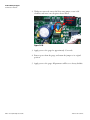
Source Housing Check................................................................... 10-2
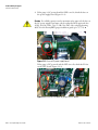
Replacing System PCBs..................................................................... 10-2
Chapter 11
Troubleshooting & Support........................................................................... 11-1
General Troubleshooting .................................................................. 11-1
The Detector-Transmitter................................................................. 11-3
The Current Output ......................................................................... 11-7
The Relay.......................................................................................... 11-7
Communication Problems ................................................................ 11-7
Contact Information ......................................................................... 11-9
Warranty........................................................................................... 11-9
Appendix A
Ordering Information....................................................................................... A-1
Appendix B
Specifications................................................................................................... B-1
DensityPRO Gauge User Guide
ix
Contents
Appendix C
Solution Characterization............................................................................... C-1
Overview............................................................................................ C-1
Defining a Solution Polynomial ......................................................... C-1
Built-In Polynomial Coefficients........................................................ C-2
Appendix D
Attenuation Coefficients .................................................................................D-1
Overview............................................................................................ D-1
Attenuation Coefficients .................................................................... D-1
Appendix E
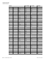
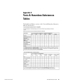
Toxic & Hazardous Substances Tables ....................................................... E-1
Appendix F
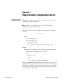
Vapor Density Compensated Level ................................................................F-1
Introduction........................................................................................ F-1
Finding a Compensation Formula....................................................... F-2
Special Equation ................................................................................. F-3
Gauge Setups ...................................................................................... F-4
Wiring ................................................................................................ F-5
Appendix G
Using the DensityPRO Gauge as a Point Level Gauge..............................G-1
Overview............................................................................................ G-1
Point Level Setup ............................................................................... G-1
Appendix H
X-ray Safeguard Software Setup ..................................................................H-1
Overview............................................................................................ H-1
Setup.................................................................................................. H-1
Index ..........................................................................................................INDEX-1
x
DensityPRO Gauge User Guide
Thermo Fisher Scientific
Safety Information & Guidelines
This section contains information that must be read and understood by all
persons installing, using, or maintaining this equipment.
Safety
Considerations
Failure to follow appropriate safety procedures or inappropriate use of the
equipment described in this manual can lead to equipment damage or
injury to personnel.
Any person working with or on the equipment described in this manual is
required to evaluate all functions and operations for potential safety hazards
before commencing work. Appropriate precautions must be taken as
necessary to prevent potential damage to equipment or injury to personnel.
The information in this manual is designed to aid personnel to correctly
and safely install, operate, and/or maintain the system described; however,
personnel are still responsible for considering all actions and procedures for
potential hazards or conditions that may not have been anticipated in the
written procedures. If a procedure cannot be performed safely, it must not
be performed until appropriate actions can be taken to ensure the safety
of the equipment and personnel. The procedures in this manual are not
designed to replace or supersede required or common sense safety practices.
All safety warnings listed in any documentation applicable to equipment
and parts used in or with the system described in this manual must be read
and understood prior to working on or with any part of the system.
Failure to correctly perform the instructions and procedures in this
manual or other documents pertaining to this system can result in
equipment malfunction, equipment damage, and/or injury to personnel.
Warnings,
arnings,
Cautions, &
Notes
The following admonitions are used throughout this manual to alert users
to potential hazards or important information. Failure to heed the
warnings and cautions in this manual can lead to injury or equipment
damage.
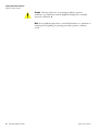
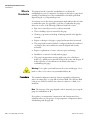
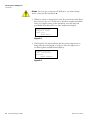
Warning Warnings notify users of procedures, practices, conditions, etc.
which may result in injury or death if not carefully observed or followed.
The triangular icon displayed with a warning may contain a lightning bolt
or the radiation symbol, depending on the type of hazard. ▲
Thermo Fisher Scientific
DensityPRO Gauge User Guide
xi
Safety Information & Guidelines
Warnings, Cautions, & Notes
Caution Cautions notify users of operating procedures, practices,
conditions, etc. which may result in equipment damage if not carefully
observed or followed. ▲
Note Notes emphasize important or essential information or a statement of
company policy regarding an operating procedure, practice, condition,
etc. ▲
xii
DensityPRO Gauge User Guide
Thermo Fisher Scientific
Chapter 1
Product Overview
Introduction
The Thermo Scientific DensityPRO gamma density system is designed to
provide reliable, accurate process material density measurements for a wide
variety of challenging applications. The gauge is mounted outside of the
process vessel and never contacts the process material. The gauge can
measure the density of almost any liquid, slurry, emulsion, or solution.
The gauge can convert the basic density measurement into a variety of
output measurements as appropriate for specific applications, e.g., bulk
density or solids content per unit volume. Given a temperature input, the
gauge can compensate the density measurement relative to a user-specified
reference temperature. If a flow input is provided, it can calculate mass
flow.
The system consists of the source head, which contains the radioisotope
source, and the integrated detector-transmitter, which contains the
scintillator detector and electronics. The radioisotope source emits gamma
radiation that passes through the process material. The detector measures
the energy of the radiation arriving at the detector after passing through the
process material (and vessel walls). The gauge determines the density of the
process material by measuring the amount of radiation arriving at the
detector, which varies with the density of the process material.
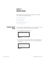
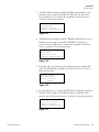
Note The gamma radiation used by the gauge cannot make the vessel,
process or structure radioactive. ▲
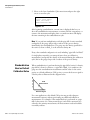
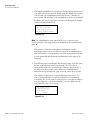
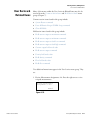
Figure 1–1.
Thermo Fisher Scientific
DensityPRO Gauge User Guide
1-1
Product Overview
Functional Description
The Source
A Cesium (Cs-137) radioisotope source is used for most applications. A
Cobalt (Co-60) source is available for applications requiring a higher
energy source. The radioisotope is bound in ceramic pellets and double
encapsulated in a pair of sealed stainless steel containers. The resulting
source capsule is highly resistant to vibration and mechanical shock.
The source capsule is further enclosed in the source head, a lead-filled,
welded steel housing. A shaped opening in the lead shielding directs the
gamma radiation beam through the process material towards the detector.
Outside of the beam path, the energy escaping the source head is very low
and well within prescribed limits.
Closing the source shutter allows the beam to be turned off (the shutter
blocks the radiation) during installation or servicing of the gauge. All
source housings meet or exceed the safety requirements of the U.S. Nuclear
Regulatory Commission (NRC) and Agreement State regulations. Refer to
the Gamma Radiation Safety Guide (p/n 717904).
The Integrated
DetectorTransmitter
The DensityPRO system uses a scintillator-type detector to measure the
radiation reaching the detector from the source. The detector consists of a
special plastic scintillator material and a photomultiplier tube with the
associated electronics. When radiation strikes the plastic scintillator
material, small flashes of light are emitted. As the density of the process
material increases, more gamma radiation is attenuated by the process
material and fewer light pulses are generated by the scintillator material.
The photomultiplier tube and associated detector electronics convert the
light pulses into electrical pulses that are processed to determine the process
material density and related measurement values.
Functional
Description
Measurement
Calculation
After the gauge calculates the process material density, it can convert the
measurement into a number of forms. For a slurry (solid material in a
carrier fluid), the gauge can provide measurements based on the ratio of
solids to carrier. Similar measurements can be made for emulsions (two
different fluids) and for solutions (a solute material dissolved in a solvent
fluid).
By inputting flow data, the DensityPRO gauge can generate mass flow
measurements. A 4–20 mA current output from a magnetic flow sensor or
from a fixed or portable flow meter can be input to the gauge.
For applications that require temperature compensation, the gauge can
accept a temperature input to compensate the density measurement for
changes in process temperature.
1-2
DensityPRO Gauge User Guide
Thermo Fisher Scientific
Product Overview
Functional Description
Communications &
Measurement
Display
Communication with the gauge can be via the RS485 or the RS232 serial
ports using a Thermo Scientific Model 9734 handheld terminal (HHT), a
PC with the Thermo Scientific TMT Comm communication software or
other terminal emulation software installed, or a standard ANSI or VT-100
terminal.
The HART communication protocol is supported over the 4–20 mA
current output with an optional daughter board. Communication with the
gauge is through the 275, 375, 475, or later field communicator from
Emerson Electric Co. Refer to the DensityPRO gauge with HART
operation guide (p/n 717817) for instructions.
With the FOUNDATION™ fieldbus communication option, the
DensityPRO system provides users with access to control or program
parameters via a host system.
Once the gauge has been set up, the primary (density) measurement is
displayed on the external display, if present, and on the remote terminal or
HHT.
Inputs & Outputs
The characteristics of the input and output options for the DensityPRO
system are summarized in the table below.
Table 1–1.
Thermo Fisher Scientific
Type
Characteristics
Comments
Current output
Three configurations available for
the 4–20 mA current output:
- Isolated, loop-powered (default)
- Non-isolated, self-powered
- Isolated, self-powered output
(requires optional daughter board
p/n 886595)
Default range is 4–20 mA DC.
One current output is provided
on the CPU board.
Serial
communications
RS485 half duplex
RS232 full duplex
Half duplex communication to
PC or HHT.
Full duplex communication with
remote terminal or PC.
HART
communications
HART protocol supported over the 4–
20 mA current output.
Optional daughter board
required.
FOUNDATION
fieldbus
communications
The Device Description is a DD4 that
is interpreted by a host
implementing DD Services 4.x or
higher.
The DD is available from the
Fieldbus Foundation website.
Optional relays
Two relays optionally available on
the AC power/ relay board.
Form C relays, SPDT, isolated 8 A @
220 Vac.
Process alarms and system
fault or warning alarms can be
assigned to control
(open/close) relays.
DensityPRO Gauge User Guide
1-3
Product Overview
Other Features
Type
Characteristics
Comments
Inputs
Flow meter: 4–20 mA linear
Dry contact closure
Temperature compensation circuitry
with 100-ohm Platinum RTD, 2 or 3
wire
Execute system commands
based on a user-provided
contact switch opening or
closing input.
Optional Thermo
Scientific Model
9723 display
Backlit LCD for measurement
readouts.
2-line x 16-character.
Up to four measurement
readouts can be displayed at a
time.
Other Features
In addition to the functionality discussed above, the DensityPRO system
has the following features.
Dynamic Menu
System
The setup menus enable you to quickly configure the gauge by requiring
you to enter all of the basic parameters. Additional menu groups contain
fields in which you can enter specialized parameters and commands,
allowing you to customize the gauge for a wide variety of applications.
Direct access codes are also provided, allowing experienced users to access
menu items and commands directly, bypassing the menu system.
Instantaneous
Response
Multiple Readouts
Process Alarms
1-4
DensityPRO Gauge User Guide
Thermo Fisher Scientific’s Dynamic Process Tracking (DPT) ensures there
is no lag time in the system response to significant changes in process level.
When changes occur, the DPT feature reduces the normal averaging time
constant by a factor of eight, ensuring a rapid, smooth output response.
When the process stabilizes, a longer time constant is applied to reduce the
fluctuations inherent in radiation-based measurements. In this way, process
level changes are immediately reflected in the transmitter output, while the
effects of statistical variations in the radiation measurement are greatly
reduced.
Select up to eight measurement values for display.
Define up to 16 process alarms in addition to the built-in system fault
alarms and warning alarms.
Thermo Fisher Scientific
Product Overview
Associated Documentation
Totalizers and Batch
Control
Output Signals
Associated
Documentation
Thermo Fisher Scientific
Four independent totalizers may be configured to “count” elapsed time or
cumulative mass / volume when a flow input signal is provided and a mass
/ volume-flow measurement has bee defined. Totalizers can be assigned to
drive relays. Relays can be set to open or close at specified “slow” or “stop”
counts for batch or sample control.
Any measurement can be assigned to the 4–20 mA current output, or the
measurement values can be sent to a remote terminal or host computer as
serial data. The two contact closure inputs can be used to activate any
system command based on a user-provided switch input (open or close).
Two relay outputs are available on the optional AC power / relay board.
Along with this guide, the following documents must be read and
understood by all persons installing, using, or maintaining this equipment:
●
DensityPRO gauge installation guide, p/n 717774
●
Gamma radiation safety guide, p/n 717904
●
DensityPRO gauge with FOUNDATION™ Fieldbus Application Guide,
p/n 717917 (if FOUNDATION fieldbus installed)
●
DensityPRO / DensityPRO+ gaugewith HART operation manual, p/n
717816 (if using HART protocol)
●
Model 9734 handheld terminal operation manual, p/n 717797 (if
using the Thermo Scientific handheld terminal)
DensityPRO Gauge User Guide
1-5
This page intentionally left blank.
Chapter 2
Getting Started
Warning In the United States, you may uncrate and mount the source
housing, but you may not remove the shipping bolt unless you are licensed
to commission the gauge. In Canada, you must have a license condition
permitting mounting / dismounting, and without this condition, users may
not remove the source from the shipping crate. ▲
Warning The DensityPRO system is a nuclear device regulated by federal
and / or state authorities. You are responsible for knowing and following
the pertinent safety and regulatory requirements. Refer to the Gamma
Radiation Safety Guide (p/n 717904). ▲
Communications
Setup
Serial
rial
Communications
This section assumes that the system has been properly installed and all
required connections have been made (reference the DensityPRO gauge
installation guide, p/n 717774).
The gauge provides one RS232 single-drop and on RS485 multi-drop serial
interface. An RJ-11 connector (phone jack) is also provided for the RS485
port.
The serial port on a personal computer (COM1, COM2, etc.) can be
connected directly to the gauge’s RS232 port. An RS485/RS232 adapter is
required to connect a PC to the gauge’s RS485 port. You can then
communicate with the gauge from a PC running TMT Comm software or
other terminal emulation software, such as HyperTerminal.
In non-hazardous locations the Thermo Scientific Model 9734 HHT can
be connected directly to the RJ-11 connector.
Note The HHT requires an 8 Vdc power source. The RJ-11 connector (6
wide, 4 conductor) for the RS485 port uses two wires (+Data, -Data) for
RS485 communications and two wires (+8 Vdc, common) for the 8 V
supply. ▲
Thermo Fisher Scientific
DensityPRO Gauge User Guide
2-1
Getting Started
Communications Setup
The default communication settings for the gauge RS232 and RS485 ports
and for the HHT are:
●
7 data bits
●
even parity
●
1 stop bit
●
9600 baud data rate
For additional information on setting up serial communications, refer to
“Serial Ports” (Chapter 8).
HART
Communication
Protocol
The HART communication protocol is supported over the 4–20 mA
current output and requires an optional daughter board. Communication
with the gauge is via the 275, 375, 475, or later field communicator from
Emerson Electric Co. As practical, the HART menu structure mirrors the
menu structure as described in this guide. Additional information can be
found in the DensityPRO / DensityPRO+ gauge with HART operation
guide (p/n 717816).
Once the optional HART board is installed, the instrument enters a special
mode of operation. In this mode, all user-entered RS232 selections are
overridden and the RS232 setup functions are disabled. The HART
interface provides access to basic setup functions, including primary
measurement setup, process alarms, additional measurements, current
output settings, gauge fine tuning, and action items.
Note Do not use the HART communication system for technical
troubleshooting. You must use either the Model 9734 or a computer with
RS232/RS485 converter and the TMT Comm software to access the
technical troubleshooting capabilities of the DensityPRO system. ▲
2-2
DensityPRO Gauge User Guide
Thermo Fisher Scientific
Getting Started
Gauge Operation
Gauge Operation
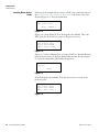
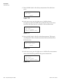
The first time you apply power to the instrument (after establishing
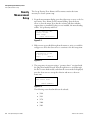
communication with the gauge), the message below is displayed. If the
display is blank, refer to Chapter 11 for troubleshooting procedures.
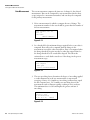
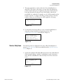
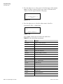
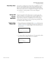
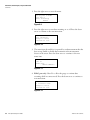
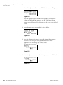
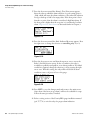
Unit has not
been set up!
For setup, press
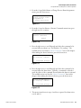
Figure 2–1.
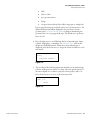
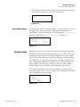
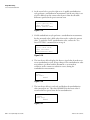
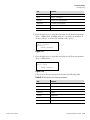
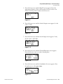
Once the gauge has been set up, the measurement display will show the
primary (density) measurement along with any additional measurements
that have been defined. An example of a density measurement readout is
illustrated below.
3.10 g/ml
For setup, press
Figure 2–2.
The measurement display is continuously updated except when the setup
menus are being accessed. The displayed measurement values are updated
approximately once every two seconds. Measurements are updated at a
much faster rate internally by the software. All measurements continue to
be updated even when they are not being displayed.
By default, the fourth line displays the “For setup” prompt or alarm /
warning messages when they occur. Up to six measurements can be
displayed (three at a time). Up to eight measurements can be displayed
(four at a time) by disabling the “For setup” prompt. See “Special
Functions” (Chapter 8) for instructions.
Thermo Fisher Scientific
DensityPRO Gauge User Guide
2-3
Getting Started
Gauge Operation
Entering Data
The keys used to operate the instrument are described in the table below.
Note A “Bad entry values” message is displayed if you enter values that the
gauge cannot understand. If this happens, the gauge will display the bad
entry information when you enter the setup menus. ▲
Table 2–1.
The Setup Menus
Key
Action
Right arrow
Press to enter the setup menus and to step through the top-level
menu headings. Also use to scroll through the list of menu options.
Up arrow
Return to the previous menu item or scroll through menu items in
the reverse direction.
Left arrow
Press to return to the previous option.
Down arrow
Press to select an option and continue to the next menu item.
Decimal
Press once to enter a decimal. Press twice to enter the decimal in
scientific notation. For example, to enter 4.567E6, press 4.567.6
If you are entering data from a terminal keyboard, you can press E or
e before entering the exponent value rather than pressing the
decimal key twice.
Number keys
Press to enter data values. Press the down arrow to indicate the end
of the number entry.
Minus sign
Press to indicate a negative number.
The setup menus take you through the steps for entering the data required
for instrument operation. In each menu item, data values that can be
entered or changed are flashing. Enter the requested parameter in each
menu item as it is displayed to ensure other related menu items are
displayed. For example, to set up an alarm, you must enter a value for the
set point menu item in order to activate the rest of the Alarm Setup menu.
To exit the setup menus, press the EXIT key on the HHT or press x on the
terminal keypad. This will save any changes you made and return you to
the measurement display.
Note When accessing the setup menus, the display times out and returns
to the measurement display if no entries are made for five minutes.
Changes or entries made up to that point are saved and used by the
instrument. ▲
2-4
DensityPRO Gauge User Guide
Thermo Fisher Scientific
Getting Started
Gauge Operation
Note The appearance of many menu items varies dynamically with context
and depends on the parameter values and selections entered during setup.
Thus, the appearance of the menu items as described in this manual may
vary slightly from what is actually displayed on the gauge. ▲
Reset to Factory Defaults
If the display shown in Figure 2–1 is not displayed upon power-up, the
instrument has been at least partially set up. If you do not want the
instrument to use these settings or if the instrument has been moved to a
new location, you can restore factory defaults.
Use command DAC 82 (Erase All Entries Except COMM Setup) to reset
all user entries except communication settings to factory defaults. Use
command DAC 74 (Erase All Entries) to reset all user entries including
communication settings to factory defaults.
Service Only Menu
Items
The menu structure has two “layers” of menu items, the user layer and the
service layer. The user layer is adequate for most applications, while the
service layer provides a number of additional, special purpose menu items.
These additional tools (service only items) can be enabled using the Special
Functions menu (Chapter 8).
Thee Direct Access
Method
The direct access method allows users to bypass the menu structure and
directly access a specific menu item. Note that most menu items display a
slightly different message when accessed using this method. In order to use
this method, you must know the direct access code (DAC or keypad code).
Parameter DACs have six digits, and command DACs have one, two, or
three digits.
To find the DAC for a particular menu item:
1. Scroll to the desired menu item.
2. If the menu item is not for a floating point number entry (an entry
containing a decimal point), press the decimal key to display the DAC
information screen. If the menu item is for floating point entries, press
decimal followed by up arrow to display the DAC information screen.
Caution Use the direct access method with caution. When entering or
changing a parameter value for one menu item, you may also need to enter
or modify the value of other menu items. ▲
Thermo Fisher Scientific
DensityPRO Gauge User Guide
2-5
Getting Started
Gauge Operation
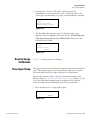
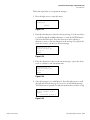
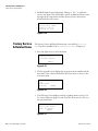
Locating Direct Access
Codes
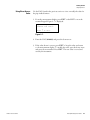
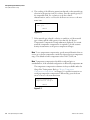
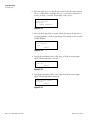
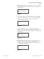
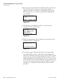
Following is an example of how to locate a DAC. One of the first items in
the Set up Density, Den. Alarms, & Flow menu is the Sensor Uses item,
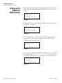
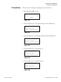
shown in Figure 2–3. Press the decimal key.
Sensor uses
5202 source head
NEXT↓
CHANGE
Figure 2–3.
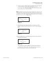
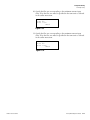
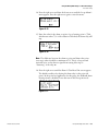
Figure 2–4 is then displayed. Note the keypad code: 005002. This is the
DAC. Press the down arrow to return to the previous screen.
Value is 6
Item is data entry
Keypad code 005002
{HEX = 050C} Press ↓
Figure 2–4.
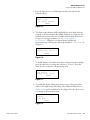
Figures 2–5 and 2–6 illustrate how to locate a DAC for a decimal (floating
point) data entry item. At the Pipe Inside Diameter item shown in Figure
2–5, press the decimal key followed by the up arrow.
Pipe inside diameter
4.000 in
NEXT↓
Figure 2–5.
Note the keypad code (048003). Press the down arrow to return to the
previous screen.
Value is 4.000
Item is data entry
keypad code 048003
{HEX = 300F} Press
Figure 2–6.
2-6
DensityPRO Gauge User Guide
Thermo Fisher Scientific
Getting Started
Gauge Operation
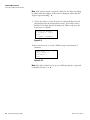
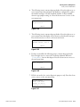
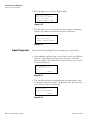
Using Direct Access
Codes
Use the DAC found in the previous section to view or modify the value for
the pipe inside diameter:
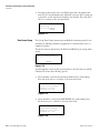
1. From the measurement display, press EXIT on the HHT or x on the
terminal keypad. Figure 2–7 is displayed.
Key in entry ID or
command code then
Press to exit.
Figure 2–7.
2. Enter the DAC (048003) and press the down arrow.
3. If the value shown is correct, press EXIT to keep the value and return
to the measurement display. To modify the value, press the down arrow
and enter the new number. Press EXIT. The new value is stored and
used by the instrument.
Thermo Fisher Scientific
DensityPRO Gauge User Guide
2-7
This page intentionally left blank.
Chapter 3
Set up Density, Den. Alarms, & Flow
Overview
Thermo Fisher Scientific
The Set up Density, Den. Alarms, & Flow menu takes you through the
steps required for basic system setup:
●
Specify the source head model.
●
Select the material type that best defines your process material.
●
Set up temperature compensation (if required).
●
Select the primary measurement and units.
●
Enter the values of the primary measurement that correspond to the
maximum and minimum values of the current output.
●
Set the decimal point position for the primary measurement readout.
●
Set up a process alarm for the primary measurement.
●
Select the flow input settings (if any) to be used. (The flow input source
must be defined before a flow related measurement readout can be
configured.)
●
Perform a standardization measurement that provides the gauge with a
standard configuration reference point.
●
Perform calibration measurement(s), if necessary, to fine tune the gauge
for the process material.
DensityPRO Gauge User Guide
3-1
Set up Density, Den. Alarms, & Flow
Density Measurement Setup
Density
Measurement
Setup
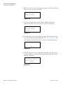
The Set up Density, Den. Alarms, & Flow menu contains the items
necessary for a basic system setup.
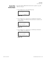
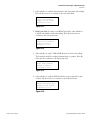
1. From the measurement display, press the right arrow to move to the Set
up Density, Den. Alarms, & Flow menu heading. Press the down
arrow to enter the menu. Note that the software will detect whether
output relays are installed. If relays are not installed, the menu heading
will be “Set up Density and Flow.”
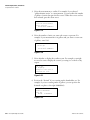
Set up density, den.
alarms & flow
Exit setup.
Other functions
Figure 3–1.
2. Help screens are provided throughout the menus to assist you with the
setup process. Press the down arrow to continue to the first setup item.
General HELP text.
{Information on how
to set up this
gauge}
NEXT
Figure 3–2.
3. The gauge tunes its response using a “geometry factor” associated with
the gauge head model selected. Press the right arrow to scroll through
the list of source head models, and when the correct model is displayed,
press the down arrow to accept the selection and move to the next
menu item.
Sensor uses
5202 source head
NEXT CHANGE
Figure 3–3.
The following source head models can be selected:
3-2
DensityPRO Gauge User Guide
●
5190
●
5191
●
5176
●
5200
●
5201
Thermo Fisher Scientific
Set up Density, Den. Alarms, & Flow
Density Measurement Setup
●
5202
●
5203 or 5204
●
user’s geometry factor
●
Z-pipe
●
one-piece insertion head (also called a sugar pan or tank probe)
If your gauge head type is not listed, select “user’s geometry factor.” An
additional menu item will be displayed to let you enter a custom
geometry factor. Contact Thermo Fisher for help in determining the
geometry factor for your gauge head type. The default user’s geometry
factor is 0.85.
4. Press the right arrow to scroll through the list of material types: slurry,
solution, single phase, or emulsion. See “Material Type” later in this
chapter for detailed discussion. When the correct material type is
displayed, press the down arrow to accept the selection and move to the
next menu.
Material type is
slurry
CONTINUE CHANGE
Figure 3–4.
5. The wording of the following menu item depends on the material type
selection in the previous item. For a slurry, enter the specific gravity of
the carrier liquid. For a solution, enter the solvent gravity, and so on.
Press the down arrow to move to the next menu item.
Carrier gravity
.9982 g/cc
NEXT
Figure 3–5.
Thermo Fisher Scientific
DensityPRO Gauge User Guide
3-3
Set up Density, Den. Alarms, & Flow
Density Measurement Setup
6. The wording of the following menu item depends on the material type
selection in the previous item. For a slurry, enter the specific gravity of
the suspended solids. For a solution, set up the solution
characterization, and so on. Press the down arrow to move to the next
menu item.
Solids gravity
3.000 g/cc
NEXT
Figure 3–6.
7. If the material type selected is solution or emulsion or if the material
type is slurry and the solids gravity is less than 2.0, the Process
Temperature Compensation Setup submenu is displayed. For certain
materials, temperature compensation is required to provide accurate
density measurements as the process temperature changes.
Note To use temperature compensation, specify material densities that are
correct at a reference temperature outside the expected process temperature
range. The default reference temperature value is 20°C (68°F). ▲
Note Temperature compensation should be configured prior to
standardization, if the standard configuration is affected by temperature. ▲
The temperature compensation submenu is always available under the
Gauge Fine Tuning menu. Refer to “Process Temperature
Compensation Setup Menu” in Chapter 5 for specific instructions on
setting up temperature compensation. When ready, press the down
arrow to move to the next menu item.
Process temperature
compensation setup
NEXT
Figure 3–7.
3-4
DensityPRO Gauge User Guide
Thermo Fisher Scientific
Set up Density, Den. Alarms, & Flow
Density Measurement Setup
8. At the next screen, select the primary Available measurements depend
on the material type selected. This is discussed in “Primary
Measurement Type” later in this chapter. Press the down arrow when
you are ready to move to the next menu.
Note By default, the primary measurement is displayed as readout #1 and
is assigned to the current output signal. The primary measurement cannot
involve mass or flow. Mass or flow related measurements must be assigned
as additional measurements (Chapter 4). ▲
Primary measurement:
density
To change, press
NEXT
Figure 3–8.
9. Select the units system using the right arrow. Options are: ALL,
English, or Metric. Press the down arrow to move to the next menu
item.
Allow display of All
units. Change to:
Metric or English
NEXT
Figure 3–9.
10. Press the right arrow to scroll through and select the desired units for
the primary measurement.
Density
units = g/ml
To change, press
NEXT
Figure 3–10.
The complete list of units available for the density measurement is
provided in the following table. After making the desired selection,
press the down arrow to move to the next menu item.
Thermo Fisher Scientific
DensityPRO Gauge User Guide
3-5
Set up Density, Den. Alarms, & Flow
Density Measurement Setup
Table 3–1. Units for the density measurement
Abbreviation
Unit
g/ml
grams per milliliter
lb/US gal
pounds per US liquid gallon
lb/UK gal
pounds per UK or imperial gallon
lb/cu ft
pounds per cubic foot
ston/cu yd
short tons (2,000 lb) per cubic yard
lton/cu yd
long tons (2,240 lb) per cubic yard
g/l
grams per liter
oz/cu in
ounces per cubic inch
lb/cu in
pounds per cubic inch
g/cu in
grams per cubic inch
lb/cu yd
pounds per cubic yard
deg API
degrees, American Petroleum Institute
deg Be (L)
degrees, Baumé, light scale
deg Be (H)
degrees, Baumé, heavy scale
deg Tw
degrees, Twaddle
11. Press the right arrow to scroll through and select the units that will be
used to specify the pipe inside diameter. The available units depend on
the selection made earlier in the Allow Display of menu item. Press the
down arrow to continue to the next menu item.
Size units = in
To change to ft, yd,
M, cm, or mm press
NEXT
Figure 3–11.
12. Enter the value for the pipe inside diameter in the units selected in the
previous menu item. Press the down arrow to continue.
Pipe inside diameter
4.000 in
NEXT
Figure 3–12.
3-6
DensityPRO Gauge User Guide
Thermo Fisher Scientific
Set up Density, Den. Alarms, & Flow
Density Measurement Setup
13. Set the measurement range for the current output.
Meas #1 is associated with the density measurement, and the current
output value is associated with Meas #1 by default.
Note The range for the primary measurement value specified for the
current output does not affect the range of the measurement values that are
displayed. ▲
Enter the density value at which the current output will be at
maximum. The default maximum current output value is 20 mA. Then
press the down arrow.
Meas #1 reading for
20.00 mA output:
3.000 g/ml
NEXT
Figure 3–13.
Enter the density value at which the current output will be at
minimum. The default minimum current output value is 4 mA.
Meas #1 reading for
4.000 mA output:
2.000 g/ml
NEXT
Figure 3–14.
The operational range for current output can be set anywhere within
the range from 3.8 to 20.5 mA. The default range for the current
output is 4 to 20 mA. The Fault Low and Fault High current output
levels are 3.6 mA or lower and 20.8 mA or greater, respectively. See
“Modify or Reassign Current Output” (Chapter 6) for details on
modifying the current output range.
Display Scaling
Specifying a value greater than 9,999 for the maximum current output
reading enables the Display Scaling menu items. For example, values in
the range from 0 to 100,000 can be scaled by a factor of 100 to a range
of 0 to 1,000 so that the displayed values do not exceed the limits of
the four-digit numerical display. See “Display Scaling” (Chapter 4).
Thermo Fisher Scientific
DensityPRO Gauge User Guide
3-7
Set up Density, Den. Alarms, & Flow
Density Measurement Setup
14. Use the right or left arrow to adjust the position of the decimal point
for the Meas #1 readout. A maximum of three decimal places can be
displayed. Note that the decimal point position only affects how the
measurement value is displayed. It has no effect on the precision of the
internal value of the measurement computed by the gauge. When the
decimal position is set, press the down arrow to move to the next menu
item.
Position of decimal
in readout 1
000.0
{g/ml}
NEXT
CHANGE
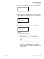
Figure 3–15.
15. Press the right arrow to enter the Set up Alarm 1 submenu and specify
process alarm #1 for the primary measurement. After defining alarm
#1, the submenu for alarm #2 will be displayed. Refer to “Alarm Setup”
later in this chapter.
Set up alarm 1
(Alarm point, etc.)
NEXT
Figure 3–16.
16. Press the right arrow to enter the Flow Input Setup submenu. The
gauge can accept a 4 –20 mA current input signal from an external flow
meter. This menu prompts you for the parameters required to set up
the flow input and the units for volume and mass flow measurements.
This menu is also available under the Gauge Fine Tuning menu chain.
See “Flow Input Setup” (Chapter 5) for detailed information.
Flow INPUT setup
NEXT
Figure 3–17.
17. After the Flow Input Setup menu, menu items related to gauge
standardization and calibration are displayed. These items are discussed
later in this chapter.
3-8
DensityPRO Gauge User Guide
Thermo Fisher Scientific
Set up Density, Den. Alarms, & Flow
Density Measurement Setup
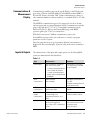
Material Type
Use the Material Type menu item to select the material type that best
matches your process material, slurry, solution, single phase, or emulsion.
Note If you only want to measure the overall density of the process
material, you can select single phase as the material type regardless of the
material’s makeup. ▲
The basic setup does not include gamma ray attenuation coefficients. The
default settings are usually adequate, however, you should change
attenuation coefficients if your source is not Cs-137 or in other special
situations. See “Attenuation Coefficients” (Appendix D).
After a material type is selected, additional menu items are displayed so that
required specific gravity values for that material type can be entered. These
additional menu items are discussed below.
Slurry
If the material type selection is slurry, menu items will prompt you for the
following values.
Carrier gravity: Enter the specific gravity of the carrier liquid in g/cc.
The default value is 0.9982, correct for water at sea level and 20°C
(68°F).
Solids gravity: Enter the dry, solid density of your suspended solids in
g/cc. The default is 3.0 g/cc. For example, a 1 cc block of solid basalt
has about 3.0 grams of mass.
Solution
If the material type selection is solution, menu items will prompt you for
the following values.
Solvent gravity: Enter the specific gravity of your solvent liquid in g/cc.
The default value is 0.9982, correct for water at 20°C (68°F).
Solution characterization: Solution characterization is a setting that
relates the solution’s density to its concentration using a polynomial
formula. You can select one of several aqueous solutions for which the
gauge has built-in polynomials. Each built-in solution is listed with the
concentration range over which the setting can be used. For example, if
you select “D-Fructose 0-60%,” the gauge can measure fructose
concentrations up to 60 percent in water. If your solution is not listed
in the menu, see “Solution Characterization” (Appendix C) for
information about entering a user-defined solution characterization
polynomial or break point table.
Thermo Fisher Scientific
DensityPRO Gauge User Guide
3-9
Set up Density, Den. Alarms, & Flow
Density Measurement Setup
Single Phase
Emulsion
If the mixture in the pipe has multiple changing variables, the process
material must be treated as one product in order to give an average density.
In this case, select single phase.
If the material type selection is emulsion, menu items will prompt you for
the following values.
Fluid_1 gravity: Enter the specific gravity of your carrier liquid in g/cc.
The default value is 0.9982, correct for water at 20°C (68°F).
Fluid_2 gravity: Enter the specific gravity of your suspended liquid in
g/cc. For example, 0.88 is a typical specific gravity for petroleum. The
default is 3 g/cc.
Primary
Measurement Type
From the Primary Measurement Type screen, select from the
measurements listed below as appropriate for the material type.
●
Density: The ratio of mass to volume. For example, a material has a
density of 500 g/l if 1 liter of the material weighs 500 grams on a
balance scale.
●
Bulk Density: If the material type is solution or single phase and
temperature compensation is being used, the density value is
compensated for temperature and the value displayed is the density as it
would be at the reference temperature. In this case, select bulk density
to measure and display the uncompensated density of the material at
the process temperature.
●
If material type is slurry:
Solids content/vol: The concentration, or mass of solids suspended
in a volume of slurry. For example, the slurry has a solids
concentration of 270 g/l if one liter of slurry contains 270 grams of
suspended solids.
Carrier content/vol: The concentration, or mass of carrier in a
volume of slurry. For example, the slurry has a carrier concentration
of 910 g/l if 1 liter of slurry contains 910 grams of carrier liquid.
Solids/carrier: The ratio of suspended solids mass to the volume of
the carrier liquid. For example, the slurry has a solids to carrier ratio
of 2 lb/gal if 2 pounds of solids are mixed with every 1 gallon of
carrier. (In some applications, this measurement is called pounds of
sand added because it measures the mass of solids added to a
volume of carrier. This differs from solids concentration, which
measures the mass contained in a volume of slurry.)
3-10
DensityPRO Gauge User Guide
Thermo Fisher Scientific
Set up Density, Den. Alarms, & Flow
Density Measurement Setup
Percent by weight solids (carrier): The percentage of a component
that makes up the process material’s mass. For example, the slurry is
30% by weight solids if each kilogram of material contains 300
grams of suspended solids.
Percent by volume solids (carrier): The percentage of a component
that makes up the process material’s volume. For example, the
slurry is 80% by volume liquid if each liter of material contains 800
milliliters of liquid carrier.
●
If material type is solution:
Solute content/vol: The concentration or mass of solute dissolved
in a volume of solution. Similar to solids content/vol for slurries.
Solvent content/vol: The concentration or mass of solvent in a
volume of solution. Similar to carrier content/vol for slurries.
Solute/solvent: Similar to the solids to carrier ratio for slurries.
Percent by weight solvent (solute): Similar to percent by weight
solids (carrier) for slurries.
Percent by volume solvent (solute): Similar to percent by volume
solids (carrier) for slurries.
●
If material type is emulsion:
Fluid_2 content/vol: The concentration or mass of fluid_2
suspended in a volume of emulsion. Similar to solids content/vol
for slurries.
Fluid_1 content/vol: The concentration or mass of fluid_1 in a
volume of emulsion. Similar to carrier content/vol for slurries.
Fluid_2/Fluid_1: Similar to the solids to carrier ratio for slurries.
Percent by weight Fluid_2 (Fluid_1): Similar to percent by weight
solids (carrier).
Percent by volume Fluid_2 (Fluid_1): Similar to percent by volume
solids (carrier).
Note The gauge will be calibrated in terms of the primary measurement.
The calibration will be more accurate if you select a primary measurement
that can be accurately verified by measuring samples. ▲
Thermo Fisher Scientific
DensityPRO Gauge User Guide
3-11
Set up Density, Den. Alarms, & Flow
Alarm Setup
Alarm Setup
The Set up Alarm 1 submenu appears after the density measurement items.
Enter this submenu to set up an alarm.
Set up alarm 1
(Alarm point, etc.)
NEXT
Figure 3–18.
This subgroup allows you to assign and set up a process alarm for the
density measurement. You can define up to 16 process alarms. It is
recommended that you keep a record of each alarm set up (assigned
measurement, set point, clear point, alarm action) for future reference.
By default, all process alarms are assigned to Meas #1 (the primary
measurement). You can assign process alarms for any additional
measurements that have been set up. The procedure is the same as the
procedure detailed below.
1. From the Set up Alarm 1 screen, press the right arrow to access the
menu items.
2. Enter the process density at which the alarm will activate. Note that the
screen below is an example only. Alarm 1 can be set as either a high
density alarm or low density alarm. Press the down arrow to continue.
Exit alarm 1 setup
Alarm 1 set point
2.000 g/ml
NEXT HELP
Figure 3–19.
Note A set point must be entered to activate the remaining menus in this
subgroup. ▲
3-12
DensityPRO Gauge User Guide
Thermo Fisher Scientific
Set up Density, Den. Alarms, & Flow
Alarm Setup
3. Select a clear point or dead band to clear the alarm. Press the down
arrow to continue to the next screen.
Alarm 1 clear based
on clr point
Chng to “dead band”
Continue as is.
Figure 3–20.
Set Point and Clear Point / Dead Band
An alarm is defined with a set point / clear point configuration or a set
point / dead band configuration. The set point defines the
measurement value at which the alarm is activated. The clear point or
dead band defines the measurement value at which the alarm is cleared
(alarm ceases).
A clear point sets a fixed measurement value at which the alarm clears.
The value of the clear point is independent of the set point and remains
the same even if the set point is moved.
A dead band defines a fixed distance between the set point and an
implicit clear point. If the set point is moved, the implicit clear point
moves also, maintaining the distance from the set point specified by the
dead band. For example, if a set point is defined at 2.5 g/ml and the
dead band is set at 1.0 g/ml, the implicit clear point will be at 3.5 g/ml.
Changing the set point from 2.5 g/ml to 3.0 g/ml move the implied
clear point from 3.5 g/ml to 4.5 g/ml. The relative distance between
the implied clear point and the set point remains fixed at 1.0 g/ml, the
dead band value.
Use a clear point configuration if you want to be able to change the
alarm set point in the future without affecting the alarm clear point.
Use a dead band configuration if you want the alarm clear point to
remain at a fixed distance relative to the set point.
4. Enter desired clear point value. The clear point is the process density
where you want the alarm to stop alarming. If dead band was selected
above, enter the span of the dead band relative to the set point.
Alarm 1 clear point
2.500 g/ml
{Makes alarm “Low”
limit}
NEXT HELP
Figure 3–21.
Thermo Fisher Scientific
DensityPRO Gauge User Guide
3-13
Set up Density, Den. Alarms, & Flow
Alarm Setup
High Limit & Low Limit Alarms
An alarm is activated when the measurement value reaches the specified
set point. The relative values assigned to the set point and clear point
determine whether the alarm is a low limit alarm or a high limit alarm.
If the set point value is less than the clear point value (or if the dead
band value is positive), the alarm is a low limit alarm. In this case, the
alarm is activated as the measurement value decreases below the set
point value. The alarm stays active until the measurement value again
increases above the clear point value.
Similarly, if the set point value is greater than the clear point (or the
dead band value is negative), the alarm is a high limit alarm. In this
case, the alarm is activated when the measurement value increases
beyond the set point value. The alarm stays active until the
measurement value again decreases below the clear point value.
5. Use the right arrow key to cycle through actions that can be used to
indicate the alarm has been triggered. The default action is “Nothing”.
Other actions are described below. Once the desired selection is made,
press the down arrow to continue to the next menu item.
Alarm 1: g/ml
is indicated by
controlling relay 1
NEXT CHANGE
Figure 3–22.
3-14
DensityPRO Gauge User Guide
●
Controlling relay 1 (2): If relays are installed, assign relay 1 or 2
as the alarm indicator.
●
Zero output 1: Hold current output at zero while the alarm is
active.
●
Max output 1: Hold current output at maximum value while
the alarm is active.
●
Outputs to alt: Switch current output(s) to alternate mode if
alternate mode has been defined.
●
#1 act on ALM action: Executes the command pair assigned as
the #1action when the alarm is activated / cleared. This
selection is only displayed if an alarm action has been assigned.
The selection is repeated for #2 and #3 actions, if assigned.
Thermo Fisher Scientific
Set up Density, Den. Alarms, & Flow
Standardization
6. The following menu item is displayed if controlling relay 1 (or 2) was
selected in the previous menu item. By default, relays are turned on
when an alarm is activated and turned off when the alarm clears. Press
the right arrow to change to off and reverse this behavior.
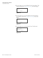
This is the final menu item in the Set up Alarm 1 menu group. Press
the left arrow to exit.
Relay 1 turns on
when alarm occurs.
Change to “off”
Exit alarm 1 setup.
Figure 3–23.
7. After you set up an alarm, the menu to set up the next alarm will be
displayed. Press the right arrow to set up the next alarm, or press the
down arrow to go on to the next menu item.
Set up alarm 2
(Alarm point, etc.)
NEXT
Figure 3–24.
Standardization
The standardization process takes a radiation measurement for a standard
process configuration to establish a reference point for the gauge. During
the standardization cycle, the gauge averages the detector signal. The
default cycle time lasts about 17 minutes. This averaged detector signal
provides a very repeatable measurement of the signal produced in the
standard configuration.
Once the standardization measurement has been completed, it can be
repeated at a later time to compensate for any changes, such as increased
attenuation due to process material buildup on the pipe walls. The gauge
can then adjust the calibration value(s) based on the new standardization
value. It is not necessary to repeat the calibration measurements, since the
calibration values are stored as a ratio of the calibration-to-standardization
measurement values. The calibration values are adjusted automatically
whenever a new standardization is performed.
Thermo Fisher Scientific
DensityPRO Gauge User Guide
3-15
Set up Density, Den. Alarms, & Flow
Standardization
When to
Standardize
The primary benefit of periodic standardization is it adjusts the
standardization point to compensate for changes in the tank or gauge head
assembly. Determining how often standardization should be performed
depends largely on your particular process.
A consistent error in the density measurement might indicate that it is time
to standardize again. It is generally a good idea to standardize the gauge
when one or more of the following conditions listed below occur.
●
Pipe wear is caused by corrosive or abrasive materials.
●
There is buildup of process material in the pipe.
●
Cleaning or spontaneous breakup of built-up material in the pipe has
occurred.
●
Repairs or changes to the pipe or gauge head mount have been made.
●
The gauge head mount has shifted or realigned, whether by accident or
on purpose (the source and detector must be aligned and securely
mounted).
●
Repair or replacement of source or detector parts and wiring.
●
Installation or removal of nearby nuclear gauges.
●
The gauge’s measurement accuracy might seem to be off if there is
debris (e.g., spilled process material) between the source and the pipe. If
debris is present, you should remove the debris rather than restandardizing the gauge.
Warning Do not place your hand between the source and the pipe. Use a
brush or other tool to remove any accumulated debris. ▲
Procedure
rocedure
The standard configuration must be a known repeatable configuration,
such as an empty pipe, or a pipe full of reference fluid. The reference fluid
is the process carrier for slurries, the solvent for solutions, or fluid_1 for
emulsions.
Note The accuracy of the gauge depends on how accurately you set up the
gauge for standardization. ▲
If you plan to use temperature compensation and if temperature has a
significant effect on your process, set up temperature compensation before
standardizing with the pipe full.
3-16
DensityPRO Gauge User Guide
Thermo Fisher Scientific
Set up Density, Den. Alarms, & Flow
Standardization
To perform the standardization cycle:
1. Put the gauge head and pipe in one of the following standard
configurations. Use the same standard configuration every time you
standardize.
a. Pipe full of carrier / solvent / fluid_1 / ref fluid: Fill the pipe with
pure carrier for slurries, pure solvent for solutions, or pure
“fluid_1” for emulsions. For single phase processes, you might need
to use a reference fluid that is completely different from the process
material.
b. Pipe empty: Standardizing on an empty pipe is suitable for some
applications when using small to medium pipes.
c. Full with block: Some installations come with a density reference
block to be placed in the beam path during standardization. Use
the block with a pipe full of reference fluid (such as pure carrier) if
so directed.
d. Empty with block: This configuration is similar to “full with
block.” Use it if you have a reference block and are directed to use
it with an empty pipe.
Note There is a selection called “Defer Standardization.” Do not make this
selection. ▲
2. Turn on (open) the source shutter.
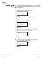
3. Enter the Sensor Head Standardization menu.
Sensor head
Standardization
NEXT
Figure 3–25.
4. Verify that the Standardize On menu item is set to the correct standard
configuration, as described in step 1.
Standardize on: pipe
full of carrier
To change, press
NEXT
Figure 3–26.
Thermo Fisher Scientific
DensityPRO Gauge User Guide
3-17
Set up Density, Den. Alarms, & Flow
Standardization
5. Move to the Start Standardize Cycle menu item and press the right
arrow to start the cycle.
Start standardize
cycle (tank empty)
Exit this menu.
NEXT EXECUTE CMD
Figure 3–27.
After beginning standardization, a menu item is displayed that lets you
abort the standardization measurement, continue with the setup menus, or
return to the measurement display where a countdown timer will display
the time remaining in the standardization cycle.
Note If you perform standardization with the pipe full of carrier standard
configuration, the gauge will provide a readout of the process density
immediately after standardization. The gauge uses the density specified for
the carrier (solvent or fluid_1) as the reference density. ▲
If any other standard configuration is used, including “pipe full of ref fluid”
for single phase materials, you must perform at least one calibration
measurement (and specify the density of the material during the calibration
cycle) before the gauge can provide a readout of the process density.
Standardization
Used as Default
Calibration Value
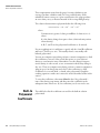
When standardization is performed using the pipe full of carrier for slurries,
pipe full of solvent for solutions, or pipe full of fluid_1 for emulsions, the
gauge uses the standardization measurement and the value for the carrier
gravity as a default calibration (CAL) point to convert the detector signal to
a density value as illustrated in the diagram below.
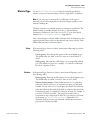
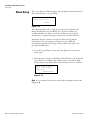
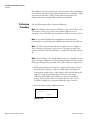
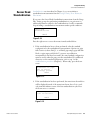
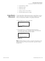
D
e
n
s
I
t
y
STD
Measurement
Detector Signal
For some applications, this default CAL point may provide adequate
measurement accuracy without performing any additional calibration
measurements. For example, if the standardization is performed on a pipe
full of clean carrier (for a slurry material type) and solids concentration is
selected as the primary measurement, the measurement readout should be
reasonably accurate.
3-18
DensityPRO Gauge User Guide
Thermo Fisher Scientific
Set up Density, Den. Alarms, & Flow
Calibration
Note Even if the gauge does not require calibration, it may be necessary to
perform periodic standardization. ▲
Calibration
Unless standardization is performed using the pipe full of carrier / solvent /
fluid_1 /ref fluid standard configuration, you must perform a calibration
measurement using the Density Gauge Calibration menus under the set up
menus.
If a calibration measurement is required, the message “Unit has not been
calibrated!” will be displayed. Even if calibration is not required, the default
calibration based on the standardization value may not provide sufficient
accuracy.
When calibration is required, a one-point (single point) calibration
measurement will be adequate for many applications. The calibration
measurement should be performed on actual process material with a
density near the nominal process density expected during normal
operation. In general, it is necessary to take samples of the process material
to determine the process density at the time of the calibration
measurement.
A one-point calibration provides a reference measurement at one density in
the range of interest. The gauge is able to measure other density values by
calculating the change in density corresponding to the change in the
detector signal using information about the source head (geometry factor),
the pipe dimension, and the process material.
If greater measurement accuracy is required, a two-point calibration
measurement can be performed. The second calibration measurement
applies a “slope” correction factor to the calculation used by the gauge to
convert the detector signal to the material density.
When using a two-point calibration, try to perform the first point
calibration on process material with a density near one end (high or low) of
the operational density range. Then perform the second calibration
measurement on process material with a density near the opposite end of
the range.
Note If the difference between the process densities at the calibration
points is too small, the measurement accuracy can actually be degraded by
the second CAL measurement rather than improved. ▲
Note If temperature compensation is active when you calibrate on a
solution or single phase material, determine the density of the process
sample(s) at the reference temperature. ▲
Thermo Fisher Scientific
DensityPRO Gauge User Guide
3-19
Set up Density, Den. Alarms, & Flow
Calibration
The calibration density value must be entered in terms of the measurement
type and units selected for the primary measurement. For example, if solids
concentration with units of lb/gal is the primary measurement, the
calibration density is actually solids concentration in lb/gal.
Calibration
Procedure
Use the following procedure to perform calibration.
Note The calibration measurement will replace any previous CAL 1 point.
The accuracy of the gauge’s density measurement depends on how
accurately you can determine the actual density of the process material. ▲
Note It is recommended that the standardization measurement be
performed prior to performing the calibration measurement if possible. ▲
Note The CAL 2 measurement and density value are used to calculate a
slope correction for the gauge response curve. The gauge uses this slope
correction and the CAL 1 measurement to compute the final density value.
▲
Note The procedure for the second calibration point is essentially the same
as for a one-point calibration. Go through the procedure below for the first
CAL point and repeat the procedure if a second CAL point is required. ▲
1. Fill the pipe with process material at a density in the range of interest.
Keep the process density as stable as possible during the calibration
measurement, and be ready to take samples of the material during the
calibration cycle. If performing this procedure for the second
calibration point, fill the pipe with process material of a different
density. It can be either more or less dense than for CAL 1, but it
should be as different as is practical within the range of interest.
2. Enter the Density Gauge Calibration menu.
Density gauge
calibration
NEXT
Figure 3–28.
3-20
DensityPRO Gauge User Guide
Thermo Fisher Scientific
Set up Density, Den. Alarms, & Flow
Calibration
3. Select a one or two-point calibration. If performing a two-point
calibration, try to perform the calibration measurements on process
densities near the low and high ends of the density range of interest.
Use 1 point CAL
Change to “2” point
Continue as is.
Figure 3–29.
4. Specify the number of time constant periods used for the calibration
measurement. The default CAL cycle is eight time constant periods. If
the default time constant (128 seconds) is used, calibration lasts about
17 minutes. If you decrease the CAL cycle time, the precision of the
calibration measurement is reduced. This can result in reduced
measurement accuracy. Setting the CAL cycle to less than two time
constants causes the cycle to abort automatically.
CAL cycle time:
8 x time constant
{time constant is
128 sec} NEXT HELP
Figure 3–30.
5. A non-zero value for the density must be entered before the rest of the
calibration menu items are displayed. If the exact density value is not
known at the time of the calibration, enter an approximate value, and
modify the value later.
CAL density
3.000 g/ml
NEXT HELP
Figure 3–31.
The “density” value entered for this menu item must be in terms of the
measurement type and units that has been selected for the primary
measurement (e.g., solids content/vol in kgram/liter).
Note If the CAL density value is changed after the command to use the
CAL value has been executed (see below), you must execute a CMD 6
(Process and Store) before the gauge will use the new CAL density value. ▲
Thermo Fisher Scientific
DensityPRO Gauge User Guide
3-21
Set up Density, Den. Alarms, & Flow
Calibration
6. If you have configured temperature compensation, the following menu
items will appear.
a. Process Temperature Learned: This item displays the process
temperature that was measured during the most recent CAL cycle.
This value is only displayed until the Use Latest CAL Value
command is executed. The gauge uses this value for the first CAL
point when you execute the Use Latest CAL Value command.
b. CAL #1 Temperature: This item displays the process temperature
that is in use for the first calibration point.
c. CAL #2 Temperature: This item displays the process temperature
that is in use for the second calibration point.
7. Press the right arrow to begin the calibration cycle. During the cycle,
take several samples of the process material and determine the average
of the sample densities.
Start calibration
cycle.
NEXT
EXECUTE CMD
Figure 3–32.
When calibration is complete, the message “CAL PT pending” will be
shown on the measurement display. Return to the density gauge
calibration menu (if necessary) and step down to the CAL density
menu item. Enter the actual density of the samples you took
Note that the message “CAL PT pending” will be displayed and the
calibration point will not be used by the gauge until the Use Latest
CAL Value command is executed.
8. The CAL/STD ratio if the ratio of the last calibration measurement to
the standardization value. This menu item is displayed until the Use
Latest CAL Value is executed (next menu item).
** CAL/STD ratio
(from latest CAL)
.7255
NEXT
Figure 3–33.
3-22
DensityPRO Gauge User Guide
Thermo Fisher Scientific
Set up Density, Den. Alarms, & Flow
Calibration
9. From the screen shown below, press the right arrow to use the latest
CAL value for CAL point 1/2.
Use latest CAL value
for CAL point 1.
Exit this menu.
NEXT EXECUTE CMD
Figure 3–34.
Note When you execute this command for CAL point 2, the gauge
calculates the density slope value and applies this correction factor to the
density measurements. ▲
10. The menu item below is only displayed if a one-point calibration was
selected.
Atten. coef
of carrier
8.600E-2 sqcm/gm
NEXT
Figure 3–35.
In order for the gauge to calculate the density based on the detector
signal, the gauge must assume a value for the attenuation coefficient for
each component of the process material (for example, carrier and solids
for slurries, solvent and solute for solutions). The attenuation
coefficient is a measure of how well a material blocks gamma rays.
For typical slurries using a Cs-137 source, the default coefficients of
0.086 for the carrier (water) and 0.077 for solids (good for many
minerals) generally provide good results. If using a Co-60 source,
however, you should change the coefficients to 0.065 for the carrier
(water) and 0.058 for solids (minerals).
For other applications, you may need to fine tune the gauge by entering
coefficients specific to your process material. In particular, you may
need to adjust the attenuation coefficients if any of the following
conditions are true for your application:
Thermo Fisher Scientific
●
Only a very narrow range of density values are of interest.
●
The carrier is not water.
●
The process material contains a significant amount of
hydrogen.
DensityPRO Gauge User Guide
3-23
Set up Density, Den. Alarms, & Flow
Calibration
●
The process material contains a significant amount of elements
with an atomic number greater than 56 (Barium has an atomic
number of 56).
Appendix D lists the attenuation coefficients for the individual
elements and describes how to determine the attenuation coefficient for
a process component from the attenuation coefficients of the individual
elements. Contact Thermo Fisher for assistance with determining the
correct attenuation coefficient for your process material.
11. The item below is only displayed if one-point calibration was selected.
It is the same as previous item, but for the other component of the
process material.
Atten. coef
of solids
7.700E-2 sqcm/gm
NEXT
Figure 3–36.
12. For a two-point calibration, a density slope correction factor is
computed based on the CAL 2 point. In some cases, it may be useful to
adjust this value manually to match the gauge’s output to a sample
density rather than actually performing a CAL 2 measurement.
Density slope
correction factor:
1.000
NEXT
Figure 3–37.
Caution If the CAL 1 density value is not accurate, adjusting this factor to
match the gauge’s output to a second sample density may actually degrade
the overall measurement accuracy. ▲
3-24
DensityPRO Gauge User Guide
Thermo Fisher Scientific
Chapter 4
Additional Measurements
Overview
Meas #1 is set up using the Set up Density, Den. Alarms, & Flow menu as
discussed in Chapter 3. Up to seven additional measurements can be
defined using the Set up Additional Measurements menu.
You can also assign process alarms to the additional measurements and then
assign these measurements to the current output(s), depending on the
needs of your application. Refer to “Modify or Reassign Current Output”
(Chapter 6) for information on assigning current outputs to measurements.
Access the Set up Additional Measurements menu from the measurement
display by pressing the right arrow twice. The first time you access this
menu, the Assign and Set up Measurement 2 menu appears. Meas #1 is
assigned to the primary density measurement by default. After setting up
each measurement, you are prompted to set up the next additional
measurement.
Note It is recommended that you keep a list of the measurements you set
up for future reference. ▲
Thermo Fisher Scientific
DensityPRO Gauge User Guide
4-1
Additional Measurements
Setting up the Additional Measurement
Setting up the
Additional
Measurement
1. From the measurement display, press the right arrow twice. The Set up
Additional Measurements item is displayed. Press the down arrow to
continue.
Set up additional
measurements
(readouts).
Other functions
Figure 4–1.
2. By default, Meas #1 is assigned to the density measurement. Press the
down arrow to continue.
NOTE: Meas. #1 is the
primary measurement
See “density setup”
to modify.
NEXT
Figure 4–2.
3. Press the right arrow to assign a readout to Meas #2, and continue to
the next section. After setup is complete, this menu item displays
“Modify setup of measurement 2”.
Assign & set up
measurement 2
NEXT
Figure 4–3.
4. The next step in setting up an additional measurement is to select the
measurement type. See “Select Measurement Type” later in this chapter
for details. Press the down arrow to continue to the next menu item.
Reading represented by
measurement 2 is
bulk density
NEXT CHANGE
Figure 4–4.
4-2
DensityPRO Gauge User Guide
Thermo Fisher Scientific
Additional Measurements
Setting up the Additional Measurement
5. Press the right arrow to scroll through and select the units for the
selected readout.
Bulk density
units = g/ml
To change, press
NEXT
Figure 4–5.
6. The alarm setup submenu will be displayed here if an alarm has been
assigned to the measurement. By default, all alarms are assigned to the
primary measurement, but once an additional measurement has been
set up, you can assign an alarm to it. See “Assign Alarms to
Measurements” (Chapter 6). Set up an alarm for additional
measurements by following the same steps detailed in “Alarm Setup” in
Chapter 3.
Set up alarm 2
(Alarm point, etc.)
NEXT
Figure 4–6.
7. To disable display of the Meas #2 readout on the measurement display
press the right arrow to change the selection to “Do not”. Press the
down arrow to continue to the next menu item.
Do display mea 2
bulk density
Change to "Do not"
NEXT
Figure 4–7.
8. To enable the display scaling menu items, enter a value greater than
9999 for the highest expected reading value. Additional discussion of
display scaling can be found later in this chapter. Press the down arrow
to continue to the next menu item.
Highest expected
reading:
0.000 g/ml
NEXT
Figure 4–8.
Thermo Fisher Scientific
DensityPRO Gauge User Guide
4-3
Additional Measurements
Setting up the Additional Measurement
Note If the current output is assigned to Meas #2, the “Meas #2 reading
for 20.00 (4.00) mA output” menu items are displayed, rather than the
“highest expected reading.” ▲
9. Use the arrow keys to select the position of the decimal point in the
value displayed for the measurement readout. The readout value is
limited to four digits plus the decimal point. When ready, press the
down arrow to continue.
Position of decimal
in readout 2
000.0
{g/ml}
|
NEXT CHANGE
Figure 4–9.
10. Press the left arrow to exit the “Modify setup of measurement 2”
submenu.
Exit from:
Modify setup of
measurement 2
liter
Figure 4–10.
Note After Meas #2 has been set up, you will be prompted to assign and
set up Meas #3 and so on. ▲
4-4
DensityPRO Gauge User Guide
Thermo Fisher Scientific
Additional Measurements
Setting up the Additional Measurement
Select
Measurement Type
In addition to the usual density related measurements, you can set up any
combination (up to seven) of the measurements listed below.
Note Flow related measurements are not available until the flow input has
been set up (Chapter 5). Temperature readouts are only available if you
have selected a temperature input in the Process Temperature
Compensation Setup menu (Chapter 5). ▲
Measurement types for any material type:
●
bulk mass flow
●
bulk volume flow
●
velocity ft/s, velocity in feet per second
●
velocity M/s, velocity in meters per second
●
temperature (deg C), temperature in degrees C (if temperature
compensation is used)
●
temperature (deg F), temperature in degrees F (if temperature
compensation is used)
Measurement types for slurry process material:
●
solids mass flow
●
carrier mass flow
●
solids volume flow
●
carrier volume flow
●
bulk solids flow
Measurement types for solution process material:
●
solute mass flow
●
solvent mass flow
●
solute volume flow
●
solvent volume flow
●
bulk solute flow
Measurement types for single phase process material:
Thermo Fisher Scientific
●
Fluid_2 mass flow
●
Fluid_1 mass flow
●
Fluid_2 volume flow
●
Fluid_1 volume flow
●
bulk solute flow
DensityPRO Gauge User Guide
4-5
Additional Measurements
Setting up the Additional Measurement
Rate Measurement
The rate measurement computes the time rate of change for the selected
measurement. Rate can be computed for any measurement that has been
set up (assigned to a measurement number) and can always be computed
for the primary measurement.
1. Select a measurement for which to compute the rate of change. The
measurement number for the rate should be greater than the number of
the base measurement.
Rate readout will be
rate of:
g/ml/time
NEXT CHANGE
Figure 4–11.
2. Set a threshold for the minimum change required before a rate value is
computed. Rate will not be computed until the change in the
measurement exceeds the value entered here. Rate is recomputed when
the change threshold is again exceeded or when the expected time for
the change threshold to be exceeded has elapsed. This allows the
estimated rate to settle back towards zero if the change in the process
measurement stops.
Smallest change for
rate compute
0.000 g/ml
1.563E-2 assumed NEXT
Figure 4–12.
3. The rate smoothing factor determines the degree of smoothing applied
to reduce fluctuations in the rate measurement via exponential
averaging. A factor of 1.0 implies no smoothing (estimated rate equals
the last computed rate). Use a smaller rate smoothing factor if the
measurement tends to fluctuate rapidly, resulting in noisy readouts.
The minimum factor is 0.01 and implies the greatest amount of
smoothing.
Rate smoothing
factor 1.000
{0.01=smoothest}
{0.01 to 1.0}
NEXT
Figure 4–13.
4-6
DensityPRO Gauge User Guide
Thermo Fisher Scientific
Additional Measurements
Setting up the Additional Measurement
4. Select the time interval associated with the rate measurement. Options
are seconds (s), minutes (m), hours (h), and days (d).
Rate time code
g/ml/s
Continue Change
Figure 4–14
Special Measurements
If you select the “special” measurement type, you are prompted to enter the
four-digit code for the measurement. These special measurements are
typically used for diagnostic purposes and are displayed if service only items
have been enabled in the Special Functions menu (Chapter 8).
Special code for
measurement 2 1048
see manual
NEXT
Figure 4–15.
Display Scaling
Measurement readout values are displayed using four numeric digits and a
decimal point. The menu items described in this section allow you to scale
the displayed readout values. The display scaling menu items are enabled
when a value greater than 9,999 is entered as the highest expected reading.
For example, if you set up a flow measurement and expect readings in the
range of 30,000 to 40,000 gallons per day, you can scale the readout by a
factor of 1000 so that the range of the flow readout is 30.00 to 40.00.
Display scaling does not change the units displayed for the readout.
If you expect the maximum measurement readout to exceed four digits
(value greater than 9,999), enter an estimate of the maximum measurement
value as the highest expected reading.
Highest expected
reading:
4.000E4 gal/d
NEXT
Figure 4–16.
Thermo Fisher Scientific
DensityPRO Gauge User Guide
4-7
Additional Measurements
Setting up the Additional Measurement
If you set a highest expected reading value of 10,000 or greater (more than
four digits), three additional menu items will be displayed that allow you to
set up display scaling so the gauge’s display is meaningful throughout the
expected range.
The value for the highest expected reading is not critical; pick a convenient
number with the correct order of magnitude. If the actual measurement
exceeds the range you expect, the readout still displays the correct, scaled
measurement value as long as the scaled value can be displayed in four
digits. In the example where 40,000 gallons is scaled by a factor of 1000 to
read 40.00 on the display, if the gauge measures 43,875 gallons, the
displayed value is 43.88. Any value up to 99990 can be displayed correctly
(divided by 1,000 and displayed as 99.99).
The Lowest Expected Reading menu item is displayed if you set a highest
expected reading value greater than 9,999 for a measurement.
Lowest expected
reading:
0.000 gal/d
NEXT
Figure 4–17.
To scale the displayed value by a constant factor, leave this parameter and
the Scale Actual to Low End Readout parameter set to zero. If you scale
both the highest expected and lowest expected readings, the gauge performs
an interpolation to scale the actual measured value from the range specified
by the highest and lowest expected readings to the range specified by the
scale to high end and scale to low end readout values.
Enter the value to be displayed when the measurement value equals the
highest expected reading value. For example, to scale a highest expected
reading value of 40,000 to a display value of 40.00, enter 40.00.
Scale actual 4.000E4
{ gal/d }
to high end readout
of 40.00 NEXT HELP
Figure 4–18.
4-8
DensityPRO Gauge User Guide
Thermo Fisher Scientific
Additional Measurements
Setting up the Additional Measurement
Enter a value for this parameter only if you want to interpolate between the
range entered for the Expected Reading values and the range entered for
the Scale Readout values.
Scale actual 0.000
{ gal/d }
to low end readout
of 0.00
NEXT
Figure 4–19.
By default, the original units are displayed for the scaled value on the
measurement display. This menu item allows you to set up a user-defined
units message up to 10 characters long. For example, if the flow
measurement with units of gallons/day is scaled by a factor of 1,000, the
displayed value has units of kilogallons/day. In this case, you can set up a
custom units message to read “kgal/d”. You can set eight custom messages
using any combination of ASCII characters. Refer to “Custom Units
Messages” (Chapter 8) for instructions.
Press the right arrow and follow the menu instructions to set up a custom
units message for the scaled display.
Set up custom units
messages
NEXT
Figure 4–20.
Thermo Fisher Scientific
DensityPRO Gauge User Guide
4-9
This page intentionally left blank.
Chapter 5
Gauge Fine Tuning
Overview
After completing the basic setup, you can use the Gauge Fine Tuning
menu to access the following menus:
●
Time constant setup
●
Process temperature compensation setup
●
Sensor head standardization
●
Density gauge calibration
●
Flow input setup
Gauge fine tuning
{Time constant,
STD, CAL, etc.}
Other functions
Figure 5–1.
Press the down arrow to access the related menu items.
Time Constant
Setup
The Time Constant Setup menu is the first item in the Gauge Fine Tuning
menu group. From this item, you can modify the instrument time constant
and related items.
1. Press the right arrow key to access the related menu items.
Time constant
setup
NEXT
Figure 5–2.
Thermo Fisher Scientific
DensityPRO Gauge User Guide
5-1
Gauge Fine Tuning
Time Constant Setup
2. Enter the time constant. The default setting for the time constant is
128 seconds. Press the down arrow to move to the next menu item.
Density signal
time constant
128 sec
NEXT HELP
Figure 5–3.
A certain amount of noise or fluctuation is inherent in any radiationbased measurement. The effectiveness of the instrument’s filtering to
reduce the effect of statistical variations in the radiation measurement
depends on the primary time constant.
If you decrease the time constant, you can increase the responsiveness
of the gauge, but measurement stability will suffer, since there will be
an increase in measurement fluctuations.
If you increase the time constant, you can increase precision (stability),
but the precision changes only with the square root of the time
increase. For example, to increase precision by a factor of three (reduce
error to one-third of its previous range), multiply the time constant by
nine. This can significantly reduce responsiveness of the gauge.
The time constant also affects the cycle time for standardization and
calibration.
3. Do not disable dynamic tracking during normal operation. This is a
service only item. Press the down arrow to continue.
Do not disable
dynamic tracking
Change to "Do"
Continue as is.
Figure 5–4.
4. The Source Half-Life menu item is displayed if service only items are
enabled in the Special Functions menu (Chapter 8). The gauge uses
this value to adjust the standardization value for source decay. The
default value, 30.0 years, corresponds to the half-life for Cs-137 (30.17
years). The half-life for Co-60 is 5.27 years.
Source half life
30.00 yr
NEXT
Figure 5–5.
5-2
DensityPRO Gauge User Guide
Thermo Fisher Scientific
Gauge Fine Tuning
Time Constant Setup
5. The alternate time constant is typically set to a much shorter time than
the primary time constant. The default is 8 seconds. During periods
when the process is known to be changing, switching from the primary
time constant to the shorter, alternate time constant makes
measurements more responsive but less stable. Switch to the longer
time constant when the process has stabilized to increase the
measurement stability.
Density signal
time constant
(alternate) 8 sec
NEXT HELP
Figure 5–6.
Note Do not confuse the alternate time constant with the built-in
Dynamic Process Tracking (DPT). The DPT time constant is
automatically used when a sudden change in the process is detected. The
DPT time constant is a factor of eight smaller (faster) than the time
constant in use, whether it is the primary or alternate time constant. ▲
6. The alternate time constant is not used for any instrument function
until you enable it by selecting it in this menu item or entering
command DAC 53 (command DAC 54 switches to the normal time
constant).
Switch to alternate
time constant: 8s
Exit this menu.
NEXT EXECUTE CMD
Figure 5–7.
7. This is the final item in the Time Constant Setup group. Press the left
arrow to exit.
Exit from:
Time constant
setup
NEXT
Figure 5–8.
Thermo Fisher Scientific
DensityPRO Gauge User Guide
5-3
Gauge Fine Tuning
Process Temperature Compensation Setup Menu
Process
Temperature
Compensation
Setup Menu
The density of materials varies with temperature. For many applications,
this variation is insignificant, but in some cases the process temperature can
be an important factor. In particular, temperature compensation may be
required for solutions or emulsions, and in some cases for slurries, if the
solids gravity is less than 2.0. In these cases, the Process Temperature
Compensation Setup menu is displayed in the Set up Density, Den.
Alarms, & Flow menu (Chapter 3). Since the Process Temperature
Compensation Setup menu is always available under the Gauge Fine
Tuning menu, it is described in detail here.
Process temperature
compensation setup
NEXT
Figure 5–9.
Temperature Input
Source
5-4
DensityPRO Gauge User Guide
Use the Temperature Input Source menu item to select the source of the
temperature input signal. Selections are listed below.
●
Not used: Temperature compensation will not be performed. If this
option is selected, the remaining temperature compensation menu
items will not be displayed.
●
100-ohm American RTD: Select this option if the optional
temperature signal amplifier / temperature sensor (RTD) is installed.
●
Manual entry: Manual entry of the process temperature may be useful
if the process temperature changes only seasonally.
●
Via serial port: Allows the process temperature to be input using the
RS485 or RS232 serial port. Specify which serial port to use and the
parameter number to interpret as the temperature input. If the RS485
port is selected, the unit number of the gauge that will send the
temperature data must also be specified. For more information about
serial port settings, see “Serial Ports” (Chapter 8).
Thermo Fisher Scientific
Gauge Fine Tuning
Process Temperature Compensation Setup Menu
Temperature
Compensation
Polynomials
The gauge uses polynomial equations to compute the change in density of
the process material(s) as a function of the change in temperature relative to
the reference temperature. You will be prompted to define temperature
compensation polynomials based on the material type selected in the Set up
Density, Den. Alarms, & Flow menu (Chapter 3).
For a slurry, you will be prompted to set up:
●
Carrier polynomial: Specify the density change of the carrier as the
process temperature changes.
●
Solids polynomial: Specify the density change of the suspended
solids as the process temperature changes.
For a solution, you will be prompted to set up:
●
Solvent polynomial: Specify the density change of the solvent as the
process temperature changes.
●
Solution polynomial: Specify the density change of the entire
solution (solvent and solute combined) as the process temperature
changes.
For a single phase material, you will be prompted to set up:
●
Reference fluid polynomial: Specify the density change of the
reference fluid used for the standard configuration as the
temperature changes (if you standardize on pipe full of reference
fluid).
●
Product polynomial: Specify the density change of your actual
process material as the process material changes.
For an emulsion, you will be prompted to set up:
Thermo Fisher Scientific
●
Fluid_1 polynomial: For an emulsion, this gives the density change
of fluid_1 (carrier) as the process temperature changes.
●
Fluid_2 polynomial: For an emulsion, this gives the density change
of fluid_2 (suspended liquid) as the process temperature.
DensityPRO Gauge User Guide
5-5
Gauge Fine Tuning
Process Temperature Compensation Setup Menu
Predefined Temperature
Polynomials
The gauge includes a predefined temperature compensation polynomial
that can be selected for a water-based carrier (slurry), solvent (solution),
reference fluid (single phase), of fluid_1 (emulsion). This polynomial
(H20, <90 C, REF 20) is suitable for water at temperatures less than 90°C
with a reference temperature of 20°C.
If a solution is selected as the material type, predefined temperature
compensation polynomials are provided for sugar solutions at four different
concentrations, 10%, 25%, 50%, or 75%. These polynomials are suitable
for the stated concentrations of sugar in water at temperatures below 90° C
with a reference temperature of 20°C.
For all other cases, a user-defined polynomial must be entered for the
temperature compensation polynomial. User-defined temperature
polynomials are discussed later in this chapter.
Reference Temperature
The gauge performs all of its temperature compensation calculations
relative to the reference temperature. The default reference temperature is
20°C (68°F).
In this manual, the density of a material at the reference temperature is
called its reference density. The density values specified during the density
measurement setup are used as the reference densities. For example, the
carrier gravity and the solids gravity values are used when the material type
is slurry.
Note If you use temperature compensation, the material density values you
enter during the density measurement setup must be correct at the
reference temperature. For example, the density of water is 0.9982 at a
temperature of 20°C. If you change the reference temperature to 4°C, you
should change the carrier gravity to 1.00. ▲
The reference temperature must be outside the expected range of process
temperatures. For example, if the process temperature varies from 15°C to
50°C, you should select a reference temperature outside of that range.
Typically, the reference temperature is selected below the temperature
range of interest.
5-6
DensityPRO Gauge User Guide
Thermo Fisher Scientific
Gauge Fine Tuning
Process Temperature Compensation Setup Menu
User-Defined
Temperature Polynomials
For user-defined temperature compensation polynomials, the gauge
prompts you to enter three coefficients (A, B, C). These coefficients specify
the relationship between the change in the density of the process material
and the change in the process temperature relative to the reference
temperature using the following equation:
Δd = A ΔT + B ΔT2 + C ΔT3
where:
Δ d = The change in density due to the change in temperature
relative to the reference temperature.
Δ T = The difference between the process temperature and the
reference temperature.
A = The slope of the density change (Δd) versus temperature
change (ΔT) response curve. If the response is linear over the
temperature of interest range the higher order coefficients (B and
C) are not required.
B, C = Higher order coefficients that can be defined if a linear
approximation to the density change (Δd) versus temperature
change (ΔT) response curve is not adequate.
In many cases, a linear approximation to the density change (Δd) versus
temperature change (ΔT) response curve is adequate and it is only necessary
to define the “A” coefficient. The higher order coefficients, B and C, can be
set to zero.
Finding Coefficients
For many processes it is adequate to measure the density of a sample at two
temperatures and find the slope of the density change (coefficient A).
If coefficients are required for a second- or third-order temperature
compensation polynomial, Thermo Fisher can often determine the
coefficients for you. To determine these coefficients, information about the
process material composition will be needed. It is likely that density
measurements will also be required at one or more sample concentrations,
both at the reference temperature and at two or three different
temperatures within the range of interest.
Note If the process material’s temperature density response formula is nonlinear (higher order coefficient B and C are non-zero), you must calculate
new coefficients if you ever change the reference temperature. ▲
Thermo Fisher Scientific
DensityPRO Gauge User Guide
5-7
Gauge Fine Tuning
Process Temperature Compensation Setup Menu
If the process material is not prone to settling or separation (for example, a
solution), you can use the gauge itself to measure sample densities.
Temporarily set the gauge to read out density and temperature with all
temperature compensation coefficients set to zero. Stop the process with
the pipe full and let the material cool down through the range of interest
while you record temperatures and corresponding densities. Also record the
density at the reference temperature.
Note Remember that the polynomial equation is based on the change in
the density relative to the reference density and the change in the
temperature relative to the reference temperature, not on the measured
values of the density and temperature. ▲
Do Not/Do Use Temp
Comp on STD Cycle
After defining the temperature compensation polynomials, the “Do not/do
use temp comp (eq #1) on STD cycle” menu item is displayed.
If you standardize with the pipe full and the temperature is different than
the reference temperature, the density during the standardization
measurement may be significantly different from the reference density value
(e.g., the carrier gravity for slurry) that is assumed to correspond to the
standardization. To correct for this, you can select Do use temp comp (eq
#1) on STD cycle.
With this setting, the gauge uses the process temperature measured at the
end of the standardization cycle and the temperature compensation
polynomial to normalize the STD measurement to what it would have
been at the reference temperature.
Temperature Offset
Correction
Installation differences and other factors might cause the gauge temperature
readout to be somewhat higher or lower than the actual process material
temperature at the gauge head. Compensate for this by entering a
temperature offset correction.
For example, if the gauge consistently reads 2°C over the actual process
temperature, enter an offset correction of –2°C.
5-8
DensityPRO Gauge User Guide
Thermo Fisher Scientific
Gauge Fine Tuning
Sensor Head Standardization
Sensor Head
Standardization
Standardization was introduced in Chapter 3, as you can initiate a
standardization measurement from the Set up Density, Den. Alarms, &
Flow menu.
If you access the Sensor Head Standardization menu item from the Gauge
Fine Tuning group after performing standardization, you gain access to
additional parameters related to the standardization as well as commands
for performing a standardization measurement under special conditions.
Sensor head
Standardization
NEXT
Figure 5–10.
Press the right arrow to access the menus items described below.
1. If the standardization has not been performed, select the standard
configuration for the standardization measurement. Options are: pipe
full of carrier (solvent, fluid_1, or ref fluid), pipe empty, pipe full with
block, or pipe empty with block. To preserve any calibration
measurement(s) that have been made, the same standard configuration
must be used as when the gauge was first standardized. For additional
discussion on the standard configuration, refer to step 1 of the
standardization procedure (Chapter 3). When ready, press the down
arrow.
Standardize on: pipe
full of carrier
To change, press
NEXT
Figure 5–11.
2. If the standardization has been performed, the menu item shown below
will be displayed instead of the menu item shown above. It is a readonly item that indicates status of the last standardization cycle. Press
the down arrow to continue.
Last STD cycle was:
full of carrier**
NEXT
Figure 5–12.
Thermo Fisher Scientific
DensityPRO Gauge User Guide
5-9
Gauge Fine Tuning
Sensor Head Standardization
3. The default standardization cycle averages the measured radiation level
over eight time constant periods. When using the default time constant
(128 seconds), the standardization cycle lasts about 17 minutes (8 x
128 seconds). The duration of the standardization cycle can be changed
by altering the density signal time constant or by changing the number
of time constant periods used.
STD cycle time:
8 X time constant
{time constant is
128 sec} NEXT HELP
Figure 5–13.
Note The standardization cycle time must be set to at least two time
constant periods or the gauge will automatically abort the standardization
cycle. ▲
The precision of the measured radiation level improves as the
measurement time is increased. Since any error in the standardization
value will result in a corresponding error in the measurement readouts,
it is recommended that the default standardization cycle time not be
shortened.
4. The following menu item displays the amount of time (in weeks) since
the last standardization cycle was performed. The STD value is
automatically adjusted to account for the reduced source level due to
the radioactive decay of the source. Whenever a standardization
measurement is performed, the gauge resets the source decay counter.
The accuracy of this item is not particularly important if a Cs-137
source (30-year half-life) is used and standardization is performed
periodically. If a Co-60 source is used, however, source decay will have
a greater effect due to the shorter half-life (5.3 years). Make sure the
source half-life value is set correctly.
Time since last
Standardization:
3.456 weeks
NEXT
Figure 5–14.
5-10
DensityPRO Gauge User Guide
Thermo Fisher Scientific
Gauge Fine Tuning
Sensor Head Standardization
5. The gauge maintains a counter (time since last standardization) to
adjust the STD value for the effects of source decay. By default, the
counter assumes that power is applied to the gauge continuously, 24
hours per day and seven days per week. If the gauge is shut down
periodically (on weekends for example), an error will accumulate in the
counter over time. To improve the decay counter accuracy, enter the
number of days per week that power will be applied to the gauge.
Gauge is ON
7 days per week
NEXT
Figure 5–15.
6. Use the menu item shown below to start a normal standardization
using the settings described in the previous sections. The
standardization procedure is described in Chapter 3.
Start standardize
cycle (tank empty)
Exit this menu.
NEXT EXECUTE CMD
Figure 5–16.
Service Only Items
The following items are displayed in the Sensor Head Standardization
menu if service only items have been enabled from the Special Functions
menu (Chapter 8).
1. Specify the maximum allowable difference between the standardization
value measured during a “qualify” standardization cycle (next menu
item) and the standardization value currently in use. Press the down
arrow.
Max. allowable STD
value difference:
.5000 %
NEXT
Figure 5–17.
Thermo Fisher Scientific
DensityPRO Gauge User Guide
5-11
Gauge Fine Tuning
Sensor Head Standardization
2. At the screen below, press the right arrow. A qualify standardization
cycle performs a standardization measurement, but the new value is not
used if it differs from the current value by more than the allowable
difference specified in the previous menu item.
Start standardize
cycle {Qualify val}
Exit this menu.
NEXT EXECUTE CMD
Figure 5–18.
3. A hold standardization cycle performs a standardization measurement,
but the measured value is held, rather than used to replace the current
value. To apply the “held” standardization value, execute the “Use
latest STD value” command shown in step 6.
Start standardize
cycle {Hold value}
Exit this menu.
NEXT EXECUTE CMD
Figure 5–19.
4. The item shown below displays the detector signal value from the most
recent standardization cycle. A large change in the standardization value
may indicate a problem with the instrument or an anomalous
condition, such as extraneous radiation sources, during the
standardization measurement.
STD value from latest
cycle:
**4.550E4
NEXT
Figure 5–20.
5. The item shown below is read-only and displays the standardization
value currently in use. This value will differ from the latest value if
several weeks have passed since the last standardization.
STD value in use:
4.550E4
(read only)
NEXT
Figure 5–21.
5-12
DensityPRO Gauge User Guide
Thermo Fisher Scientific
Gauge Fine Tuning
Density Gauge Calibration
6. Executing the “Use latest STD value” command copies the
standardization value from the latest cycle to replace the value in use.
This is done automatically if you use the normal standardize command.
Use latest STD
value.
Exit this menu.
NEXT EXECUTE CMD
Figure 5–22.
7. The Data/Ref value affects the control of the high voltage (gain)
applied to the photomultiplier tube in the detector. Do not change this
value unless instructed to do so by Thermo Fisher. Enter 0.0 to use
the default value (6.000).
Data/ref cnt ratio
0.000
(6.000 in use)
NEXT
Figure 5–23.
Density Gauge
Calibration
Flow Input Setup
Calibration is discussed earlier in Chapter 3.
The gauge can accept a 4–20 mA current input signal from an external flow
meter. This menu prompts you for the parameters required to set up the
flow input and the units for volume and mass flow measurements.
Once the flow input has been set up, flow related measurements can be
defined using the Set up Additional Measurements menus (Chapter 4), and
once a flow related measurement has been configured, the Set up and
Control Totalizers menu will be displayed in the top-level menus.
1. Press the right arrow to set up the flow input.
Flow INPUT setup
NEXT
Figure 5–24.
Thermo Fisher Scientific
DensityPRO Gauge User Guide
5-13
Gauge Fine Tuning
Flow Input Setup
2. Press the right arrow to select source for the flow input. Select current
input if you have connected a flow sensor with a 4–20 mA current
output to the flow input terminals of the gauge.
Flow INPUT from:
none
To change, press
NEXT
Figure 5–25.
3. Press the right arrow to select the volume units for the flow
measurement (flow = volume/time).
Flow volume units:
liter
NEXT CHANGE
Figure 5–26.
The available volume units are listed in the table below.
Table 5–1. Units for the flow measurement
5-14
DensityPRO Gauge User Guide
Unit
Comment
ml (cu cm)
milliliters or cubic centimeters
cubic Meter
1 cubic meter = 1,000 liters
cubic inch
1 cubic inch = 16.39 ml
cubic foot
1 cubic foot = 28.32 liters
cu yard
1 cubic yard = 764.6 liters
US Gallon
1 US gallon (liquid) = 3.785 liters
UK Gallon
4.546 liters = 1.2 US gallons
Mega Gallon
1,000,000 US gallons
Beer Gallon
4.62 liters
liter
1 liter = 1,000 milliliters
acre foot
43,560 cubic feet
US pint
473.2 ml, 1/2 US quart
US quart
946.3 ml, 1/4 US liquid gallon
US oz
29.57 ml, 1/16 US pint
acre inch
3630 cubic feet
K Gallon
1,000 US liquid gallons
UK quart
1,137 ml, 1/4 UK gallon
Thermo Fisher Scientific
Gauge Fine Tuning
Flow Input Setup
Unit
Comment
UK pint
568.3 ml, 1/2 UK quart
UK oz
28.41 ml, 1/20 UK pint
Oil Barrel
159 liters, 42 US liquid gallons
Beer Barrel
117.3 liters, 31.0 US gallons
US Barrel
119.2 liters, 31.5 US liquid gallons
UK Barrel
163.7 liters, 36 UK gallons
4. Press the right arrow to select the time units for the flow measurement
(flow = volume/time). Available units are: s (seconds), m (minutes), h
(hours), d (days), w (weeks), M (months), and y (years).
Volume flow time
units: minutes
{liter/m}
NEXT CHANGE
Figure 5–27.
5. Press the right arrow to select the mass units for the flow measurement
(flow = volume/time).
Mass flow
units: Kgram
NEXT CHANGE
Figure 5–28.
Units for mass flow measurement are listed in the following table.
Table 5–2. Units for the mass flow measurement
Unit
Comment
gram
kgram
kilograms (kg)
pound
Thermo Fisher Scientific
metric ton
1,000 kg
short ton
2,000 pounds
long ton
2,240 pounds
oz
avoirdupois ounces
DensityPRO Gauge User Guide
5-15
Gauge Fine Tuning
Flow Input Setup
6. Press the right arrow to select the time units for the flow measurement
(flow = volume/time). Available units are: s (seconds), m (minutes), h
(hours), d (days), w (weeks), M (months), and y (years).
Mass flow time
units: minutes
{Kgram/m}
NEXT CHANGE
Figure 5–29.
7. Enter the flow signal time constant, which determines the amount of
averaging applied to the flow signal input. The default of 4.0 seconds is
usually adequate.
Flow signal
time constant
4 sec
NEXT
Figure 5–30.
8. Specify the minimum value for the range of the flow current input
signal. The default value is 4.0 mA.
Minimum flow input:
4.000 mA
NEXT
Figure 5–31.
9. Specify the maximum value for the range of the flow current input
signal. The default value is 20.0 mA.
Maximum flow input:
20.00 mA
NEXT
Figure 5–32.
5-16
DensityPRO Gauge User Guide
Thermo Fisher Scientific
Gauge Fine Tuning
Flow Input Setup
10. Specify the flow rate corresponding to the minimum current input
value. Note the flow rate must be specified in the same units as selected
in the earlier menu item.
Flow input at
4.000 mA:
20.00 lit/m
NEXT
Figure 5–33.
11. Specify the flow rate corresponding to the maximum current input
value. Note the flow rate must be specified in the same units as selected
in the earlier menu item.
Flow input at
20.00 mA:
30.00 lit/m
NEXT
Figure 5–34.
Thermo Fisher Scientific
DensityPRO Gauge User Guide
5-17
This page intentionally left blank.
Chapter 6
Current Output, Alarms, & Totalizers
Overview
Modify or
Reassign Current
Output
This chapter describes the menu items under the Modify or Reassign
Current Output menu, the Set up Fault Alarms or Change Process Alarm
Assignments menu, and the Set up and Control Totalizers menu.
Use the Modify or Reassign Current Output menu to perform the
following tasks:
●
Specify the measurement that should drive the current output in
normal mode.
●
Specify the measurement that should drive the current output in
alternate mode.
●
Implement correction factors on each current output.
●
Set a current output hold value other than the default (50% of scale).
The primary measurement is assigned to the current output in both normal
and alternate modes by default. To assign a measurement other than the
primary measurement to a current output, follow these steps.
1. Define one or more additional measurement according to “Additional
Measurements” (Chapter 4).
2. Use the Modify or Reassign Current Output menu to assign the
current output (in normal mode, alternate mode, or both) to the
desired measurement.
3. Return to the Set up Additional Measurements menu, enter the Modify
Setup menu for the desired measurement, and specify the measurement
range for the maximum and minimum current output values.
Thermo Fisher Scientific
DensityPRO Gauge User Guide
6-1
Current Output, Alarms, & Totalizers
Modify or Reassign Current Output
The current output can be set to switch from normal mode to alternate
mode when an alarm is triggered. You can also directly enter a command to
force a switch between normal and alternate modes. For example, if you are
interested in monitoring a density range of 2.0–3.0 g/ml during one
portion of the process and a density range of 3.0–3.5 g/ml during another
part of the process, you could set up the measurements and current output
as follows:
1. Set up Meas #1 as density and assign it to drive the current output in
normal mode with a density range of 2.0–3.0 g/ml.
2. Set up Meas #2 as density and assign it to drive the current output in
alternate mode with a density range of 3.0–3.5 g/ml. The measurement
values corresponding to the maximum and minimum current output
values are entered in the Set up Additional Measurements menu
(Chapter 4).
The Menu Items
1. Press the down arrow to access the menu items.
Modify or re-assign
current output
Other functions
Figure 6–1.
2. The maximum current output value can be between 4.0 mA and 20.0
mA. The default value is 20.0 mA. Enter the value, and press the down
arrow to continue.
Maximum current
output 20.00 mA
(4.000 to 20.00)
NEXT
Figure 6–2.
3. The minimum current output value can be between .0001 mA and
20.0 mA. The default value is 4.0 mA.
Minimum current
output 4.00 mA
(.0001 to 20.00)
NEXT
Figure 6–3.
6-2
DensityPRO Gauge User Guide
Thermo Fisher Scientific
Current Output, Alarms, & Totalizers
Modify or Reassign Current Output
Note Entering a value of exactly 0.0 sets the minimum current output to
the default value of 4.0 mA. It is recommended that this value be set to 3.5
mA or greater. ▲
4. The two menu items below are only displayed if you have more than
one measurement set up.
Assign a measurement to the current output in normal mode. Select
from the primary measurement and any additional measurements you
have set up.
Mea 1: g/ml
is sent to current
out 1 in normal
mode. NEXT CHANGE
Figure 6–4.
Assign a measurement to the current output in alternate mode. Select
from the primary measurement and any additional measurements you
have set up.
Mea 1: g/ml
is sent to current
out 1 in alternate
mode. NEXT CHANGE
Figure 6–5.
5. Fine tune the maximum current output value to correct for any
variation among systems. The maximum current output value is scaled
by the value entered here.
Correction factor
for current output 1
at maximum: 1.000
NEXT
Figure 6–6.
6. Fine tune the minimum current output value to correct for any
variation among systems. The minimum current output value is scaled
by the value entered here.
Correction factor
for current output 1
at minimum: 1.000
NEXT
Figure 6–7.
Thermo Fisher Scientific
DensityPRO Gauge User Guide
6-3
Current Output, Alarms, & Totalizers
Set up Fault Alarms or Change Process Alarm Assignments
7. Enter the value for midrange hold value for the current output. The
value is entered as a percentage of the maximum current output value.
The default is 50%.
Current output
hold mode value
50.00 % of scale
NEXT
Figure 6–8.
Set up Fault
Alarms or
Change Process
Alarm
Assignments
The Set up Fault Alarms or Change Process Alarm Assignments menu
allows you to perform the following tasks:
●
Set up commands to be executed when a process alarm is set or
cleared.
●
Assign process alarms to monitor specific measurements.
●
Assign relays to warning and fault alarms.
●
Assign relays to mode alarms.
Note If relays are not installed, the Set up Fault Alarms or Change Process
Alarm Assignments menu will not be displayed. To enable alarm related
functions, such as a non-relay display alarm, go to the Special Functions
menu (Chapter 8). ▲
Set up Alarms to
Execute Commands
The first submenu in the Set up Fault Alarms or Change Process Alarm
Assignments menu allows you assign commands for up to three pairs of
alarm actions. Each alarm action pair consists of a command to be executed
when an alarm is activated (set) and a second command to be executed
when the alarm is cleared. Once an alarm action pair is defined, the alarm
action is added to the list of alarm indicators and can be assigned as an
alarm indicator for a specific alarm.
Note To assign a command action to a fault, warning, or mode alarm, use
the menu items described in “Assign Relays to Warning and Fault Alarms”
and “Assign Relays to Mode Alarms” later in this chapter. ▲
Note Due to limited display space, the “alarm indicated by” selection
cannot display the full command name. The alarm action pairs are referred
to as “#1 act on ALM action,” etc. It is recommended that you write down
each command action pair you assign for future reference. ▲
6-4
DensityPRO Gauge User Guide
Thermo Fisher Scientific
Current Output, Alarms, & Totalizers
Set up Fault Alarms or Change Process Alarm Assignments
1. From the Set up Fault Alarms or Change Process Alarm Assignments
menu, press the down arrow.
Set up fault alarms or
change process alarm
assignments.
Other functions
Figure 6–9.
2. From the Set up for Alarms to Execute Commands menu item, press
the right arrow to continue.
Set up for alarms to
execute commands
NEXT
Figure 6–10.
3. Press the right arrow to scroll through and select the command to be
executed when an alarm is set. The default is “Do nothing”. The
available actions are listed in “Alarm Commands” later in this chapter.
After making the desired selection, press the down arrow.
#1 act on ALM SET is
“Do nothing” command
Continue Change
Figure 6–11.
4. Press the right arrow to scroll through and select the command to be
executed when the alarm clears. Typically, a command is selected to
undo the effects of the command executed when the alarm is activated.
The available actions are listed in “Alarm Commands” later in this
chapter. After making the desired selection, press the down arrow.
#1 act on ALM CLR is
“Do nothing” command
Continue Change
Figure 6–12.
5. The menu items shown in steps 3 and 4 are repeated for alarm action
sets #2 and #3.
Thermo Fisher Scientific
DensityPRO Gauge User Guide
6-5
Current Output, Alarms, & Totalizers
Set up Fault Alarms or Change Process Alarm Assignments
Alarm Commands
6-6
DensityPRO Gauge User Guide
The following commands can be assigned as alarm actions:
●
Do nothing
●
Finish gauge STD/CAL early
●
Hold current output at 50.00% of scale
●
Clear all alarms
●
Start calibration cycle
●
Hold current output(s) at maximum (normally 20.0 mA)
●
Hold current output(s) at minimum (normally 4.0 mA)
●
Clear all holds
●
Hold current output(s) at FAULT HIGH (20.8 mA or greater)
●
Clear batch relays & totalizers
●
Stop data stream on port 1 (RS232)
●
Restart data stream on port 1 (RS232)
●
Stop data stream on port 2 (RS485)
●
Restart data stream on port 2 (RS485)
●
Show custom message on line 4
●
Stop custom message on line 4
●
Switch current output(s) to alternate mode
●
Switch current output(s) to normal mode
●
Switch display to alternate mode
●
Switch display to normal mode
●
Inhibit totalizer 1 (2 / 3 / 4)
●
Hold current output(s) at FAULT LOW (3.6 mA or less)
●
Enable totalizer 1 (2 / 3 / 4)
●
Zero totalizer 1 (2 / 3 / 4)
●
Save relay log data to NVRAM
●
Update data output to port 1, RS232
●
Update data output to port 2, RS485
●
Add totalizer 2 to totalizer 3
●
Add ref data to totalizer
●
Sub(tract) Ref data from totalizer
Thermo Fisher Scientific
Current Output, Alarms, & Totalizers
Set up Fault Alarms or Change Process Alarm Assignments
Assign Alarms to
Measurements
●
Load ref data into totalizer
●
Inhibit all totalizers
●
Enable all totalizer
●
Subtract totalizer 2 from totalizer 3
●
Clear all totalizers but do not enable
Use the Assign Alarms to Measurements menu to assign alarms to monitor
specific measurements. This menu item will only be displayed if you have
at least one measurement in addition to the primary measurement.
1. Press the right arrow to access menu items.
Assign alarms to
measurements
NEXT
Figure 6–13.
2. Press the right arrow to scroll through and select the desired
measurement. The message on third line indicates the measurement
type corresponding to the measurement number.
#1 alarm monitors
measurement 1
g/ml
Continue Change
Figure 6–14.
Note By default, all 16 process alarms are assigned to measurement 1 (the
primary measurement). The previous menu item is repeated for alarms 2
through 16. ▲
Thermo Fisher Scientific
DensityPRO Gauge User Guide
6-7
Current Output, Alarms, & Totalizers
Set up Fault Alarms or Change Process Alarm Assignments
Assign Relays to
Warning & Fault
Alarms
Fault and warning alarms alert you to potential problems with gauge
operation. Access the Assign Relays to Warning Alarms and Fault Alarms
menu group to assign actions to indicate a system fault alarm, a warning
alarm, or a signal loss alarm.
Assign “relays” to
warning alarms and
fault alarms
NEXT
Figure 6–15.
From the above menu item, press the right arrow. Select the desired alarm
indicator for the fault and warning alarms, which are listed below.
Assign Relays to
Mode Alarms
●
System fault
●
CAL cycle aborted
●
Sensor under range (occurs during standardization measurement if
the radiation level is less than the background level)
●
Sensor over range
●
Current output maximum or minimum reached
Mode alarms provide information about the status of the gauge. Access this
menu group to assign actions to mode alarms.
Assign “relays” to
mode alarms
NEXT
Figure 6–16.
Mode alarms are listed below.
6-8
DensityPRO Gauge User Guide
●
STD mode
●
CAL mode
●
Hold(s) are active
●
Output on alt meas (Current output set to alternate mode)
●
Alternate time constant (in use)
●
Keypad is in use
●
Power has been off
Thermo Fisher Scientific
Current Output, Alarms, & Totalizers
Set up and Control Totalizers
Show Relay Status
You can choose to display status of relays if they are installed by accessing
the Do/Do Not Show Relay Status menu item. If enabled, relay status
appears on the fourth line of the measurement display. Only the numbers
of the relays currently turned on are displayed. For example, if relays 1 and
2 are currently on, a message similar to the one below will appear:
21 RELAY# ON
Set up and
Control
Totalizers
Use the Set up and Control Totalizers menu to set up the gauge’s four
totalizers. A totalizer is a counter that can be set up for volume flow, mass
flow, and time measurements. If the gauge has relays installed, each
totalizer can close a relay (for an external counter, etc.) at user-specified
count intervals. The totalizers can also close relays when particular counts
are reached (for batch or sample control).
Totalizer Setup
Menus Items
1. This top-level menu is only displayed if the flow input has been set up
(Chapter 5) and if a flow related measurement has been assigned as an
additional measurement readout (Chapter 4). Press the down arrow to
enter the menu.
Set up and control
totalizers.
Other functions
Figure 6–17.
2. To set up totalizer #1, press the right arrow. To set up another totalizer,
press the down arrow until the desired one is displayed.
Assign & set up
totalizer 1
(inactive)
NEXT
Figure 6–18.
Thermo Fisher Scientific
DensityPRO Gauge User Guide
6-9
Current Output, Alarms, & Totalizers
Set up and Control Totalizers
3. Select the measurement to totalize. For example, if you selected
“gallons/minute carrier” as a measurement, you can totalize the number
of gallons of carrier that pass the flow sensor. When the correct one has
been selected, press the down arrow.
Totalizer 1 will
totalize measurement
gal/m carrier
Continue CHANGE
Figure 6–19.
4. Select the number of units you want each count to represent. For
example, if your measurement is in gallons and you want to count tens
of gallons, enter 10.0.
One totalizer count
= 10.00 gal
Continue CHANGE
Figure 6–20.
5. Select whether to display the totalizer count. For example, you might
not need or want to display the count if you using it to control a relay
output.
Tot 1 gal
Do display.
Change to “Do not”
Continue as is.
Figure 6–21.
6. Position the “decimal” if you counting tenths, hundredths, etc. For
example, if you are counting tenths of gallons, you can position the
decimals one place to the right (0000000.0).
Position of decimal in
readout 00000000.
{Tot #1}
Next CHANGE
Figure 6–22.
6-10
DensityPRO Gauge User Guide
Thermo Fisher Scientific
Current Output, Alarms, & Totalizers
Set up and Control Totalizers
7. If your gauge has relays installed, select a relay to assign to the totalizer.
Totalizer 1 output
relay 1
Continue CHANGE
Figure 6–23.
8. The menu item below is displayed if a relay is assigned to the totalizer.
Enter the number of counts between relay closures. For example, you
can have the relay close every 10 counts.
Totalizer 1 relay close
every
00000010 counts
NEXT
Figure 6–24.
9. Press the right arrow to enter the Totalizer Commands submenu.
Totalizer 1 Commands
{clear, inhibit
enable}
NEXT
Figure 6–25.
Totalizer commands are listed below:
Thermo Fisher Scientific
●
Zero totalizer 1 (2 / 3 / 4): Sets totalizer count to zero.
●
Inhibit totalizer 1 (2 / 3 / 4): Stops the totalizer count.
●
Enable totalizer 1 (2 / 3 / 4): Starts or restarts the totalizer
count.
●
Totalizer 1 (2 / 3 / 4) stops when rate below 0.000 gal/min
carrier: Totalizer will stop if volume (or mass) flow rate falls
below the specified value.
●
Totalizer 1 (2 / 3 / 4) stops when rate above 0.000 gal/m
carrier: Totalizer will stop if volume (or mass) flow rate exceeds
the specified value.
DensityPRO Gauge User Guide
6-11
Current Output, Alarms, & Totalizers
Set up and Control Totalizers
10. Press the right arrow to enter the Batch Control Setup submenu. This
submenu is discussed in “Batch Control Setup” later in this chapter.
Batch control
setup
NEXT
Figure 6–26.
11. Press the right arrow to enter the Sampler Control Setup submenu.
This submenu is discussed in “Sampler Control Setup” later in this
chapter.
Sampler control
setup
NEXT
Figure 6–27.
12. Press the right arrow to exit the Assign & Set up Totalizer menu.
Exit from:
Assign & set up
totalizer 1
gal
NEXT
Figure 6–28.
6-12
DensityPRO Gauge User Guide
Thermo Fisher Scientific
Current Output, Alarms, & Totalizers
Set up and Control Totalizers
Batch Control Setup
The items contained within the Batch Control Setup submenu are
described below.
1. Select a relay to close when the batch “stop” count (entered in the next
menu item) is reached. The totalizer holds the counted value when the
“stop” relay closes. You must zero the totalizer before starting a new
batch. Specify a relay number in this menu item before the rest of the
menu items are displayed.
Totalizer 1
stop feed
relay 1
Continue Change
Figure 6–29.
2. Enter the count at which you want the batch “stop” relay closed.
Totalizer 1 stop at
00000000 counts
for batch control
NEXT
Figure 6–30.
3. Select a relay to close when the batch “slow” count (entered in the next
menu item) is reached. The totalizer will continue counting. This can
be used to slow the “feed rate” before reaching the “stop count”
specified above.
Totalizer 1
slow feed
relay 2
Continue Change
Figure 6–31.
4. Enter the count at which you want the batch “slow” relay closed. The
“slow count” should be less than the “stop count.”
Totalizer 1 slow at
00000000 counts
for batch control
NEXT
Figure 6–32.
Thermo Fisher Scientific
DensityPRO Gauge User Guide
6-13
Current Output, Alarms, & Totalizers
Set up and Control Totalizers
Sampler Control Setup
The items contained within the Sampler Control Setup submenu are
described below.
1. Set the timer period for the sampler relay to remain closed. When the
relay closes, the totalizer is automatically reset (counter starts over from
zero). Enter a non-zero value to enable the rest of the menu items.
Totalizer 1
relay turns
10 1/4 sec
0 = sampler
sampler
on for
periods
disabled
Figure 6–33.
2. Select relay number to be used for sampler control.
Totalizer 1 sampler
controls
relay {none}
Continue Change
Figure 6–34.
3. Enter the number of counts between samples – the relay is closed each
time the totalizer reaches the value entered. The totalizer is then zeroed
and begins counting again.
Tot 1 samples at
00000000 counts
NEXT
Figure 6–35.
Totalizer Action
Items
6-14
DensityPRO Gauge User Guide
The Totalizer Action Items are discussed in Chapter 7.
Thermo Fisher Scientific
Chapter 7
Action Items
The Action Items menus provide access to frequently used commands.
These commands are grouped by function:
Common Action
Items
●
Common action items
●
Alarm action items
●
Hold action items
●
Serial port related action items
●
Totalizer action items
The Common Action Items group allows you to restart the system, erase all
entries, clear alarms, and access other useful system commands.
1. Press the right arrow to enter the menu.
Common action items
(clear memory, etc)
NEXT
Figure 7–1.
2. Press the right arrow to perform a warm boot. This command restarts
the system, erasing temporary memory, but user-entered setup data is
not affected.
System restart. Does
not affect user data
Exit this menu.
NEXT EXECUTE CMD
Figure 7–2.
Thermo Fisher Scientific
DensityPRO Gauge User Guide
7-1
Action Items
Common Action Items
3. The Erase All Entries (Except Comm Setup) command erases
previously entered set up data. All settings except for the serial
communication settings are reset to factory defaults.
Erase all entries!!!
(except COMM setup)
Exit this menu.
NEXT EXECUTE CMD
Figure 7–3.
4. The Clear Batch Relays and Totalizers command is only displayed if
totalizer menus are active. Executing this command clears (resets) all
totalizers.
Clear batch relays
& totalizers
Exit this menu.
NEXT EXECUTE CMD
Figure 7–4.
5. The Clear All Holds command clears all holds that are in effect.
Clear all holds
(some now in effect)
Exit this menu.
NEXT EXECUTE CMD
Figure 7–5.
6. Switching to alternate mode is only an option when the number of
measurements set up is greater than the number of measurements that
can be displayed at one time. By default, the system assigns the extra
readouts to show up in alternate mode, and the display toggles between
normal and alternate modes. Execute the Switch Display to Alternate
Mode command to stop the display from alternating. Only the highernumbered readouts will be displayed. Resume display alternation by
executing the Clear All Holds command.
Switch display to
alternate mode
Exit this menu.
NEXT EXECUTE CMD
Figure 7–6.
7-2
DensityPRO Gauge User Guide
Thermo Fisher Scientific
Action Items
Alarm Action Items
7. This item is similar to the one above, except it causes the lowernumbered readouts to be displayed. Resume display alternation by
executing the Clear All Holds command or by switching the display to
normal mode.
Switch display to
normal mode
Exit this menu.
NEXT EXECUTE CMD
Figure 7–7.
8. Switching the current output to alternate mode is only an option if
different measurements are assigned to the current output in normal
and alternate modes. The command toggles between switching to
alternate and switching to normal modes.
Switch current out
to alternate mode
Exit this menu.
NEXT EXECUTE CMD
Figure 7–8.
Alarm Action
Items
The Alarm Action Items menu group enables you to view alarm status and
history, acknowledge or clear alarms, and disable or erase all alarm action
assignments.
1. Press the right arrow to enter the menu.
Alarm action items
(view, clear, etc)
NEXT
Figure 7–9.
2. The menu item below allows you to review all alarms currently in
effect. Process, warning, fault, and mode alarms are included.
View alarm status
NEXT
Figure 7–10.
Thermo Fisher Scientific
DensityPRO Gauge User Guide
7-3
Action Items
Alarm Action Items
3. The menu item below allows you to review the history of all alarms that
have occurred since the last Clear All Alarms command. Process,
warning, fault, and mode alarms are included.
View alarm history
NEXT
Figure 7–11.
4. Executing the Clear All Alarms command acknowledges, clears, and
resets all alarms. Alarm actions are cleared, but the setups are not
affected. Alarm actions are re-established when the alarms activates
again.
Clear all alarms
Exit this menu.
NEXT EXECUTE CMD
Figure 7–12.
5. The Acknowledge All Alarms command acknowledges but does not
clear or reset alarms. The alarm actions are cleared, but the actual alarm
remains activated. Alarm actions are not re-established until the alarm
is cleared by command or there is a change in process and the alarm is
again activated.
Acknowledge
all alarms
Exit this menu.
NEXT EXECUTE CMD
Figure 7–13.
6. The Disable All Alarms command turns all alarms off until they are
manually turned on, essentially causing the system to ignore alarms.
After execution, the display reads “Enable all alarms,” allowing you to
reinstate the alarms.
Disable all alarms
Exit this menu.
NEXT EXECUTE CMD
Figure 7–14.
7-4
DensityPRO Gauge User Guide
Thermo Fisher Scientific
Action Items
Alarm Action Items
7. The Erase All Alarm Action Assignments command erases entries for
alarm assignments to relays, command execution, display flash, and
zeroing current output. All alarm assignments will return to their
defaults.
Erase all alarm action
assignments
Exit this menu.
NEXT EXECUTE CMD
Figure 7–15.
8. The End Alarm Delay and End Un-Alarm Delay commands are
displayed only if alarm delay times have been enabled in the Special
Functions menu (Chapter 8) and a delay time for alarm activation or
alarm clear has been entered. If an alarm condition is true but alarm
activation is being delayed because the alarm delay time has been set,
the End Alarm Delay command cancels the delay time and the alarm
will be activated. If an alarm clear condition is true but the alarm clear
is being delayed because the alarm clear (un-alarm) delay time has been
set, the End Un-Alarm command cancels the delay time and the alarm
will be cleared.
End alarm
delay command
Exit this menu.
NEXT EXECUTE CMD
Figure 7–16.
End un-alarm
delay command
Exit this menu.
NEXT EXECUTE CMD
Figure 7–17.
Thermo Fisher Scientific
DensityPRO Gauge User Guide
7-5
Action Items
Hold Action Items
Hold Action
Items
Access the Hold Action Items menu to clear holds, set hold mode value,
and to set holds for the density measurement.
1. Press the right arrow to enter the menu.
“Hold” action items
(Hold reading, etc)
NEXT
Figure 7–18.
2. Execute the Clear All Holds command to clear any holds currently in
effect. Press the right arrow to execute the command or the down arrow
to continue to the next menu item.
Clear all holds
(none now in effect)
Exit this menu.
NEXT EXECUTE CMD
Figure 7–19.
3. The Hold Current Output at Max command allows you to hold the
current output at the maximum output value. Press the right arrow to
execute the command or the down arrow to continue to the next menu
item.
Hold current outputs
at max (20.00 mA)
Exit this menu.
NEXT EXECUTE CMD
Figure 7–20.
4. The Hold Current Output at Min command allows you to hold the
current output at the minimum output value. Press the right arrow to
execute the command or the down arrow to continue to the next menu
item.
Hold current outputs
at min (4.000 mA)
Exit this menu.
NEXT EXECUTE CMD
Figure 7–21.
7-6
DensityPRO Gauge User Guide
Thermo Fisher Scientific
Action Items
Hold Action Items
5. The Hold Current Output at FAULT LOW command allows you to
hold the current output at the FAULT LOW level (3.6 mA or less).
Press the right arrow to execute the command or the down arrow to
continue to the next menu item.
Hold current outputs
at FAULT LOW
Exit this menu.
NEXT EXECUTE CMD
Figure 7–22.
6. The Hold Current Output at FAULT HIGH command allows you to
hold the current output at the FAULT HIGH level (20.8 mA or
greater). Press the right arrow to execute the command or the down
arrow to continue to the next menu item.
Hold current outputs
FAULT HIGH
Exit this menu.
NEXT EXECUTE CMD
Figure 7–23.
7. Enter the value (in percentage) of the midrange current output hold
value. The default value is 50.00%. Press the down arrow to move to
the next menu item.
Current output
hold mode value
50.00% of scale
NEXT
Figure 7–24
8. Press the right arrow to execute the Hold Current Output command to
hold the current output at the midrange value you specified in the
previous step. Press the down arrow to continue to the next menu item.
Hold current output
at 50.00% of scale
Exit this menu.
NEXT EXECUTE CMD
Figure 7–25.
Thermo Fisher Scientific
DensityPRO Gauge User Guide
7-7
Action Items
Hold Action Items
9. Enter the hold value for the density measurement. Press the down
arrow.
Density hold mode
0.000 g/ml
NEXT
Figure 7–26.
10. At the next screen, press the right arrow to hold the density
measurement value at the hold value specified in the previous menu
item. Press the down arrow to continue to the next menu item.
Hold Density at
0.000 g/ml
Exit this menu.
NEXT EXECUTE CMD
Figure 7–27.
11. Enter the hold value for the flow related measurement. This item is
only displayed if a flow related measurement has been defined. Press
the down arrow.
Flow hold mode
value 0.000 gal/m
NEXT
Figure 7–28.
12. At the next screen, press the right arrow to hold the flow measurement
value at the hold value specified in the previous menu item.
Hold flow at
0.000 gal/m
Exit this menu.
NEXT EXECUTE CMD
Figure 7–29.
7-8
DensityPRO Gauge User Guide
Thermo Fisher Scientific
Action Items
Serial Port Action Items
Serial Port
Action Items
Access the Serial Port Related Action Items menu to update, set up, and
enable the serial ports.
1. Press the right arrow to access this menu group.
Serial port related
action item
NEXT
Figure 7–30.
2. Press the right arrow to send a data set (as defined by serial transmit
setup or default) to the RS232 port. Press the down to continue to the
next menu item.
Update data output
to port 1, RS232
Exit this menu.
NEXT EXECUTE CMD
Figure 7–31.
3. Press the right arrow to send a data set (as defined by serial transmit
setup or default) to the RS485 port.
Update data output
to port 2, RS485
Exit this menu.
NEXT EXECUTE CMD
Figure 7–32.
Thermo Fisher Scientific
DensityPRO Gauge User Guide
7-9
Action Items
Totalizer Action Items
Totalizer Action
Items
The Totalizer Action Items menu is displayed if a flow input has been set
up and a volume or mass flow related measurement has been assigned to an
additional measurement.
1. Press the right arrow to access this menu group.
Totalizer
action items
(clear all, etc)
NEXT
Figure 7–33.
2. Press the right arrow to zero all totalizers, clear all batch relays, and
slow or stop counters. Press the down arrow to continue to the next
menu item.
Clear batch relays
& totalizers
Exit this menu.
NEXT EXECUTE CMD
Figure 7–34.
3. Press the right arrow to stop all totalizers from counting. Press the
down arrow to continue to the next menu item.
Inhibit all
totalizers
Exit this menu.
NEXT EXECUTE CMD
Figure 7–35.
4. Press the right arrow to start the totalizers counting. Press the down
arrow to continue to the next menu item.
Enable all
totalizers
Exit this menu.
NEXT EXECUTE CMD
Figure 7–36.
7-10
DensityPRO Gauge User Guide
Thermo Fisher Scientific
Action Items
Totalizer Action Items
5. Press the right arrow to reset the totalizers to zero. This command does
not restart the totalizers. Use the Enable All Totalizers command
(previous step) to start the counting.
Clear all totalizers,
but do not enable
Exit this menu.
NEXT EXECUTE CMD
Figure 7–37.
Thermo Fisher Scientific
DensityPRO Gauge User Guide
7-11
This page intentionally left blank.
Chapter 8
Serial Ports, Contact Inputs, &
Special Functions
From the Set up Serial Ports, Contact Inputs, or Special Functions menu
you can perform the following tasks:
Serial Ports
●
Configure the RS232 (port 1) and RS485 (port 2) serial port
communication parameters and set up data streaming parameters.
●
Assign commands to the contact closure inputs.
●
Customize the measurement displays and enable Service Only menu
items.
The instrument offers one RS232 single-drop (port 1) and one RS485
multi-drop (port 2) serial interface. Both provide independent access to the
gauge’s measurement and software functions. They can be connected to the
gauge simultaneously; however, the setup menus can only be accessed by
one port at a time.
Communication with the gauge can be established via remote terminal, a
PC with terminal emulation software, or the Model 9734 HHT. The
RS232 port of the gauge may be connected directly to the RS232 com port
on a PC. Connecting the RS485 port of the gauge to the PC requires an
RS485/RS232 adapter. Alternately, you can connect the Model 9734
HHT directly to the RS485 port on the gauge.
The RS485 port supports multi-unit party-line communications. A
maximum of 32 units can be connected to the party-line. A unit assigned
the default unit number of zero will behave as if it is the only unit in use.
Thermo Fisher Scientific
DensityPRO Gauge User Guide
8-1
Serial Ports, Contact Inputs, & Special Functions
Serial Ports
Terminal Types
The serial port related menu items allow you to configure the RS232 and
RS485 ports to communicate with the devices listed below.
●
ANSI terminal: The gauge sends ANSI escape sequences for screen and
cursor control that are supported by ANSI terminals and by most PCbased communication packages. This setup allows full access to the
instrument menu system from the terminal.
●
Handheld terminal: This configuration supports the Model 9734 HHT
or the TMT Comm software emulation of the HHT.
●
Blind mode: Available if service only items have been enabled from the
Special Functions menu (Chapter 8). Blind mode is a special mode that
supports access to the gauge via a user-written program or script. The
menu system is not available; the hexadecimal version of the direct
entry keyboard codes must be used to enter parameters. The
instrument echoes a “>” character (ASCII code 62) if the code is
understood and a “<” character (ASCII code 60) if the code is not
understood. This mode supports user-written scripts from within a
terminal emulation communications package to automate a setup or
data monitoring procedure.
Caution Do not use blind mode with the HHT. The HHT does not
support the hexadecimal direct entry codes required for blind mode. ▲
Party-Line
Communications
This section describes various aspects of party-line communications.
Related menu items are discussed in “Data Transmission Setup” later in
this chapter.
Setup
etup
Note To communicate with multiple gauges via an RS485 party-line, each
unit must be assigned a unique unit identification number so it can be
addressed individually. All gauges are assigned as unit #0 by default. To
assign a unique number to each gauge, you must be able to communicate
with each gauge individually. This can be accomplished by disconnecting a
gauge from the party-line in turn and then communicating with that gauge
directly. Alternatively, you can remove power from all gauges except the
one you want to communicate with. ▲
Follow the procedure below to set up a party-line.
8-2
DensityPRO Gauge User Guide
Thermo Fisher Scientific
Serial Ports, Contact Inputs, & Special Functions
Serial Ports
1. Wire all units to the RS485 common lines according to the wiring
instructions provided in the DensityPRO gauge installation guide (p/n
717774).
2. Ensure the port settings (baud rate, parity, and handshake) are the same
for each unit (Modify Port Configuration menu). Assign each gauge a
unique non-zero unit number.
3. Access the Data Transmission Setup menu to perform the following
tasks:
a. Set the desired RS485 measurements selections, data formats, user
messages, etc. for each unit.
b. Configure a Master unit (usually assigned the lowest unit number,
typically unit #1).
c. Specify an appropriate RS485 update time.
d. Configure each slave unit.
e. Set the RS485 update time as zero (0).
Modes
The party-line has three distinct modes of operation: unconnected,
connect, and sleep. The party-line normally operates in the unconnected
mode.
A unit in unconnected mode will only respond to the following:
●
A connect ESCAPE sequence with the proper unit-number suffix
●
A command code with the proper unit-number suffix
●
An all units SLEEP command
●
An all unit WAKEUP command
●
A data streaming sync character
When a unit is in connect mode, the unit’s setup menus can be accessed (if
not in blind or printer mode) and the unit will continue to send updates if
you have enabled streaming in connect mode. The unit exits connect mode
when a valid DISCONNECT command is received.
A unit in sleep mode will not respond to anything except a valid WAKEUP
command.
Thermo Fisher Scientific
DensityPRO Gauge User Guide
8-3
Serial Ports, Contact Inputs, & Special Functions
Serial Ports
Party-Line Commands
Several useful escape codes are provided in the table below.
Table 8–1. Escape codes
Code
Description
ESC [Z# #
CONNECT command. ## = unit number, i.e. 01 or 24.
ESC O Q
DISCONNECT command.
ESC X C
SLEEP command (ANSI).
ESC X D
WAKEUP command.
ESC X 1
CONNECT acknowledge. The gauge sends this to acknowledge the
CONNECT command.
ESC X 2
DISCONNECT acknowledge.
ESC O V
ID REQUEST command.
ESC X 4
ID REQUEST TERMINATED command.
ESC [Yuu;cc;vvdd
POLLING command.
uu = unit number (in hex) on party-line
cc = command (in hex)*
vv = unit number + 3 (in hex)
dd = command number + 3 (in hex)
*Currently, only three cc command values are supported:
●
86: Single data stream update on RS485
●
8B: Download NVRAM contents to PC on RS485
●
8D: Upload NVRAM contents to gauge
Example: ESC [Y01;86;0489 will send the single data stream update
command to unit 1.
Party-Line Limitations
The RS485 party-line uses half-duplex communications. That is, only one
system can send information at any given time. For instance, if you are
entering data during the time window for a gauge to send its output,
garbled characters may result. This occurs mainly when the gauge’s menu
system is being accessed in connect mode. In this situation, you should
verify that the gauge received the correct setup information.
The party-line also behaves erratically when more than one device issues
sync characters. This can happen if there is more than one Master on the
link or if sync characters are sent from a terminal or PC.
8-4
DensityPRO Gauge User Guide
Thermo Fisher Scientific
Serial Ports, Contact Inputs, & Special Functions
Serial Ports
Data streaming has to be explicitly turned off in the Data Transmission
Setup menu. Deselecting all measurements from data streaming will not
inhibit data streaming. Rather, the gauge will send a default update with all
measurements, escape string positioning, and the “For Setup” message.
This default update is intended to appear after a complete NVRAM erasure
(command DAC 74), when data streaming has not yet been configured.
Also, the data formatting and update time menus will not be available until
at least one measurement is selected.
Modify Port
Configuration
The Modify Port menus allow you to set the baud rate and other
communication parameters for the RS232 and RS485 ports. The
configuration menus for both ports are similar, and unless stated otherwise,
the following steps apply to RS232 and RS485 configuration.
1. Enter the Modify Port menu to set up the baud rate and other
communication parameters for each port.
Modify port 2 RS485
configuration
(baud rate, parity)
NEXT
Figure 8–1.
2. Press the right arrow to enable or disable the port. Note that if you
disable the RS485 or RS232 port, you must communicate with the
gauge via the other port to re-enable the port.
Do not disable
port 2 RS485
Change to “Do”
Continue as is.
Figure 8–2.
3. RS485 port only: Assign a unit ID between 1 and 32 for party-line
communications. The Master unit is normally assigned as unit 1. For
single unit operations, the default ID is 0. Press the down arrow to
move to the next menu item.
Unit number of this
gauge (0 to 32) 0
(Should be 0 if not
party line.) NEXT
Figure 8–3.
Thermo Fisher Scientific
DensityPRO Gauge User Guide
8-5
Serial Ports, Contact Inputs, & Special Functions
Serial Ports
4. Press the right arrow to scroll through and select the serial device the
port will interface with. Options are ANSI terminal (or PC emulation),
HHT, and blind mode. See “Terminal Types” earlier in this section for
descriptions of these options. Press the down arrow to move to the next
menu item.
Interface RS485 with
ANSI terminal
(or PC emulation)
Continue Change
Figure 8–4.
5. Press the right arrow to scroll through and select the baud rate (1200,
2400, 4800, or 9600 bps). Press the down arrow to move to the next
menu item.
Port 2 RS485
9600 baud
Continue Change
Figure 8–5.
6. Press the right arrow to scroll through and select the word length (7 or
8 bit). Press the down arrow to move to the next menu item.
Port 2 RS485 uses
7 bit word
Change to “8”
Continue as is.
Figure 8–6.
7. Press the right arrow to scroll through and select the parity (even or
none). Press the down arrow to move to the next menu item.
Port 2 RS485 uses
even parity
Change to “none”
Continue as is.
Figure 8–7.
8-6
DensityPRO Gauge User Guide
Thermo Fisher Scientific
Serial Ports, Contact Inputs, & Special Functions
Serial Ports
8. Specify whether to send a LINEFEED (ASCII character 10) after a
carriage return (ASCII character 13) for a NEWLINE. Press the down
arrow to move to the next menu item.
Do send LineFeed
with CR for NewLine
Change to “Do not”
Exit port 1 setup.
Figure 8–8.
Data Transmission
Setup
Note Data streaming should only be used when communicating with a
remote terminal or with a PC running terminal emulation software. Due to
display limitations, the Thermo Scientific HHT does not support data
streaming. ▲
The Set Up Port for Data Xmit menu items provide control for the
selection, formatting, and transmission of real-time measurement data to a
serial device via the RS232 or RS485 ports. When a port is set up for data
streaming (continual transmission of readings), the system sends a readout
update on a regular basis. This update interval can be varied from 1 second
to 9,999 seconds. The update data can include the readouts from any or all
of the measurements that have been set up.
Data streaming on a party-line is automatically suspended when you send
the SLEEP command and is normally suspended when you send a
CONNECT to any unit on the party-line. You can set the unit to “output
while in connect,” causing it to continue to data stream, except while you
are in the menu system. A unit assigned as unit #0 will automatically do
this.
A reading is a measurement such as density or flow. A data set is all of the
readings being sent by a particular unit. By default, a NEWLINE is sent
after each reading. A HOME and a CLEAR are sent after each data set.
This causes the data to update at the same place on the screen.
The steps for setting up data streaming for both ports are similar, and
unless stated otherwise, the following steps apply to RS232 and RS485
configuration.
Thermo Fisher Scientific
DensityPRO Gauge User Guide
8-7
Serial Ports, Contact Inputs, & Special Functions
Serial Ports
1. Press the right arrow to enter the menu.
Set up port 2 RS485
data xmit
(data streaming)
NEXT
Figure 8–9.
2. Press the right arrow to turn data streaming on or off. Press the down
arrow to continue to the next menu item.
Do not inhibit RS485
data streaming.
Change to “Do”
Continue as is.
Figure 8–10.
3. The menu item shown below is repeated for each measurement that has
been set up. Enable or disable data transmission the measurement
shown on the screen. Press the down arrow to continue to the next
menu item.
Do not send meas 1
g/ml to
RS485 port.
NEXT CHANGE
Figure 8–11.
4. RS485 port only: Select Do to allow the gauge to continue data
streaming while in connect mode. Press the down arrow to continue to
next menu item.
Do not data stream
in “connect” mode
Change to “Do”
Continue as is.
Figure 8–12.
8-8
DensityPRO Gauge User Guide
Thermo Fisher Scientific
Serial Ports, Contact Inputs, & Special Functions
Serial Ports
5. RS485 port only: Specify whether this gauge is a slave or the master for
party-line communications. Press the down arrow to continue to the
next menu item.
This is a slave
unit (xmit control).
Change to “master”
Continue as is.
Figure 8–13.
6. The item shown below is a menu subgroup heading. The individual
menu items are discussed in “Data Format Setup” later in this chapter.
Press the right arrow to enter the submenu or the down arrow to
continue to the next menu item.
Set up data format.
NEXT
Figure 8–14.
7. The item shown below is another menu subgroup heading. It is
displayed only if non-packet data transmission has been selected. Press
right arrow to enter the submenu or the down arrow to continue to the
next menu item.
Set up header- Form
feed, message, etc
{RS232}
NEXT
Figure 8–15.
8. RS485 port only: The item shown below only appears if the setup is
for a master unit on an RS485 party-line. Enter the highest unit
number assigned to any gauge on the party-line. Press the down arrow
to continue to the next menu item.
Highest unit number
in group 8
NEXT
Figure 8–16.
Thermo Fisher Scientific
DensityPRO Gauge User Guide
8-9
Serial Ports, Contact Inputs, & Special Functions
Serial Ports
9. If setting up the master unit on an RS485 party-line, the update time
must be set to the minimum time indicated or greater. If not setting up
a party-line, set the time between updates (in seconds). Press the down
arrow to continue to the next menu item.
Port 2 RS485 update
time 0 sec
{12 sec minimum}
NEXT
Figure 8–17.
Data Format Setup
The Set up Data Format menu items establish the formatting used for text
transmission (labeling, tabulation, pagination) for measurements sent to a
terminal or printer.
The menu items are identical for the RS232 and RS485 ports except where
noted.
Set up data format.
NEXT
Figure 8–18.
Step through the screens in this menu and choose how the data sets will be
formatted. You have the following options:
1. Select whether to put the measurement number before each reading.
Press the down arrow to continue to the next menu item.
Do not put meas num
before each reading.
Change to “Do”
Continue as is.
Figure 8–19.
2. Select whether to send a logical NEWLINE after each reading. Press
the down arrow to continue to the next menu item.
Do send NEWLINE
after each reading.
Change to “Do not”
Continue as is.
Figure 8–20.
8-10
DensityPRO Gauge User Guide
Thermo Fisher Scientific
Serial Ports, Contact Inputs, & Special Functions
Serial Ports
3. Select whether to send the measurement’s unit string after each reading.
Press the down arrow to continue to the next menu item.
Do send units
with each reading.
Change to “Do not”
Continue as is.
Figure 8–21.
4. RS485 port only: For units on an RS485 party-line, select whether to
send the unit number with each reading. Press the down arrow to
continue to the next menu item.
Do not put unit num
before each reading.
Change to “Do”
Continue as is.
Figure 8–22.
5. Select whether to send a TAB (ASCII character 9) after each reading.
This setting is useful for sending columnar data to a printer. Press the
down arrow to continue to the next menu item.
Do not put TAB
after each reading.
Change to “Do”
Continue as is.
Figure 8–23.
6. Select whether to send an ANSI clear/home escape string after a data
set. Press the down arrow to continue to the next menu item.
Do CLEAR & HOME
before each data set.
Change to “Do not”
Continue as is.
Figure 8–24.
Thermo Fisher Scientific
DensityPRO Gauge User Guide
8-11
Serial Ports, Contact Inputs, & Special Functions
Serial Ports
7. Select whether to send a logical NEWLINE after transmission of the
data set. Press the down arrow to continue to the next menu item.
Do not send NEWLINE
after each data set.
Change to “Do”
Continue as is.
Figure 8–25.
8. Select whether to send a custom (user-defined) message before each
data set. Press the down arrow to continue to the next menu item.
Do not send user msg
before each data set.
Change to “Do”
Continue as is.
Figure 8–26.
9. RS485 port only: Select whether to send the gauge unit number before
transmission of each gauge’s data set for units on an RS485 party-line
only). Press the down arrow to continue to the next menu item.
Do not put unit num
before each data set.
Change to “Do”
Continue as is.
Figure 8–27.
10. If you chose to send a user message before each data set (step 8), select
whether to send a custom data set message. Press the down arrow to
continue to the next menu item.
Set up custom
data set messages
{RS232}
NEXT
Figure 8–28.
8-12
DensityPRO Gauge User Guide
Thermo Fisher Scientific
Serial Ports, Contact Inputs, & Special Functions
Contact Inputs
11. Send an ANSI command to position the readout start on the specified
row number (not available in blind, printer, or HHT terminal modes).
Press the down arrow to continue to the next menu item.
port 1 (RS232) start
readout at screen
row 0
NEXT
Figure 8–29.
12. Send an ANSI command to position the readout start in a specified
column number (not available in blind, printer, or HHT terminal
modes). Press the down arrow to continue to the next menu item.
Port 1 (RS232) start
readout at screen
column 0
NEXT
Figure 8–30.
Contact Inputs
You can assign commands to be executed based on a user-provided contact
input open or close. These menu items shown below are for contact closure
#1. They are repeated for contact closure #2 if it is installed.
1. Press the right arrow to enter the menu.
Assign commands to
execute on contact
open/close 1
NEXT
Figure 8–31.
2. Press the right arrow to scroll through the list of commands until the
one you want to execute with the switch closure is displayed. Press the
down arrow to continue to the next menu item.
Do nothing command
executed by closing
switch 1. Use Chg
Figure 8–32.
Thermo Fisher Scientific
DensityPRO Gauge User Guide
8-13
Serial Ports, Contact Inputs, & Special Functions
Special Functions
3. Press the right arrow to scroll through the list of commands until the
one you want to execute with the switch opening is displayed. This
command will usually be the reverse of the contact close command.
Do nothing command
executed by opening
switch 1. Use Chg
Figure 8–33.
Special
Functions
The Special Functions menu group contains specialized menu items that
enable / disable relay delay times, relay latching, custom messages, etc.
1. Press the right arrow to enter the menu.
Special functions
NEXT
Figure 8–34.
2. If relays are not installed, the menu item below is displayed. Press the
right arrow to change to “Do” to enable the alarm-related menu
selections throughout the setup menus.
Do not enable alarm
related selections
Change to “Do”
Continue as is.
Figure 8–35.
3. If relays are installed, the menu item below is shown. Press the right
arrow to change to “Do” to enable relay alarm delay time entries in the
menus which set up process limit alarms. If enabled, refer to “Special
Relay Controls” later in this chapter. Press the down arrow to continue
to the next menu item.
Do not enable alarm
relay delay times.
Change to “Do”
Continue as is.
Figure 8–36.
8-14
DensityPRO Gauge User Guide
Thermo Fisher Scientific
Serial Ports, Contact Inputs, & Special Functions
Special Functions
4. If relays are installed, the menu item below is shown. Press the right
arrow to change to “Do” to enable relay latch mode entries in the
menus which set up process limit alarms. If enabled, refer to “Special
Relay Controls” later in this chapter. Press the down arrow to continue
to the next menu item.
Do not make relay
latching available
Change to “Do”
Continue as is.
Figure 8–37.
5. Press the right arrow to change to “Do” to suppress the message on line
4 of the normal readout. This will allow all four lines to be used for
measurement readouts. Press the down arrow to continue to the next
menu item.
Do not disable “For
setup”, etc. display
Change to “Do”
Continue as is.
Figure 8–38
6. Press the right arrow to change to “Do” to display relay status on the
measurement display. The numbers of the relays currently turned on
will be displayed along with the normal measurement readouts. Press
the down arrow to continue to the next menu item.
Do not show relay
status on readout.
Change to “Do”
Continue as is.
Figure 8–39
7. Leave dynamic tracking enabled. Press the down arrow to continue to
the next menu item.
Do not disable
dynamic tracking
Change to “Do”
Continue as is.
Figure 8–40.
Thermo Fisher Scientific
DensityPRO Gauge User Guide
8-15
Serial Ports, Contact Inputs, & Special Functions
Special Functions
8. Press the right arrow to change to “Do” to cause service only setup
items to appear in various menus. Press the down arrow to continue to
the next menu item.
Do not enable
service only items.
Change to “Do”
Continue as is.
Figure 8–41.
9. Press the right arrow to change to “Do” to enable multiple setups. This
allows the instrument calibration data to be stored in one of four data
sets and displays the Store/Retrieve Multiple Setups menu chain. If
enabled, refer to “Multiple Setups” later in this chapter. Press the down
arrow to continue to the next menu item.
Do not enable
multiple setups
Change to “Do”
Continue as is.
Figure 8–42.
10. Press the right arrow to change to “Do not” to disable commands to
dump and retrieve setup data via the serial ports. Press the down arrow
to continue to the next menu item.
Do enable
serial dump items.
Change to “Do not”
Continue as is.
Figure 8–43.
11. Press the right arrow to enter the Special Span Entries Density
submenu group. This submenu allows you to change the current
output span for the primary measurement (Meas #1 reading for current
output maximum/minimum), overriding the span defined by entries in
the primary setup section. Press the down arrow to continue to the next
menu item.
Special span entries
density
NEXT
Figure 8–44.
8-16
DensityPRO Gauge User Guide
Thermo Fisher Scientific
Serial Ports, Contact Inputs, & Special Functions
Special Functions
12. Press the right arrow to enter the Set up Custom Units Messages
submenu group. Custom messages are detailed in the section titled
“Custom Units Messages” (later in this chapter).
Set up custom units
messages
NEXT
Figure 8–45.
Special Relay
Controls
The three menu items shown below will be displayed in the alarm setup
menu (Chapter 3) if the corresponding relay-related options are enabled in
the Special Functions menu. These menu items provide special controls for
relays that have been assigned as an alarm indicator.
1. If the alarm relay delay times function is enabled, the menu item below
will be displayed. Set how the length of time in seconds that the alarm
condition must persist before the alarm is activated. Press the down
arrow to continue to the next menu item.
Alarm relay 1 set delay
0 seconds
(0-255 s after
alarm)
NEXT
Figure 8–46.
2. If the alarm relay delay times function is enabled, the menu item below
will be displayed. Set how the length of time in seconds that the alarm
condition must persist before the alarm is cleared. Press the down arrow
to continue to the next menu item.
Alarm relay 1 clear
delay 0 seconds
(0-255 s after alarm
has cleared)
NEXT
Figure 8–47.
Thermo Fisher Scientific
DensityPRO Gauge User Guide
8-17
Serial Ports, Contact Inputs, & Special Functions
Special Functions
3. If relay latching is enabled, the menu item below will be displayed.
With latching enabled, the relay will remain in the alarm state when the
alarm has cleared. The relay state is cleared by a Clear All Alarms
command (see “Alarm Actions” in Chapter 7) or when power is turned
off.
Alarm relay 1 clear
delay 0 seconds
(0-255 s after alarm
has cleared)
NEXT
Figure 8–48.
Multiple Setups
The three menu items shown below will be displayed in the density setup
menu (Chapter 3) if the multiple setups option is enabled in the Special
Functions menu.
1. Press the right arrow to access commands that allow you to select the
desired data set (1-8) to store calibration data and then store the
calibration data. Press the down arrow to continue to the next menu
item.
Commands to store
setup as one of nine
configurations
NEXT
Figure 8–49.
2. Press the right arrow to access commands to retrieve calibration data
previously stored in a data set. Press the down arrow to continue to the
next menu item.
Commands to retrieve
a stored setup
NEXT
Figure 8–50.
8-18
DensityPRO Gauge User Guide
Thermo Fisher Scientific
Serial Ports, Contact Inputs, & Special Functions
Special Functions
3. Press the right arrow to view the calibration values in previously stored
data sets.
View data in stored
setups
NEXT
Figure 8–51.
Custom Units
Messages
You can use custom messages to redefine units and to provide headers for
serial data. The system supports up to eight custom message strings, each
with a maximum of ten characters. You can find these menus within the
Special Functions menu and the Set up Data Format submenu. This menu
option is also displayed when you enable display scaling (Chapter 4). In
each case, you can select any of the custom messages that have been
entered. You can also modify an existing message or add a new message.
Message characters are entered by using the right and left arrow keys to
scroll through the available character selections or by using the ASCII codes
for the characters given in the following table.
Note Enter a value of 0 for the first character to reset the message to the
null string (default value). ▲
Table 8–2. Codes for custom units messages
Thermo Fisher Scientific
Code
Character
Code
Character
Code
Character
32
SP(ace)
64
@
96
`
33
!
65
A
97
a
34
“
66
B
98
b
35
#
67
C
99
c
36
$
68
D
100
d
37
%
69
E
101
e
38
&
70
F
102
f
39
‘
71
G
103
g
40
(
72
H
104
h
41
)
73
I
105
i
42
*
74
J
106
j
43
+
75
K
107
k
44
,
76
L
108
l
DensityPRO Gauge User Guide
8-19
Serial Ports, Contact Inputs, & Special Functions
Special Functions
8-20
DensityPRO Gauge User Guide
Code
Character
Code
Character
Code
Character
45
-
77
M
109
m
46
.
78
N
110
n
47
/
79
O
111
o
48
0 (zero)
80
P
112
p
49
1
81
Q
113
q
50
2
82
R
114
r
51
3
83
S
115
s
52
4
84
T
116
t
53
5
85
U
117
u
54
6
86
V
118
v
55
7
87
W
119
w
56
8
88
X
120
x
57
9
89
Y
121
y
58
:
90
Z
122
z
59
;
91
[
123
{
60
<
92
¥
124
|
61
=
93
]
125
}
62
>
94
^
126
63
?
95
–
Thermo Fisher Scientific
Serial Ports, Contact Inputs, & Special Functions
Special Functions
Follow the steps below to set up custom messages.
1. Press the right arrow to enter the menu.
Set up custom units
messages
NEXT
Figure 8–52.
2. Enter the first character of the first custom message. Use the arrow keys
to scroll through the available characters, or enter the ASCII character
code from the table above. Press the down arrow after selecting a
character to move to the next character in the message. If you press the
down arrow twice, you move to the next message.
Character #1 of
custom message #1
0 “”
NEXT
Figure 8–53.
3. Enter the characters for the second custom message, or press the down
arrow to continue to the next menu item.
Character #1 of
custom message #2
0 “”
NEXT
Figure 8–54.
4. Select the message to use with Meas #1. Press the right arrow to scroll
through and select the message. Leave at 0 to use the default message.
This menu item is repeated for each measurement that you have set up.
Meas #1 use message
#0 for readout units
“g/ml”
Continue Change
Figure 8–55.
Thermo Fisher Scientific
DensityPRO Gauge User Guide
8-21
This page intentionally left blank.
Chapter 9
Security, Service, & Diagnostics
Overview
Security Items
The Security, Service and Diagnostic Functions menu is divided into four
groups:
●
Security items
●
Diagnostics
●
User service and related items
●
Factory service and related items
The Security Items menu allows you to set a password and view other
security-related items.
1. Press the right arrow to access the menu items.
Security items:
password, etc.)
NEXT
Figure 9–1.
2. Passwords are numeric entries that can be from 1 to 8 digits in length.
Once you have set a password, you must enter it whenever you use the
setup menus. Upon entering the correct password, you can access the
menus without entering the password again for approximately five
minutes. Disable this function by entering ‘0’ (zero), but note that
leading zeroes are part of the password and must be entered (0234, for
example). Press the down arrow to continue to the next menu item.
Password ******** (Lock
out setup)
NEXT HELP
Figure 9–2.
Thermo Fisher Scientific
DensityPRO Gauge User Guide
9-1
Security, Service, & Diagnostics
Security Items
Caution Do not forget your password. Without it, you cannot change
entries or fine tune the instrument. ▲
3. Whenever entries are changed and saved, the count shown in the figure
below increases by one. Use this item to check for unauthorized entries.
After you complete setting up the instrument, note this value and
periodically check this item to see if the number has changed.
Entries have been
changed 14 times
(read only)
NEXT HELP
Figure 9–3.
4. The Keypad in Use alarm indicates that the system setup menus are
being accessed via the keypad or serial port. Press the right arrow to
scroll through the available alarm indicators.
Keypad is in use
alarm indicated by
(Nothing)
NEXT CHANGE
Figure 9–4.
9-2
DensityPRO Gauge User Guide
Thermo Fisher Scientific
Security, Service, & Diagnostics
Diagnostics
Diagnostics
The gauge is highly fault tolerant. If you do encounter a problem, this
menu offers several helpful tools. Should you need to contact Thermo
Fisher about a problem, note the “version number” item to determine the
software revision installed in your system. The actual date and time of the
software build is also listed here if service only items are enabled in the
Special Functions menu (Chapter 8).
1. Press the right arrow to access the menu items.
Diagnostics: System
test, related items
NEXT
Figure 9–5.
2. Press the right arrow to execute the Run Self Test command. This
command causes the unit to test the various types of memory, the data
integrity, and the signal processor. The system performs an automatic
test and verification function every 10 minutes, and all user-entered
data is doubly stored and periodically cross-checked. Errors are
automatically corrected, and an alarm is activated when an error is
detected. Press the down arrow to move to the next menu item.
Run self test
Exit this menu.
NEXT EXECUTE CMD
Figure 9–6.
3. Press the right arrow to review all alarms currently in effect. Press the
down arrow to move to the next menu item.
View alarm status
NEXT
Figure 9–7.
Thermo Fisher Scientific
DensityPRO Gauge User Guide
9-3
Security, Service, & Diagnostics
Diagnostics
4. Press the right arrow to review the history of all alarms that have
occurred since the last Clear All Alarms command. Press the down
arrow to move to the next menu item.
View alarm history
NEXT
Figure 9–8.
5. If service only items have been enabled in the Special Functions menu
(Chapter 8), the RS232 and RS485 serial port error logs will be
available for review. Press the right arrow to review the logs, or press the
down arrow to move to the next menu item.
Serial port
error logs
NEXT
Figure 9–9.
6. If relays are installed, the relay history logs will be available for review.
Press the right arrow to review the logs, or press the down arrow to
move to the next menu item.
Relay history logs
NEXT
Figure 9–10.
The two log items are described below.
a. The Relay On Time screen displays the total amount of time the
specified relay has been on (may not be continuous). It is repeated
for each relay installed. Press the down arrow to move to the next
menu item.
Relay 1 on time
142.1 hours
(non-volatile save
once per hour) NEXT
Figure 9–11.
9-4
DensityPRO Gauge User Guide
Thermo Fisher Scientific
Security, Service, & Diagnostics
Diagnostics
b. The Relay Has Been On screen displays the cumulative number of
times the specified relay has been turned on since the last time
memory was cleared. It is repeated for each relay installed. Press the
down arrow to move to the next menu item.
Relay 1 has been
on 20 times.
(non-volatile save
once per hour) NEXT
Figure 9–12.
7. The Program Rev item displays the software version number. Have this
number available when contacting Thermo Fisher with questions. The
software build date and time stamp is only displayed if service only
items have been enabled in the Special Functions menu (Chapter 8).
Press the down arrow to move to the next menu item.
Program rev #
4.01
19-May-2000
18:45:48
NEXT
Figure 9–13.
8. The Snapshot Menu is shown if service only items have been enabled in
the Special Functions menu (Chapter 9). Press the right arrow to enter
the menu and view instantaneous values of various dynamic internal
parameters. Refer to “The Snapshot Menu” later in this chapter for
additional information. Press the down arrow to move to the next
menu item.
Snapshot MENU
NEXT
Figure 9–14.
Thermo Fisher Scientific
DensityPRO Gauge User Guide
9-5
Security, Service, & Diagnostics
Diagnostics
9. The View Internal Constants submenu is shown if service only items
have been enabled in the Special Functions menu (Chapter 8). Press
the right arrow to view the values of various internal constants that are
computed based on user entries. Press the down arrow to move to the
next menu item.
View internal
constants
NEXT
Figure 9–15.
10. The screen shown below is a read-only item that indicates the standard
configuration during the last standardization cycle. Press the down
arrow to move to the next menu item.
Last STD cycle was:
full of carrier**
NEXT
Figure 9–16.
11. The screen shown below is a read-only item that indicates the standard
configuration during the last CAL cycle. Press the down arrow to move
to the next menu item.
STD mode @ CAL cycle
full of carrier **
NEXT
Figure 9–17.
9-6
DensityPRO Gauge User Guide
Thermo Fisher Scientific
Security, Service, & Diagnostics
Diagnostics
The Snapshot Menu
Access the Snapshot Menu items to view the instantaneous value of various
dynamic internal parameters. This menu only appears if service only items
have been enabled in the Special Functions menu (Chapter 8).
Note that the fourth line of several snapshot menu items displays:
◄CONT UPDATE► NEXT▼
Press the right arrow to update the snapshot value. Press the left arrow to
switch to continuous update mode, and the fourth line changes to:
◄FREEZE
Press the left arrow again to return to the snapshot mode.
1. Press the right arrow to access the menu items.
Snapshot MENU
NEXT
Figure 9–18.
2. The Readout from Measurement displays the snapshot of the
measurement readout. The menu item is repeated for each
measurement set up. Press the down arrow to move to the next menu
item.
Readout from
measurement 1
3.785 g/ml
CONT UPDATE
NEXT
Figure 9–19.
3. This is a submenu heading used for service diagnostic purposes only. It
contains the values of scintillation detector counter chip registers.
Values are frozen when you access this item. Press the down arrow to
move to the next menu item.
Counter chip
register status
NEXT
Figure 9–20.
Thermo Fisher Scientific
DensityPRO Gauge User Guide
9-7
Security, Service, & Diagnostics
Diagnostics
4. The item below shows the effective path length used in the calculation
of the density based on the detector signal. The gauge computes this
value based on the pipe ID and the source head model. Press the down
arrow to move to the next menu item.
Effective path
length 8.364 cm
NEXT
Figure 9–21.
5. If temperature compensation has been set up, the current temperature
readout will be shown here. Press the down arrow to move to the next
menu item.
Temperature
readout 6.037 deg C
NEXT
Figure 9–22.
6. If a flow measurement has been set up, the current value of the flow
input will be shown here. Press the down arrow to move to the next
menu item.
Flow
350.3 ml/sec
NEXT
Figure 9–23.
7. View the internal value of the flow signal. Press the down arrow to
move to the next menu item.
Internal value of
flow signal
0.000 ml/sec
NEXT
Figure 9–24.
9-8
DensityPRO Gauge User Guide
Thermo Fisher Scientific
Security, Service, & Diagnostics
Diagnostics
8. The next item displays the filtered value of radiation level (counts per
second) measured by scintillation detector after background level has
been subtracted. Press the down arrow to move to the next menu item.
Internal value of
sensor signal
2568 cps
CONT UPDATE NEXT
Figure 9–25.
9. The item below displays the result of the following ratio:
(measured radiation – background) to (standardization – background).
Press the down arrow to move to the next menu item.
Internal value of
sensor to CAL ratio
0.3565
CONT UPDATE NEXT
Figure 9–26.
10. The Internal Value of Iout % screen displays the internal value of the
current output as a percentage of range. Press the down arrow to move
to the next menu item.
Internal value of
IOUT1 %
60.80 %
CONT UPDATE NEXT
Figure 9–27.
11. The Interval Value of IOut Flt screen displays the internal value of the
current output relative to the range of 0–8000 (floating point). Press
the down arrow to move to the next menu item.
Internal value of
IOUT1 (fp)
5429 (7998=max)
CONT UPDATE NEXT
Figure 9–28.
Thermo Fisher Scientific
DensityPRO Gauge User Guide
9-9
Security, Service, & Diagnostics
Diagnostics
12. The Internal Value of IOut Fix screen displays the internal value of the
current output relative to the range of 0–8000 (fixed point). Press the
down arrow to move to the next menu item.
Internal value of
IOUT1 (fixed pt)
5430 (7998=max)
UPDATE
NEXT
Figure 9–29.
13. The following screen displays the HV Ctl, which is the current high
voltage control (internal software) value. Press the down arrow to move
to the next menu item.
HV ctl
1.209E-2
CONT UPDATE
NEXT
Figure 9–30.
14. The following screen displays the HV delta, which is the current high
voltage control adjustment (internal software) value. Press the down
arrow to move to the next menu item.
HV delta
1.912E-2
NEXT
Figure 9–31.
15. The following screen displays the HV ctl chg, which is the current high
voltage control adjustment (internal software) weighting factor. Value
can range from 1.0 to 255.0.
HV ctl chg
1.0
NEXT
Figure 9–32.
9-10
DensityPRO Gauge User Guide
Thermo Fisher Scientific
Security, Service, & Diagnostics
User Service & Related Items
User Service &
Related Items
Many of the menus within the User Service & Related Items may also be
accessed from the Common Action Items and Hold Action Items menu
groups (Chapter 7).
Common action items found in this group include:
●
System Restart command
●
Erase All Entries Except COMM Setup command
●
Clear All Holds
Hold action items found in this group include:
●
Hold current output at maximum command
●
Hold current output at minimum command
●
Hold current output at fault low command
●
Hold current output at fault high command
●
Current output hold mode value
●
Hold current output command
●
Density hold mode value
●
Hold density command
●
Flow hold mode value
●
Hold flow command
Two additional menu items appear in the User Service menu group. They
are:
1. Review Measurement Assignments 1-8: Press the right arrow to view
assigned measurements.
Review measurement
assignments 1-8
NEXT
Figure 9–33.
Thermo Fisher Scientific
DensityPRO Gauge User Guide
9-11
Security, Service, & Diagnostics
Factory Service & Related Items
2. Enable/Disable Service Only Items: Change to “Do” to enable the
service only Items. This will enable a variety of additional menu items
throughout the setup menus and the Factory Service menu items
discussed in the next section.
Do not enable
service only items.
Change to “Do”
Continue as is.
Figure 9–34.
Factory Service
& Related Items
The Factory Service & Related Items menu is accessible if service only
items have been enabled in the Special Functions menu (Chapter 8).
1. Press the right arrow to enter the menu.
Factory service
& related items
NEXT
Figure 9–35.
2. The Program Rev item displays the program revision number and the
date/time of the software build. Press the down arrow to move to the
next menu item.
Program rev #
4.01
19-May-2000
18:45:48
NEXT
Figure 9–36.
3. The following screen displays statistics regarding memory usage. It is
for service diagnostic purposes only. Press the down arrow to move to
the next menu item.
Stack statistics
Avail: 1847 bytes
Used: 112 bytes
NEXT
Figure 9–37.
9-12
DensityPRO Gauge User Guide
Thermo Fisher Scientific
Security, Service, & Diagnostics
Factory Service & Related Items
4. The following item is a menu subgroup header. Press the right arrow to
access menu items that summarize the hardware configuration, such as
the number and type of boards installed, number of relays installed,
detector-type jumper setting, etc. Press the down arrow to move to the
next menu item.
Hardware
diagnostics
NEXT
Figure 9–38.
5. The following item is a menu subgroup header. Press the right arrow to
access menu items that display various memory related status messages.
Press the down arrow to move to the next menu item.
View error status:
Bad NV writes, etc.
NEXT
Figure 9–39.
6. If relays are installed, the following item is a menu subgroup header.
Press the right arrow to access the Test Relay submenu. Reference
“Testing Relays” later in this chapter. Press the down arrow to move to
the next menu item.
Test relays
NEXT
Figure 9–40.
7. RS232 test mode is for service diagnostic purposes only. Press the down
arrow to move to the next menu item.
Do not enable
RS232 test mode
Change to “Do”
Continue as is.
Figure 9–41.
Thermo Fisher Scientific
DensityPRO Gauge User Guide
9-13
Security, Service, & Diagnostics
Factory Service & Related Items
8. RS485 test mode is for service diagnostic purposes only. Press the down
arrow to move to the next menu item.
Do not enable
RS485 test mode
Change to “Do”
Continue as is.
Figure 9–42.
9. Testing for invalid entries should only be enabled for diagnostic
purposes. Press the down arrow to move to the next menu item.
Do not disable
bad entry testing
Change to “Do”
Continue as is.
Figure 9–43.
10. The following item is a menu subgroup header. Press the right arrow to
access menu items that signal diagnostics. See “Signal Diagnostics” later
in this chapter. Press the down arrow to move to the next menu item.
Signal diagnostics
NEXT
Figure 9–44.
11. The following item is a menu subgroup header. Press the right arrow to
scroll through a list of command codes, special measurement code base
numbers, and alarms.
View menu, special
measurement, alarm &
command codes
NEXT
Figure 9–45.
9-14
DensityPRO Gauge User Guide
Thermo Fisher Scientific
Security, Service, & Diagnostics
Factory Service & Related Items
Testing Relays
The items in the Test Relays menu subgroup are shown below.
1. Enter the relay number to test.
Commands 88, 89, 153
relay to test = #1
NEXT
Figure 9–46.
2.
Press the right arrow to test setting (turning on) the specified relay.
Test-set relay #1
Exit this menu.
NEXT EXECUTE CMD
Figure 9–47.
3.
Press the right arrow to test clearing (turning off) the specified relay.
Test-clr relay #1
Exit this menu.
NEXT EXECUTE CMD
Figure 9–48.
4.
Press the right arrow to turn all relays on.
Test all relays on
Exit this menu.
NEXT EXECUTE CMD
Figure 9–49.
5.
Press the right arrow to turn all relays off.
Test all relays off
Exit this menu.
NEXT EXECUTE CMD
Figure 9–50.
Thermo Fisher Scientific
DensityPRO Gauge User Guide
9-15
Security, Service, & Diagnostics
Factory Service & Related Items
6. Press the right arrow to clear any holds in effect.
Clear all holds
(none now in effect)
Exit this menu.
NEXT EXECUTE CMD
Figure 9–51.
7. Press the right arrow to test closing each relay in sequence, beginning
with the relay number entered in the first item of this menu.
Test step relay #1
Exit this menu.
NEXT EXECUTE CMD
Figure 9–52.
Signal Diagnostics
The items in the Signal Diagnostics menu subgroup are shown below.
1. After stabilizing, the high voltage control value is saved on a daily basis.
If power is removed from the gauge, the stored value is used when
power is reapplied. The default is 1024. Press the down arrow to move
to the next menu item.
Scintillator
HV control value
2647
NEXT
Figure 9–53.
2. The item below displays the maximum value (internal software value)
for the high voltage control value. The default is 8185. Press the down
arrow to move to the next menu item.
Scintillator
HV control maximum:
8185
NEXT
Figure 9–54.
9-16
DensityPRO Gauge User Guide
Thermo Fisher Scientific
Security, Service, & Diagnostics
Factory Service & Related Items
3. Execute this command to hold the high voltage at the current saved
value. Press the down arrow to move to the next menu item.
Hold HV at
2647
Exit this menu.
NEXT EXECUTE CMD
Figure 9–55.
4. Press the right arrow to hold the high voltage at the current value, or
press the down arrow to move to the next menu item.
Hold HV at
present
Exit this menu.
NEXT EXECUTE CMD
Figure 9–56.
5. Selecting a measurement at the item shown below causes additional
menu items to display that allow you to track the measurement’s
minimum and maximum values. Press the right arrow to change the
values.
Track MIN & MAX on
measurement 0
none
NEXT
CHANGE
Figure 9–57.
Thermo Fisher Scientific
DensityPRO Gauge User Guide
9-17
This page intentionally left blank.
Chapter 10
Maintenance
Warning Remove all power from the unit before servicing. Electrocution
can result if power is present. ▲
Warning In hazardous locations, ensure that power is removed from the
detector before removing the housing cover. Be sure that the housing cover
has been replaced and the grounds are properly connected before
reapplying power. ▲
Maintenance
Overview
Shutter
hutter Check
Thermo Fisher Scientific
In general, maintenance of the DensityPRO system consists of the tasks
listed in the table below.
Table 10–1. Maintenance schedule
Task
Interval
Complete a shutter check.
Every 6 months.
Complete a tag and label check.
Every 6 months.
Complete a source housing check.
Every 6 months.
Check all wire connections
Every 30 days.
Complete a leak test.
Every 36 months for U.S. or every 12 months for
Canadian installations.
Check the shutter every six months. A shutter check consists of sliding the
shutter into each position to make sure it is working properly. For source
housings with an exposed shutter lever pivot, you can apply grease to the
pivot if necessary to prevent corrosion and jamming.
DensityPRO Gauge User Guide
10-1
Maintenance
Replacing System PCBs
Tag and Label
Check
Check tags and labels every six months. All tags and labels attached to the
source must be visible per radiation safety standards. All tags and labels
must be securely attached and legible (including engraved labeling).
Immediately replace any label that is damaged, illegible, or not securely
attached.
Do not paint or overcoat the source housing without first masking the
radiation identification tag and other labeling.
Source
ce Housing
Check
Complete a source housing check every six months. This check consists of
looking for rust, corrosion, worn parts, damaged housing, missing tags,
illegible tags, and worn or broken shutter(s). Also check for any debris that
may have accumulated in the beam path between the source housing and
the outer wall of the process vessel.
Warning Use a long handled brush to remove debris in the beam path to
ensure that no part of your body, including your hands, enters the
radiation beam path. ▲
Replacing
System PCBs
This section provides general instructions on installing/replacing the PCBs
in the DensityPRO system.
Warning Remove all power from the unit before servicing. Electrocution
can result if power is present. ▲
Warning In hazardous locations, ensure that power is removed from the
detector before removing the housing cover. Be sure that the housing cover
has been replaced and the grounds are properly connected before
reapplying power. ▲
Warning Close the shutter on the source housing before servicing the
detector. ▲
10-2
DensityPRO Gauge User Guide
Thermo Fisher Scientific
Maintenance
Replacing System PCBs
To access the detector-transmitter electronics, follow the steps below.
1. Make sure all source shutters are in the “OFF” position.
2. Make sure all power to the gauge is turned off.
3. Remove the housing access cover:
For the Model 9719A NEMA 4 housing, remove the bolts that
secure the cover to the housing.
For the Model 9720A explosion proof housing, loosen the screw on
the cover retaining bracket and slide the bracket off of the housing
cover. Unscrew the housing access cover (two lugs are provided on
the top of the cover to aid in the removal of the cover).
4. Disconnect the plug-in screw terminals from the board connector. If
the connector is tight, brace the board with your hand (but do not
touch the circuit or components) and pull firmly but carefully. Lay the
cables and connectors back over the edge of the housing so they will
not be in the way when lifting the unit out of the housing.
5. Remove the screw that secures the unit in the housing. There will be a
large plastic wire tie looped through the chassis of the detector. Pull on
this loop to squeeze the triangle chassis together, allowing the detector
to slide out of the housing smoothly. Slide the detector assembly up out
of the housing, being careful to not snag the wiring, until it clears the
housing. It is recommended that you take the detector to a clean, dry
work place to change out the boards.
6. To remove a PCB from the detector, disconnect any cabling from the
PCB, and then remove the retaining screws holding the PCB to the
aluminum chassis.
7. Place the new PCB onto the chassis and secure it with the removed
retaining screws. Connect any cabling that was disconnected from the
removed PCB, and reinstall the detector in the housing.
8. Reconnect the plug-in screw terminals to the board connectors, and
replace the housing access cover.
9. Apply power to the unit.
Thermo Fisher Scientific
DensityPRO Gauge User Guide
10-3
Maintenance
Replacing System PCBs
Figure 10–1.
10-4
DensityPRO Gauge User Guide
Thermo Fisher Scientific
Chapter 11
Troubleshooting & Support
Note Do not use the HART communication system for technical
troubleshooting. You must use either the Thermo Scientific Model 9734
HHT or a computer with RS232/RS485 converter and the TMT Comm
communication software to access the technical troubleshooting capabilities
of the DensityPRO system. ▲
General
Troubleshooting
1. Verify the source shutter is in the on (open) position. If the source has
an internal shutter, use a radiation survey meter to verify the shutter is
working properly and that the source is on.
2. Remove the detector housing lid, and connect the gauge detector to the
9734 HHT or to a PC that has TMT Comm installed.
3. While the lid is removed, verify the red LED on the CPU board is lit.
This indicates that the CPU is operational.
Figure 11–1. Power LED on the CPU board
Thermo Fisher Scientific
DensityPRO Gauge User Guide
11-1
Troubleshooting & Support
General Troubleshooting
4. If the gauge is AC powered and the LED is not lit, check the fuse on
the power supply board (Figure 11–2).
Caution For reliable operation and to maintain safety approval, the fuse on
the AC power supply board must only be replaced with an approved fuse
(250V, 0.125A (1/8A), Type T (SB), Size 3AG). Also reference drawing
868578 in the DensityPRO gauge installation guide (p/n 717774). ▲
Figure 11–2. Fuse on AC power supply board
If the gauge is DC powered and the LED is not lit, check the F1 fuse
on the CPU board (Figure 11–3).
Figure 11–3. Fuse on CPU board for gauges with DC power
11-2
DensityPRO Gauge User Guide
Thermo Fisher Scientific
Troubleshooting & Support
The Detector-Transmitter
5. If the red LED is not lit and the fuse is not blown, use a voltmeter to
measure terminals 1 and 2 of connector J12 on the CPU. If 24–28 Vdc
is measured, the power supply is operating properly and supplying the
correct power to the CPU. If the voltage is not there, the problem may
be with the power supply or the supply voltage.
Figure 11–4. J12 connector on the CPU
The DetectorTransmitter
Note Enable the service only items in the Special Functions menu
(Chapter 8) before proceeding with this section. ▲
Note Direct access codes are used in this section. For instructions on how
to use direct access codes, refer to Chapter 2. ▲
If you suspect a problem with the detector-transmitter, follow the
troubleshooting steps below.
1. Determine whether the detector is responding to changes in radiation.
Do this by entering 112003 to view the internal value of the sensor
signal.
Internal value of
sensor signal
2.057E4
Figure 11–5.
Thermo Fisher Scientific
DensityPRO Gauge User Guide
11-3
Troubleshooting & Support
The Detector-Transmitter
2. Note the value, and then close the source shutter. The value should
decrease. Open the shutter, and the value should increase, returning to
approximately the original signal value.
If the sensor signal does not change or if it is zero when you cycle the
source shutter, the signal is getting lost or corrupted between the
scintillation crystal and the CPU. This may be caused by a fault with
the photomultiplier tube, the detector interface board (triangle board),
the cabling, or the CPU board.
3. Enter 045020 and press the right arrow once to enable the diagnostic
measurements feature.
Do enable diag
measurements
Change to “Do”
Figure 11–6.
4. With the diagnostic measurements feature enable, the display will
toggle between two screens and display the density reading and five
additional values. Note that there is a section later in this chapter to
record these five values.
.999 g/ml
>9999 VD
2273 CTLSIG
For setup, press
Figure 11–7.
0000 ERRSIG
6 CNT-ratio
1763 REF(cps)
For setup, press
Figure 11–8.
●
11-4
DensityPRO Gauge User Guide
ERRSIG: This value may also be seen as “HVCorr”, depending on
the version of software in the instrument. It is a relative value
representing the length of the control pulses for the high voltage
control and should be at or near 0. If it is staying under 10, the
detector is under normal control and working correctly. If it is
running between 10 and 50, the detector may be damaged (possibly
from being overheated for a period of time), and its indication
should be suspect. If this number is running from 50 to 256 (the
highest possible value), the gauge cannot control the high voltage,
and the detector has probably failed.
Thermo Fisher Scientific
Troubleshooting & Support
The Detector-Transmitter
●
CTLSIG: This value may also be seen as “HVCtrl”, depending on
the version of software in the instrument. It is a relative value
representing the amount of control time the CPU is using to
control the detector. The value can be from 10 to 8000. The
normal control range for a new detector is from 2000 to 5000.
Every scintillation detector will have a different value; however, it
should be a steady value. If it is ramping up or down, then detector
is faulty and not under control.
●
VD (cps): This value is the “DATA” count rate in counts per
second (cps). Display the value by entering 025030 to enable the
R&D test items. It should be the same as the internal value of the
sensor signal, which was viewed earlier in this procedure by
entering 112003. The value will be displayed in scientific notation,
and if it is above 9999, the displays will show “>9999”. Note that
other values will also change to scientific notation and lose their
names. Only leave this feature enabled long enough to verify the
value increases as the density decreases and decreases as the density
increases.
●
REF(cps): This value is the “Reference” count rate in counts per
second. It should be 1/6 of the VD count rate. The CPU will adjust
the CTLSIG until the VD is six times the REF count rate. If it is
unable to reach this 6:1 ratio, the CTLSIG will ramp up to 8000,
go back to 10, and ramp up again. If the REF(cps) is a low number,
5 for example, the reference counts are getting lost between the
photomultiplier tube and the CPU.
●
CNT-ratio: This value is the ratio of the “DATA” count rate (VD)
and the “Reference” count rate (REF(cps)). This ratio should stay
at 6:1. If the R&D test items are enabled (see VD (cps) above), the
number will move back and forth from slightly below 6 to slightly
above 6. This indicates that the CPU control is functioning
properly.
5. If the problem still exists, record the values of the parameters listed
below and contact Thermo Fisher for assistance.
Thermo Fisher Scientific
DensityPRO Gauge User Guide
11-5
Troubleshooting & Support
The Detector-Transmitter
Recorded Values for Troubleshooting
The values of the following parameters are useful to Thermo Fisher
Technical Support when troubleshooting problems with the DensityPRO
system.
To recall these values, press EXIT, enter the direct access code, and press
the down arrow. Record the value shown and press EXIT again to return to
the main screen. The first five values (ERRSIG through CNT-ratio) were
accessed earlier by enabling the diagnostic measurements in step 4 of the
above procedure.
Table 11–1.
11-6
DensityPRO Gauge User Guide
Parameter Name /
Direct Access
Code
Description
ERRSIG
Error from stable control
CTLSIG
Control signal from CPU
VD
Data count rate in cps
REF(cps)
Reference count rate in cps
CNT-ratio
VD/REF(cps) ratio
128003
Standardization value
112003
Snapshot of detector signal
049003
Density slope correction
048003
Pipe ID in inches
031001
Software version
007004
Time constant in seconds
085003
Carrier gravity in g/ml
083003
Solids gravity in g/ml
058003
Density of CAL point 1
148003
Density of CAL point 2
086003
CAL/STD ratio for CAL point 1
149003
CAL/STD ratio for CAL point 2
019003
Carrier attenuation coefficient
020003
Solids attenuation coefficient
138013
20 mA output value
115013
4 mA output value
023003
Source half-life value
Value
Thermo Fisher Scientific
Troubleshooting & Support
The Current Output
The Current
Output
If you suspect a problem with the current output, first verify that wiring
and jumper setting are correct for the current output configuration. The
current output configuration is marked on a label on the inside of the
gauge housing lid. Refer to the current output section in the DensityPRO
gauge installation guide (p/n 717774) for a description of the three possible
configurations.
If the current output is correctly configured, attach an ammeter in series
with the current output load and verify the current output at various levels.
Use the commands from the User Service & Related Items submenu within
the Security, Service, and Diagnostic Functions menu group (Chapter 9) to
hold the current output at specific levels for testing.
The Relay
Communication
Problems
If you suspect a problem with a relay output, attach a continuity tester to
the suspected relay output and use the Test Relays commands in the
Factory Service & Related Items menu (Chapter 9) to test relay operation.
If the gauge will not communicate at all, hard boot the unit.
Note This procedure will erase memory and return all parameters to the
factory defaults. ▲
Warning Remove power from the gauge prior to performing this
procedure. ▲
1. Locate the J11 connector on the CPU board. The blow-away jumper as
set for normal operation is shown below.
Figure 11–9. Blow-away jumper in normal operation position
Thermo Fisher Scientific
DensityPRO Gauge User Guide
11-7
Troubleshooting & Support
Communication Problems
2. With power removed, remove the blow-away jumper, rotate it 90°
clockwise, and insert onto the pins as shown below.
Figure 11–10.
3. Apply power to the gauge for approximately 15 seconds.
4. Remove power from the gauge, and return the jumper to its original
position.
5. Apply power to the gauge. All parameters will be set to factory defaults.
11-8
DensityPRO Gauge User Guide
Thermo Fisher Scientific
Troubleshooting & Support
Contact Information
Contact
Information
The local representative is your first contact for support and is well
equipped to answer questions and provide application assistance. You can
also contact Thermo Fisher directly.
Process Instruments
14 Gormley Industrial Avenue
Gormley, Ontario
L0H 1G0
CANADA
Unit 702-715, 7/F Tower West
Yonghe Plaza No. 28
Andingmen East Street, Beijing
100007 CHINA
+1 (800) 437-7979
+1 (713) 272-0404 direct
+1 (713) 4573 fax
+1 (905) 888-8808
+1 (905) 888-8828 fax
+86 (10) 8419-3588
+86 (10) 8419-3580 fax
A-101, 1CC Trade Tower
Senapati Bapat Road
Pune 411 016
Maharashtra, INDIA
Ion Path, Road Three
Winsford, Cheshire
CW7 3GA
UNITED KINGDOM
1410 Gillingham Lane
Sugar Land, TX
77478 USA
+91 (20) 6626 7000
+91 (20) 6626 7001 fax
+44 (0) 1606 548700
+44 (0) 1606 548711 fax
www.thermoscientific.com
Warranty
Thermo Scientific products are warranted to be free from defects in
material and workmanship at the time of shipment and for one year
thereafter. Any claimed defects in Thermo Scientific products must be
reported within the warranty period. Thermo Fisher Scientific shall have
the right to inspect such products at Buyer’s plant or to require Buyer to
return such products to Thermo Fisher plant.
In the event Thermo Fisher requests return of its products, Buyer shall ship
with transportation charges paid by the Buyer to Thermo Fisher plant.
Shipment of repaired or replacement goods from Thermo Fisher plant shall
be F.O.B. Thermo Fisher plant. A quotation of proposed work will be sent
to the customer. Thermo Fisher shall be liable only to replace or repair, at
its option, free of charge, products which are found by Thermo Fisher to be
defective in material or workmanship, and which are reported to Thermo
Fisher within the warranty period as provided above. This right to
replacement shall be Buyer’s exclusive remedy against Thermo Fisher.
Thermo Fisher shall not be liable for labor charges or other losses or
damages of any kind or description, including but not limited to,
incidental, special or consequential damages caused by defective products.
This warranty shall be void if recommendations provided by Thermo
Fisher or its Sales Representatives are not followed concerning methods of
operation, usage and storage or exposure to harsh conditions.
Thermo Fisher Scientific
DensityPRO Gauge User Guide
11-9
Troubleshooting & Support
Warranty
Materials and/or products furnished to Thermo Fisher by other suppliers
shall carry no warranty except such suppliers’ warranties as to materials and
workmanship. Thermo Fisher disclaims all warranties, expressed or
implied, with respect to such products.
EXCEPT AS OTHERWISE AGREED TO IN WRITING BY Thermo
Fisher, THE WARRANTIES GIVEN ABOVE ARE IN LIEU OF ALL
OTHER WARRANTIES, EXPRESSED OR IMPLIED, AND Thermo
Fisher HEREBY DISCLAIMS ALL OTHER WARRANTIES,
INCLUDING THOSE OF MERCHANTABILITY AND FITNESS
FOR PURPOSE.
11-10
DensityPRO Gauge User Guide
Thermo Fisher Scientific
Appendix A
Ordering Information
Table A–1. DensityPRO gamma density system
High Performance Input Power
1
115/230 Vac, ± 10%, 50/60 Hz
2
24 Vdc
Region Requirement
O
ROW
C
CE-EMC (when selected, no relays or local display)
Relays
R
Two Form C relays, SPDT isolated 8A @ 220 Vac
N
No relay contacts
4–20 mA Output
L
Isolated, loop-powered (Namur compliant, 700 ohm load maximum)
S
Isolated, self-powered (Namur compliant, 700 ohm load maximum)
Detector Approvals
N4
Non-hazardous model 9719A, Type 4, CSA/C-US
XP
Hazardous model 9720A, XP – Class 1 Div. 1, CSA/C-US, Type 4, ATEX
IP65
Detector Enclosure
D
Dual chain mount
B
Base plate mount (required for pipe saddle or wall mount)
W
Base plate mount, water-cooled (pipe saddles required)
Mounting Hardware
Thermo Fisher Scientific
N0
No mounting hardware
DS
Dual chain, 2” steel pipes (dual chain mount required)
DM
Dual chain, 2.5–18” steel pipes (dual chain mount required)
DL
Dual chain 20–36” steel pipes (dual chain mount required)
1.5
Pipe saddle for 1.5” or 2.0” pipes
XX
Pipe saddle for 3–16” pipes. (Available pipe sizes in inches: 3, 4, 5, 6, 8,
10, 12, 14, and 16.)
DensityPRO Gauge User Guide
A-1
Ordering Information
XX
Pipe saddles for 18–42” pipes. (Available pipe sizes in inches: 18, 20, 22,
24, 26, 28, 30, 36, and 42.)
Backshield Option
B
Detector with backshield (Model 9719A only)
N
No backshield
Temperature Compensation
N
None
T
Temperature compensation board
R
Temperature compensation with RTD
Communications
0
No selection
A
Thermo Scientific Model 9734 HHT
E
HART communication module
F
FOUNDATION fieldbus module
Optional Accessories
L
Lg SS tag (3.3” x 2.5”), wired
R
RJ-11 modular connector jack
D
Thermo Scientific Model 9723 backlit LCD
T
Pipe tabs (pipe saddles only)
Table A–2. Spare parts
A-2
DensityPRO Gauge User Guide
P/N
Description
886631
Complete electronics chassis
886670-2
CPU assembly
NDMI-PWR001
AC power supply assembly without relays
NDMI-PWR002
AC power supply assembly with relays
886595-1
Kit, 4–20 mA isolated, self-powered
885882-1
Backlit display PCB assembly (circuit board only)
886609
Temperature compensation circuitry assembly
OPR0101C
Complete electronics chassis with AC power supply, no relays
OPR0101D
Complete electronics chassis with AC power supply, with relays
DPROCBLKIT
Kit, complete set of DensityPRO connection cables (excluding those
required for HART communication)
Thermo Fisher Scientific
Appendix B
Specifications
Results may vary under different operating conditions.
Table B–1. Performance specifications
System performance
From ± 0.0001 gm/cc depending on application
Table B–2. Gamma ray source
Source type
Cs-137 or Co-60, both stainless steel doubly encapsulated
Size
10 to 10,000 mCi Cs-137 or 1,000 to 3,000 mCi Co-60
Source housing
Carbon steel or stainless steel, lead filled, polyurethane
painted. Two-position shutter, locks in OFF (closed)
position.
Table B–3. Integrated detector-transmitter
Thermo Fisher Scientific
System architecture
Multiprocessor based electronics provides uninterrupted
output during data entry and system interrogation.
Surface mount technology provides high degree of reliability.
All user data doubly stored in non-volatile memory with no
battery backup required.
Detection type
PVT plastic scintillator with wide dynamic range. PVT resists
shock and moisture damage.
Detector stabilization
Electronic control without heater stabilization for optimum
performance
Enclosure construction
Carbon steel polyurethane painted
Approvals – Model 9719A
FMRC approved dust-ignition proof in Class II, Div. 1, Groups
E, F, G; suitable for Class III, Div. 1 hazardous locations,
indoor and outdoor NEMA 4.
CSA approved dust-ignition proof in Class II, Div. 1, Groups E,
F, G; suitable for Class III, Div. 1 hazardous locations,
indoor and outdoor CSA ENCL 4.
DensityPRO Gauge User Guide
B-1
Specifications
Approvals – Model 9720A
FMRC approved explosion proof in Class I, Div. 1, Groups B, C,
D; dust-ignition proof in Class II, Div. 1, Groups E, F, G;
suitable for Class III, Div. 1 hazardous locations, indoor and
outdoor NEMA 4.
CSA approved explosion proof in Class I, Div. 1, Groups B, C,
D; dust-ignition proof in Class II, Div. 1, Groups E, F, G;
suitable for Class III, Div. 1 hazardous locations, indoor and
outdoor CSA ENCL 4.
CE-ATEX
II 2 G Ex d IIC T5 Gb
CE-EMC compliance contingent upon installation of EMC
protection kit as illustrated on drawing 880100.
Power
115/230 Vac, ± 10%, 50/60 Hz or 24 Vdc
Operating temperature
-40°C to +60°C (-40°F to +140°F) ambient
CE-EMC surge protection
board junction box
CE-ATEX
II 2 G Ex d IIC T6 Gc
-40°C <= Ta <= 60°C
Warning: Do not open when an explosive
atmosphere may be present.
Table B–4. Inputs and outputs
Inputs
Flow meter: 4–20 mA linear
Dry contact closure
Temperature compensation circuitry with 100-ohm Platinum
RTD, 2 or 3 wire
Current outputs
Three configurations available for the 4–20 mA current
output:
- Isolated, loop-powered (default)
- Non-isolated, self-powered
- Isolated, self-powered output (requires optional daughter
board p/n 886595)
Serial outputs
RS485 half duplex
RS232 full duplex
Fieldbus: A Device Description (DD) for the
DensityPRO gauge is available from the
Fieldbus Foundation website. The DD is a DD4
that is interpreted by a host implementing DD
Services 4.x or higher.
B-2
DensityPRO Gauge User Guide
Contact closure (relay)
outputs
Two optionally available Form C relays, SPDT isolated 8A @
220 Vac.
Wiring entry
(2) 3/4 NPT female conduit ports.
Use only suitably approved cable glands and blanking plugs.
Thermo Fisher Scientific
Specifications
Table B–5. Mounting hardware
Gamma ray source
Integral bolt-on bracket; compatible with chain or
saddle mount
Integrated detector-transmitter
Dual chain universal mount, 2.5 to 36 in (63.5 to 914.4
mm)
Pipe saddle mount, 2 to 42 in (50.8 to 1066.8 mm)
Pipe saddle with tabs for mounting on insulated pipes
Axial mount hardware for Z-pipe installations, 1 to 4 in
(25.4 to 101.6 mm)
Table B–6. Optional Thermo Scientific Model 9723 display
Display
2-line x 16-character backlit LCD
Qualifications
CSA/C-US: Class I, Groups B, C, and D; Class II, Groups
E, F, G; Class III; Type 4 Enclosure
ATEX:
II 2G Ex d IIC T6
(Tamb -40°C to +60°C)
EN60079-0:2006 and EN60079-1:2007
Power
Display powered from electronics
Installation site
Maximum separation from electronics: 300 ft (91.4 m)
Table B–7. Programming options
Thermo Fisher Scientific
Fieldbus host, such as
National Instruments™
NI-FBUS Configurator
Provides the interface between the DensityPRO gauge and
other devices on a FOUNDATION fieldbus network.
275/375/475/later field
communicator from
Emerson Electric Co
For gauge configuration and calibration. Communicates
with any DensityPRO gauge via the current loop.
BEL202FSK standard.
Thermo Scientific Model
9734 handheld terminal
For gauge configuration and calibration. Communicates
with any DensityPRO gauge via RS485 connector.
Provides upload / download of gauge configuration to /
from PC via RS232 interface.
Comm PC interface
software
For interfacing with up to 32 DensityPRO gauges over
RS485.
DensityPRO Gauge User Guide
B-3
This page intentionally left blank.
Appendix C
Solution Characterization
Overview
For most solutions (unlike slurries), the relationship between density and
concentration is not linear. The gauge uses a polynomial to characterize a
solution’s concentration (in grams per milliliter) as a function of
differential density (the difference between the solution density and the
solvent density).
The “Solution” section in Chapter 3 explains how to select a predefined
polynomial if your solution is in the list of built-in types. This appendix
explains how set up a custom user-defined characterization. You can use
one of two methods:
●
Enter coefficients to define the solution polynomial. You can call
Thermo Fisher for help finding coefficients, or use mathematical curvefitting techniques to find them yourself.
●
Set up a characterization table consisting of several break points (data
points) on the curve of the solution’s concentration-to-density
function.
Thermo Fisher can help you define a solution characterization if you have
trouble using either of these methods.
Defining a
Solution
Polynomial
It is likely that you know or can find your process material’s density-toconcentration relationship. To define a solution characterization
polynomial, you need to express this relationship as a suitable fourth-order
polynomial and enter its coefficients in the density setup menu.
To be suitable, the polynomial must meet the following criteria:
Thermo Fisher Scientific
●
It must track the solution’s density-to-concentration relationship over a
broad range, not just the range of interest.
●
It must be well-behaved (continuous) over the entire range of possible
densities.
●
Its slope must be non-zero and have the same sign (either positive or
negative) over the entire range of possible densities.
DensityPRO Gauge User Guide
C-1
Solution Characterization
Built-In Polynomial Coefficients
These requirements ensure that the gauge’s iterative calculations can
converge (produce a definite result) for every possible density. If the
calculation cannot converge at a given concentration, the gauge produces
an error when you try to measure material of the corresponding density.
The solution characterization polynomial takes the following form:
Concentration = Adc + Bdc2 + Cdc3 + Ddc4
where:
Concentration is grams of solute per milliliter of solution (not %
solute).
dc is the density change from pure solvent (solution density minus
solvent density).
A, B, C, and D are the polynomial coefficients to be entered.
For most applications it is sufficient to specify only the A and B coefficients
and leave C and D set to zero. This usually ensures a reasonably wellbehaved polynomial.
You can use computer curve-fitting software or matrix computation to find
the coefficients you need. Select several data points on your solution’s
density-to-concentration curve. Remember to use the change from pure
carrier density; in other words, at zero concentration the density change is
also zero. Then use computer curve-fitting software or matrix computation
(plug in up to four data points and solve for the coefficients) to find
coefficients for a second, third, or fourth order polynomial. Graph the
resulting equation to make sure it meets the criteria described earlier in this
section.
To enter the coefficients, select user defined in the Soln. polynomial…
item of the density setup menu, and then enter the coefficients in the
subsequent items. Enter zero (0) for coefficients you do not need to use.
Built-In
Polynomial
Coefficients
C-2
DensityPRO Gauge User Guide
The table below list the coefficients are used for the built-in solution
polynomials.
Thermo Fisher Scientific
Solution Characterization
Built-In Polynomial Coefficients
Table C–1.
Coefficients
Solution
Thermo Fisher Scientific
Concentration
A
B
C
D
SUCROSE
0 TO 100%
2.598
1.775E-1
3.503E-1
0.0
D-FRUCTOSE
0 TO 60%
2.559
4.315E-1
0.0
0.0
D-GLUCOSE
0 TO 10%
2.639
–9.384E-2
0.0
0.0
NaCl
0 TO 50%
1.408
1.050
-1.346
0.0
NaOH
0 to 50%
8.871E-1
1.138
–1.151
1.981
KCl
0 to 24%
1.571
1.082
–1.786
0.0
KOH
0 to 52%
1.098
8.855E-1
–3.265E-1
0.0
HCl
0 to 40%
2.035
2.411
–12.50
48.56
H3PO4
0 to 40%
1.866
1.288
-8.047
18.07
A-LACTOSE
0 to18%
2.518
1.053
-6.338
0.0
H-LACTOSE
0 to 18%
2.656
8.647E-1
-4.504
0.0
DensityPRO Gauge User Guide
C-3
This page intentionally left blank.
Appendix D
Attenuation Coefficients
Overview
To find the attenuation coefficient for a given process component, multiply
the coefficient for each element in the material by the element’s mass
fraction (the number of grams found in one gram of the component
material); then add these weighted values together.
For example, suppose a gram of solids contains 0.3 g of iron, 0.6 g of
oxygen, and 0.1 g of silicon. From the table below, we find the attenuation
coefficients for iron (0.073), oxygen (0.078), and silicon (0.078). Then the
attenuation coefficient is computed as:
0.073 x 0.3 (iron) + 0.078 x 0.6 (oxygen) + 0.078 x 0.1 (silicon)
=
0.0219 + 0.0468 + 0.0078 = 0.0765
Note Be sure to select coefficients from the correct column for your source
(Cs-137 or Co-60). ▲
Attenuation
Coefficients
Thermo Fisher Scientific
Attenuation coefficients are listed in the table below.
DensityPRO Gauge User Guide
D-1
Attenuation Coefficients
Attenuation Coefficients
Table D–1. Attenuation coefficients
Element
D-2
Atomic Weight
Cs-137 Coef.
Co-60 Coef.
1
H
Hydrogen
1.0080
.1537
.1144
2
He
Helium
4.0026
.0775
.0575
3
Li
Lithium
6.9390
.0670
.0498
4
Be
Beryllium
9.0122
.0687
.0511
5
B
Boron
10.811
.0717
.0533
6
C
Carbon
12.011
.0775
.0576
7
N
Nitrogen
14.007
.0775
.0576
8
a
Oxygen
15.999
.0775
.0577
9
F
Fluorine
18.998
.0734
.0546
10
Ne
Neon
20.183
.0768
.0572
11
Na
Sodium
22.990
.0741
.0552
12
Mg
Magnesium
24.312
.0766
.0570
13
AL
Aluminum
26.982
.0749
.0557
14
Si
Silicon
28.066
.0776
.0576
15
P
Phosphorus
30.974
.0755
.0559
16
S
Sulfur
32.064
.0778
.0577
17
Cl
Chlorine
35.453
.0749
.0554
18
Ar
Argon
39.948
.0704
.0521
19
K
Potassium
39.102
.0760
.0562
20
Ca
Calcium
40.080
.0782
.0578
21
Sc
Scandium
44.956
.0730
.0539
22
Ti
Titanium
47.900
.0722
.0533
23
V
Vanadium
50.942
.0711
.0524
24
Cr
Chromium
51.996
.0728
.0535
25
Mn
Manganese
54.938
.0719
.0528
26
Fe
Iron (Steel)
55.847
.0738
.0542
27
Co
Cobalt
58.933
.0727
.0535
28
Ni
Nickel
58.710
.0759
.0556
29
Cu
Copper
63.546
.0729
.0533
30
Zn
Zinc
65.370
.0734
.0537
31
Ga
Gallium
69.720
.0713
.0521
32
Ge
Germanium
72.590
.0711
.0517
DensityPRO Gauge User Guide
Thermo Fisher Scientific
Attenuation Coefficients
Attenuation Coefficients
Element
Thermo Fisher Scientific
Atomic Weight
Cs-137 Coef.
Co-60 Coef.
33
As
Arsenic
74.922
.0713
.0518
34
Se
Selenium
78.960
.0701
.0507
35
Br
Bromine
79.904
.0715
.0516
36
Kr
Krypton
83.800
.0708
.0508
37
Rb
Rubidium
85.470
.0712
.0513
38
Sr
Strontium
87.620
.0716
.0515
39
Y
Yttrium
88.905
.0725
.0521
40
Zr
Zirconium
91.220
.0733
.0523
41
Nb
Niobium
92.906
.0745
.0528
42
Mo
Molybdenum
95.940
.0741
.0526
43
Tc
Technetium
97.000
.0739
.0523
44
Ru
Ruthenium
101.07
.0741
.0522
45
Rh
Rhodium
102.91
.0754
.0529
46
Pd
Palladium
106.40
.0749
.0523
47
Ag
Silver
107.87
.0763
.0531
48
Cd
Cadmium
112.40
.0753
.0521
49
In
Indium
114.82
.0760
.0524
50
Sn
Tin
118.69
.0756
.0518
51
Sb
Antimony
121.75
.0761
.0518
52
Te
Tellurium
127.60
.0747
.0506
53
1
Iodine
126.90
.0772
.0521
54
Xe
Xenon
131.30
.0768
.0515
55
Cs
Cesium
132.91
.0780
.0521
56
Ba
Barium
137.34
.0777
.0516
57
La
Lanthanum
138.91
.0791
.0522
58
Ce
Cerium
140.12
.0805
.0530
59
Pr
Praseodymium
140.91
.0825
.0538
60
Nd
Neodymium
144.24
.0829
.0538
61
Pm
Promethium
145.00
.0837
.0540
62
Sm
Samarium
150.35
.0842
.0539
63
Eu
Europium
151.96
.0857
.0546
64
Gd
Gadolinium
157.25
.0854
.0541
65
Tb
Terbium
158.92
.0867
.0545
DensityPRO Gauge User Guide
D-3
Attenuation Coefficients
Attenuation Coefficients
Element
D-4
Atomic Weight
Cs-137 Coef.
Co-60 Coef.
66
Dy
Dysprosium
162.50
.0873
.0545
67
Ho
Holmium
164.93
.0886
.0549
68
Er
Erbium
167.26
.0899
.0554
69
Tm
Thulium
168.93
.0913
.0559
70
Yb
Ytterbium
173.04
.0921
.0561
71
Lu
Lutetium
174.97
.0934
.0566
72
Hf
Hafnium
178.49
.0943
.0567
73
Ta
Tantalum
180.94
.0960
.0572
74
W
Tungsten
183.85
.0976
.0576
75
Re
Rhenium
186.20
.0986
.0580
76
Os
Osmium
190.20
.1011
.0582
77
Ir
Iridium
192.20
.1011
.0586
78
Pt
Plutonium
195.09
.1029
.0593
79
Au
Gold
196.97
.1054
.0600
80
Hg
Mercury
200.59
.1063
.0603
81
Tl
Thallium
204.37
.1072
.0606
82
Pb
Lead
207.19
.1090
.0611
83
Bi
Bismuth
208.98
.1115
.0620
84
Po
Polonium
209.00
.1142
.0631
85
At
Astatine
210.00
.1176
.0643
86
Rn
Radon
222.00
.1148
.0624
87
Fr
Francium
223.00
.1182
.0636
88
Ra
Radium
226.00
.1200
.0642
89
Ac
Actinium
227.00
.1234
.0654
90
Th
Thorium
232.00
.1242
.0655
91
Pa
Protactinium
231.00
.1286
.0673
92
U
Uranium
238.00
.1285
.0668
93
Np
Neptunium
237.00
.1338
.0687
94
Pu
Plutonium
244.00
.1357
.0701
95
Am
Americium
243.00
.1384
.0708
96
Cm
Curium
247.00
.1418
.0722
97
Bk
Berkelium
247.00
.1459
.0736
98
Cf
Californium
251.00
.1476
.0738
DensityPRO Gauge User Guide
Thermo Fisher Scientific
Attenuation Coefficients
Attenuation Coefficients
Element
99
Thermo Fisher Scientific
Es
Einsteinium
Atomic Weight
Cs-137 Coef.
Co-60 Coef.
254.00
.1486
.0742
DensityPRO Gauge User Guide
D-5
This page intentionally left blank.
Appendix E
Toxic & Hazardous Substances
Tables
The English and Chinese versions of the Toxic and Hazardous Substances
tables are shown below.
Thermo Fisher Scientific
DensityPRO Gauge User Guide
E-1
This page intentionally left blank.
Appendix F
Vapor Density Compensated Level
Introduction
This appendix explains the setup used to compensate for errors in level
reading due to gas density variations.
Note In addition to this appendix, refer to the Thermo Scientific
LevelPRO user guide (p/n 717778). ▲
The vapor density of a gas can roughly be estimated using the following
formula:
D M P / 82 T ,
where:
D = gas density in g/cc
M = g of gas/mole of gas
P = gas pressure in atm
T = gas temperature in Deg Kelvin (Deg K = Deg C + 273)
Example:
Find the density of nitrogen at 20°C and a pressure of 8 atmospheres.
Nitrogen gas = N2; therefore M = 2 * 14 = 28
P=8
T = 20 + 273 = 293
Thus,
D = (28 * 8) / (82 * 293) = 0.00932 g/cc
When the minimum and maximum densities are known, the error in level
reading due to the vapor density variation can be estimated. If the error is
higher than can be allowed by operations, density compensation should be
considered. The Thermo Scientific level application program can make it
easier to determine this estimate.
Thermo Fisher Scientific
DensityPRO Gauge User Guide
F-1
Vapor Density Compensated Level
Finding a Compensation Formula
The compensation is based on a linear model where the density gauge is
placed near the top of the level gauge, measuring the attenuation of the
gamma rays due solely to the changing gas density. The radiation reaching
the density gauge must never be blocked by the process level. This
condition would result in a completely erroneous level indication.
Finding a
Compensation
Formula
Where:
Lcomp = Compensated Level reading
Luncomp = Uncompensated Level reading
VDR = Signal to ref ratio measured by the density gauge (VSENS)
VLR = Signal to ref ratio measured by the level gauge (VSENS)
Assumptions:
1. The signal is linear with level.
2. At 100% level, VLR will be zero, i.e. the signal is completely
attenuated when the vessel is full.
3. VLR is attenuated by the gas in the ratio measured by VDR.
With the above assumptions, we have:
(1)
Indicated Level 100 100 VLR
Since VLR is affected by the gas:
Compensated Level 100 100 VLR / VDR
(2)
Solve for VLR:
Equation (1):
VLR (100 Indicated Level) / 100
Equation (2):
Compensated Level 100 100 100 Indicated Level / 100 VDR
Therefore:
Compensated Level 100 100 / VDR Indicated Level / VDR
(3)
The equation used for compensation can be written as:
Lcomp 100 VDR 100 Luncomp / VDR
F-2
DensityPRO Gauge User Guide
Thermo Fisher Scientific
Vapor Density Compensated Level
Special Equation
Special Equation
The special equation allows us to use the following formula:
X
D1 Va E1 Flo F1 Va Flo H1
D2 Va E2 Flo F2 Va Flo H2
where:
X = Lcomp
Va = Luncomp
Flo = VDR
D1 = 1
E1 = 100
H1 = -100
E2 = 1
There are three special measurement codes that invoke the special
equations function. The special equations allow the value from the 4–20
mA auxiliary current input (e.g., from a pressure sensor or density gauge) to
be combined with a function of the level measurement from the gauge,
f(level), to create a new measurement value. The special equations have the
following form.
Value = M1 / M2
M1 = A1 * f(level) + B1 * Aux + C1 * f(level) * Aux + D1.
M2 = A2 * f(level) + B2 * Aux + C2 * f(level) * Aux + D2.
A1, B1, C1, D1, A2, B2, C2, D2 = user-entered constants.
The default values for the user-entered coefficients are all zero, except
D2 = 1 so that the denominator value (M2) will not be zero. The function
level (f(level)) depends on the special measurement code as shown below.
Table F–1. Special equations
Thermo Fisher Scientific
Special Measurement Code
f(level)
147
f(level) = level
148
f(level) = sqrt(level)
149
f(level) = (level)2
DensityPRO Gauge User Guide
F-3
Vapor Density Compensated Level
Gauge Setups
Gauge Setups
Density Gauge Setup
Set up the DensityPRO / DensityPRO C gauge in the order shown below.
For instructions on how to use direct access codes, refer to “The Direct
Access Method” in Chapter 2.
Table F–2.
Direct Access Code
Action
025020
Set to “DO” to enable service only items.
048003
Enter tank ID in inches at gauge location.
051022
Use left arrow to set to “special”.
018022
Enter “1039” to set up Channel 2 to VSENS.
138023
Enter “1.1” as the 20 mA output value for Channel 2.
115023
Enter “0.5” as the 4 mA output value for Channel 2.
112022
Use left arrow to set to 3 decimal places (0.000).
062002
Use right arrow to make “MEAS 2 to OUT 0 in Normal Mode”
(may be OUT 1, depending on the model of density gauge).
Note The values for direct access codes 138023 and 115023 should be
estimated realistically. A ratio higher than 1.0 for 138023 means the
standardization was done with a vapor phase that was not at the minimum
density value, for example, the tank was at some pressure. ▲
The signal (VDR) from the DensityPRO / DensityPRO C gauge is
connected via the 4–20 mA output to the AUX input (J10, pin 1(+) and
pin 2(-)) on the LevelPRO.
F-4
DensityPRO Gauge User Guide
Thermo Fisher Scientific
Vapor Density Compensated Level
Wiring
LevelPRO Gauge Setup
Table F–3.
Direct Access Code
Action
025020
Set to “DO” to enable service only items.
113002
Use right arrow to set “Current Input”.
035003
Enter “4” mA as the minimum current.
033003
Enter “20” mA as the maximum current.
034003
Enter “0.5” as the 4 mA input value (must match density
gauge).
117003
Enter “1.1” as the 20 mA input value (must match density
gauge).
051022
Use left arrow to set Channel 2 for “special”.
018022
Enter “147” to set for special equation.
112022
Use left arrow to set 1 decimal place (000.0).
In addition to the normal calibration of the level gauge, the density gauge
should be referenced at the same time as the level gauge. The reference
should be taken keeping in mind its maximum and minimum values
(making sure it will not go past these limits at a later stage).
Wiring
Table F–4. LevelPRO gauge to DensityPRO gauge wiring
LevelPRO
DensityPRO Gauge
J10 pin 1
J10B pin 6
J10 pin 2
J10B pin 8
Table F–5. LevelPRO gauge to DensityPRO C gauge wiring
Thermo Fisher Scientific
LevelPRO
DensityPRO C Gauge
J10 pin 1
J2 pin 1
J10 pin 2
J2 pin 2
DensityPRO Gauge User Guide
F-5
This page intentionally left blank.
Appendix G
Using the DensityPRO Gauge as a
Point Level Gauge
Overview
Point Level
Setup
A point level setup has been built into the software of the DensityPRO
system. With this setup, the gauge can be used as a reliable and accurate
point level gauge. In this configuration, the gauge is more dependable and
responds quicker than a standard point level switch, especially in low
radiation fields. Either the 4–20 mA current output or the optional relays
can be used for point level indication. This appendix describes the steps
necessary to set up the gauge as a point level switch.
This procedure assumes that the DensityPRO gauge has been installed and
commissioned and that the source shutter is in the on position.
1. Apply power to the gauge. The screen below should be on the display.
If any other screen is displayed, it is recommended that memory be
erased so that all settings will reset to the factory default.
Figure G–1.
To erase memory, press the EXIT key and the following screen should
appear.
Figure G–2.
Thermo Fisher Scientific
DensityPRO Gauge User Guide
G-1
Using the DensityPRO Gauge as a Point Level Gauge
Point Level Setup
Enter 82 and press the down arrow. The following screen will appear.
Figure G–3.
Press the right arrow twice and the memory will be erased, factory
defaults will be loaded into memory, and the “Unit has not been
setup!” screen will appear. Now the gauge can be set up as a point level
device.
2. Access the main menu screen, which is shown below.
Figure G–4.
3. Press the right arrow six times to access the Primary Measurement
screen. You will scroll past other parameters used for density
applications. Do not change any of these values.
Figure G–5.
4. Press the right arrow to change the primary measurement to Pt Level.
Figure G–6.
G-2
DensityPRO Gauge User Guide
Thermo Fisher Scientific
Using the DensityPRO Gauge as a Point Level Gauge
Point Level Setup
5. Press the down arrow until the Pipe ID screen appears. Enter the
approximate diameter of the vessel in inches. It does not have to be
accurate, but the parameter must not be left at zero.
Figure G–7.
6. Press the down arrow until the 20 mA Output screen appears. Set the
value to 1.000.
Figure G–8.
7. Press the down arrow until the 4 mA Output screen appears. Verify
that the value is still 0.000.
Figure 11–9.
8. Press the down arrow until the Decimal Placement screen appears.
Press the left arrow once to set three decimal places.
Figure G–10.
9. Press the down arrow until the Standardize On screen appears. Press
the right arrow to select pipe empty.
Figure G–11.
Thermo Fisher Scientific
DensityPRO Gauge User Guide
G-3
Using the DensityPRO Gauge as a Point Level Gauge
Point Level Setup
10. Press the down arrow until the Start Standardize Cycle screen appears.
The vessel will need to be empty (or at the condition that the
application considers to be empty) to standardize properly. If ready,
press the right arrow to execute the command. The standardization
cycle will begin.
Figure G–12.
11. The following screen will appear and show a countdown timer
counting down from 1028 seconds.
Figure G–13.
12. When the standardization cycle is complete, the measurement screen
will appear and show “0.000 pt lev”.
Figure G–14.
13. Now that the gauge is calibrated, the indication and output will go
from 0.000 (4 mA) at empty to 1.000 (20 mA) at the background
radiation level. With the 4–20 mA going into a PLC or DCS, an alarm
trip point can be set between 0.000 and 1.000. This allows for almost
infinite adjustability for the alarm trip point. If you are going to use the
4–20 mA output as the point level indication, the gauge is ready to put
into service. You can stop at this point in this procedure. To use the
optional relays to designate the level condition, continue with the
procedure.
G-4
DensityPRO Gauge User Guide
Thermo Fisher Scientific
Using the DensityPRO Gauge as a Point Level Gauge
Point Level Setup
14. Press the right arrow and then the down arrow until the Set up Alarm 1
menu appears. Press the right arrow again to enter the menu.
Figure G–15.
15. Enter the value for the alarm set point. A good starting point is .7500,
which means when 75% of the radiation is blocked, the alarm relay will
trip.
Figure G–16.
Note The difference between the alarm set point and alarm clear point
(next step) values should be a minimum of 0.1. This is to keep normal
statistical noise on the detector signal from causing false trips or
“chattering” of the relay. ▲
16. Press the right arrow until the Alarm 1 Clear Based On screen appears.
The default condition for clearing the alarm relay is clear point (clr
point). In the point level application for this gauge, the deadband alarm
clearing feature is disabled. Leave this item in the clear point mode.
Figure G–17.
Thermo Fisher Scientific
DensityPRO Gauge User Guide
G-5
Using the DensityPRO Gauge as a Point Level Gauge
Point Level Setup
17. Press the down arrow until the Alarm 1 Clear Point screen appears.
Enter the value at which the alarm will clear. A good starting point is
.5000, which will cause the alarm condition to clear when the radiation
level goes back up to half of its empty value. If the clear point is lower
than the set point, then the alarm is considered a high limit alarm. If
the clear point is higher than the set point, it is considered a low limit
alarm. High and low limit alarms are discussed further in Chapter 3.
Figure G–18.
18. Press the down arrow until the Alm1 Indicated By screen appears. Press
the right arrow to change the selection to controlling relay 1 (or 2).
Figure G–19.
19. Press the down arrow once and then the up arrow once to access the
Relay 1 On/Off selection screen. In the on condition, the relay is
normally not pulled in and pulls in on an alarm condition. If a failsafe
condition is required, change the selection to off by pressing the right
arrow once. With this setting, the relay will be released if an alarm
condition occurs or if power is lost to the gauge.
Figure G–20.
20. Press EXIT to store the changes made and return to the main screen.
Once alarm 1 has been set up, alarm 2 will now be available for setup.
Follow the same procedure, if needed.
21. Refer to wiring section of the DensityPRO gauge installation manual
(p/n 717774) to wire the relays for proper alarm indication.
G-6
DensityPRO Gauge User Guide
Thermo Fisher Scientific
Appendix H
X-ray Safeguard Software Setup
Note For DensityPRO software versions 5.10 and higher. ▲
Overview
When radiography or other gamma / x-ray sources are used in the vicinity
of the DensityPRO gauge, the gauge interprets the additional energy sensed
at the detector as a sudden process variable change. This results in a sudden
drop in the reported density.
With the Xray Safeguard feature enabled, the gauge will sense when a high
energy radioactive source is used to make x-ray examinations of objects in
the nearby area. The gauge will hold the process value while the
examination is occurring and then go back to normal operation when the
x-ray examinations have stopped.
Setup
The Xray Safeguard computes the difference between the Vsens slow
(actual signal / signal at ref) filtered by the time and Vsens fast filtered by
the time constant / 16. The difference is computed four times per second.
If the difference exceeds the set threshold, the current output and high
voltage will hold at the last valid value.
This section describes how to set up and access the Xray Safeguard feature.
Note Direct access codes are used in this appendix. For instructions on
how to use direct access codes, refer to Chapter 2. ▲
Note This feature must be setup using the 9734 HHT or the TMT
Comm communication software connected to the RS485 or RS232 port. It
cannot be setup using the HART or FOUNDATION fieldbus options. ▲
1. Enable the service only items by entering 025020. Press the right arrow
to change the selection to Do enable. Press EXIT to store the change
and return to the main screen.
2. For the x-ray safeguard to work smoothly, Dynamic Tracking must be
disabled. Enter 001010 and change to Do disable if necessary.
Thermo Fisher Scientific
DensityPRO Gauge User Guide
H-1
X-ray Safeguard Software Setup
Setup
3. Perform a standardization (Chapter 3). If the vessel is not empty, the
parameters from the previous (empty) standardization and calibration
should be entered manually. Do not defer standardization.
4. Enter 007004 and set the time constant at 16 or 32 seconds (ideally).
The x-ray safeguard works best on a relatively stable process that does
not change rapidly under normal process conditions. The filling and
emptying rate of the vessel should be slow (i.e. the time it takes the
gauge to move through its full operating range). Typically, on a vessel
that takes 20 minutes to fill or empty, the time constant should be set
to 32 seconds and on a vessel that takes 10 minutes to fill or empty, the
time constant should be set to 16 seconds.
5. Go to the Gauge Fine Tuning menu and enter the Xray Safeguard
Setup menu. The menu items are described below.
a. Xray Safeguard Threshold: Set the threshold. If the signal change
within one time constant reaches the threshold, the gauge will enter
the x-ray safety HOLD mode. In this condition, the current output
and high voltage control signal are held at their last known good
value. For example, if the minimum value is set to 0.053, then the
minimum signal change to activate the x-ray safeguard is a 5.3%
change of the current signal within one time constant. Enter the
threshold value, and press the down arrow. The value will be
automatically converted to scientific notation. It is recommended
that you start with a value of 0.2.
b. Xray Safeguard Min Hold Time: Enter the minimum time that the
gauge will hold after X-ray detection. The default is 20 seconds. At
the end of this time setting, the gauge will compare its current
signal to its last known good signal. If the signal change is below
the threshold setting, the hold will be cleared. If the signal change is
still above the threshold setting, the gauge will stay in the hold
condition for another minimum hold time. It will continue to do
this until it reaches the value entered as the Max Hold Time (next
step).
c.
Xray Safeguard Max Hold Time: The default is 300 seconds.
When the timer reaches the maximum hold time, the x-ray
safeguard will be disabled for one minute to allow the gauge to
recover. The gauge will then assume the new signal level is a real
process condition and act accordingly. After that one minute, the xray safeguard will activated again and respond to future events.
d. Do / Do not enable Gauge Xray Safeguard: Change to enable, but
do not enable this feature during setup and calibration.
H-2
DensityPRO Gauge User Guide
Thermo Fisher Scientific
X-ray Safeguard Software Setup
Setup
The feature will now be active. Verify this by entering 074001 to display
the x-ray safeguard status. It should display armed.
Figure H–1.
When the feature is triggered, the display on the 9734 HHT or the 9723
remote display will be as shown below.
Figure H–2.
Thermo Fisher Scientific
DensityPRO Gauge User Guide
H-3
This page intentionally left blank.
Index
attenuation coefficient, 3-23–3-24, D-1–D-5
4
4-20 mA current output, 1-3, 1-5, A-1, A-2
hold commands, 7-6–7-7
modes, 7-3
modify the, 6-1–6-4
range setup for density measurement, 3-7
reassign the, 6-1–6-4
setup for point level indication, G-1–G-7
specifications, B-2
troubleshooting, 10-7
A
AC power supply, A-1, A-2, B-2
fuse rating, 10-2
Action Items menu, 7-1–7-11
alarm action items, 7-3–7-5
common action items, 7-1–7-3
hold action items, 7-6–7-8
serial port action items, 7-1–7-11
totalizer action items, 7-10–7-11, 7-10–7-11
alarm, 1-4
action items, 7-3–7-5
assigning alarm indicators, 3-14
clear all, 7-4
history, 7-4, 9-4
setup
assign alarm to a measurement, 6-7
assign relay to warning and fault alarms, 6-8
execute commands, 6-4–6-7
for alarm 1, 2, etc., 3-12–3-15
status, 7-3, 9-3
types
fault, 6-4–6-9, 6-8
mode, 6-8
process, 6-4–6-9
warning, 6-8
Thermo Fisher Scientific
B
batch control, 1-5, 6-12
reset, 7-2
setup, 6-13
blow-away jumper, 10-7
bulk density measurement, 3-10
C
calibration, 3-19–3-24, 5-2
CNT-ratio, 10-5
Co-60 source, 1-2, 3-23, 5-10
half-life, 5-2
specifications, B-1
communications
Foundation fieldbus, 1-5, A-2
getting started, 2-1–2-2
HART, 1-3, 1-5, A-2
Model 9734 handheld terminal, 1-3, 8-1, 8-2, A-2
overview, 1-3
RS232 serial port, 1-3, 8-1–8-13, 8-5–8-7, 8-16, 9-4, 9-13
RS485 serial port, 1-3, 8-1–8-13, 8-5–8-7, 8-16, 9-4, 9-14
specifications, B-2
TMT Comm communication software, 1-3
troubleshooting, 10-7–10-8
contact closure input, 1-4, 1-5, 8-1
setup, 8-13
specifications, B-2
contact closure output. See relay output.
contact information, 10-9
CPU board, 1-3, 10-5, A-2
Cs-137 source, 1-2, 3-23, 5-10
half-life, 5-2
specifications, B-1
CTLSIG, 10-5
custom messages, 8-17, 8-16–8-21
DensityPRO Gauge User Guide
INDEX-1
Index
D
DAC. See direct access code.
data streaming, 8-1, 8-4
setup, 8-7–8-10
data transmission. See data streaming.
DC power supply, A-1, B-2
density measurement, 1-2, 3-10
hold commands, 7-8
setting process alarms for, 3-12–3-15
setup, 3-2–3-11
detector. See detector-transmitter.
detector-transmitter, 1-1, 1-2
approvals, A-1, B-1
specifications, B-1
troubleshooting, 10-3–10-6
diagnostics, 9-3–9-10, 9-14
self-test, 9-3
signal, 9-16–9-17
snapshot menu, 9-7–9-10
direct access code (DAC), 2-5–2-7
display, 8-15
modes, 7-2
display scaling, 3-7, 4-7–4-9
DPT. See Dynamic Process Tracking.
Dynamic Process Tracking (DPT), 1-4
E
emulsion process material, 3-3, 3-4, 3-10, 3-16
additional measurement types, 4-5
primary measurement types, 3-11
temperature compensation polynomials, 5-5
ERRSIG, 10-4
F
factory defaults, 2-5
fault alarms, 6-8
flow input, 5-13–5-17
setup, 3-8
Flow Input Setup menu, 3-8, 5-13–5-17, Also see flow related
measurement.
flow related measurement, 1-2, 3-8, 9-8
INDEX-2
DensityPRO Gauge User Guide
hold commands, 7-8
setup, 5-13–5-17
Foundation fieldbus communications, 1-3, 1-5, A-2, B-2, B-3
G
Gauge Fine Tuning menu, 5-1–5-17
flow input setup, 5-13–5-17
standardization, 5-9–5-13
temperature compensation setup, 5-4–5-8
time constant setup, 5-1–5-3
gauge operation
entering data, 2-4–2-7
measurement display, 2-3
reset to factory defaults, 2-5
using the setup menus, 2-4
H
handheld terminal. See Model 9734 handheld terminal.
HART communications, 1-3, 1-5, 2-2, A-2
HHT. See Model 9734 handheld terminal.
hold action items, 7-6–7-8
I
I/O. See inputs, outputs.
inputs
contact closure, 1-4, 1-5, 8-1, 8-13
specifications, B-2
M
material type
emulsion, 3-3
selection for density measurement, 3-3
single phase, 3-3
slurry, 3-3
solution, 3-3
measurement
additional, 4-1–4-2
bulk density, 3-10
density, 1-2, 3-10, 7-8
Thermo Fisher Scientific
Index
density setup, 3-2–3-11
flow related, 1-2, 5-13–5-17, 7-8, 9-8
for emulsion process material, 3-11
for slurry process material, 3-10
for solution process material, 3-11
rate, 4-6
selection for additional measurements, 4-5–4-7
selection for primary measurement, 3-10–3-11
measurement display, 2-3
menu system, 1-4, 2-4
Action Items menu, 7-1–7-11
Gauge Fine Tuning menu, 5-1–5-17
Modify or Reassign Current Output menu, 6-1–6-4
Security, Service, and Diagnostic Functions menu, 9-1–9-17
Serial Ports, Contact Inputs, and Special Functions menu,
8-1–9-17
Set up Additional Measurements, 4-1–4-2
Set up Density, Den. Alarms, & Flow menu, 3-1–3-24
Set up Fault Alarms or Change Process Alarms Assignments
menu, 6-4–6-9
Model 9723 remote display, 1-4, A-2, B-3
Model 9734 handheld terminal, 1-3, 1-5, 2-1, 2-2, 8-1, 8-2, 87, A-2, B-3
Modify or Reassign Current Output menu, 6-1–6-4
multiple setups, 8-16, 8-18–8-19
O
operating the gauge
entering data, 2-4–2-7
measurement display, 2-3
reset to factory defaults, 2-5
using the setup menus, 2-4
ordering information, A-1–A-2
outputs
4-20 mA current, 1-3, 1-5, 3-7, 6-1–6-4, 7-2, 7-3, 7-6–7-7,
10-7, A-1, A-2, B-2, G-1–G-7
relay, 1-3, 1-5, 3-14, 6-8, 6-9, 6-11, 6-13, 6-14, 7-2, 7-10,
8-14–8-15, 8-17–8-18, 9-4, 9-13, 9-15–9-16, 10-7, A1, A-2, B-2, G-1–G-7
specifications, B-2
Thermo Fisher Scientific
P
party-line communications, 8-2–8-5
password setup, 9-1
photomultiplier tube, 1-2, 10-4, 10-5
point level setup, G-1–G-7
polynomials
for solution characterization, C-1–C-3
for temperature compensation, 5-5–5-8
power supply, A-1, A-2, B-2
process alarm, 1-4
process material, 1-1, 1-2, 3-1
attenuation coefficient, 3-23–3-24
emulsion, 3-4, 3-10, 3-11, 3-16, 5-5
single phase, 3-10, 4-5, 5-5
slurry, 3-4, 3-9, 3-10, 3-16, 4-5, 5-5
solution, 3-4, 3-9, 3-11, 3-16, 4-5, 5-5, C-1–C-3
type selection, 3-3, 3-9–3-10
R
rate measurement, 4-6
REF(cps), 10-5
relay output, 1-3, 1-5, 6-9, 6-13, 6-14, 7-2, 7-10, 8-14–8-15,
A-1, A-2
assign to a totalizer, 6-11
history, 9-4
setup for point level indication, G-1–G-7
special controls, 8-17–8-18
specifications, B-2
status, 6-9
testing, 9-13, 9-15–9-16
troubleshooting, 10-7
using as an alarm indicator, 3-14, 6-8
remote display. See Model 9723 remote display.
RS232 serial port, 1-3, 2-1, 8-16
action items, 7-1–7-11
configuration, 8-5–8-7
data streaming, 8-7–8-10
error logs, 9-4
setup, 8-1–8-13
specifications, B-2
test mode, 9-13
RS485 serial port, 1-3, 2-1, 8-16
DensityPRO Gauge User Guide
INDEX-3
Index
action items, 7-1–7-11
configuration, 8-5–8-7
data streaming, 8-7–8-10
error logs, 9-4
party-line communications, 8-2–8-5
setup, 8-1–8-13
specifications, B-2
test mode, 9-14
S
safety, xi–xii
sampler control, 6-12
setup, 6-14
Security, Service, and Diagnostic Functions menu, 9-1–9-17
diagnostic items, 9-3–9-10
factory service items, 9-12–9-17
security items, 9-1–9-2
user service items, 9-11
self test command, 9-3
Serial Ports, Contact Inputs, and Special Functions menu, 8-1–
9-17
contact inputs, 8-13–8-14
modify port configuration, 8-5–8-7
serial ports setup, 8-1–8-13
special functions, 8-14–8-21
service only items, 8-16
for standardization, 5-11–5-13
Set up Additional Measurements Menu, 4-1–4-2
Set up alarm 1, 2 menu, 3-8
Set up and Control Totalizer
action items, 6-14
batch control setup, 6-13
sampler control setup, 6-14
Set up and Control Totalizers menu, 6-9–6-14
Set up Density, Den. Alarms, & Flow menu, 3-1–3-24
alarm setup, 3-12–3-15
density measurement setup, 3-2–3-11
Set up Fault Alarms or Change Process Alarms Assignments
menu, 6-4–6-9
assign alarm to a measurement, 6-7
assign relay to warning and fault alarms, 6-8
set up alarms to execute commands, 6-4–6-7
INDEX-4
DensityPRO Gauge User Guide
single phase process material, 3-3, 3-10
additional measurement types, 4-5
temperature compensation polynomials, 5-5
slurry process material, 3-3, 3-4, 3-9, 3-16
additional measurement types, 4-5
attentuation coefficient, 3-23–3-24
primary measurement types, 3-10
temperature compensation polynomials, 5-5
snapshot menu, 9-5, 9-7–9-10
solution characterization, C-1–C-3
solution process material, 3-3, 3-4, 3-9, 3-16
additional measurement types, 4-5
attentuation coefficient, 3-23–3-24
characterization, C-1–C-3
primary measurement types, 3-11
temperature compensation polynomials, 5-5
source, 1-2
selection, 3-2
spare parts, A-2
special equations
for vapor density compensated level, F-3
Special Functions menu, 8-14–8-21
special measurements, 4-7
for vapor density compensated level, F-3
specifications, B-1–B-3
standardization, 3-15–3-19, 5-2, 9-6
Gauge Fine Tuning menu items, 5-9–5-13
service only items, 5-11–5-13
T
temperature compensation, 3-4, 9-8, A-2
polynomials, 5-5–5-8
setup, 5-4–5-8
time constant, 5-1–5-3
TMT Comm communication software, 1-3
TMTComm, 2-1
totalizer, 1-5
action items, 6-14, 7-10–7-11
batch control setup, 6-13
reset all, 7-2
sampler control setup, 6-14
setup, 6-9–6-14
Thermo Fisher Scientific
Index
Toxic and Hazardous Substances tables, E-1
transmitter. See detector-transmitter.
troubleshooting, 10-1–10-8
4-20 mA current output, 10-7
CNT-ratio, 10-5
communications, 10-7
CTLSIG, 10-5
detector-transmitter, 10-3–10-6
ERRSIG, 10-4
REF(cps), 10-5
relay output, 10-7
VD (cps), 10-5
Thermo Fisher Scientific
V
vapor density compensated level, F-1–F-5
VD (cps), 10-5
View Internal Constants menu, 9-6
W
warning alarms, 6-8
X
Xray safeguard, H-1–H-2
DensityPRO Gauge User Guide
INDEX-5
This page intentionally left blank.
Thermo Fisher Scientific
81 Wyman Street
P.O. Box 9046
Waltham, Massachusetts 02454-9046
United States
www.thermofisher.com