Download FluxHandbook_Ver1.0a_05

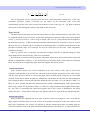
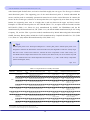
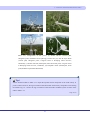
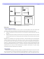
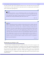
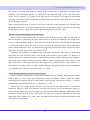
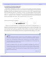
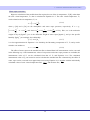
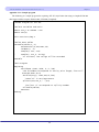
Observation of
Turbulence
Practical Handbook of Tower Flux Observation (Ver. 1.0)
Chapter 2
2.1 Ultrasonic anemometer thermometers (SATs)
When scalar fluxes are measured using the eddy covariance method, the fluctuating components of the
wind velocity need to be measured regardless of the type of scalar of interest. In the observation of the
fluxes across the interface between the Earth’s surface and the atmosphere, the vertical exchanges of
energy and scalar quantities are important. Therefore, flux observation requires measurements of the
fluctuating component of the vertical wind velocity (w [ms–1]), w' [ms–1]. In order to accurately estimate
the exchange of energy and scalar quantities by turbulence, the observation system needs to be capable of
measuring w' at a sampling rate of approximately 10 Hz or higher. The observation instrument also needs
to be able to make measurements without drifting on the time scale of at least several days and needs to be
durable enough to make field observations for a year to several years. Ultrasonic anemometer
thermometers (SATs hereafter) are currently the only sensors available that meet the above-mentioned
requirements.
Principle of measurement
The principle of measuring the wind velocity components and the sonic virtual temperature using a
SAT is explained below. A SAT measures the wind velocity and the speed of sound in the air, c, along the
straight line (path) between a pair of sensors (transducers) that face each other. The path length of a SAT
typically used in field observations (span length) is approximately 0.05 ~ 0.20 m. The pair of sensors are
internally equipped with transceivers made of acoustic elements. Acoustic signals are transmitted from one
transceiver to the other in both directions. From the time required for an acoustic signal to travel between
the transceivers in two directions, t1 [s], and t2 [s], the wind velocity component parallel to the path, vd
[ms–1] and the speed of sound, cs [ms–1] can be calculated from the following relationships. For the span
length of d [m], the travel times, t1 and t2 are expressed as
t1 =
d
d
, t2 =
cs + v d
cs − v d
(2.1-1a, 2.1-1b)
respectively. By subtracting the inverse of Equation 2.1-1b from that of Equation 2.1-1a, the following
relationship can be obtained to calculate vd:
vd =
d⎛1 1⎞
⎜ − ⎟
2 ⎜⎝ t1 t 2 ⎟⎠
(2.1-2)
By taking the sum of the inverse of Equation 2.1-1a and that of Equation 2.1-1b and using the
relationship between the speed of sound, cs, and the sonic virtual temperature, Tv [K]: cs = 403Tv , the
2
following equation can be obtained for calculating Tv:
28
2.1 Ultrasonic anemometer thermometers (SATs)
c2
1 ⎡ d ⎛ 1 1 ⎞⎤
Tv = s =
⎢ ⎜ + ⎟⎥
403 403 ⎣ 2 ⎜⎝ t1 t 2 ⎟⎠⎦
2
(2.1-3)
The air temperature can be calculated from the sonic virtual temperature measured by a SAT. The
calculation procedure requires corrections for the effects of the horizontal wind (cross-wind
contamination) and the water vapor content as described in a later section (pp. 38 ~ 39). Refer to Kaimal
and Gaynor (1991) and Hignett (1992) for the details of the corrections.
Types of SATs
The SATs that are generally used for field observations are three-dimensional SATs (3D-SATs). They
are equipped with three pairs of sensors, and the three orthogonal components of the wind velocity parallel
to the x, y, and z axes (or the u, v, and w axes) are output. (The z axis or w axis indicates the axis aligned in
the direction of gravity.)
Unlike one-dimensional SATs which measure the scalar flux in only the vertical
direction, the use of 3D-SATs allows calculations of momentum fluxes, coordinate transformations in the
post-data acquisition stage, and correction for the cross-wind effect on the sonic virtual temperature
acquired by the SATs.
There are various types of 3D-SATs. Commercially available 3D-SATs are durable enough for field
observations and are characterized by a fair level of reliability.
Specifications of well-trusted SATs that have often been deployed for observations both in Japan and
abroad are summarized in Table 2.1-1. The 3D-SATs that are frequently used in observations are classified
below according to the configuration of the frame that supports the sensors (probe).
Vertical path 3D-SATs
Some 3D-SATs measure the vertical component of the wind velocity with a pair of sensors that
constitute a path parallel to the vertical axis and measure the horizontal components of the wind velocity
with two pairs of sensors that lie in a horizontal plane. These 3D-SATs will be referred to as vertical path
3D-SATs in this section. When the paths are orthogonal to one another, the 3D-SATs are called orthogonal
type (orthogonal probe). Vertical path 3D-SATs include the TR-61A (Table 2.1-1), the TR-61C (Table 2.1-1,
Photo 2.1-1(a)), and the TR-90AH all manufactured by SONIC CORPORATION, Japan (former Kaijo
Sonic Corp.) and the "K" Style Probe (Table 2.1-1, Photo 2.1-1(b)) manufactured by Applied Technologies
Inc., US (ATI). (A measuring and control unit together with a TR-** probe is identified by the model
number DA-600.)
Of the probes listed above, the TR-61C and the "K" Style Probe are orthogonal probes.
Slanted path 3D-SAT
Some 3D-SATs are equipped with three pairs of sensors which are arranged in such a way that the
upper sensors of all three pairs are on the vertices of an equilateral triangle as are the lower sensors of all
three pairs. Furthermore, the sensors are attached so that the measurement paths are slanted from the
vertical axis and the center of the three measurement paths intersect. (See Photo 2.1-1.) These 3D-SATs are
29
Practical Handbook of Tower Flux Observation (Ver. 1.00)
Chapter 2
called slanted path 3D-SATs here, and can be classified roughly into two types. The first type is called an
omni-directional probe. The supporting post of the omni-directional probe is located underneath the
sensors, and the probe is rotationally symmetrical around an axis in the vertical direction. In contrast, the
sensors in the second type (referred to as boom probes here) are supported by arms from the top and the
bottom; the supporting arms meet at a height that is mid-way between the upper and lower sensors.
Examples of omni-directional probes are the TR-61B (Table 2.1-1; an option with the DA-600) and the
SAT-540/550 (Table 2.1-1, Photo 2.1-1(c)) manufactured by SONIC, the WindMaster and the R3
manufactured by Gill Instruments Ltd, UK. (Table 2.1-1), the Model 81000 manufactured by R. M. Young
Company, US, and the USA-1 (previous model) manufactured by Metek Meteorologische Messtechnik
GmbH, Germany. Boom probes include the CSAT3 manufactured by Campbell Scientific Inc, US. (Table
2.1-1, Photo 2.1-1(d)) and the HS manufactured by Gill (Table 2.1-1).
Tips!
Slanted path probes were developed subsequent to vertical path probes. Slanted path probes were
designed to minimize the disturbance of the horizontal wind, the magnitude of which is usually larger
than that of the vertical wind. However, because the three components of the wind velocity are
calculated from the outputs from all three sets of sensors, the failure of any one set of sensors may lead
to a loss of data for the sonic virtual temperature and all of the x-, y-, and z- wind velocity components
(Hirano and Saigusa, 2007).
Tips 2.1-1
Table 2.1-1 Specifications of widely-used SATs.
Manufacturer
Model/ probe
Path-length Configuration (angle between horizontal
plane and vertical-wind sensor path)
[m]★
Probe weight
[kg]
Output
Power
Flow distortion references
consumption
DA-600 (TR-61A)
0.2
Vertical path (90°; 120° between the
horizontal-wind sensor paths)
4.3
Digital / Analog
<30W
Kondo and Sato (1982), Hanafusa
et al . (1982), Wieser et al . (2001),
Ito et al . (2001)
DA-600 (TR-61B)
0.2
Slanted path, omni-directional probe (45°)
7.9
Digital / Analog
<30W
Wieser et al ., (2001)
DA-600 (TR-61C)
0.2
Vertical path, orthogonal probe (90°)
5
Digital / Analog
<30W
Wyngaard et al . (1985) ※1, ※2,
Shimizu et al . (1999) ※1, ※2,
Wieser et al . (2001)
SAT-540/550
0.1
Slanted path, omni-directional probe (45°)
2.7
Digital / Analog
4W
"K" Style Prob
0.15
Vertical path, orthogonal probe (90°)
<1.0
Digital
CSAT3
0.115
Slanted path, boom probe (60°)
1.7
Digital / Analog
WindMaster/
WindMaster pro
0.144
Slanted path, omni-directional probe (45°)
0.9 / 1.7(-pro)
Digital /
Analog (optional)
0.66W
van der Molen et al . (2004)※2,
Nakai et al . (2006)※2
R3(-50, 100)
0.144
Slanted path, omni-directional probe (45°)
0.9
Digital / Analog
3.6W
van der Molen et al . (2004)※2,
Nakai et al . (2006)※2
HS(-50, 100)
0.144
Slanted path, boom probe (48.75°)
2.5
Digital / Analog
3.6W
Cristen et al . (2001)
SONIC
ATI
Campbell
Gill
★ Even within the same model, the path length may differ by a few mm.
※1 Evaluation of transducer shadowing only,　※2 correction formula available
30
1.2W
None
Kaimal et al . (1990) (see also ATI
homepage)　※1, ※2
1.2 W (operating
Cristen et al . (2001)
at 20 Hz)
2.1 Ultrasonic anemometer thermometers (SATs)
(a)
(b)
(c)
(d)
Photo 2.1-1 Configuration of SAT probes: (a) SONIC TR-61C (vertical path,
orthogonal probe, Yamashiro forest hydrology research site), (b) ATI "K" Style Probe
(vertical path, orthogonal probe, evergreen forest in Kompong Thom Province,
Cambodia), (c) SONIC SAT-540 (slanted path, omni-directional probe, evergreen forest
in Kompong Thom Province, Cambodia), (d) Campbell CSAT3 (slanted path, boom
probe, Kahoku Experimental Watershed).
Tips!
All the 3D-SAT models in Table 2.1-1 output the upward vertical component of the wind velocity as
positive values. However, the sign convention of the horizontal wind velocity components varies among
the models. Fig. 2.1-1 shows the sign convention of the horizontal coordinate system of some of the
SATs in Table 2.1-1.
Tips 2.1-2
31
Practical Handbook of Tower Flux Observation (Ver. 1.00)
Chapter 2
y
x
ATI
"K" Style Probe
Campbell
CSAT3
SONIC
DA-600
x
y
x
Front side of the sensor
(For omni-directional probes,
side labeled with the letter “N”)
Gill
WindMaster
R3
HS
y
Back side of the sensor
Fig. 2.1-1 Sign conventions of widely-used SATs.
Deployment
Selection of deployment location
When a SAT probe is installed on a tower, in order to avoid the influence of the tower and the SAT
itself on the wind velocity measurements, the following precautions need to be taken into account:
1)
Deploy the SAT probe on the top of the tower or on a long boom to keep the SAT probe away from
the tower.
2)
Deploy the SAT probe pointing into the direction of the prevailing wind and the direction in which
the flow distortion by the tower and the probe itself is minimized. (Flow distortion will be discussed
on p. 37.)
Regarding 1), it is desirable to use a boom that is more than 1.5 times the width of the tower through which
wind passes (Hirano and Saigusa, 2007). When the use of such a boom is not feasible, deploy the SAT as
far as possible from the tower taking into account the tasks required for deployment and maintenance.
Caution 2) is especially important for the deployment of a SAT with a structure which disturbs the wind
flowing through the backside of the probe, e.g., the TR-61A and TR-61C manufactured by SONIC, the HS
manufactured by Gill, and the CSAT3 manufactured by Campbell. (The backside of a probe usually
corresponds to the side to which cables are connected.)
Probes and parts
In the process of deploying a SAT probe, fittings are required to attach the probe to the tower. In most
cases, the SAT probe (or the boom provided by the SAT manufacturer) is secured to a base by screws or
U-bolts. The base, in turn, is secured to the tower by half-clamps and/or U-bolts. The simplest base can be
32
2.1 Ultrasonic anemometer thermometers (SATs)
made by drilling holes in a flat plate. Because the size of the base and the positions of the holes depend on
the SAT and the tower specification, the investigator usually needs to build a base on his/her own. While
plywood is easy to fabricate, it can warp and deform. Thus, when the base is used for long-term
observation, metal such as stainless metal or aluminum is recommended for the base. Alternatively,
sufficiently dried solid timber can be used if appropriate corrosion protection is applied.
Some models of SATs come with signal converters that are separate from the probes. For these models,
additional installation space and fittings are required for the signal converters.
Tips!
The DA-600 (TR-61A, B, and C) manufactured by SONIC consists of a probe, a signal conversion box
(waterproofed), and an output unit (non-waterproofed). The CSAT3 manufactured by Campbell consists
of a probe and a signal conversion box (waterproofed). Waterproofed SAT components are usually
deployed outdoors while non-waterproofed SAT components are usually placed inside a sheltered space
such as a hut in which the components are protected from rainfall.
Tips 2.1-3
Cables
The signal cables of SATs are usually made of 5 to 20 cores, thus the weight of a signal cable can
become large depending on the length of the cable and the SAT model. (For example, the signal and power
cables of the DA-600 manufactured by SONIC weigh about 150 gm–1.)
It is desirable to determine the
appropriate cable length in advance so that it will not be heavier than necessary for hauling and handling.
Secure the bends in the cables to the tower with weather-resistant cable ties (e.g., Insulok,
HellermannTyton, UK) and vinyl tape while making sure that the bends in the cables do not get damaged
by vibrations caused by strong wind. Furthermore, secure the cables running along the tower at appropriate
intervals so that large tension loads are not placed on the cables themselves.
Leveling adjustment and tilt check
In principle, the SAT probe should be deployed in such a way that the z-axis component of the wind
velocity is parallel to the direction of gravity. (The x-y plane of the SAT probe is horizontal.) The time and
effort to adjust the leveling of the SAT can be reduced significantly if a simple level is added to the
above-mentioned base used for installing the SAT. (See above section on “Probes and parts”.) Nonetheless,
the horizontal deployment of a SAT may not be strictly feasible in some cases. When flux measurements
are made over sloped topography and the blow-up and blow-down angle of the wind velocity for the site is
known from preliminary measurements, the SAT may be tilted by that angle for deployment. In either case,
the tilt of the SAT should be measured with an inclinometer after the SAT has been stabilized; so that the
measured vales of the tilt can be used to correct the wind velocity and direction as necessary. Sometimes,
33
Practical Handbook of Tower Flux Observation (Ver. 1.00)
Chapter 2
the tower tilt or tower vibrations may be of concern because of the weight of workers on the tower or
strong wind, respectively. In this case, the use of a self-recording inclinometer is recommended to record
the tower tilt and/or vibrations.
Tips!
A bubble level is equipped on the probe of both the CSAT3 manufactured by Campbell and the DA600
(TR-61A) manufactured by SONIC. An inclinometer is built into the probes of the R3-100, R3A-100
and HS manufactured by Gill. (An inclinometer can be added as an option for the R3-100 or R3A-100.)
Tips 2.1-4
Data acquisition
The output values of a deployed SAT can be recorded by connecting its signal cable to a data logger
and setting the data logger appropriately. (For setting the data logger, refer to Section 2.6 “Data logger”.)
Depending on the model of the SAT, its output can be acquired either as an analog voltage signal or as
a digital signal. (Digital signal outputs can be acquired using the Campbell SDM port or the RS-232C port.
Many SAT models are able to output both analog and digital signals.)
An advantage of analog signals is
that they can be easily acquired and recorded by a large number of data loggers. On the other hand, an
advantage of digital signals is that the output values are subject to less noise than those acquired as analog
signals.
In Appendix 2.1-1, a sample program is given for acquiring digital data with a CR1000 from an ATI
"K" Style Probe. In this example, pin numbers 3 and 2 of the RS-232C connectors are connected directly to
the C1 and C2 ports of the CR1000, respectively. The sample program may serve as a useful reference for
recording digital data outputs from the SATs manufactured by SONIC or Gill. (However, there is no
guarantee that the program will work in all situations.)
When data from a CSAT3 are output digitally to a data logger such as a CR1000, an SDM cable can be
used for a simple and easy connection between the sensor and the data logger. The SDM connection
requires less electricity than other connections, and a sample program for the operation of the system is
available in the CSAT3 manual. Although the length of the SDM cable supplied by the manufacturer is
normally 7.62 m, the user may need to extend its length in some circumstances. In this case, the numerical
value in the parenthesis that follows the control command "SDMspeed" for Campbell data loggers needs to
be set to a larger value. (The numerical value used for SDMspeed is approximately 30 for an SDM cable
with a length of 7.62 m.)
34
2.1 Ultrasonic anemometer thermometers (SATs)
Tips!
SDM (Synchronous Devices for Measurement) is a protocol established by Campbell for improving
the communication control between a data logger and peripheral devices. Connection of a data
logger to peripheral devices via SDM enables synchronized data acquisition at a high speed.
Therefore, the use of SDM is suitable for measurements such as those for the eddy covariance
method in which multiple signals are acquired simultaneously at a high frequency and in which care
is necessary to correct for the mis-synchronization of the signals. The maximum communication
speed of SDM (SDM clock rate) changes according to the number of sensors that are connected, the
scan interval, and the cable length. Thus, according to the measurement system to be used, the SDM
clock rate needs to be set to an appropriate value in order to avoid communication errors.
Tips 2.1-5
Maintenance
Generally, a SAT requires very little maintenance after its deployment. Even when the coating material
on the SAT becomes discolored or peels off due to its deployment outdoors, the influence of these coating
modifications on the measurement result is extremely small if it exits at all. The data output can be
influenced by nearby lightning strikes or instantaneous power outages as well as rain drops within the
measurement paths or on the sensors. In these cases, the data output is characterized by abnormal values.
However, as long as no similar abnormality can be detected in the data from a few days without rain after
the occurrence of the abnormality, the SAT measurement can be continued without any adjustment. On the
other hand, if abnormal values occur intermittently and their cause is unknown, turn in the SAT to the
manufacturer for repair and replace it by a backup SAT immediately.
Unless data abnormalities such as those discussed above are observed, the following procedures are
sufficient for routine SAT maintenance:
・
If objects such as spider webs are in the SAT measurement paths, remove the objects.
・
If the surfaces of the sensors are extremely dirty, wipe them with a soft cloth wetted with alcohol or
distilled water.
In addition, in the case of a long-term SAT deployment, it is desirable to follow the procedures below
every few months to a year.
・
Check the wind velocity offset.
・
Correct the sonic virtual temperature by referring to the data collected by a thermo-hygrometer near
the SAT height.
・
Check if the tilt angle has changed from the time of deployment and adjust it if necessary.
Although it is recommended that the wind velocity offset be checked indoors, the offset can also be
checked on a SAT while it is still deployed. In this case, cover the SAT with a large plastic bag and check if
35
Practical Handbook of Tower Flux Observation (Ver. 1.00)
Chapter 2
the values of the three wind velocity components fluctuate near zero. If the offset values are large, the SAT
is likely defective; the data acquired after the offset check need to be examined quickly and carefully to
make a decision about repairing the SAT.
Tips!
The probe head of the TR-61 (A, B, C) manufactured by SONIC can be easily changed by the user.
When an abnormality arises on the TR-61, it can sometimes be resolved by replacing the probe head
which includes the sensors. Because a backup probe head is not as expensive as a SAT itself, it is
desirable to have a backup probe head ready when a TR-61 probe is used.
Tips 2.1-6
Tips!
Abnormal output data from SATs are frequently associated with the presence of raindrops. When the
probe of a slanted path SAT is deployed with its x-y plane perpendicular to gravity, the sensors are
tilted, and raindrops can slide off easily, which is considered an advantage of slanted path SATs.
Furthermore, as an option to guide raindrops away from the measurement paths, mesh fabric called
wicks can be placed on the sensors of the CSAT manufactured by Campbell. Due to their presence
around the sensors, wicks may become a source of additional disturbance for the wind in the vicinity
of the sensors. However, from the size of the wicks, it is speculated that their influence on the wind is
small. Although caution is necessary, wicks can be added and removed by the user. Therefore, it is
possible to use wicks only during the rainy season in which the influence of rainfall on the sensors is
expected to be large. In principle, the method of raindrop removal with wicks is also applicable to
SATs of any other manufacturers.
Tips 2.1-7
Measurement errors intrinsic to SATs
Errors associated with averaging over the measurement path
The wind velocity and signal speed (speed of sound) obtained by a SAT are those averaged over the
measurement path. Fine-scale fluctuations of a variable that occur at scales smaller than the path length are
averaged, i.e., path-length averaging effect or line-averaging effect. Fluctuations of a variable that occur at
finer scales than the path length are sometimes sought, for example, in the case of measurements
conducted near the ground surface. In such cases, a SAT which is equipped with short paths and a
non-orthogonal probe (i.e., a configuration in which multiple paths intersect at the same point in space)
should be utilized.
36
2.1 Ultrasonic anemometer thermometers (SATs)
The amount of missing high-frequency signals to be corrected due to path-length averaging varies
according to the atmospheric stability (e.g., Kristensen and Fitzjarrald, 1984). On the other hand, some
studies, such as Aubinet et al. (2000), report that sufficient corrections of the signals for path-length
averaging can be made with the comprehensive method proposed by Moore (1986) which does not depend
on the atmospheric stability.
When a slanted path 3D-SAT is used, the wind velocity and sonic virtual temperature are calculated from
the measurements made over the three paths of the SAT. For this reason, caution is necessary for correcting
missing high-frequency signals due to path-length averaging (Horst and Oncley, 2006).
Errors associated with SAT-induced flow distortion
When a SAT is used for observations, its probe is fixed in the wind velocity field. It is thus believed
that flow distortion is induced by the sensor and the frame of the SAT itself. Blockage of the wind by the
sensors is called “transducer shadow”. This effect becomes the main source of flow distortion when using
a vertical path probe in which two pairs of sensors are placed on a horizontal plane. On the other hand,
when a slanted path probe is used, it is likely that the supporting post and frame which support the sensors
induce flow distortion mostly in the vertical wind velocity.
Generally, flow distortion is evaluated using wind tunnel experiments. The results of wind tunnel
experiments for some of the SAT probes can be found in the references given in Table 2.1-1. However, it
remains controversial whether the results of wind tunnel experiments on flow distortion can be applied to
observational data collected in field experiments. While a number of applications of the results of wind
tunnel experiments to field observations have been reported (e.g., Kondo and Sato, 1982; Kaimal et al.,
1990; Nakai et al., 2006; Saitoh et al, 2007), studies opposing such applications have also been published
(e.g., Hanafusa et al., 1982; Ito et al, 2001; Ishida et al., 2004).
Model recommended for its small measurement errors
All the commonly used SATs have achieved an acceptable level of reliability. Particularly, the models
listed in Table 2.1-1 have earned good reputations in terms of reliability. Of these models, the CSAT3
manufactured by Campbell, due to its small intrinsic errors and high measurement accuracy, is currently
considered the most trusted SAT model (e.g., Mauder et al., 2007).
No formula is yet available for flow distortion correction for the CSAT3 that is based on a wind tunnel
experiment. Therefore, when flow distortion corrections are necessary for the measurements made by a
CSAT3, the investigator may need to conduct his or her own wind tunnel experiment. Furthermore, when
wind flows from the backside of the CSAT3 probe, the wind velocity field is disturbed by the boom that
supports the probe (Christen et al., 2001). Thus, the influence of the boom on CSAT3 measurements needs
to be taken into consideration.
37
Practical Handbook of Tower Flux Observation (Ver. 1.00)
Chapter 2
Correction of SAT-measured temperature
Correction of horizontal wind contamination
The variable cs in Equations 2.1-1 and 2.1-3 is strictly the speed of sound waves that are measured in
the path of a SAT. The actual distance traveled by the sound waves along the path becomes longer than the
path-length due to the wind component normal to the path (cross wind), vn [ms–1] (Kaimal and Finnigan,
1994). Accordingly, the values of cs in Equations 2.1-1 and 2.1-3 are smaller than the actual (true) speed of
sound, ct [ms–1]. The actual sonic virtual temperature, Tvt [K], is the temperature that is evaluated from the
value of ct. Therefore, in order to calculate Tvt, corrections are required for the cross-wind effect. The
following relationship holds between cs and ct with the presence of a cross wind, vn:
cs = c t2 − v n2
2
(2.1-4)
Therefore, the following can be obtained.
2
ct
1 ⎡d 2
⎢
Tvt =
=
403 403 ⎢ 4
⎣
⎛1 1
⎜⎜ +
⎝ t1 t 2
2
⎤
⎞
⎟⎟ + v n 2 ⎥
⎥⎦
⎠
(2.1-5)
When the sonic virtual temperature is evaluated from the vertical path of a vertical path 3D-SAT, vn is
equivalent to the horizontal wind velocity measured by the SAT. In this case, the cross-wind effect can be
corrected relatively easily. However, a somewhat complex method is necessary for the correction of the
cross-wind effect when slanted path 3D-SATs are used, particularly for the models in which the sonic
virtual temperature is evaluated from the measurements averaged over the three paths (Liu et al., 2001).
Tips!
Among the slanted path 3D-SATs in which the sonic virtual temperature is evaluated from the
measurements averaged over the three paths of an instrument, the CSAT3 manufactured by Campbell
outputs a sonic virtual temperature which has been corrected for the cross-wind effect. Furthermore,
concise procedures for correcting the cross-wind effect for the WindMaster, R3, and HS manufactured
by Gill can be found in their product manuals.
Attention: User Manual Issue 04 (April, 2009) for the WindMaster & WindMaster Pro states that the
virtual temperature output by the SAT has been corrected for the cross-wind effect. Whether the output
value of the virtual temperature has been corrected for the cross wind may depend on whether the data
are collected by an old or a new model. Thus, the investigator needs to inspect the manual for the
details on cross-wind correction.
Tips 2.1-8
38
2.1 Ultrasonic anemometer thermometers (SATs)
Water vapor correction
Rigorous calculation of the sensible heat flux requires the use of the air temperature, Ta [K], rather than
the sonic virtual temperature, Tvt, that is calculated in Equation 2.1-5. The sonic virtual temperature, Tvt,
can be related to the air temperature, Ta, as:
⎛
e⎞
Tvt = ⎜⎜1 + 0.32 ⎟⎟Ta
p⎠
⎝
(2.1-6)
where p [Pa] and e [Pa] are the atmospheric and water vapor pressures, respectively. If e << p ,
⎛
e⎞
⎜⎜1 + 0.32 ⎟⎟
p⎠
⎝
−1
≈1 − 0.32
m
e
e
e ; and also
0.32 ≈0.32
≈ 0.32q d ≈0.51q . Here, md is the molecular
mW
p
p−e
p
weight of dry air [kgmol–1], mW is the molecular weight of water vapor [kgmol–1], and q is the specific
humidity [kgkg–1]. Accordingly, the relationship
Ta = (1 − 0.51q )Tvt
(2.1-7)
is a close approximation for Equation 2.1-6. Similarly, the fluctuating components of Ta, Tvt, and q can be
related to one another as
Ta ' ≈ Tvt '−0.51Tvt q '
(2.1-8)
The effect of water vapor on the sensible heat flux evaluated from SAT measurements can be corrected
in the following way: if the instantaneous values of air pressure and water vapor pressure are available, the
instantaneous value of Ta can be calculated from that of Tvt and Equation 2.1-6. The calculated
instantaneous value of Ta can in turn be used to calculate the sensible heat flux. Alternatively, the effect of
water vapor can be corrected in an approximate sense using Equation 2.1-8 together with the individually
calculated values of sonic virtual temperature flux, w'Tvt ' , and moisture flux, w' q' .
39
Practical Handbook of Tower Flux Observation (Ver. 1.0)
Chapter 2
Appendix 2.1-1: Sample program
The following is a sample program for acquiring ATI "K" Style Probe data using a Campbell CR1000
data logger and the compact flash module, CFM100 (Campbell):
‘CR1000 Program for ATI SAT
'Declare Variables and Units
PUBLIC ATI_K as STRING * 100
PUBLIC SAT(4)
Units SAT=*ms-1/Deg C
'Define Data Tables
DataTable(Table1,1,-1)
DataInterval(0,100,mSec,10)
CardOut(1, -1)
Sample(4, SAT, FP2)
'
Sample(1, ATI_K, string)
'If activate, raw strings will be recorded
EndTable
'Main Program
BeginProg
SerialOpen (Com1, 9600, 0, 0, 500)
'The 3rd number corresponds to "Parity, Bits length, Flow ctrl"
Scan(100,mSec,10,0)
SerialIn(ATI_K, Com1,100,13,500)
'ASCII"13" is Carriage Return
SplitStr(SAT,ATI_K," ",4,0)
'The last “0” corresponds to split by number
CallTable(Table1)
NextScan
EndProg
40