Download Lean MAST - ThomasNet

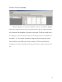
Lean MAST
User Manual
CMS Research, Inc.
1610 S. Main Street
Oshkosh, WI 54902
Tel: 920.235.3356
Fax: 920.235.3816
[email protected]
1
Table of Contents
Title
1.0 Modeling Factories
1.1 Add/Edit Factories
1.2 Create a Model
1.3 Open a Model
1.4 Import/Export Data
2.0 Model Building
2.1 Flow Route Data
2.2 Add Flow Centers/Stations
2.3 Part Details
2.4 Workcenter Details
2.5 Labor Team Availability
2.6 Batch
2.7 Station Reliability
2.8 Assembly
2.9 Disassembly
3.0 Capacity
4.0 Layout
4.1 Graphical Layout Definition
4.2 Visual Part Route
5.0 Simulation Analysis
5.1 Simulation
5.2 Graph Results
5.3 Gantt Charts
5.4 Animation
6.0 Cost Data
Page
3
4
5
6
7
8
9
10
11
13
15
16
17
19
20
21
23
24
26
27
28
29
30
31
32
2
1.0 Modeling Factories
Lean MAST provides an easy to use modeling tool to design and plan lean
manufacturing techniques through factory operations. Using the data collected from
process mapping, Lean MAST provides a “what if” configuration of Kanban sizes and
quantities, flexible labor teams, dedicated machines, and product flows. Lean MAST
provides the roadmap for the transformation from a work order based production system
to a production system that utilizes lean manufacturing techniques.
The benefits of Lean MAST are twofold. First, Lean MAST provides objective
analysis in finding the “best” solution for lean application. The “best” solution includes a
combination of machines, operators, inventory and processes that work with lean
manufacturing. Secondly, the use of Lean MAST leads to consensus. Having the
project team “on the same page” is essential for a successful transformation. Lean
MAST roadmap has resulted with many successful lean transformations.
This user manual is organized into six sections. There are model definitions,
model building, capacity planning, layouts, simulation analyses, and cost data. Each of
them is described in their own section.
3
1.1 Add/Edit Factories
Lean MAST provides a means to organizing models into separate factories. A
factory represents a group or set of models and has its own path name. All models in the
factory are stored in the corresponding directory and a factory must be defined before
any model can be saved or opened. To add a new factory, select Tools -> Edit
Factories
In the Manage Factories window, click the Add button to bring up the Specify a New
Factory window.
Create a name for the new factory and then click on the … button to specify the location
of the factory’s data. To edit a factory, highlight the name of the factory in the Manage
Factories window and click the Edit button. This will bring up the Specify a New
Factory window where the name and location of data can be changed.
4
1.2 Create a Model
Create a New Model
When Lean MAST starts a blank model appears. See Section 2.0 for model
building. When a second model is opened, then a second copy of MAST Lean-Sigma is
opened. Use the task bar to switch between models. The model name is printed at the
top of each window.
Copy a Model
Use File-> Copy model menu item. This opens a second MAST Lean-Sigma
session and then use File -> Save As to rename the copy with a different name. Use
factory selection to move models to other factory directories and backups.
Delete a Model
Use File -> Delete Model to remove a model from the factory directory.
5
1.3 Open a Model
To open an existing model, select File -> Open. This will launch the Open Model
window. Select the factory and highlight the model before clicking the Open button to
begin work in MAST Lean-Sigma
6
1.4 Import/Export Data
MAST Lean-Sigma provides an interface to comma delimited data. This format
has a fixed format where each column contains specific data. This format is used for
both export and import.
To prepare a template of the format for the comma delimited data is to use the
export of one of the sample models provided. This export file format can be opened in
Excel as a CSV file type. Model calculations can be done and saved in the CSV file type.
Then this file can be imported into a new model to bypass the need to enter flow route
data from the keyboard.
7
2.0 Model Building
The MAST Lean-Sigma model contains three types of data. These are flow route,
part details, and workcenter details. Each of these is described below.
8
2.1 Flow Route Data
Flow route data is added, edited, and deleted in the tab labeled Flow Route. Each
row in this table represents a product, component, or part. The user can choose the level
of detail for representation of products. It is recommended that initial studies begin with
”as high” a level of product definition as possible. The bill of material is collapsed to a
single level or only a few levels for major components and the flow routes represent the
total process time at these levels. Modeling strategies that use appropriate lending detail
are an important aspect that is part of the training course.
Each column on the table represents a flow center or place where a process
operation occurs.
9
2.2 Adding Flow Centers/Stations
Adding Flow Centers
Click the right button of the mouse to open an option window. This will provide
options to add, insert, or delete a column in the table. Once a column has been added,
then the name of the column will be the name of the flow center or station.
The data contained in the table is usually the total minutes of time required for the
product, component, or part represented in the row to complete the process identified in
the column. This time is a per piece time and Kanban sizes will automatically adjust for
total process time.
10
2.3 Part Details
The Part Details tab adds data to define each row in the flow route table. Each
product in the flow route has the production quantity defined. The top row of data boxes
define the planning period in terms of hours per day, number of days, and number of
shifts per day. The percent to simulate in the percentage of the planning period that the
simulation is to be run.
Kanban Definition
A Kanban is used to model a family for products/parts in the flow route. The
Kanban usually has a common flow or sequence of operations among its members.
Each Kanban is assigned a unique name, a size, and number of Kanbans. The
name is given to each flow that is to be modeled. [Hint: In the Flow Route text, each
column can be sorted by clicking on the operation name. This sort is maintained in the
part list in the product details tab. Kanbans can then be identified for groups of
products/parts that share the same operations.] The Kanban Size is the number of
products/parts that travel through the process as a single unit. This can be the batch size
and represents the number of individual parts that can be held in the Kanban container.
11
The number of Kanbans is the number of signal/containers that are allowed in the flow
loop. This generally is determined from the capacity tab results and is used in the
simulation. The inventory level is determined by multiplying the Kanban size by the
number of Kanbans.
Part Details
The part column contains term data. The quantity is the total number of pieces
required in production for the time horizon described above. Each part is then assigned
to a Kanban by selection from a deep-dorm box.
12
2.4 Workcenter Details
The Workcenter Detail tab is used to define labor teams, assign the teams to the
stations/flow centers, set the number of stations/machines in each flow center and set up
time and workcenter designation.
Labor Teams
Labor team is a group of operators who are assigned to a set of flow centers.
These operators can float to the stations as needed to perform flexible operations. Each
team is given a name and number of operators. The number of operators represents the
number of operators that are available each shift. The total number of operators is the
number of operations times the number of shifts.
Flow Centers
Stations/Flow Centers are defined with the number of stations, setup time,
assigned labor team, and work center designations. The number of stations is the
quantity of duplicate machines/work areas that are available to the parts. [Hint: Flow
modeling works best when stations that perform the processes are grouped into flow
centers. For example, five drills are best represented as one flow/center with five as the
13
number of stations. It is common to identify each drill as a single flow center but then
common product flows are not easily identified.]
Setup time is the one-time delay each time a new Kanban is delivered to the
station. This value is only used in simulation and does not influence capacity results.
A labor team is selected from the drop down box. Multiple options are available
to designate how the operations interact with the station. These designations are defined
in the Labor Time and Labor Type columns.
Labor Time and Labor Type
The Labor Type – Entire Operation designation is used when the operator is
required 100 percent of the time the station operates. This applies to fully manual
machines. The Labor Time field is not used.
The Labor Types – Start Only designation is used when the operator is needed to
load/unload a part, but the machine can operate on the part without the operator. The
Labor Time column designates the time the operator must be at the machine. The time in
the Flow Route Table designates the total cycle time for machine and external labor
times. A value for labor time less than one indicates a percent of the cycle time and a
value greater or equal to one designates the actual time.
The Labor Time – Maintenance designation is used when the operator is required at the
station only for setup and repair times. The Labor Time column is not used.
Workcenter
The Workcenter designation is used when two flow centers are routed as one or
the other or alternatives. Place a value of one in the column of the flow centers that can
be alternatives.
14
2.5 Labor Team Availability
Teams of operators (1 or more) are assigned to service a set of stations. Multiple
teams can overlap their service and serve the same stations. The list on the left indicates
each Team name and the number of operators on each team. The list on the right shows
the shift pattern, which describes the pattern of when the operator team is available and
unavailable. The Time column represents the length of time that an operator remains
either available or unavailable until the state is changed. The list also indicates the
accumulated time from the beginning of the pattern and the time range in hours for each
shift.
15
2.6 Batch
Each batch is described as a single screen and additional batches are described in
their respective screens. After the data is entered, the screen will refresh with the data for
the next batch. The batch data is terminated by entering a blank screen. To describe a
batch of parts, the Part ID entered must match that for a given part type. A list of part
IDs is shown in a vertical list to the left along with the production requirement for each.
If the ID does not patch, the response is ignored. A part type can be removed from a
batch by blanking out the Part response. When all parts have been removed from a batch,
the entire batch is deleted and the next one is brought in its place when window is closed.
The number of parts that are to be scheduled as part of this batch must be entered
in the Quantity column. If multiple parts are simultaneously loaded on a pallet, quantity
still reflects the number of individual parts.
16
2.7 Station Reliability
The Station Reliability tab allows the user to create and manage reliability
patterns. A Reliability Group is a user defined name for each reliability pattern. Each
station is assigned to a reliability group.
The list of feasible distributors is shown in the box on the left; when one is
selected, its name will be displayed along with the definition for its parameters. Each
distribution has from 1 to 4 parameters to describe its unique values for the specific
application. When the distribution has been identified, column headings will appear
indicating the specific parameters. These parameter values are time related, so they must
be expressed in the same units used in all previous time related data.
17
Efficiency and Repair Time
A simple solution to modeling random downtime cycles is to use the Uniform
distribution for both Failure and Repair. When the uniform distribution is selected for
both, the only two parameters that are needed are Efficiency Percent and Average Repair
Time. The Efficiency Percent is the percent of time when the status is to be available.
The Average Repair Time is the average time that the station is unavailable while being
serviced. The range for minimum and maximum parameters to the uniform distribution
equal to three times the average.
18
2.8 Assembly
This data describes the relationship between component parts that comprise
assembly parts. On the left side of the screen is a list of Assembly IDs. This is a list of
the part IDs described in the part description data. On the right is a column to enter the
Component ID. This response must be one of the part IDs described in the part
description. This response represents a component that is required to make an assembly.
Click on the Assembly ID that corresponds to the Component ID. Then enter the number
of the components that are required to make up an assembly in the Quantity column.
These screens repeat until a blank assembly ID is entered.
19
2.9 Disassembly
This data describes the relationship between component parts that comprise
disassembly parts. Each component must be described as a unique part type. The
components are not scheduled until the disassembly parts have been completed. On the
left is a list of Disassembly IDs. In the Part column, enter one of the part IDs described
in the part description. This response represents a component that is released from the
disassembly. Click on the corresponding Disassembly ID. In the Quantity column, enter
the number of components that are released from the disassembly.
20
3.0 Capacity
The capacity analyses in Lean MAST contain four components: The Production
Capacity is a list of Kanbans and the details of the parts arranged to each Kanban. The
blank line contains all parts not assigned to a Kanban. The Total Hours column is useful
to compare volume of flow for each Kanban.
The Inventory shows for each Kanban the quantity defined, the average required,
and estimated flow cycle time.
The average and flow time are determined by approximation to a solution of
Little’s Law (P=I/F). These average and flow times are estimates useful in sizing staging
areas and inventory levels.
The Labor Team and Station Loading is a list of labor teams showing target use.
The detail for each labor team shows the list of stations and its loading level. Any word
21
level over 100% is not feasible to achieve. The highest level represents the bottleneck of
the process.
The Production Rate-Inventory graph shows solutions to Little’s Law (P=I/F) for
all inventory levels. The point on the graph shows the current results and changing the
planning Luzon can change the focus along the curve.
22
4.0 Layout
The layout adds the specific orientation of the station and distances to the process
data. The comprehension of layout data and process data are required for simulation.
The Layout button opens the layout definition window. The flow route diagram
opens the layout window and allows the visual view of part flow through the graphical
layout.
23
4.1 Graphical Layout Definition
The definition of a graphical layout is done with a three step process.
Step 1 (Optional): Import CAD drawing.
a. Click Editing MAST Objects button to switch to Editing Other Objects
mode.
b. Use file menu – load drawing menu items.
c. Select file name that contains CAD image.
[Note: Only AutoCAD version 12 DXF format file works best.
Use CAD software to store drawing in this format before importing
to MAST Lean-Sigma.]
Step 2: Add Track Section
a. Click to Editing MAST Objects mode. (Button in Right hand side must
24
be enabled).
b. Click on Add Trk. Sec. button.
c. Select Flow and click OK.
d. Enter total distance, click OK.
e. Click on screen for left point or beginning of track section (aside).
f. Click on screen for right point or end of track section (aside)
Step 3: Add Stations
a. Click on Add Station button.
b. Select station from list, click OK.
c. Select location above/below, left/right of track, click OK.
d. Click location of delivery point for the station. This point must be
located on a track section.
e. Select a symbol for the footprint of the station. (This can be cancelled
if a CAD drawing was imported.)
f. Click the location of the work tables for the station. The point is used
for animation when a part has an operation performed at the
station. This point can be located anywhere on the screen.
g. Click the location where the operator stands when working at the
station.
Use File menu – Save to save the drawing. CAD and edit features are available.
25
4.2 Visual Part Route
Select a part or list of parts in the right corner list. A line flow of the operation
sequence is drawn in the layout. The thickness of the lines indicates the volume of flow.
26
5.0 Simulation Analysis
Simulation analysis is contained in the flow tabs: Simulation, Graph Results,
Gantt Charts, and Animation. The Simulation requires the process data and layout. The
layout must contain at least one track section and all stations must be located on a track
section. Track sections must be intersected so any part sequence of operation have a
defined traffic flow.
Simulation results only appear when a layout has defined flow through all
operations.
27
5.1 Simulation
The simulation is run as needed when the tab is opened. The simulation results
are shown in four sets of data.
Production Summary shows the list of parts and completed production. Each day
shift has its own set of data and this is selected from the left hand column.
Inventory Summary shows the average use and cycle time for each Kanban.
These will not exceed quantity available set in the Product Details Tab. Labor and
Station Use Summary compare the target load to actual use levels.
Cart Summary shows the average time each cart spends moving, waiting, and
unavailable during the simulation. The total number of assignments each cart completes
also appears along with the average time each assignment took. An assignment is
defined as a request to pick up and drop off a pallet.
28
5.2 Graph Results
Each item can be graphed to show the percent of time the item was busy or
occupied during the simulation. A graph can also be constructed for each task to show
the percent of tasks completed at any point in time during the simulation. To view a
specific graph, click on the item in the window directly to the right of the chart.
29
5.3 Gantt Charts
A Gantt chart is a visual schedule of productivity. Each line represents a different
machine. The width of each block represents the time each part spends on that machine
and the color and hash code of each block represents a different part. Using the color and
hash code, a part can be tracked to show how much time it spends at each machine.
30
5.4 Animation
The Animation tab shows the movement of parts, Kanbans, and operators through
the layout. This is a play back of the simulated operation that produced the performance
statements. Select a part from the list and click the Run Animation button to view an
animation for a specific part.
31
6.0 Cost Data
Cost Data tab is used to calculate actual best absorption of each part. Annual
Station Costs are entered to represent the operating cost and depreciation. Labor is
defined as an hourly cost. Operating costs are listed with annual cost. Then costs are
totaled and the actual production rates and mix are used to calculate 100% absorption of
this cost. Less than 100% absorption of cost can be set by using manual efficiency
percent overrides.
32
Educating and Integrating Lean Project Members
1610 S. Main Street
Oshkosh, WI 54902
Tel: 920.235.3356
Fax: 920.235.3816
[email protected]
33