1
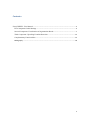
FuzzyUPWELL System v2.2 Computacional system for the automatic detection of upwelling from sea surface temperature (SST) images via Fuzzy Clustering User Manual Yashu Chamber1, Susana Nascimento1,2 1 Centre of Artificial Intelligence, Universidade Nova de Lisboa 2 Departamento de Informática, Faculdade de Ciências e Tecnologia, Universidade Nova de Lisboa 2011 Contents FuzzyUPWELL User Manual ....................................................................................................... 3 First Component: Initial Settings .............................................................................................. 4 Second Component: Visualization of Segmentation Result...................................................... 7 Third Component: Upwelling Frontline Detection ................................................................. 12 Complementary Functionalities .............................................................................................. 15 Bibliography ............................................................................................................................ 18 2 FuzzyUPWELL User Manual The FuzzyUPWELL tool has three main components: 1) The first component corresponds to dataset loading, clustering algorithm selection, parameter setting, and algorithm execution. 2) The second component provides functionalities on visualization of clustering results. 3) The third component corresponds to the upwelling frontlines detection, their visualization, and analysis. Figure 1. A screenshot of FuzzyUPWELL tool 3 First Component: Initial Settings Figure 2. Setting the initial parameters for a loaded image, and applying a clustering algorithm 1) The dataset can be loaded using the push button ‘Load New SST Map’. The loaded image is displayed in the left hand axis. A color bar corresponding to the loaded SST image is displayed on its right. The color bar temperature range is set to default (12ºC to 24ºC). By pressing the ‘Specific colorbar scale’ button the color bar temperature range will be set according to the maximum and minimum temperature values of the loaded dataset. A slider below this axis changes the color palette of the loaded image. 2) Once the SST dataset is loaded, the user is either required to select a clustering algorithm and set the associated parameters using Option 1 panel, or, to load a result file (if available) using ‘Load Result File’ push button. This file contains the fuzzy segmentation of the clustering algorithm applied to the loaded SST image, which was saved for this dataset during a previous run. This functionality is useful since loading the result file is much faster than applying the clustering algorithm to the SST image. 4 3) The clustering algorithms currently present in the FuzzyUPWELL tool are: (i) Anomalous Pattern Fuzzy Clustering (AP-FCM), (ii) Fuzzy C-means (FCM), and (iii) Histogram Thresholding. (i) The Anomalous Patter Fuzzy c-Means (AP-FCM) is the novel fuzzy clustering algorithm described in the paper (Nascimento and Franco,2009b). The user has to select a termination criteria for this algorithm. The available options are: (1) APC1 which ensures that the clustering terminates only when all data points have been clustered; (2) AP-C2 which terminates the clustering when the contribution to the data scatter of the last cluster obtained becomes smaller than a pre-defined threshold. An empirically tested threshold value is already set, however the user has the option to change to a different value; (3) AP-C3 which halts clustering when number of clusters has reached a pre-defined maximum value. (ii) The Fuzzy c-Means (FCM) is the second clustering algorithm (Dunn, 1973), (Bezdek, 1981). For this algorithm, the user has to pre-specify the number of clusters to be found. (iii) The Histogram Thresholding (Tobias and Seara, 2002) is the third clustering algorithm. On choosing this algorithm the user also has to pre-specify the number of clusters to be found. 4) After an algorithm is selected, the clustering of loaded SST image can be started using the following push buttons: a. ’Apply’ button (recommended), which starts by searching for a possible existing clustering result on the default directory according to the algorithm selected, if present in the default directory it will load the result which is useful since it is faster than applying the algorithm. If not, the tool will execute the chosen clustering algorithm, saving the clustering result in the default directory. 5 b. ‘Apply Algorithm’ button applies the chosen algorithm to the SST dataset, independently of whether the clustering result is present or not in the default directory.. Alternatively, if there is a large number of SST images in the same directory and the user wishes to apply a specific clustering algorithm to all at once and interruptedly, the user can choose the ‘Apply for all Images’ button. In this case, the user selects a clustering algorithm, a directory where the datasets are stored (using the ‘Load Folder’ button in the top left corner), and a directory where the clustering results are to be saved. The default directory is recommended to gain full advantage of the Apply button. Figure 3. How to apply a specific clustering algorithm to a set of SST images. 6 Second Component: Visualization of Segmentation Result Once the SST image is segmented and the result is available, it can be visualized and analyzed in following ways: 1) Fuzzy Membership Map: This option displays the fuzzy membership map assigned to a clustering segmentation. These degrees of memberships are visualized by assigning a color value to the data pixels based on their maximum membership value (Nascimento and Franco, 2009a). Figure 4. Visualizing a fuzzy membership map after applying a fuzzy clustering algorithm to an SST image. 7 2. Cluster Borders: The cluster borders can be visualized using different criteria: 2.1 Crisp criteria displays the original SST image with cluster borders marked on it. Figure 5. Visualizing Crisp cluster frontlines 2.2. The other criteria are the uncertainty measures which enable to visualize the classification uncertainty with which pixels are assigned to clusters after defuzzification, these are: (i) Fuzzy-Ignorance Uncertainty (ii) Fuzzy-Exaggeration Uncertainty (iii) Fuzzy-Confusion Ratio (iv) Fuzzy-Confusion Difference. 8 Figure 6. Visualizing the fuzzy frontlines using the ‘ignorance uncertainty’ measure (ii) Fuzzy-Ignorance Uncertainty is an entropy measure which is used to measure ignorance uncertainty associated with the defuzzification process assigned to each pixel of an image. This measure will be higher for values where the memberships are highly dispersed for all clusters, such as membership values of [0.3; 0.37; 0.33], and lower for memberships where the entity is highly associated with a single cluster, such as [0.1;0.84;0.06]. (iii) Fuzzy-Exaggeration Uncertainty is a measure associated with the hardening of a classification. It means that this is the uncertainty associated with the maximum membership of each entity. This way, the measure will be higher for entities with lower maximum membership values, exaggerating the fuzziness of segmentation. Both of the above measures lie between 0 and 1. The 0 value means that each entity has full membership to the cluster it is assigned to, i.e. zero uncertainty; The 1 value means that each entity has an equal degree of membership to all K clusters, i.e. complete uncertainty. 9 (iv) Fuzzy-Confusion Ratio is the ratio between the second highest membership and the highest membership for each pixel. For example, if the highest membership of a pixel is to cluster 1 with value 0.823 and the second highest membership of the same pixel is to cluster 2 with value 0.156, then the Fuzzy-Confusion Ratio for that pixel would be 0.1560/0.823 = 0.1896. The lower this value for a pixel, the lower it’s fuzzy nature. (v) Fuzzy-Confusion Difference is equivalent to 1 - (Difference between the highest membership and the second highest membership). The lower this value, the lower the fuzziness of data entity. The fuzzy boundaries obtained by the uncertainty measures described above can be visualized by distinct levels of opaqueness on the segmented SST image by using different parameters. The ‘Alpha-value’ slider enables to change the lower threshold for identifying the frontline pixels; the ‘Opaqueness’ slider enables to set the degree of opaqueness of the fuzzy frontline pixels. Separate frontlines can be viewed using the options: 1) View All frontlines, 2) View First 3 frontlines, 3) View a specific frontline, 4) View Upwelling frontlines, or 5) View Upwelling Front. The last two options (4 & 5) become available only after the upwelling front detection routine is run (as described in the next component). 10 Figure 7. Visualizing the first 3 fuzzy borders along with crisp boundaries. The range of mean temperatures of the fuzzy borders is displayed on the right hand side in ‘Frontline Temperature’ panel 11 Third Component: Upwelling Frontline Detection The ‘Upwelling Frontline Detection’ panel is used to set parameters for identifying the upwelling frontlines. A default parameter setting is available, which has been tested for the years on 1998 and 1999. This current parameter value computes the upwelling front with high accuracy for SST images of these two years. Naturally, the user has the option to change these default values. Figure 8. Upwelling front is detected using the Information Gain algorithm. The Upwelling front minimum and maximum temperatures and mean cluster’s temperatures are also shown. 12 There are 3 modes for detecting the upwelling front: 1) In Experimental mode, the parameter values have been manually fixed such that the results were best matched with the analysis of the oceanographers. These fixed parameter values works correctly in almost all images. 2) In Information Gain mode, the threshold value of each feature, TDiff and Cluster Extension, has been established using an entropy-based attribute discretization procedure (Nascimento and Franco, 2009b) 3) In Custom mode, the user sets the parameter values. The Parameters are TDiff South, TDiff North, Cluster Extension and Cloud Noise. (i) TDiff South denotes the threshold value of relative temperature difference between consecutive cluster prototypes in the southern region (below Cabo Espichel or 38.42 N latitude). This threshold is used to compute the transition cluster of the upwelling region in the south. This parameter setting is specifically for detecting upwelling in Coastal Portugal. For other regions, these parameters could be manually set by the user using the Custom mode. (ii) TDiff North denotes the threshold value of relative temperature difference between consecutive cluster prototypes in the northern region (above Cabo Espichel or 38.42 N latitude). This threshold is used to compute the transition cluster of the upwelling region in the north. This parameter setting is specifically for detecting upwelling in Coastal Portugal. For other images, these parameters could be manually set by the user. (iii) Cluster Extension denotes the cardinality of the pixels belonging to the upwelling region. This parameter is used to set the upper limit on the percentage of the area that can be covered by upwelling. (iv) Cloud Noise denotes the number of pixels in the upwelling region neighboring the clouds. This parameter sets the upper limit of the number of pixels in the upwelling region that can border the clouds. If the number of pixels 13 surrounding clouds is greater than ‘Cloud Noise’, the upwelling transition cluster number is decreased by one. After delineating the upwelling total area, it can be visualized and analyzed using either ‘Feature Panel’ push buttons, or using ‘View Upwelling Borders’ and ‘View Upwelling Front’ options under Fuzzy-Ignorance Uncertainty / Fuzzy-Exaggeration Uncertainty / FuzzyConfusion Ratio / Fuzzy-Confusion Diff> Border Type. 14 Complementary Functionalities The tool provides a set of additional functionalities, which are: Figure 9. Visualizing fuzzy upwelling front boundary. Upwelling front minimum and maximum temperatures and mean cluster temperatures are also shown. Useful options for manipulating the image is also highlighted in Feature Panel 1) The Mean Temperature panel which displays the mean temperature of each cluster. The colors in front of the clusters’ numbers identify the mean temperature of the corresponding cluster and correspond to the color bar in the Result Axis. 2) The Frontline Temperature panel displays the minimum and maximum temperatures of the fuzzy frontlines between neighboring clusters. Once again, the color assigned to the temperature values correspond to the color by which the borders are visualized on the Result Axis. 15 3) The Feature Panel consists on several options to visualize the clustering results and extract useful information. Specifically: (i) ‘Save Results’ button which saves the segmentation result of a clustering algorithm to a file; (ii) ‘Extract Image’ button, which provides a screenshot of the image, such that it can be analyzed separately; (iii) ‘Upwelling Area’ button, which shows the upwelling structure retrieved from the segmented image (and after the Front detection (iv) ‘Upwelling Front’ button, which allows to visualize the upwelling front in the right axis individually; (v) ‘Save Info Upwelling Front’ button, which saves into a file the spacial and geographical coordinates of the pixels in the upwelling front, as well as their distance to the coast line Figure 10. After pressing the Upwelling Area button the user visualizes the upwelling area. The Restore STT Image allows the user to view to the previous image 16 Figure 11. After pressing the Upwelling Front button the user visualizes the upwelling front boundary apart from the remaining cluster frontlines. The Restore button allows the user to view the previous image 17 Bibliography Susana Nascimento, Pedro Franco, Fátima Sousa, Joaquim Dias, Filipe Neves (2012). “Automated computational delimitation of SST upwelling areas using fuzzy clustering”, Computers & Geosciences, Volume 43, pp. 207–216, Elsevier, June 2012, (http://dx.doi.org/10.1016/j.cageo.2011.10.025) S. Nascimento, P. Franco (2009b), “Unsupervised Fuzzy Clustering for the Segmentation and Annotation of Upwelling Regions in Sea Surface Temperature Images”, in: J. Gama (eds), Discovery Science, LNCS 5808, Springer-Verlag, Vol. 5808/2009, Pag. 212-226, Porto, Portugal, October 2009. S. Nascimento, P. Franco (2009a), “Segmentation of Upwelling Regions in Sea Surface Temperature Images via Unsupervised Fuzzy Clustering”, in H. Yin and E. Corchado (Eds.), Proc. of the Intelligent Data Engineering and Automated Learning- IDEAL 2009, LNCS 5788, Springer-Verlag, pp. 543–553, Burgos, Spain. P. Franco, (2009). MSc Thesis. Fuzzy clustering não supervisionado na detecção automática de regiões de upwelling a partir de mapas de temperatura da superfície oceânica. Faculdade de Ciências e Tecnologia‐ Universidade Nova de Lisboa (in Portuguese). 18