1
Verification Condition Splitting
K. Rustan M. Leino 0 , Michał Moskal 1 , and Wolfram Schulte 0
0
Microsoft Research, Redmond, WA, USA
{leino,schulte}@microsoft.com
1
University of Wrocław, Poland
and European Microsoft Innovation Center, Aachen, Germany
[email protected]
Manuscript KRML 192, 10 October 2008.
Abstract. In a traditional approach to program verification, the correctness of
each procedure of a given program is encoded as a logical formula called the
verification condition. It is then up to a theorem prover, like an automatic SMT
solver, to analyze the verification condition in the attempt to either establish the
validity of the formula (thus proving the correct correct) or find counterexamples
(thus revealing errors in the program). This paper presents a technique that, via
program-structure-aware transformations that split one verification condition up
into several, lead to better overall performance of the SMT solver, sometimes
making it up to several orders of magnitude faster. The technique also lends itself
to improved error messages in case of verification failure due to time-outs.
0
Introduction
Verification-condition generation offers a straightforward way to harness the power of
a theorem prover in program verification: first, encode the program’s correctness conditions as a logical formula, called the verification condition (VC), and then, use the
theorem prover to analyze this formula. If the theorem prover can establish the validity
of the formula, then it has proven the program correct; if it finds a counterexample to the
given formula, then it has discovered an error in the program; if the theorem prover runs
out of steam, for example by exhausting its search strategies or reaching some resource
limit, then the program verifier reports an inconclusive result, possibly in the form of a
spurious error message. This general architecture has been the basis for many program
verifiers, for example the Stanford Pascal Verifier [12] and the Extended Static Checker
for Modula-3 [7] and Java [9].
To support modular verification, the process of VC generation is applied separately
to each part of the program, traditionally at the level of each procedure (cf. [14]). A welcome consequence thereof is that it makes program verification linear (in terms of time
and other resources consumed) in the number of procedures in the program. Unfortunately, each procedure can take a long time to verify. During our work with verifying
Spec# [3, 5] and C [1] code, we have found numerous methods where the current stateof-the-art SMT solver [6] took very long (i.e., hours up to what would have been days)
to come back with an answer. The usual cycle of developing verified code involves iterative calls to the program verifier, intermixed with slight changes in specifications or
code. For this cycle to be effective, we need verification times measured in minutes or
preferably milliseconds, not days. In this paper, we explore a way to reduce the time
taken to verify each procedure.
Our general idea is to split the verification condition of a procedure into several
verification conditions, whose conjunction is equivalent to the original one. Ideally, a
theorem prover would be able to prove a formula φ ∧ ψ in the same time that it takes
it to prove φ and ψ separately. In fact, it is not outrageous to think the prover could
prove φ ∧ ψ faster than φ and ψ separately, because proving one conjunct may lead
to the discovery of lemmas that are useful in the proof of the other. However, we have
observed that while in most cases proving φ ∧ ψ together takes less time then proving
them separately, it is sometimes the case that the SMT solver can prove each of φ and ψ
in a very short time, but proving φ ∧ ψ can be orders of magnitude slower. Our observed
phenomenon is particularly pronounced for larger VCs. It is hard to pinpoint the exact
cause for such crosstalk (even with the help of the authors of the SMT solver), but
one can speculate that, for example, the conjunction gives rise to unfruitful quantifier
instantiations that in turn lead to a plethora of new case splits.
More specifically, our idea is to split VCs using control-flow information. This may
be a win over more arbitrary formula splitting if, for example, the lemmas discovered
during the proof of one proof obligation turn out to be useful also for other proof obligations in the same branch of the program. Because we want to use control-flow information, we perform the splitting already at the level of the intermediate representation of
the program, before the logical formula has been generated and passed to the theorem
prover. The correctness of our technique, which we establish in Section 2, hinges on the
fact that the union of the execution traces of the split procedure equals the execution
traces of the original procedure.
We have implemented our technique in the Boogie verification system [3], which is
used as the underlying proof engine for several program verifiers, including the Spec#
verifier and verifiers for C (Havoc [0] and VCC [1]). Our technique improves performance, in some cases up to several orders of magnitude (see Section 4). Furthermore,
our technique allows us to output improved error messages in case of verification failure
due to time-outs.
The contributions of this paper are thus
– a formalization of the VC split concept along with soundness and completeness
proof (Sect. 2)
– heuristical methods that specify how to choose a split and when to split (Sect. 3)
– a detailed performance evaluation of VC splitting (Sect. 4)
1
Definitions
We assume the existence of a theory used to interpret verification conditions. The language T of the theory is assumed to be closed under boolean connectives with the
usual interpretations. The meta-variables ψ and φ refer to formulas of the theory (i.e.,
ψ, φ ∈ T ), the notion M φ means the formula φ is true in model M .
The procedure is presented as control flow graph (CFG), which is a quadruple G =
(V , E , e, L), where V is finite set of vertices, E ⊆ V × V is the set of edges, e ∈ V
2
is the entry point and L : V → L is the labelling function. The set of labels is defined
as:
L ::= assume φ | assert φ
+
We use the notion n0 → n1 for (n0 , n1 ) ∈ E . Let · → · be the smallest transitive relation
E
E
∗
+
E
E
containing · → · and · → · smallest reflexive relation containing · → ·. Let R(E , n) be
E
∗
the set of nodes reachable from n , i.e. n 0 ∈ R(E , n) iff n → n 0 . We put the following
E
requirements on CFGs:
+
– acyclicity, i.e. there does not exist n ∈ V such that n → n
E
– all vertices should be reachable from entry, i.e., V = R(E , e) (it follows that there
are no edges ending in e )
The set of all CFGs is denoted G . For a given G ∈ G , where G = (V , E , e, L), we
define:
φ
when L(n) = assume φ
condG (n) =
true
otherwise
(
true
when n = e
preG (n)
= W 0 (pre (n 0 ) ∧ condG (n 0 ))
otherwise
G
n →n
E
preG (n) ∧ ¬φ when L(n) = assert φ
wrongG (n) =
otherwise
W false
wrong(G) = n∈V wrongG (n)
We say the program represented by a CFG G goes wrong, iff there exists a model M ,
such that M wrong(G). We imagine that M represents an execution trace, preG (·)
is the condition that execution trace has to fulfil at the entry of the node and wrongG (·)
is the condition saying that the assertion fails in given execution trace. The execution
trace also includes the path that lead to a failed assertion. This intuition is captured by
the following lemmas. Let:
_
ˆ G (n) =
pre
condG (n0 ) ∧ . . . ∧ condG (nk −1 )
e=n0 →n1 →...→nk =n
E
E
E
ˆ G (n).
Lemma 1. For every n ∈ V , such that n 6= e , M preG (n) iff M pre
Proof. By induction on the length of the longest path from e to n .
t
u
Lemma 2. For every n ∈ V , M wrongG (n) iff there exists a path e = n0 →
E
n1 → . . . → nk = n such that L(n) = assert φ and M condG (n0 ) ∧ . . . ∧
E
E
condG (nk −1 ) ∧ ¬φ.
For a graph G that goes wrong, the path and model from Lemma 2 are called the
offending path and the offending model.
A correct split of of a CFG G into CFGs G0 and G1 is one where M wrong(G)
iff (M wrong(G0 ) ∨ M wrong(G1 )).
3
2
A Split
Let L S be the labelling function, where the asserts are only checked in S , i.e.:
assume true when L(n) = assert φ and n ∈
/S
L S (n) =
L(n)
otherwise
Lemma 3. Let G = (V , E , e, L) and G 0 = (V 0 , E 0 , e, L S ), where V 0 ⊆ V and
E 0 ⊆ E (G 0 is subgraph of G ). Any offending path and model in G 0 will also offend
G.
Proof. Any path in G 0 also exists in G . Moreover for every n ∈ V 0 we have condG (n) =
condG 0 (n). For the last node n on the offending path, we have L S (n) = assert φ
and thus also L(n) = assert φ.
t
u
We restrict ourselves to CFGs where each node has at most two exits. Any CFG
G can be transformed into such, while preserving wrong(G), by adding additional
two-exit nodes labeled with assume true .
A horizontal split of a CFG G = (V , E , e, L) is created by choosing a node n
with two exits n0 and n1 (i.e., n0 6= n1 , n → n0 and n → n0 ) and creating two CFGs,
E
E
G0 and G1 , such that:
V0 = R(E \ {(n, n1 )}, e))
G0 = (V0 , E ∩ V0 × V0 , e, L)
V1 = R(E \ {(n, n0 )}, e)
G1 = (V1 , E ∩ V1 × V1 , e, L R(E ,n1 ) )
That is, for G0 we remove n → n1 and every nodes that become unreachable and for
E
G1 we remove n → n1 and every nodes that become unreachable, as well as all assert
E
nodes “above” n . We show an example of a horizontal split of the CFG in Fig. 0.
Theorem 1. Horizontal split of G into G0 and G1 is correct.
Proof. If G goes wrong, then consider its offending path and model. (0) If the path
contains edge (n, n1 ) then it does not contain (n, n0 ) (the graph is acyclic), so the
path is also present in G1 . The last node on the path is reachable from n1 , thus the
assert is still present in L R(E ,n1 ) . Therefore the same path and model will offend G1 .
(1) Otherwise, as the edge (n, n1 ) is not used, the path is present in G0 . The final assert
is untouched (we do not cut the labelling function for G0 ) and thus the path and model
will offend G0 .
Conversely, both G0 and G1 are subgraphs of G in the sense of Lemma 3.
t
u
For a set S ⊂ V , the vertical split of CFG G = (V , E , e, L) is:
G0 = (V , E , e, L S )
G1 = (V , E , e, L V \S )
Theorem 2. Vertical split of G into G0 and G1 is correct.
Proof. If the offending path of G ends in S then it will offend G0 , otherwise it will
offend G1 . Conversely, again both G0 and G1 are subgraphs of G .
4
uint find_zero(uint m)
requires(exists(uint k;
ensures(f(result) == 0)
{
for (uint i = 0; i < m;
invariant(forall(uint
{
if (f(i) == 0) return
}
assert(false);
}
assume 𝜓
k < m; f(k) == 0))
i++)
j; j < i; f(j) != 0))
i;
∃ 0 ≤ 𝑘 < 𝑚. 𝑓 𝑘 = 0
∃ 0 ≤ 𝑘 < 𝑚. 𝑓 𝑘 = 0
∃ 0 ≤ 𝑘 < 𝑚. 𝑓 𝑘 = 0
𝑖0 = 0
𝑖0 = 0
𝑖0 = 0
∀ 0 ≤ 𝑗 < 𝑖0 . 𝑓 𝑗 ≠ 0
∀ 0 ≤ 𝑗 < 𝑖0 . 𝑓 𝑗 ≠ 0
𝑡𝑟𝑢𝑒
∃ 0 ≤ 𝑗 < 𝑖1 . 𝑓 𝑗 ≠ 0
∃ 0 ≤ 𝑗 < 𝑖1 . 𝑓 𝑗 ≠ 0
∃ 0 ≤ 𝑗 < 𝑖1 . 𝑓 𝑗 ≠ 0
𝑖1 < 𝑚
¬(𝑖1 < 𝑚)
assert 𝜓
Legend
¬(𝑖1 < 𝑚)
𝑖1 < 𝑚
𝑓 𝑖1 = 0
¬(𝑓 𝑖1 = 0)
𝑟𝑒𝑠𝑢𝑙𝑡 = 𝑖1
𝑖2 = 𝑖1 + 1
𝑓𝑎𝑙𝑠𝑒
𝑓 𝑖1 = 0
¬(𝑓 𝑖1 = 0)
𝑟𝑒𝑠𝑢𝑙𝑡 = 𝑖1
𝑖2 = 𝑖1 + 1
∀ 0 ≤ 𝑗 < 𝑖2 . 𝑓 𝑗 ≠ 0
𝑓 𝑟𝑒𝑠𝑢𝑙𝑡 = 0
𝑓𝑎𝑙𝑠𝑒
∀ 0 ≤ 𝑗 < 𝑖2 . 𝑓 𝑗 ≠ 0
𝑓 𝑟𝑒𝑠𝑢𝑙𝑡 = 0
𝑓 𝑟𝑒𝑠𝑢𝑙𝑡 = 0
Fig. 0. A horizontal split
3
The Right Split
To choose a horizontal split, we estimate the cost (complexity) of a VC and then take
square of the cost to crudely estimate the time the SMT solver will take to check the
VC. We choose the horizontal split, where the sum of estimated times of resulting VCs
is minimal. The square will also lead to preference of splits that generate roughly equal
VCs.
Let KT : T → R be a function assigning the estimated cost of checking satisfiability of a formula. This can depend on for example the size of a formula or the subset of
signature used. Our current implementation however just takes the cost to be constant.
Let:
KT (ψ)
when l = assert ψ
KL (l ) =
γL · KT (ψ) when l = assume ψ
5
The intuition behind γL (which defaults to 0.01 in our implementation) is that the
assert ψ nodes are the ones that need to be proven, however adding additional, possibly irrelevant assume ψ nodes confuses the prover and also takes some time.
When proving a node the prover will likely separately consider most of the paths
leading to the node. However it might not need to consider them all, if it finds out that
the assumptions on them are irrelevant. We therefore estimate the number of “prover
paths” with the KE : V → R function:
1
when n = e
KE (n 0 )
when there is only one n 0 such that n 0 → n
E
X
KE (n) =
γE ·
KE (n 0 ) otherwise
0
n →n
E
where γE (defaults to 0.8 ) is the coefficient estimating how the prover learns from
one path when processing another. When γE = 1 , then the number of prover paths
equals the number of CFG paths, or in other words, we assume the prover does not
learn anything.
The cost of a node KV : V → R is:
KV (n) = KL (L(n)) · (γV + KE (n))
where γV (defaults to 1.0 ) is meant to model the fact that there might be some constant
cost of proving the formula, irrespective of the number of paths.
The cost of a CFG is just a sum of costs of all nodes in it:
X
KV (v )
KG (G) =
v ∈V
The only vertical split we consider, is the one that assigns the first half (in DFS
search order) of asserts to one CFG and the second half to the other.
Let us consider splits of a CFG G where the best horizontal split results in G0 and
G1 and the vertical split results in G2 and G3 . We will choose the horizontal split if
KG (G)2 ≤ γH · (KG (G0 )2 + KG (G1 )2 ) and vertical split otherwise. The default choice
of γH = 0.5 prefers horizontal splits; it only resorts to vertical splitting when we have
a single path.
Motivation for choice of coefficients For a moment, let us assume γL = 0 (it is close
to zero anyhow) and γE = 0 (for larger CFGs the path cost will dominate). The cost of
a CFG is now the sum over number of prover paths leading to each assertion.
Consider CFGs from Fig. 1. The objective of a split is to get two CFGs that are
“simpler” for the prover. We would like the first CFG to be split at n3 , because it will
give us two roughly equal subproblems, and not at n0 because it is unknown if the case
split will affect reasoning below n3 . The split of the second CFG should also be done
in the deeper n9 node, as this CFG is just a scaled up version of the previous one (that
is most of reasoning will likely happen near the leafs not in the case split). Lastly we
want the split to occur at n17 , because the alternative of chopping just n18 is unlikely
6
𝑛0
assume 𝜓
assert 𝜓
𝛾𝐸 = 0.5
𝑛1
𝛾𝐸 = 0.8
𝑛6
𝑛2
𝑛7
𝑛3
𝑛16
𝑛8
𝑛17
𝑛19
𝑛9
𝑛18
𝑛20
𝛾𝐸 = 1.0
𝑛4
𝑛5
𝑛10
𝑛11
𝑛21
𝑛12
𝑛13
𝑛22
𝑛14
𝑛15
𝑛23
0.8 Example control flow graphs, preferred horizontal splits are marked.
Fig. 1.
to simplify the CFG a lot, whereas reducing the number of paths leading to n21 and
onward might.
If γE = 0.5 , the number of prover paths at each node will be 1 , therefore the best
horizontal splits will be at n3 , n9 (because both significantly reduce number of assert
nodes in subproblems) and at n16 , (because other splits will duplicate several asserts in
both subproblems). We therefore “fail” because the algorithm cannot see that reducing
the number of paths leading to n21 might be better than chopping n18 .
If γE = 1.0 we consider all CFG paths to be prover paths, therefore there is no
difference between n0 and n3 (we always get symmetrical subproblems, either with
two asserts and one path leading to each or with one assert and two paths leading to it),
however in the scaled up version we split at n6 (this split reduces the cost by half, while
the other creates inequality by placing n7 and n8 in one of the subproblems), failing
the opportunity to first greatly reduce number of asserts.
If γE is somewhere between the two extremes (e.g. 0.8 , the default choice), we do
all three splits “correctly”.
This is further motivated by experimental data, see Section 4, especially Fig. 2.
3.0
Complexity
Computing the cost of a CFG is a linear operation, therefore finding an optimal horizontal split can be done in quadratic time, by checking all possible horizontal splits.
Considerable performance gains can however be obtained by grouping chains of
nodes into super-nodes. The cost of such a super-node can be computed once and the
edges inside of it need not be considered when splitting horizontally. Therefore choosing the optimal split becomes linear in the size of CFG and quadratic in the number of
nodes with two exits, which is usually considerably smaller and seems to work fine in
practice (i.e., we have never found the splitting time to be significant when compared
to the time spent in the SMT solver). However, note that if γL 6= 1 , then the assert
and assume costs of a super-node needs to be kept separately, since we might want to
compute the cost of a CFG when asserts are turned into assumes.
7
400
handle_illegal
ExecuteInstruction, 6 splits
handle_illegal, 20 splits
350
1200
300
1000
250
800
200
600
150
400
100
200
50
0
0.5
0
0.6
0.7
0.8
0.9
1
5 6 7 8 9 10
ExecuteInstruction
15
30
40
50
60
80 100 140 180
ExecuteInstruction, scaled
300
80
250
70
60
200
50
150
40
30
100
20
50
10
0
0
4 6 8 10 20 40 55 80 120 200 400 800 1200
4 6 8 10 20 40 55 80 120 200 400 800 1200
Fig. 2. Runtime versus γE for two functions (upper-left plot) and runtime versus number of splits
(the rest)
3.1
To Split Or Not To Split?
We offer two modes of operation of the splitting procedure: static and dynamic splitting.
In static splitting, the user specifies the number of splits to be generated. We start
with a single input CFG. Then we repeatedly split the CFG with largest estimated cost
until we either reach the limit of splits or splitting is no longer possible.
In dynamic mode of operation, we run the theorem prover for t seconds on a VC
generated from the given CFG, and if it timeouts, we try to split the CFG into k pieces.
We distinguish two values of t , one is for ordinary tries (defaults to one second) and
the other one (defaults to half a minute) is for last resort calls. Such a last resort call is
one, where the VC is generated from a CFG with just a single assert on a single path
(and therefore cannot be split any further). The parameter k is also configurable, with
reasonable values between 2 and 50 .
3.2
Error Reporting And Progress Information
The error reports are usually constructed from models returned by the theorem prover.
However, if the theorem prover times out or runs out of memory it might not give a
model. In case of a last resort call we can report the specific assertion to the user, with
a special warning about (the additional) incompleteness of this result.
8
Additionally, because we call the theorem prover multiple times and we have the
estimated costs of each call, we can provide the user with progress information, in
terms of number and cost of remaining splits.
Finally, for machines with more than one CPU, we can run several SMT solvers at
once, thus making verification of a single method embarrassingly parallel. We have also
experimented with using multiple machines for verification, where VCs are distributed
over the network.
4
Evaluation
The splitting algorithm has been implemented inside the Boogie verification system [3].
Especially the dynamic splitting has shown great usefulness during the development
of specifications for C programs: finally we were getting some useful error messages
instead of a succinct “timeout” answer (Section 3.2). Once the code was proven to
agree with specifications and the quantifiers equipped with proper hints for the theorem
prover, the positive effects of splitting often diminished. However for certain bigger or
more complicated methods splitting was still necessary, even after getting everything
correct.
The following plots show our experience with the splitting techniques graphically.
In all plots the vertical axis gives total verification time in seconds (almost all of it is
spent in the prover, time consumed by splitting is negligible). The horizontal axis shows
the influence of different parameters like number of splits or the choice of coefficients,
the exact parameter is given in caption of the figure. All plots contain several dashed
thin lines: they represent runtimes of the SMT solver for the same formula, but different random seeds for solver’s internal pseudo-random number generator. This is meant
to accommodate for the fact that the SMT solver is highly sensitive to even minimal
changes in the input formula, as slight changes in the proof search grow bigger and
bigger as the search progresses. The bold line is arithmetical average of results.
All tests were performed on a 3GHz Intel machine, using the Z3 [6] SMT solver.
The test programs were translated from C using VCC [1].
Our inspiration for introducing automated splitting came when we wanted to verify
the C function ExecuteInstruction, which essentially simulates a WindowsCard
virtual machine [11]. This function realizes an interpreter consisting essentially of a
couple of small conditional statements followed by a big switch statement. Since verification of this big function (600 lines) was not very responsive, we initially experimented
with manual splitting of this function into smaller ones, for instance we introduced one
function for the prelude and then we introduced one function per virtual machine instruction. This approach was so successful that we decided to automate it. The results
of applying automatically different number of splits to the ExecuteInstruction are
given in Fig. 2. Applying 4 splits took up to 300 seconds, trying 3 or less (including
no splitting) would not finish in one day. However going to 10 or more splits will consistently bring the verification time into the reasonable 20 second range. We can also
observe that introducing more splits significantly reduces differences due to random
seeds, which is expected, as we are processing several independent formulas.
9
handle_movi2s
hv_dispatch
200
180
160
140
120
100
80
60
40
20
0
300
250
200
150
100
50
0
3 4 5 8 11
17
25
35
45
60
80
100
2 3 4 5 8 11
handle_pf
17
25
35
45
60
80
100
45
60
80
100
45
60
80
100
handle_reset
200
180
160
140
120
100
80
60
40
20
0
70
60
50
40
30
20
10
0
1 2 3 4 5 8 11
17
25
35
45
60
80
100
1 2 3 4 5 8 11
reset_guest
17
25
35
update_spt
80
16
70
14
60
12
50
10
40
8
30
6
20
4
10
2
0
0
1 2 3 4 5 8 11
17
25
35
45
60
80
100
1 2 3 4 5 8 11
17
25
35
Fig. 3. Baby Hypervisor functions, time versus number of splits
The next useful testcase for automated splitting is the Baby Hypervisor [2] — a minimal implementation of CPU simulator along with a virtualization layer. Due to complex functional specifications, some medium-size functions were difficult-to-impossible
to handle without splitting, the handle_illegal from Fig. 2 comes from the Baby
Hypervisor as do all functions from Fig. 3. Examples of functions where splitting really
helps, or even makes the verification possible are handle_illegal, handle_movi2s
and hv_dispatch. In some other cases it reduces randomness, while for example in
update_spt is useless, which is why we allow the user to specify the needed amount
of splitting.
The Fig. 2 also gives comparison of using different values of γE for two functions.
We have chosen small (non-optimal) number of splits in both cases, because only then
the changes in γE have noticeable effects. A side note: the closer we go to one-path10
ExecuteInstruction, 10 splits
ExecuteInstruction, 15 splits
250
160
140
200
120
100
150
80
100
60
40
50
20
0
0.5
0.9
1.1
1.3
1.5
1.7
1.8
1.9
2.0
0
0.5
0.9
1.1
handle_movi2s, 20 splits
1.3
1.5
1.7
1.8
1.9
handle_reset, 40 splits
35
30
30
25
25
20
20
15
15
10
10
5
5
0
0.5
0.9
1.1
1.3
1.5
1.7
1.8
1.9
2.0
0
0.5
0.9
1.1
1.3
1.5
1.7
1.8
1.9
2.0
Fig. 4. Runtime versus γH
one-assertion per theorem prover call, the less choice of split (and in turn cost computation) influences the proving process. This is especially true when doing dynamic
splitting.
The default value of γH is 0.5 , which forces horizontal splitting as long as possible, before resorting to vertical splitting. The reason is that horizontal splitting is more
efficient, especially in procedures with big control flow graphs. The results with different γH are shown in Fig. 4. The intuition is that horizontal splitting makes the formula
smaller and thus simpler, while vertical splitting just divides the asserts.
There are also examples of the aforementioned behavior, where the splitting (esp.
the dynamic splitting) was necessary during development, but the final specification no
longer needs it. One such example is the htlist.c, an implementation of a doubly
linked list with a specification covering full functional correctness, another are some
functions resulting from Vx86 — x86 assembly code verification [13]. Introducing a
couple splits helps a bit with the average time and significantly reduces differences
due to random seeds. Introducing too many splits slows the verification process down
considerably, and in case of Vx86 also makes the verification times more random.
5
Related and Future Work
There are many potential benefits to giving the theorem prover the entire verification
condition for each procedure. For example, Flanagan and Saxe report numbers that
11
InsertHeadList
InsertTailList
25
30
20
25
20
15
15
10
10
5
5
0
0
1
2
3
4
5
6
7
8
9 10
20
40
60
1
2
3
4
5
RemoveEntryList
6
7
8
9 10
20
40
60
20
40
60
20
40
60
RemoveHeadList
12
12
10
10
8
8
6
6
4
4
2
2
0
0
1
2
3
4
5
6
7
8
9 10
20
40
60
1
2
3
4
5
RtlpZeroPages
6
7
8
9 10
RtlpZeroSinglePage
160
160
140
140
120
120
100
100
80
80
60
60
40
40
20
20
0
0
1
2
3
4
5
6
7
8
9 10
20
40
60
1
2
3
4
5
6
7
8
9 10
Fig. 5. Functions from htlist.c and Vx86, time versus number of splits
show it is possible to formulate VCs in a way that, in practice, often allow the prover
to discharge a proof obligation once and for all, even if proof obligation occurs along
exponentially many program paths [10]. As a simple, illustrative example, consider a
procedure p of the form:
T p()
ensures(result != null)
{
T t = new T();
...
return t;
}
12
If the elided code does not contain other return statements and does not update the local
variable t, then the postcondition follows directly, regardless of how many execution
paths go through the elided code. Patterns like these occur often enough in code that
it is worthwhile—and for ESC/Java, essential [10]—to structure the VC in a way that
allows the theorem prover to attempt the proof without having to do it once for each
execution path leading to the return statement.
Based on this insight, Boogie implemented an even more advanced encoding of
unstructured programs [4]. However, as evidence from numerous verification efforts
has shown, the resulting flat structure provides often too little guidance about a good
order in which to do case splits. And even lemma learning SAT solvers cannot always
overcome this problem. Our VC splitting technique reintroduces this program structure.
VC generators that use interactive or resolution-based theorem provers as backends, like the Why tool [8], usually split the VC completely (i.e., down to one path
and one assertion) before going to the prover. The Why tool even allows for further
splitting. This is understandable, as resolution is known not to handle case splits very
efficiently and for interactive provers reducing the size of the formula is essential for
the human being to understand it. However, because SMT solvers use rather different
search strategy than the resolution-based theorem provers, they are particularly good
at exploiting Boolean structure of the formula. It is only the interaction with quantifier
instantiation that sometimes causes them to fail: indeed both our experimental data and
[10] show that introducing too many splits slows down the verification process.
Our approach is therefore a middle ground between what Boogie used to do, thus
avoiding exponential explosion in the number of paths and what the Why tool does, thus
providing better error reporting, progress information and scalability in some cases.
Future Work It is likely that splitting inside the SMT solver would be more effective.
Let us call the CFG nodes, where the splitting algorithm would perform a split special.
Special CFG nodes correspond to special abstract syntax tree nodes in the VC. Special
nodes in the VC correspond to special Boolean literals in the CNF translation. For the
SMT solver splitting amounts to bumping activity of the special literals and cleaning
up the set of conflict clauses when backtracking through special literals. Implementing
such a strategy will require significant effort and unfortunately needs to be redone for
each SMT solver.
6
Conclusions
We have presented a method splitting verification conditions based on control flow. We
have proven the method correct and shown how it can be applied to bring enormous
speedups in some cases, compared to a monolithic VC. The method also bridges the
gap between the full VC splitting employed in some other verification systems and the
monolithic VC.
References
0. The HAVOC property checker, 2008.
projects/havoc/.
http://research.microsoft.com/
13
1. Verifing C Compiler, 2008. Soon to be available at http://research.microsoft.
com/.
2. Eyad Alkassar and Wolfgang Paul. On the verification of a “baby” hypervisor for a
RISC machine; draft 0, January 2008. http://www-wjp.cs.uni-sb.de/lehre/
vorlesung/rechnerarchitektur/ws0607/layouts/hypervisor.pdf.
3. Mike Barnett, Bor-Yuh Evan Chang, Robert DeLine, Bart Jacobs, and K. Rustan M. Leino.
Boogie: A modular reusable verifier for object-oriented programs. In Frank S. de Boer,
Marcello M. Bonsangue, Susanne Graf, and Willem-Paul de Roever, editors, Formal Methods
for Components and Objects: 4th International Symposium, FMCO 2005, volume 4111 of
Lecture Notes in Computer Science, pages 364–387. Springer, September 2006.
4. Mike Barnett and K. Rustan M. Leino. Weakest-precondition of unstructured programs. In
Michael D. Ernst and Thomas P. Jensen, editors, Proceedings of the 2005 ACM SIGPLANSIGSOFT Workshop on Program Analysis For Software Tools and Engineering, PASTE’05,
pages 82–87. ACM, September 2005.
5. Mike Barnett, K. Rustan M. Leino, and Wolfram Schulte. The Spec# programming system:
An overview. In Gilles Barthe, Lilian Burdy, Marieke Huisman, Jean-Louis Lanet, and Traian Muntean, editors, Construction and Analysis of Safe, Secure, and Interoperable Smart
devices (CASSIS 2004), volume 3362 of Lecture Notes in Computer Science, pages 49–69.
Springer-Verlag, 2005.
6. Leonardo de Moura and Nikolaj Bjrner. Z3: An Efficient SMT Solver, volume 4963/2008 of
Lecture Notes in Computer Science, pages 337–340. Springer Berlin, April 2008.
7. David L. Detlefs, K. Rustan M. Leino, Greg Nelson, and James B. Saxe. Extended static
checking. Research Report 159, Compaq Systems Research Center, December 1998.
8. Jean-Christophe Filliâtre. Why: a multi-language multi-prover verification tool. Research
Report 1366, LRI, Université Paris Sud, March 2003.
9. Cormac Flanagan, K. Rustan M. Leino, Mark Lillibridge, Greg Nelson, James B. Saxe, and
Raymie Stata. Extended static checking for Java. In ACM SIGPLAN 2002 Conference on
Programming Language Design and Implementation (PLDI’2002), pages 234–245, 2002.
10. Cormac Flanagan and James B. Saxe. Avoiding exponential explosion: Generating compact verification conditions. In Conference Record of the 28th Annual ACM Symposium on
Principles of Programming Languages, pages 193–205. ACM, January 2001.
11. Yuri Gurevich and Charles Wallace. Specification and verification of the windows card
runtime environment using abstract state machines. Technical Report MSR-TR-99-07, Microsoft Research, 1999.
12. D. C. Luckham, S. M. German, F. W. von Henke, R. A. Karp, P. W. Milne, D. C. Oppen,
W. Polak, and W. L. Scherlis. Stanford Pascal Verifier user manual. Technical Report STANCS-79-731, Stanford University, 1979.
13. Stefan Maus, Michal Moskal, and Wolfram Schulte. Vx86: x86 assembler simulated in
c powered by automated theorem proving. In José Meseguer and Grigore Rosu, editors,
AMAST, volume 5140 of Lecture Notes in Computer Science, pages 284–298. Springer, 2008.
14. D. L. Parnas. A technique for software module specification with examples. Communications
of the ACM, 15(5):330–336, May 1972.
14