1
Motorized Guitar Tuner
Bachelor Thesis
Telematics
Michael Weißensteiner
Robert Viehauser
Supervisor: Dipl. Ing. David Fischer
March 26, 2012
University of Technology, Graz, Austria
Telematics
TABLE OF CONTENTS
2
Table of contents
1 Introduction
5
1.1
Abstract . . . . . . . . . . . . . . . . . . . . . . . . . . . . . .
5
1.2
Motivation
. . . . . . . . . . . . . . . . . . . . . . . . . . . .
5
1.3
Tasks . . . . . . . . . . . . . . . . . . . . . . . . . . . . . . .
6
2 Frequency detection
2.1
2.2
2.3
8
Hardware . . . . . . . . . . . . . . . . . . . . . . . . . . . . .
8
2.1.1
The µ-Controller[1] . . . . . . . . . . . . . . . . . . . .
8
2.1.2
Adaptive gain preamplifier . . . . . . . . . . . . . . .
8
2.1.3
Single supply issues . . . . . . . . . . . . . . . . . . .
9
2.1.4
Connection scheme . . . . . . . . . . . . . . . . . . . .
11
Pitch detection theory . . . . . . . . . . . . . . . . . . . . . .
15
2.2.1
A resource saving frequency unit . . . . . . . . . . . .
15
2.2.2
Time and accuracy tradeoff . . . . . . . . . . . . . . .
16
2.2.3
The signal . . . . . . . . . . . . . . . . . . . . . . . . .
17
2.2.4
Pure Zero Crossings . . . . . . . . . . . . . . . . . . .
18
2.2.5
Autocorrelation . . . . . . . . . . . . . . . . . . . . . .
18
2.2.6
Digital Filters . . . . . . . . . . . . . . . . . . . . . . .
24
2.2.6.1
Representation of numbers . . . . . . . . . .
29
2.2.6.2
Evaluation of the filtered signal
. . . . . . .
31
2.2.6.3
String detection method for digital filters . .
33
Implementation . . . . . . . . . . . . . . . . . . . . . . . . . .
37
2.3.1
Programming the gain stages[2] . . . . . . . . . . . . .
37
2.3.2
Recording the signal . . . . . . . . . . . . . . . . . . .
41
2.3.3
2.3.2.1
Ensuring a frequent analog-digital conversion[1] 41
2.3.2.2
Starting and stopping a conversion cycle . .
43
Filtering the signal . . . . . . . . . . . . . . . . . . . .
45
Motorized Guitar Tuner
Weißensteiner, Viehauser
TABLE OF CONTENTS
3
3 Frequency manipulation
3.1
Hardware . . . . . . . . . . . . . . . . . . . . . . . . . . . . .
47
3.1.1
Continuous Rotation Modification [3]
. . . . . . . . .
49
3.1.2
Servo control by ATmega32 . . . . . . . . . . . . . . .
54
3.1.2.1
Fast PWM Mode
. . . . . . . . . . . . . . .
54
3.1.2.2
Phase Correct PWM Mode . . . . . . . . . .
55
3.1.2.3
Phase and Frequency Correct Mode . . . . .
55
Servo voltage supply . . . . . . . . . . . . . . . . . . .
57
Control theory . . . . . . . . . . . . . . . . . . . . . . . . . .
58
3.2.1
Proportional term . . . . . . . . . . . . . . . . . . . .
59
3.2.2
Integral term . . . . . . . . . . . . . . . . . . . . . . .
60
3.2.3
Derivative term . . . . . . . . . . . . . . . . . . . . . .
62
3.2.4
PID controller . . . . . . . . . . . . . . . . . . . . . .
63
3.2.4.1
Discrete PID controller . . . . . . . . . . . .
66
3.2.4.2
Integral windup . . . . . . . . . . . . . . . .
67
3.1.3
3.2
3.3
R
System modelling with MATLAB
/Simulink
R
. . . . . . . .
68
Guitar . . . . . . . . . . . . . . . . . . . . . . . . . . .
68
3.3.1.1
Guitar string analysis . . . . . . . . . . . . .
70
3.3.1.2
Guitar string modeling . . . . . . . . . . . .
72
3.3.2
Servo motor . . . . . . . . . . . . . . . . . . . . . . . .
83
3.3.3
Control system model . . . . . . . . . . . . . . . . . .
84
3.3.4
Simulation / Dimensioning . . . . . . . . . . . . . . .
88
Implementation . . . . . . . . . . . . . . . . . . . . . . . . . .
95
3.3.1
3.4
47
4 Conclusion
97
4.1
Results . . . . . . . . . . . . . . . . . . . . . . . . . . . . . . .
97
4.2
User manual . . . . . . . . . . . . . . . . . . . . . . . . . . . .
99
4.3
Connection diagrams . . . . . . . . . . . . . . . . . . . . . . . 101
4.4
List of parts . . . . . . . . . . . . . . . . . . . . . . . . . . . . 110
Motorized Guitar Tuner
Weißensteiner, Viehauser
TABLE OF CONTENTS
4.5
4
Possible improvements . . . . . . . . . . . . . . . . . . . . . . 111
5 References
Motorized Guitar Tuner
112
Weißensteiner, Viehauser
1
INTRODUCTION
1
1.1
5
Introduction
Abstract
For developing a motorized guitar tuner many topics had to be considered. An important point was a compatible selection of hardware components which would fulfil the requirements. Also the software implementation
was challenging due to limited random-access-memory of our used microcontroller. Therefore efficient engineering was required.
Generally, the motorized guitar tuner represents a control system loop,
which had to be developed by keeping its stability. Most important was
the prevention of accuracy issues regarding frequency changing in tuning.
By that reason, several software filters had been designed to provide valid
frequency information at high enough resolution. Also an automatic string
selection algorithm was developed which allows a fast guitar tuning, if the
strings are relatively in-tune to each other. Furthermore, three different
kinds of guitar-tunings are supplied (standard tunnig, drop-D tuning, onestep-down tuning). For actually interacting with the guitar machine-heads a
servo motor was modified to allow angular-speed actuation by PWM. Hence,
several PID-controllers were implemented due to different string characteristics. A connection with the guitar is provided by a 3,6mm phone jack.
The result is a complete designed hand-held device with display output and
an internal servo motor. Software configurations and parameters can be
modified by menu. The voltage supply is offered by a 5V voltage regulator
which generally uses an internal 9V block accumulator.
1.2
Motivation
Basically, the idea of a motorized guitar tuner came up by playing an old
de-tuned acoustic guitar. This idea seemed to be a challenging task for
students of telematics in several aspects, including digital-signal-processing,
electrical engineering, programming and designing/simulating by using official software. Even a complete product as hand-held-device was aspired.
The main idea was to tune a guitar (principally electric guitars) by using a
micro-controller which actuates a (servo) motor. Especially accuracy issues
seemed to get problematic and also the mechanical slackness was discussed
before starting this project. Because of the expected effort for this bachelor
thesis it was required to separate the development into two parts which is
basically represented by signal input and signal output related processes.
After all, this work was challenging all acquired knowledge of a telematic
student and although of extensive time-costs, we are proud of the successful
finalization.
Motorized Guitar Tuner
Weißensteiner, Viehauser
1
INTRODUCTION
1.3
6
Tasks
The main tasks of this project were on one hand processing the signal input
precisely to provide high accuracy and on the other hand implementing an
appropriate controlling algorithm for actuating the motor.
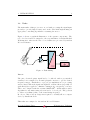
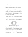
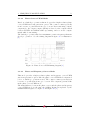
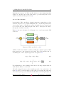
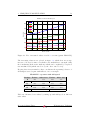
Figure 1 shows a graphical illustration of the system components. The
red colored sections were assigned to the responsibilities of student Michael
Weißensteiner, whereas the blue colored tasks were processed by student
Robert Viehauser.
Frequency
detection
Motor
µ C
Display / Control buttons
Programmable Gain
Amplifier
Guitar
Frequencymanipulation
Figure 1: Task sharing
Part 1:
The pure electrical guitar signal had to be filtered with a pre-switched
circuitry before sampled by an analog-digital-converter to get the desired
frequency ranges. Furthermore a proper pre-amplification for processing
was necessary. When the signal was digitized, software filters (especially biquad filters) were applied to eliminate existing noise or frequency overtones.
R
Those were designed with the software MATLAB
. Additionally a stable
algorithm for automatic string selection had to be developed. The goal was
to deliver a (realtime) value of the actual string frequency.
In order to that, a layout design was required to actually allow a compact
device by handicraft work.
This tasks were assigned to the student Robert Viehauser.
Motorized Guitar Tuner
Weißensteiner, Viehauser
1
INTRODUCTION
7
Part 2:
To actuate the motor a compatible PWM configuration had to be determined. Additionally, the motor had to be modified to allow a angular speed
controlled operation.
To obtain an accurate tuning procedure, a control system was designed by
R
using MATLAB
/Simulink. For this, researches about the guitar string
behaviour were necessary. Mathematical descriptions and conclusions were
made to create a control system model. Software supported simulating of
different PID-controller parameters provided a comfortable method for controller design.
In addition to that, a menu structure was required for selecting different
tuning modes and to access and edit tuning parameters.
This tasks were assigned to the student Michael Weißensteiner.
Motorized Guitar Tuner
Weißensteiner, Viehauser
2
FREQUENCY DETECTION
2
8
Frequency detection
2.1
2.1.1
Hardware
The µ-Controller[1]
The target of this project was to engineer a hand-held device and keeping
everything as simple as possible to build this device with limited funds. To
achieve this goal, a µ-Controller was chosen whose functionality is manageable and the appropriate circuit boards can be made by hand. This implies
that a PDIP packaging type with a pin distance of 100 mil (2.54 mm) was
preferred. Since we are in possession of a self made tiny USB programmer
R
R
for ATMEL
products and had some experiences with these, the ATMEL
Mega32 µ-Controller was chosen. For this project important features of the
µ-Controller are
• Up to 16MHz clock
• On-chip 2-cycle Multiplier
• Included 10-bit ADC1
• Build-in PWM2 -Module
• SPI3 module
• Programmable with our tiny USB programmer
2.1.2
Adaptive gain preamplifier
Before sampling the guitar signal with the implemented ADC of the µController is possible, some analog signal preprocessing stages are necessary.
The signal which comes straight out of a normal electric guitar has typically
20mV to 80mV peak to peak voltage. This also depends strongly on the
picked string. The thinner a guitar string is, the lower output voltage can
be measured, as a fact of the lower swinging metal volume which inducts the
tone as voltage signal in the pick-up of the guitar. Additionally the longer a
string swings, the lower amplitude the signal gets. This is obviously a fact
which has to be considered, since a sampling resolution as high as possible is
desired. To deal with this issue, it was decided to implement a programmable
gain stage.
1
Analog Digital Converter
Pulse Width Modulation
3
Serial Peripheral Interface
2
Motorized Guitar Tuner
Weißensteiner, Viehauser
2
FREQUENCY DETECTION
9
The preamplifier should be programmed by the µ-Controller itself. For this
R
purpose the MCP6S21 [2] from Microchip
is used, which also supports the
SPI protocol. This chip consists of an integrated non-inverting amplifier,
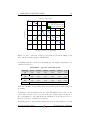
which can be programmed to one of 8 different gain levels.
1x
The supported gain levels are
2x 4x 5x 8x 10x 16x 32x
To achieve more and finer steps between two gain levels, two chips are driven
in cascade. With this trick and ensuring that each chip can be programmed
independently, the system is able to operate with the gain levels figured in
table 1, which are numbered in ascending order by the resulting gain of both
stages. This order defines the gain stage hierarchy used in the µ-Controller
program.
The gain step factor describes the multiplication factor that an increase of
one gain level (to the level in the corresponding row) implies. As this gain
step factor is about 1.25 in a wide spread connected range of gain levels, a
well controllable behavior of the whole preamplifier stage can be assumed,
since mostly an increase of one gain level means that the signal amplitude
increases up to 25%, which is quite good to handle.
This would be much more difficult with just one programmable amplifier chip
of this type. Additionally to finer gain increases, using two chips enables
the system to handle a bigger range of signal amplitudes too, which comes
together with a better handling of different guitars and guitar types.
Additionally to these programmable gain amplifiers a fixed gain stage is
introduced as well, to obtain a proper voltage level using the lower numbered
but well controllable gain stages assuming a signal starting at a level of
approximately 60mV peak to peak voltage. This achieves the possibility for
flexible and fine gain adjustments, which leads to an optimal exploitation of
the given ADC resolution during the whole tuning process.
These in sum three gain stages are also configured as active low- and highpasses. So an analog band-passing of the signal can be performed to avoid
direct components and aliasing due to the sampling. The electrical circuit of
the whole analog preprocessing is described in more detail in chapter 2.1.4
2.1.3
Single supply issues
Building a hand-held device often implies the usage of a battery which has
one minus and one plus pole. For processing the negative and positive parts
of the signal, the operational amplifiers need a positive supply voltage, a
negative supply voltage and an additional ground potential as reference. So
a virtual analog ground voltage whose electrical potential lies approximately
Motorized Guitar Tuner
Weißensteiner, Viehauser
2
FREQUENCY DETECTION
Level
Nr
0
1
2
3
4
5
6
7
8
9
10
11
12
13
14
15
16
17
18
19
20
Gain of
stage 1
1
1
2
1
2
2
4
4
5
4
5
5
8
8
10
8
10
8
10
16
32
Gain of
stage 2
1
2
2
5
4
5
4
5
5
8
8
10
8
10
10
16
16
32
32
32
32
Gain of
stage 1 × 2
1
2
4
5
8
10
16
20
25
32
40
50
64
80
100
128
160
256
320
512
1024
10
Gain step
factor
2
2
1.25
1.6
1.25
1.6
1.25
1.25
1.28
1.25
1.25
1.28
1.25
1.25
1.28
1.25
1.6
1.25
1.6
2
Resulting gain with
4.7x gain prestage
4.7
9.4
18.8
23.5
37.6
47
75.2
94
117.5
150.4
188
235
300.8
376
470
601.6
752
1203.2
1504
2406.4
4812.8
Table 1: Gain table of cascaded stages
in the middle of the plus and minus supply voltage of the battery has to
be generated. A simple method would be a 1-by-2 voltage divider, but its
output would not be able to stabilize its voltage under load, so a unity gain
buffer has to be added. Unfortunately our already ordered dual operational
amplifier LM358 [4] doesn’t support the usage as a unity gain buffer, so
a 1-by-11 voltage divider followed by a 5.7x non inverting gain stage was
used. This leads nearly to the same virtual ground voltage whose potential
is capable to be constant even under alternating load conditions.
Motorized Guitar Tuner
Weißensteiner, Viehauser
2
FREQUENCY DETECTION
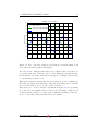
2.1.4
11
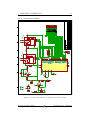
Connection scheme
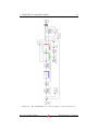
Figure 2: Connection scheme of the main electrical circuit
Motorized Guitar Tuner
Weißensteiner, Viehauser
2
FREQUENCY DETECTION
12
Figure 2 shows the electrical connection scheme of the main circuit. The
virtual analog ground voltage which was mentioned above is generated in
region B1 of the scheme. This voltage is used as reference for the guitar signal
and for the all following gain stages shown in region A2 to A4. The absolute
resistor values of the 1-by-11 voltage divider (R1 and R2) are chosen as a
tradeoff between noise immunity and low current flow. If the resistor values
are chosen too high, the thermal resistor noise will influence the stability
of the reference voltage. Choosing too low resistor values would cause a
high current which effects the lifetime of the battery in a negative way. The
capacitor C1 is supposed to improve stability of the reference voltage in case
of fluctuation of the supply voltage.
The non inverting gain stage will keep the output reference voltage constant,
even under load. The gain can be calculated according to following equation
1.
R3
4, 7kΩ
Gref = 1 +
=1+
= 5, 7
(1)
R4
1kΩ
Assuming a supply voltage of Usup = 5V leads to a virtual ground voltage
of
1
1
Usup ·
· Gref = 5V ·
· 5, 7 = 2, 59V
(2)
11
11
which is a satisfying reference voltage for this purpose.
The active low-pass with a fixed gain of 4.7x is represented in section A2.
As input signal the guitar signal is directly connected by connector CONN2,
which is also referenced by the virtual ground voltage. The cutoff frequency
and the gain of the first stage can be calculated as shown in equation 3 and
4.
1
1
fcLP 1 =
=
= 497, 98Hz
(3)
2π · C2 · R6
2π · 6, 8nF · 47kΩ
Gf ix = −
R6
47kΩ
=−
= −4, 7
R5
10kΩ
(4)
As first gain stage an inverting amplifier circuit is used. This setup is much
more resistant to noise than a non inverting amplifier, because the input
resistance of a non inverting circuit is very high (theoretically infinite). The
input resistance of a inverting amplifier circuit is approximately the value
of the resistor between the input signal source and the inverting input of
the operational amplifier (in figure 2 labeled as R5). The thermal noise of a
resistor is directly related to its value, so a lower resistor inducts less noise.
The value 10kΩ for R5 was chosen as a tradeoff of low thermal noise and
keeping the load to the signal source small. If choosing the value for R5 too
low (high load), the voltage amplitude of the guitar signal will collapse.
Since just the frequency is interesting when tuning a string, the negative
sign (and the whole phase response) is not relevant in this application.
Motorized Guitar Tuner
Weißensteiner, Viehauser
2
FREQUENCY DETECTION
13
The programmable gain stages shown in figure 2 (regions A3-A4) consist
internally of non inverting gain stages. To drive them as active gain stages
with low- and high-pass characteristics, the input signal of each stage is filtered through simple passive elements. The high-pass consists of C3 and R7,
the second low-pass consists of C4 and R8.
fcHP =
1
1
=
= 21, 92Hz
2π · C3 · R7
2π · 330nF · 22kΩ
(5)
fcLP 2 =
1
1
=
= 408, 09Hz
2π · C4 · R8
2π · 39nF · 10kΩ
(6)
There are several reasons for this configuration of the gain stages. The highpass stage is responsible for eliminating a possible direct component of the
signal without influencing the interesting frequency components (the lowest
target frequency of the system is the low D at 73, 42Hz, see table 2 in section
2.2.2). The two low-pass stages are responsible for avoiding aliasing caused
by sampling the signal after the preamplifier stage. Also the amplitudes of
harmonic frequencies get reduced while the interesting fundamental frequencies are not influenced (the highest target frequency the system is designed
for is the high E at 329, 63Hz, also shown table 2 in section 2.2.2). Two
cascaded low-pass stages cause a second order low-pass characteristic above
the higher cut-off frequency (497, 98Hz), so the harmonic components are
much more suppressed as one low-pass stage would be able to.
The single frequency characteristics of the three stages don’t interact with
each other like pure passive networks would, because they are decoupled by
the operational amplifiers.
The amplified and pre-filtered signal is directly connected to the input of the
internal ADC of the µ-Controller (ADC0 pin). Since the whole preprocessing
components are referenced on the virtual ground voltage (≈ 2, 5V ) and the
µ-Controller is able to sample values between 0V and 5V , no additional decoupling is needed to measure the positive and negative alternations of the
signal.
To enable data transfer, the programmable gain stages are connected to the
MOSI4 and the SCK5 port of the µ-Controller. With additional independent
chip select connections to each programmable amplifier (CS → PB3 and PB4
), the µ-Controller is able to program the gain stages separately. For more
information on this procedure see section 2.3.1.
Connector CONN3 provides the ISP-Interface6 for the µ-Controller and is used
for updating and maintaining the software running on the chip without the
need of disassembling. Due to the ISP-Interface uses the SPI protocol, some
4
master-out-slave-in
slave clock
6
ISP = In-System-Programming
5
Motorized Guitar Tuner
Weißensteiner, Viehauser
2
FREQUENCY DETECTION
14
pins are connected to the same ports as the programmable gain amplifiers.
Connector CONN4 connects the hardware components of the interface with
the main board and CONN5 supplies the servo motor with power and command instructions (OC1B) from the µ-Controller.
Due to the high inrush current of the servo motor, the capacitor C6 is needed
to stabilize the supply voltage of the whole circuit. The 16M Hz oscillating crystal is connected to its supposed ports XTAL1 and XTAL2 and C5 is
recommended to help the internal ADC to stabilize its reference voltage.
Motorized Guitar Tuner
Weißensteiner, Viehauser
2
FREQUENCY DETECTION
2.2
15
Pitch detection theory
There are many possible approaches to detect the pitch of the signal. In
music theory the pitch is the subjective frequency like property of a tone,
which is assigned by the human sense of hearing. Pitch and frequency are
strongly related, but they are not equivalent. Whereas the pitch is a subjective opinion to categorize a tone, the frequency is a objective scientific
property of a signal expressed by a value and its unit. In the following
discussed approach(es) to detect the pitch, the pitch and the fundamental
frequency of the sampled signal are assumed as equivalent. This assumption
should lead to satisfying results even for trained musicians.
2.2.1
A resource saving frequency unit
Usually the unit of the frequency (in this application also the control parameter) is Hz. Its value is mostly determined by the inverse of the periodic
time which is delivered by any chosen method. To calculate the periodic
time within a discrete working system driven by a clock, also a division of
a certain number of values between one period by the sample rate becomes
necessary.
Additionally after determining the discrete values which represent the beginning and the end of a period, maybe some interpolation and averaging is
needed to gain more accuracy.
All these calculations (interpolation, averaging, dividing by the sampling
rate, calculating the inverse) costs additional time and are just transformations from a discrete number of samples to the well known unit Hz.
Since calculation resources are limited anyway, a new system-wide unit for
the frequency, more precisely the periodic time was introduced: the number of samples within 4 periods. Hence, dividing by the sample rate and
calculating the inverse become not needed anymore. This arrangement also
makes interpolation unnecessary, since when speaking of one period the time
between two samples divided by 4 can be distinguished. This trick has also
the same effect like averaging 4 values (but without the dividing operation),
so an accuracy which is high enough for the tuning process without the need
to handle with decimal places is achieved.
Motorized Guitar Tuner
Weißensteiner, Viehauser
2
FREQUENCY DETECTION
2.2.2
16
Time and accuracy tradeoff
Before the different pitch detection methods are described, it has to be mentioned that special care has to be taken of running out of memory resources.
A higher sampling rate means more accuracy, but also comes with more
data to process. The chosen µ-Controller features an internal RAM of 2kB,
whose usage has to be well-considered.
Because a control system has to be implemented, the time an update of
the frequency information takes, is also an critical parameter. A tradeoff
decision between accuracy, memory and speed has to be made.
The number of samples within 4 periods is an applicable control parameter
for all further discussed methods to detect the pitch. Due to the minimal
limit of the sampling rate (which is needed to provide accuracy without interpolating) and the necessary calculating time of a chosen method added
to the time the controlling needs is too extensive to be finished in the time
between two samples, it was decided to build a cycle of a measuring and a
controlling task. The first task performs the recording of a part of the signal with simultaneously gaining the pitch information and the second one is
doing the frequency tuning when the pitch is completely determined. After
that, new samples are recorded and the cycle continues.
As a tradeoff of time, memory resources and accuracy a sampling rate of
8kHz was chosen. With this sampling rate a number of about 1000 samples can be recorded to gain the frequency information also comes with
still having enough memory for other required tasks. For the three tuning modes which should be implemented (standard tuning, drop-d tuning,
one-step-down tuning) 12 target notes are necessary. Table 2 shows these
target notes together with their defined physical frequencies, the number of
samples within 4 periods (@ a sampling rate of 8kHz) and the error due to
the representation in the introduced unit. The frequency values were taken
from reference [5].
The gray marked rows are the notes which are used in one-step-down tuning, where notations on white background representing the standard tuning.
Drop-D tuning consists of a low D tuned first string and standard tuning of
the other five strings.
The representation error is shown in Hz and in cent. Cent is a unit which
tries to model the human sense of hearing. The number of cents between
two different tones which a human is able to distinguish, varies from human
to human. According to the most people humans can distinguish 5−6 cents,
but for tuning a guitar an error of 5 − 6 cents should be quite satisfying. As
you can see in table 2 the representation of the frequency information in the
Motorized Guitar Tuner
Weißensteiner, Viehauser
2
FREQUENCY DETECTION
English
notation
high E
high D
B (ger: H)
A
G
F
D
C
A
G
low E
low D
Frequency
[Hz]
329.628
293.665
246.942
220
195.998
174.614
146.832
130.813
110
97.9989
82.4069
73.4162
# samples within
4 periods @ 8kHz
97
109
130
145
163
183
218
245
291
327
388
436
17
Representation
error [Hz / cent]
0.269 / 1.412
0.087 / 0.513
0.788 / 5.517
0.690 / 5.419
0.321 / 2.833
0.249 / 2.471
0.043 / 0.507
0.201 / 2.655
0.034 / 0.541
0.140 / 2.464
0.067 / 1.414
0.022 / 0.512
Table 2: Table of all target notes
introduced unit should lead to very good results, because the error caused
by this representation measured in cents is pretty low.
2.2.3
The signal
Since only the frequency information has to be extracted out of the signal
and due to memory issues, it was decided to use just 8-bit values to represent
the signal.
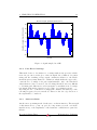
Figure 3 shows the recorded signal like it is sampled by the µ-Controller. To
simulate different methods as realistic as possible, different guitars connected
to the MIC input of the PC were recorded at a sampling rate of 8kHz, folR
lowed by an amplitude quantization down to 8 bit using MATLAB
. About
12 different test signals of 4 different guitars were taken as a good base to
develop a practicable pitch detection method. Figure 3 shows the oscillation
of a correctly tuned low E string. It is clear to see, that the guitar signal
doesn’t consist of just a single sine wave.
Many methods to detect the pitch of the guitar signal try to gain the frequency information by determining an oscillation whose frequency is equal
to the frequency of the fundamental oscillation and extracting the number
of samples within one period by detecting zero crossings. Some methods to
determine this oscillation are described in the following sections.
Motorized Guitar Tuner
Weißensteiner, Viehauser
2
FREQUENCY DETECTION
18
Measured signal, quantized and discretized
Amplitude in signed integer 8 bit resolution
60
40
20
0
−20
−40
−60
−80
1
1.005
1.01
1.015
1.02
1.025
Seconds
Figure 3: Signal sampled at 8kHz
2.2.4
Pure Zero Crossings
This method tries to determine zero crossings without any previous calculations. As you can see in the plot of the test signal, the oscillation of a guitar
string and the resulting voltage signal contains in addition to the fundamental frequency many harmonic oscillations, which makes the approach to
count the zero crossings of the pure signal unusable. Also other threshold
values than zero have been tried, but a working threshold was very difficult
to determine and different for each test signal, even within areas of a single
test signal. This method was rejected because of robustness reasons.
Detecting the zero or threshold crossings will constitute the final step of the
following frequency detection methods. Therefore also the edge direction of
the signal will be considered.
2.2.5
Autocorrelation
Another more promising method is the autocorrelation function. The strength
of this function is to point out periodic components very well, even if the
signal is noisy or the amplitudes of the harmonic oscillations are quite distinctive.
Motorized Guitar Tuner
Weißensteiner, Viehauser
2
FREQUENCY DETECTION
19
The formula to calculate the autocorrelation function is
N −1
1 X
xn · xn−τ
Rxx (τ ) = lim
N →∞ N
n=0
where xn is the recorded signal and N is the length of the signal. Since
the system operates with discrete finite signals, a condition for the signal
boundaries has to be defined. In this application xn = 0 : n < 0, n > N − 1
was chosen, because enough samples are taken and this constraint prohibits
from additional calculation effort, which would require more resources.
Amplitude in 8 bit signed integer
ACF calculation using the measured signal, tau = 2 samples
100
50
0
−50
−100
1
1.005
1.01
1.015
Seconds
1.02
1.025
Amplitude in 8 bit signed integer
ACF calculation using the measured signal, tau = 6 samples
100
50
0
−50
−100
1
1.005
1.01
1.015
Seconds
1.02
1.025
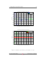
Figure 4: Illustration ACF-calculation
Figure 4 shows a graphical demonstration how to calculate the ACF (autocorrelation function) Rxx (τ ) for 2 values (τ = 2; τ = 6). To generate this
plot, the signal of figure 3 was used as input signal. To calculate one value of
the ACF, all overlapping values of the green function and the blue function
shifted by τ are point-wise multiplied and accumulated. The sum is then
Motorized Guitar Tuner
Weißensteiner, Viehauser
2
FREQUENCY DETECTION
20
divided by the number of samples to normalize the result. In this illustration the whole signal consists of about two periods, in practice the number
of samples is much higher (like about one thousand samples as mentioned
before).
Unfortunately the calculation task of the ACF is very tough for the calculation capability of the chosen µ-Controller and each value of the autocorrelation function depends on the whole signal, that means before the first data
point of the ACF can be determined, the recording of the full signal must be
finished. This circumstance would lead to a long frequency detection delay,
which would be very difficult to handle for the controlling task.
Hence an approach which uses just a part of the signal for one value of the
autocorrelation function was developed. Much less calculations are needed
when only a small amount of samples is used to “slide” over the whole
signal. This so called partial autocorrelation function should also fulfill the
same characteristics of the full autocorrelation function. Of course this small
amount of samples should be at least greater than the samples within one
period. When a lowest frequency to detect of about 70Hz is assumed, the
number of samples to represent one period at a sample rate of 8kHz is
sample rate
8000Hz
=
≈ 114 samples
frequency
70Hz
So a sliding signal of 120 samples was chosen. This signal always covers areas
where the full signal is defined. Hence, no boundary condition is necessary.
Assuming the length of the sliding signal is L, when starting at τ = 0 (where
the first value of the sliding part of the signal overlaps with the first value of
the full signal) and ending at τ = N − L (where the last value of the sliding
signal values overlaps with the last value of the full signal), we get a partial
autocorrelation function which consists of N − L + 1 values.
This method can also be interpreted as a cross correlation of a part of
the signal with the signal itself. Using just a part of the signal for one
multiplicand, changes the formula of the autocorrelation as follows
Rxp x (τ ) =
L−1+τ
1 X
xn · xn−τ
L n=τ
0≤τ ≤N −L
where x is the full recorded signal, xn−τ indexes the sliding part of the signal,
L indicates its length (120 samples) and N is the length of x.
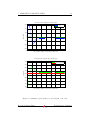
Figure 5 shows a illustration how this approach works. In practical application the full signal (the green colored values) consists of much more values
than the sliding part of the signal (about 9 times).
Motorized Guitar Tuner
Weißensteiner, Viehauser
2
FREQUENCY DETECTION
21
Amplitude in 8 bit signed integer
PACF calculation using the measured signal, tau = 2 samples
100
50
0
−50
−100
1
1.005
1.01
1.015
Seconds
1.02
1.025
Amplitude in 8 bit signed integer
PACF calculation using the measured signal, tau = 50 samples
100
50
0
−50
−100
1
1.005
1.01
1.015
Seconds
1.02
1.025
Amplitude in 8 bit signed integer
PACF calculation using the measured signal, tau = 100 samples
100
50
0
−50
−100
1
1.005
1.01
1.015
Seconds
1.02
1.025
Figure 5: Partial ACF-calculation
Motorized Guitar Tuner
Weißensteiner, Viehauser
2
FREQUENCY DETECTION
22
The big advantages gained by using this method are a much less number of
multiplications to compute and the ability to calculate values of the PACF
function even if the signal isn’t completely recorded. This leads to much
more efficient usage of time, memory and processing resources.
Table 3 illustrates how values of the PACF function can be calculated, even
if the recording process hasn’t been finished.
Assuming a sliding signal size of L = 5 samples, the first value of the PACF
(Rxp x (0)) equals the sum of the products of x0..4 and x0..4 , (n = 0..4).
After the first L samples, the calculation of Rxp x (0) is done. The next
value Rxp x (1) is calculated by summing up the products of x0..4 and x1..5
(n = 1..5), and so on.
To use the time resources as efficient as possible, the calculation of the required products can be performed during the waiting periods between two
samples. When the first value is sampled, it can be multiplied by itself.
Since each product is just needed once, it’s unnecessary to save them. The
first product is stored in an cleared accumulator variable of a size of 32-bit
(to prevent overflow effects). When the second value is sampled, two products which are necessary for the PACF value can be calculated. x1 times
x1 will be added to the first accumulator variable, and x0 times x1 will be
the content of a second accumulator variable. When the third value is sampled, 3 products can be determined and so forth. Due to this procedure
the time resources are used optimally. When L values are sampled, the first
accumulator variable contains the result of Rxp x (0). After checking for zero
crossings, this result becomes unimportant and the variable is free for reset
and reuse. Hence just L accumulator variables are needed for the whole
algorithm, so this method is quite memory resources saving.
The procedure of sampling the signal and calculating the PACF simultaneously leads to following pseudo code:
PACF[0..L-1] = 0 //accumulator variable array
for n = 0:N-1
x[n] = getNextValue()
for i = 0:min(n,L-1)
idx = (n - i) mod L
PACF[idx] += x[i]*x[n]
end
if n >= L-1
checkForZeroCrossing(PACF[idx])
PACF[idx] = 0
end
end
Motorized Guitar Tuner
Weißensteiner, Viehauser
2
FREQUENCY DETECTION
23
n
x
0
0
x
1
2
n−τ
3
4
:
L−1
1
2
3
4
5
6
7
8 ... N − 1
o x o x o x o x
o
o x o x o x o x
o
x o x o x o x
o
o x o x o x
o
x o x o x
o
Rxp x (0) (1) (2) (3) (4) .. (N − L)
Table 3: Calculation table of the optimized PACF
To save additional processing resources, it was passed on normalizing the
resulting PACF, because we are just interested on detecting zero crossings.
5
PACF
x 10
1.5
Amplitude
1
0.5
0
−0.5
−1
1
1.01
1.02
1.03
1.04
Seconds
1.05
1.06
1.07
Figure 6: Resulting partial autocorrelation function
Performing the described calculations on a tuned low e string (see figure 3)
leads to the function which is shown in figure 6. (This function representing
the PACF is still a discrete function, it is just plotted as connected line
diagram to illustrate the threshold crossings described underneath.) The
test signal was contaminated by white Gaussian noise with a signal to noise
ratio (SNR) of 40dB.
Motorized Guitar Tuner
Weißensteiner, Viehauser
2
FREQUENCY DETECTION
24
It is clear to see, that there are still harmonic components indicated by
a lower amplitude in the function. So detecting the zero crossings would
lead to wrong frequency results. The pitch of the signal is represented by
significant higher amplitudes. So a threshold whose value is proportional to
the highest value of the PACF is used. The pitch is detected by the threshold
crossings with respect to the edge of the PACF. Because the amplitude of
the pure signal is not expected to change within 4 periods, the maximum of
the PACF is assumed to equal the first value of Rxp x (τ ) at τ = 0. At this
point the signal is correlated by itself and is expected to cause the highest
value for the correlation function.
Different trials showed, that a threshold whose value equals 85% of the first
value gives the most robust results.
In figure 6 the threshold is represented by the dotted black line and its
crossings are indicated by vertical colored lines. Since the calculation of the
PACF is canceled when its value crosses the threshold the fifth time, the last
ridge which crosses the threshold looks lower than the others. Continuing the
calculation of the PACF would cause a similar ridge as those which occur
after the first four threshold crossings. Canceling the calculation doesn’t
effect the result, because the checking for threshold crossings is executed for
finished values only. That means, that in figure 6 the first value after the
fifth threshold crossing is the last finished one, the subsequent values equal
the unfinished accumulator states.
Although this method looks quite robust and the calculation effort is reduced
to a minimum, there is a more efficient and accurate method to calculate the
pitch of the signal. Due to the harmonic components which are still included
in the PACF, the resulting frequency information can be influenced by these
components and can cause critical inaccuracy.
2.2.6
Digital Filters
The autocorrelation points out periodic components of the input signal by
analyzing the unchanged measured values. The approach to use digital filters
tries to manipulate the signal in a way, that there is just the fundamental
frequency left. After that filtering, a zero crossing detection should lead to
the pitch information.
There exist many types of digital filters. The two major groups are finite impulse response filters (FIR-filters) and infinite impulse response filters (IIR).
The result of a FIR filter is calculated by a linear combination of a finite
number N of past input values, whereas IIR filters also take past output
values into account. FIR filters require usually much more multiplication
and storage elements to determine the filtered signal. N is also called the
order these filters. The filter operation of a FIR filter can be mathemati-
Motorized Guitar Tuner
Weißensteiner, Viehauser
2
FREQUENCY DETECTION
25
cally described using equations 7 and 8, where x is the input signal, y is the
output signal and bk are the filter coefficients.
y[n] = b0 x[n] + b1 x[n − 1] + b2 x[n − 2] + ... + bN x[n − N ]
=
N
X
bk x[n − k]
(7)
(8)
k=0
Represented as block diagram, a FIR filter looks like shown in figure 7.
The memory elements are shown as z −1 , due to the representation of delay
elements after the z-transformation.
x[n]
z-1
z-1
z-1
b_0
b_1
b_2
+
+
z-1
b_3
+
+
b_N
+
+
+
y[n]
+
Figure 7: Block diagram of a FIR-filter
To design useful filters for this application, a FIR filter would need too
much multiplication and storage resources. The advantage of FIR filters is
that the calculation task can be massively parallelized if there are enough
calculation units available like in a digital signal processor (DSP).
In case of a single core processing unit like the ATMEGA 32, it is much
more efficient to use an IIR filter. The output function of this type of filter
can be mathematically described as follows (9). In addition to the FIR filter
the output filter coefficients ak are introduced.
y[n] = − a1 y[n − 1] − a2 y[n − 2] − ... − aN y[n − N ]
+ b0 x[n] + b1 x[n − 1] + b2 x[n − 2] + ... + bN x[n − N ]
(9)
Again, N defines the order of the IIR filter. To design similar filter characteristics as known FIR filters, the order of the IIR filters can be much lower.
This is the advantage of IIR filters for systems with limited resources. An
IIR filter with order N = 2 is called “biquad filter”, which is already a very
powerful construct. Equation 10 describes the calculation for a biquad filter,
which is quite simple.
y[n] = −a1 y[n − 1] − a2 y[n − 2] + b0 x[n] + b1 x[n − 1] + b2 x[n − 2]
(10)
This formula can be illustrated as a block diagram in the z-domain too,
shown in figure 8. This form is called the direct form 1.
Motorized Guitar Tuner
Weißensteiner, Viehauser
2
FREQUENCY DETECTION
26
b0
y[n]
x[n]
+
+
+
+
z-1
z-1
b1
-a1
+
+
+
+
z-1
z-1
b2
-a2
Figure 8: Block diagram of a biquad filter: direct form 1
b0
x[n]
y[n]
+
+
+
+
z-1
z-1
b1
-a1
+
+
+
+
z-1
-a2
z-1
b2
Figure 9: Block diagram of a biquad filter: switched stages
The block diagram can be seen as a transfer function in the z-domain which
consist of two parts. The part which determines the linear combination of
the input values and the bk coefficients, is called HB (z). The other part is
called HA (z), respectively. According to the commutative law for Z-transfer
functions (H(z) = HB (z) · HA (z) = HA (z) · HB (z)), the parts of the block
diagrams can be switched which leads to the illustration showed in figure 9.
Now it is clear to see, that the horizontal neighbored memory blocks contain
always the same value. So these blocks can be replaced by one, shown in
figure 10. This constellation of the elements in the block diagram is called
direct form 2.
To save additional memory resources, biquad filters of the direct form 2 are
used in this application.
As powerful and flexible the biquad filters are, their magnitude response
is too flat to extract the fundamental frequency of a guitar string oscillation and simultaneously suppress the harmonic components completely. In
Motorized Guitar Tuner
Weißensteiner, Viehauser
2
FREQUENCY DETECTION
27
b0
y[n]
x[n]
+
+
+
+
z-1
-a1
b1
+
+
+
+
z-1
-a2
b2
Figure 10: Block diagram of a biquad filter: direct form 2
respect to the 8 bit signed integer representation of the measured values
(−128 to 127), a harmonic component suppression of about −40dB is desired. To achieve this constraint, higher ordered digital filters or a cascade
of biquad filters can be used. Since the filters have to be implemented on
a 8-bit architecture, it was decided to use cascaded biquad filters, because
these constructs are much more immune to stability issues than higher ordered filters. Figure 11 shows the so called second-order-sections filter (SOS
filter), which consists of a cascade of two biquad filters.
b0
x[n]
+
b’0
x’[n]
+
+
+
+
+
z-1
-a1
z-1
b1
+
-a’1
+
b’1
+
+
+
+
+
+
z-1
-a2
y[n]
+
+
z-1
b2
-a’2
b’2
Figure 11: Block diagram of a second-order-section filter
After deciding which filter architecture is applied, the different filters can
be designed. To extract the fundamental frequency for the different target
frequencies as accurate as possible, for each target frequency one specialized
filter is needed. These filters are supposed to suppress the harmonic components about 40dB at least and have their maximum magnitude responses
at the corresponding target frequencies. The major problem of such specialized filters is the difficulty to detect frequencies which are not in the small
frequency band around the target frequencies. To ensure this functionality,
also some generalized filters are necessary. The decision was made, that one
Motorized Guitar Tuner
Weißensteiner, Viehauser
2
FREQUENCY DETECTION
28
generalized filter should cover the expected frequency range of one string. To
choose the best filter for the actual fundamental frequency, filter boundaries
are defined. If the current detected frequency crosses such a boundary, the
recorded values of the next cycle are processed with the filter corresponding
to that next frequency band.
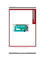
Figure 12 shows a screenshot of the filter design and analysis tool (“fdaR
tool”) of MATLAB
. Aided by this tool, 12 specialized and 6 generalized
second-order-section filters have been designed.
R
Figure 12: Designing the SOS-filters using “fdatool” in MATLAB
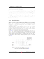
The magnitude responses of the designed filters are illustrated in figure 13.
The black dashed lines represent the generalized filters, the blue lines indicate the specialized filters for the standard tuning and the magenta lines
extended with the yellow line show the magnitude response for the specialized filters for the one-step-down tuning. For drop-D tuning the yellow
drawn filter and the five most right aligned blue lined filters are used. The
threshold boundaries between the generalized filters were defined at their
crossing points and the boundaries of the specialized filters were defined at
their undercut of the −3dB threshold.
Motorized Guitar Tuner
Weißensteiner, Viehauser
2
FREQUENCY DETECTION
29
Magnitude Response
0
−5
Magnitude (dB)
−10
−15
−20
−25
−30
−35
−40
−45
−50
0
0.05
0.1
0.15
0.2
0.25
0.3
Frequency (kHz)
0.35
0.4
0.45
0.5
Figure 13: Magnitude response of used filter bank
2.2.6.1 Representation of numbers A critical issue of working with
IIR filters is always the stability. Their filter coefficients consist usually of
numbers with many decimal places. The designed filters can become unstable easily, if too much rounding errors are made. Due to the missing
floating point functionality of the µ-Controller, special care has to be taken
to the representation of numbers. To be able to represent numbers between
0 and 1, a fixed decimal point is introduced. This is a common method to
represent decimal numbers, when digits are limited.
For example in a binary numbering system of 8 bit, the usual number representation looks like shown in table 4. The highest (unsigned) number which
can be represented is 255 (sum of the worth row).
If a 2 bit fix point representation is defined per convention, the worth of
each bit equals the values shown table 5. The highest number which can
be represented now decreases to 63.75, but a decimal resolution of 0.25 is
achieved.
bit number
worth
7
27
128
6
26
64
5
25
32
4
24
16
3
23
8
2
22
4
1
21
2
0
20
1
Table 4: Standard 8 bit number representation
The chosen µ-Controller can handle a maximum of 32 bit per variable. First
of all a decimal point after the 16th digit was introduced. This enables to
Motorized Guitar Tuner
Weißensteiner, Viehauser
2
FREQUENCY DETECTION
bit number
worth
7
25
32
6
24
16
30
5
23
8
4
22
4
3
21
2
2
20
1
1
2−1
0.5
0
2−2
0.25
Table 5: 8 bit number representation using 2 bits as decimal digits
distinguish values with a resolution of
1
2−16 = 16 ≈ 0.00001526,
2
which is small enough to ensure stability of the filters. Unfortunately choosing the 16th digit to represent “1” implies, that there are just 16 bits left to
represent higher numbers. So choosing the 16th digit reduces the range of
32 bit signed integer numbers from
−231 ... 231 − 1 = −2.147.483.648 ... 2.147.483.647
to
−216 ... 216 − 1 = −65.536 ... 65.535.
This smaller range seems to be sufficient for the coefficients and the filtered
signal values, but not for the multiplication operation. Assuming a convention of 2 binary decimal places like in table 5, an integer number can be
transformed from the standard convention as shown in table 4 to this new
numbering format by shifting its binary value 2 digits to the left. In a binary system this equals a multiplication operation with 4 (22 ). To perform
a multiplication of two values in this fixed decimal point representation, the
result was implicitly multiplied by 22 · 22 = 16. Hence the result has to
be shifted back to the right by the defined number of decimal digits. So
even if the result of the multiplication fits in this range, the intermediate
result before the right shift operation may not. Indeed, some intermediate
calculation results exceed this range when placing the virtual decimal point
after the 16th digit, which causes again instability as a result of bit overflow.
Simulations showed, that these intermediate calculations require often 20
bits to represent the result in binary representation. So the decimal point
was placed after the 20th bit. The number of remaining bits (32 − 20 = 12)
leads to a resolution of
1
2−12 = 12 ≈ 0.0002441
2
which is still small enough to save stability, if the filter coefficients of the
cascaded filters vary at least a certain value. This is the reason for some
specialized filters represented in figure 13 covering a wider frequency band
than others. Defining the decimal point after the 20th bit leads to a range
for signed integer values of
−220 ... 220 − 1 = −1.048.576 ... 1.048.575.
Motorized Guitar Tuner
Weißensteiner, Viehauser
2
FREQUENCY DETECTION
31
2.2.6.2 Evaluation of the filtered signal After providing the 12 bit
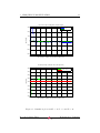
fixed-point convention to be able to calculate the filtered output signal,
the result has to be evaluated. Figure 14 shows the filtered signal of the
R
MATLAB
simulation calculated according to figure 11, using the filter coefficients of the specialized filter for the low E string. To generate this plot,
the same input signal (tuned low E) of the demonstration of the PACF (figure 6) was used. As done in figure 6, the signal is plotted as connected line
diagram to point out the shape of the output signal, but it still consists of
discrete values. To model the the limited capacities of the µ-Controller, also
the 12 bit fixed-point representation was implemented in the simulation. In
figure 14 the whole plot was clipped to the range of about one recording
cycle consisting of 1000 values.
As the filters are designed to suppress all harmonic components, detecting
the zero crossings will offer the frequency information of the fundamental
oscillation. Due to the introduced system-wide periodic time unit, just the
number of samples between 5 zero crossings has to be determined.
Before every recording cycle, the storage elements of the SOS filter have to
be reset to zero. Hence the filter needs some samples to establish the full
amplitude in each cycle. Due to this and possible additional information
delay, only the samples between the last 5 determined zero crossings are
taken into account. In this implementation the falling edge is considered,
but there is no special reason for that. The rising edge could be used as
well.
In the example shown in figure 14 the detected samples within 4 periods
would be 97 + 97 + 97 + 98 = 389, so the string is tuned slightly too low
(should be 388, according to table 2).
Figure 15 shows the same signal as plotted in figure 14 filtered by the generalized filter for the first string. The rough and non sinusoidal establishment
of the full amplitude and the variance of the number of samples between two
zero crossings of the falling edge indicate, that there are still harmonic components in the signal. This is quite plausible when looking at the magnitude
response of the filter (see figure 13). Determining the frequency information
would retrieve 97 + 97 + 97 + 96 = 387, a slightly hearable varying result as
above. Hence, the introduction of specialized filters is quite advantageous
and reasonable.
Figure 16 shows the filtered signal of a D string filtered by the specialized
filter for standard D. The number of samples within two zero crossings is
varying between 54 and 55, but is mostly 55. This depends on the discretization. When a value was sampled right after the afterwards detected
zero crossing, there is more change that the 55th sample also falls into this
period. Statistically the number of samples in one period of 54 and 55 have
Motorized Guitar Tuner
Weißensteiner, Viehauser
2
FREQUENCY DETECTION
5
1.5
32
Filtered signal
x 10
amplitude (in fix point respresentation)
1
0.5
0
54
97
98
98
97
98
97
1.06
seconds
1.08
97
97
98
35
−0.5
−1
−1.5
1
1.02
1.04
1.1
1.12
Figure 14: Evaluation of the filtered signal
5
Filtered signal
x 10
1
amplitude (in fix point respresentation)
0.8
0.6
0.4
0.2
0
55
−0.2
104
99
97
96
98
97
97
97
96
34
−0.4
−0.6
−0.8
−1
1
1.02
1.04
1.06
seconds
1.08
1.1
1.12
Figure 15: Evaluation of the filtered signal
Motorized Guitar Tuner
Weißensteiner, Viehauser
2
FREQUENCY DETECTION
33
to be equal when sampling a correctly tuned D string. (As you can see in
table 2, the number of samples within 4 periods should be 218 on a tuned
string. To get this value when evaluating the samples between 5 zero crossings, there has to be 55 + 54 + 55 + 54 = 218 or a similar constellation.)
In figure 16 there would be determined 55 + 55 + 55 + 54 = 219 samples as
frequency information, which indicated that the string is tuned also slightly
too low. This minimal divergence is pointed out by the introduced unit,
because counting the number of samples within 4 periods implies an average determination. This example shows how sensible the introduced unit is,
even without decimal places.
4
Filtered signal
x 10
amplitude (in fix point respresentation)
1
0.5
0
−0.5
−1
16 47 54 55 54 55 55 54 55 55 54 55 55 54 55 55 55 54 55 31
1
1.02
1.04
1.06
seconds
1.08
1.1
1.12
Figure 16: Evaluation of the filtered signal
2.2.6.3 String detection method for digital filters The major disadvantage of digital filters compared to the (partial) autocorrelation function
is that there has to be some information about the frequency before starting
the calculation. Without this additional information, the wrong filter could
be chosen which leads to extracting a harmonic component of the signal
instead of the fundamental frequency.
An approach which would work pretty sure, is to detect the first frequency
information using the autocorrelation function the first time. But it was
decided, that this approach would lead to unnecessary high effort for distinguishing between only six frequency intervals. Hence a method to select
the first generalized filter was developed which takes advantage of the high
Motorized Guitar Tuner
Weißensteiner, Viehauser
2
FREQUENCY DETECTION
34
quantity of taken samples. As the analysis process of the partial autocorrelation, the number samples between threshold crossings are evaluated. But
unlike the approach using the autocorrelation function, the unprocessed input signal is evaluated.
To manage the quantity of the expected threshold crossings, a voting scheme
was introduced. Each voting bin corresponds to one string. To evaluate a
vote, the number of samples between each fifth threshold crossing is counted.
Therefore the borders of the generalized filters can be used as voting bin borders. For instance if the counted number of samples lies between the two
borders of the generalized filter of the fourth string, the voting bin of the
fourth string is incremented by 1.
85% of the biggest value of the input signal is used as threshold. After
evaluating all numbers of samples between every firth threshold crossing,
the temporary detected frequency is set to the mean of the standard and
the one-step-down target frequency of the string which got the most votes.
So the filter choosing algorithm will use the generalized filter for the string
which got the most votes.
Figure 17 shows the voting result of 4 different strings tuned correctly in
standard tuning. For this simulation a Gaussian white noise with a signal
to noise ratio (SNR) of 40dB was added.
Figure 18 shows the voting result of the same 4 input signals of figure 17
without the white Gaussian noise. All strings, noisy or not, were determined
correctly, so this simulation indicates that the introduced voting scheme is
a well working and resource saving method to choose the first generalized
filter.
Motorized Guitar Tuner
Weißensteiner, Viehauser
2
FREQUENCY DETECTION
35
Result of string voting
14
25
12
10
20
number of votes
number of votes
Result of string voting
30
15
10
8
6
4
5
0
2
1
2
3
4
string number
5
0
6
(a) Voting result for the low E string
1
2
5
6
(b) Voting result for the D string
Result of string voting
Result of string voting
30
35
25
30
25
20
number of votes
number of votes
3
4
string number
15
10
20
15
10
5
0
5
1
2
3
4
string number
5
6
(c) Voting result for the high E string
0
1
2
3
4
string number
5
6
(d) Voting result for the G string
Figure 17: Voting results of different strings with white Gaussian noise of
40dB SNR
Motorized Guitar Tuner
Weißensteiner, Viehauser
2
FREQUENCY DETECTION
36
Result of string voting
Result of string voting
50
35
30
25
number of votes
number of votes
40
30
20
20
15
10
10
5
0
1
2
3
4
string number
5
0
6
(a) Voting result for the low E string
1
2
3
4
string number
5
6
(b) Voting result for the D string
Result of string voting
Result of string voting
180
150
160
number of votes
number of votes
140
100
50
120
100
80
60
40
20
0
1
2
3
4
string number
5
6
(c) Voting result for the high E string
0
1
2
3
4
string number
5
6
(d) Voting result for the G string
Figure 18: Voting results of different strings of the unaffected recorded signals
Motorized Guitar Tuner
Weißensteiner, Viehauser
2
FREQUENCY DETECTION
2.3
37
Implementation
This chapter describes how the required tasks of frequency detection are
realized using different physical components in a more practical view.
2.3.1
Programming the gain stages[2]
R
The programmable amplifiers MCP6S21 from Mircochip
are programmed
via the SPI-module. This protocol uses the master-slave concept and separate sending and receiving ports for data transfer. Thus full duplex connections are possible, that means that data can be sent and received at the
same time. If a component has to be configured as master or as slave, depends on its functionality and on the application. Even the µ-Controller
itself could be configured as slave to receive instructions and the (SPI-)clock
for example from another µ-Controller.
The SPI bus consists of following wires
• MOSI ... Master Out - Slave In, for serial data transfer from the master
to the slave
• MISO ... Master In - Slave Out, for serial data transfer from the slave
to the master
• SCK ... slave clock (controlled by the master), for synchronizing the
data transfer
Figure 19: MCP6S21 pin configuration[2]
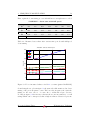
Figure 19 shows the pin configuration of the MCP6S21 programmable gain
amplifier. The positive supply voltage is connected to VDD and the negative
to VSS . VREF defines the reference voltage of the internal non inverting amplifier. This pin is connected to the generated virtual analog ground. CH0
is supposed to carry the input signal of the amplifier and VOUT the amplified
output signal. For more details how to connect the pins of each chip for this
application, see chapter 2.1.4.
The remaining pins SCK, SI and CS are necessary for programming the gain
factor of the amplifier. The MCP6S21 can only operate in slave mode. So
Motorized Guitar Tuner
Weißensteiner, Viehauser
2
FREQUENCY DETECTION
38
the SCK pins of the µ-Controller and the chip were connected, and the SI7
pin has to be connected to the MOSI port of the µ-Controller. To initiate
communication to the chip, the CS8 pin has to be set to digital ground and
is directly connected to an output port of the µ-Controller. Each chip gets
its own output port for the CS pin. Hence the two chips can be programmed
independently.
After setting the CS pin to LO, the MCP6S21 expects a 16-bit instruction
word, consisting of two 8 bit values. The first 8 bit value define the content
of the instruction register.
Figure 20: Screenshot of the MCP6S21 datasheet[2]: Instruction register
Figure 20 shows a screenshot of the datasheet of the MCP6S21 which describes the possible instructions recognized by the chip.
In our application only the “write to the gain register” command configuration is used. Because the MCP6S21 has only one input channel, setting
the channel is not necessary. Also the shutdown functionality is not used.
So according to figure 20, the instruction register has to be set to 0x40 for
reconfiguring the gain.
The second 8 bit value of the 16 bit instruction word defines the new value
of the gain register. Figure 21 shows all possible gain configurations and
7
8
Slave In
(inverted) chip select
Motorized Guitar Tuner
Weißensteiner, Viehauser
2
FREQUENCY DETECTION
39
Figure 21: Screenshot of the MCP6S21 datasheet[2]: Gain register
how they are decoded.
To send the two bytes which are necessary to program one amplifier, the
build in SPI module of the µ-Controller can be used. Before using, it has
to be enabled in the course of an initialize sequence. Listing 1 shows the
initializing of the SPI module. This code sequence sets the data direction
registers (DDR) of the pins which are used for the communication to output mode, sets the CS pins to HI and configures the SPI module of the
µ-Controller by setting 3 flags of the SPI control register (SPCR):
• SPE ... serial peripheral enable: to enable the SPI module
• MSTR ... Master/Slave select: defines the role of the µ-Controller as
master
• SPR0 ... SPI clock rate select: together with the SPR1 flag set to zero,
a clockrate of 1M Hz (fOSC /16) is defined for the SPI bus
1
3
5
// set mosi and sck , cs0 , cs1 as output
DDR_SPI = (1 < < DD_MOSI ) | (1 < < DD_SCK ) | (1 < < SPI_CS0 ) | (1 < <
SPI_CS1 ) ;
// set chips inactive
SPI_PORT |= (1 < < SPI_CS0 ) | (1 < < SPI_CS1 ) ;
// enable SPI , master , set clock rate fck /16
SPCR = (1 < < SPE ) | (1 < < MSTR ) | (1 < < SPR0 ) ;
Listing 1: Initializing the SPI module of the µ-Controller
Motorized Guitar Tuner
Weißensteiner, Viehauser
2
FREQUENCY DETECTION
40
To send the first byte of the 16 bit instruction word after pulling the CS pin
to LO, the byte to send has to be written in the SPDR9 of the µ-Controller.
When updating this register, the data transfer is performed automatically.
After the transfer is finished, the SPIF10 flag is set.
Listing 2 shows the program code of the function which performs the programming of both amplifiers. As argument it expects the gain code of both
amplifiers combined in one byte. This gain code consists of two 4 bit codes
according to figure 21. The combination of the codes for both amplifiers in
one 8 bit value is possible, because only 3 bits are used to decode the desired gain. An internal array of 8 bits per entry was introduced, which maps
exactly the gain table (table 1). An index variable called cur gain number
stores the actual gain level. An increase of the gain can easily performed by
executing spi set gain(gain table[++cur gain number]).
# define SPI_GAIN_INSTRUCTION 0 x40
2
4
6
8
10
void spi_set_gain ( uint8_t gain )
{
// send instruction to SPI0
SPI_PORT &= ~(1 < < SPI_CS0 ) ;
SPDR = SPI_GAIN_INSTRUCTION ;
while (!( SPSR & (1 < < SPIF ) ) ) ;
SPDR = ( gain & 0 x0F ) ;
while (!( SPSR & (1 < < SPIF ) ) ) ;
SPI_PORT |= (1 < < SPI_CS0 ) ;
12
// send instruction to SPI1
SPI_PORT &= ~(1 < < SPI_CS1 ) ;
SPDR = SPI_GAIN_INSTRUCTION ;
while (!( SPSR & (1 < < SPIF ) ) ) ;
SPDR = ( gain >> 4) ;
while (!( SPSR & (1 < < SPIF ) ) ) ;
SPI_PORT |= (1 < < SPI_CS1 ) ;
14
16
18
20
}
Listing 2: programming the gain stages
The gain is controlled by the actual maximal sampled value of the signal.
By introducing two thresholds, the gain level is increased when the maximal
sampled value of the last value series underruns the lower threshold. A
decrease of the gain level is performed when the maximal sampled value
overruns the upper threshold, respectively.
9
10
serial peripheral data register
serial peripheral interrupt flag
Motorized Guitar Tuner
Weißensteiner, Viehauser
2
FREQUENCY DETECTION
2.3.2
41
Recording the signal
2.3.2.1 Ensuring a frequent analog-digital conversion[1] To achieve
a constant sample rate of 8kHz, an internal timer/counter module is used
to trigger the conversion procedure of the analog digital converter. For this
task, the timer 0 is used and can be configured by three registers:
• TCCR0 ... Timer/Counter Control Register 0: defines the operation
mode of the timer/counter 0
• OCR0 ... Output Compare Register 0: stores the value the counter
gets compared with in compare mode
• TIMSK ... Timer/Counter Interrupt Mask Register: defines which interrupts are executed on different events
For this application the clear timer on compare match (CTC) mode is used.
In this mode the counter value of the timer is compared with the OCR0
register and is reset to zero after the contents of the registers match. The
time one increment of the counter value needs is defined by a own prescaler,
which generates a clock (ftimer0 ) depending on the operation clock of the
µ-Controller. To achieve that a compare match occurs exactly 8000 times a
second, a prescaler of fOSC /8 and a compare value of 250 was chosen. With
a system clock of 16M Hz this configuration results a interrupt frequency
(fint ) of
ftimer0 =
fint =
fOSC
16M Hz
=
= 2M Hz
scaler
8
ftimer0
2M Hz
=
= 8kHz
OCR0
250
(11)
(12)
To trigger an interrupt on compare match, the OCIE011 flag of the TIMSK
register must be set to 1.
After the timer is configured to trigger an interrupt 8000 times per second,
the ADC has to be forced to trigger a conversion when this interrupt occurs.
This can be done by setting the ADTS2 to ADTS012 bits in the SFIOR13 register correctly. To start a conversion on a compare match of timer/counter
0, the ADTS2 bit must be set to zero and the ADTS1:0 bits must be set to 1.
Also the ADC has some more options which have to be set. The ATmega32
provides an analog digital converter of 8 channels and two different input
11
Timer/Counter 0 Output Compare Match Interrupt Enable
ADC Auto Trigger Source
13
Special FunctionIO Register
12
Motorized Guitar Tuner
Weißensteiner, Viehauser
2
FREQUENCY DETECTION
42
modes. The two modes are called the single ended input mode and the
differential input mode. In single ended input mode, the absolute analog
voltage is converted to a discrete value, whereas the differential input mode
converts the differential voltage between two channels into its digital representation. In this application the single ended input mode for channel 0
(port ADC0) is used.
Also different reference sources for the ADC conversion circuit can be selected. For this purpose, as reference voltage which represents the highest
possible value in single ended mode, the external AVCC pin is used. This pin
is connected to the positive supply voltage. (When choosing this option, it
is recommended to connect an external capacitor to the AREF pin.)
Since the internal ADC supports a native resolution of 10 bit, the conversion
result needs two 8 bit registers to save its value. These two registers can be
configured as left or right adjusted. A left adjusted setup leads to storing
the most significant bit of the conversion result to the most significant bit
of the higher ordered result register. Because is was decided to use 8 bit
resolution anyway, this option was chosen. So the conversion result equals
the content of the higher ordered conversion result register and value of the
lower ordered conversion result register can be rejected.
To configure the ADC according to these decisions, some bits in the ADMUX14
register must be set. For selecting the AVCC pin as reference voltage source,
the bits REFS1:015 must be set to 0 and 1.
To set the conversion result left adjusted, the bit ADLAR16 must be set to 1.
To define the ADC0 pin as single ended input channel, the MUX4..0 bits must
be all set to 0.
As last step, the ADC control logic has to be told a few settings using the
ADCSRA17 register. For the internal successive approximation converter, also
a clock has to be provided by a configurable prescaler. This can be done by
setting the ADPS2:018 bits.
Also the ADC conversion complete interrupt must be enabled, in whose interrupt service routine (ISR) the result register is read. This functionality
is provided by the ADIE19 flag. Because the ADC should start a conversion
automatically when the timer compare event occurs, the control logic must
enable auto triggering by setting the ADATE20 flag.
Setting the ADEN21 bit is needed to activate the ADC module and make it
ready for conversions.
14
ADC Multiplexer Selection Register
Reference Selection Bits
16
ADC Left Adjust Result
17
ADC Control and Status Register A
18
ADC Prescaler Select Bits
19
ADC Interrupt Enable
20
ADC Auto Trigger Enable
21
ADC enable
15
Motorized Guitar Tuner
Weißensteiner, Viehauser
2
FREQUENCY DETECTION
43
Listing 3 contains the code which is necessary to configure the timer and
the ADC functionalities as described above.
2
4
6
8
void ADC_Timer0_init ( void )
{
// Configure Timer 0
// Prescaler 8 , CTC mode , no output on pins
// TCCR0 :
// FOC0 WGM00 COM01 COM00 WGM01 CS02 CS01 CS00
// 0
0
0
0
1
0
1
0
TCCR0 = 0 x0A ; // 0 b00001010 ;
// compare - register : 250 -> 8 kHz @ 16 MHz clk
OCR0 = 0 xFA ;
10
12
// output compare interrupt enable for timer 0
TIMSK |= (1 < < OCIE0 ) ;
14
// trigger source : timer0 compare match
// SFIOR :
// ADTS2 ADTS1 ADTS0
x
ACME PUD PSR2 PSR10
//
0
1
1
0
0
0
0
0
SFIOR = 0 x60 ;
16
18
20
// AVCC ref with external capacitor , left adjusted
result
// MUX4 ..0: 00000 = single ended ADC0
// ADMUX :
// REFS1 REFS0 ADLAR MUX4 MUX3 MUX2 MUX1 MUX0
//
0
1
1
0
0
0
0
0
ADMUX = 0 x60 ;
22
24
26
28
// auto - triggered mode , interrupt enable , prescaler :
f_osc /128
// ADCSRA :
// ADEN ADSC ADATE ADIF ADIE ADPS2 ADPS1 ADPS0
// 1
0
1
X
1
1
1
1
ADCSRA = 0 xAF ;
30
32
34
}
Listing 3: initialization of the ADC and Timer 0 functionality
2.3.2.2 Starting and stopping a conversion cycle To store the sampled signal temporarily for further processing steps on the µ-Controller, a
global buffer array of 1000 8-bit values is used.
To start a sampling sequence, the ADSC22 flag of the ADCSRA register must
be set to 1. This triggers a frequently conversion cycle with a sampling rate
22
ADC Start Conversion
Motorized Guitar Tuner
Weißensteiner, Viehauser
2
FREQUENCY DETECTION
44
of 8kHz on channel 0, when the initializing was executed correctly. Listing
4 shows the start routine for sampling the signal.
2
4
6
void ADC_start ( void )
{
// initialize the ADC and Timer0
ADC_Timer0_init () ;
// start conversion sequence
ADCSRA |= (1 < < ADSC ) ;
}
Listing 4: ADC start routine
When the ADC module finished a single conversion, the ADC conversion
complete ISR is executed (see listing 5).
This routine saves the new value in its supposed slot in the array. To determine this slot, a global value counter variable was introduced. This counter
variable is also used to determine when the whole array is filled. When the
counter value exceeds the length of the buffer array, the recording stops.
During the recording process of the values stored in the buffer, also the
maximum value is logged. The information of the highest value is used to
adjust the gain of the programmable amplifiers for the next recording cycle.
1
3
5
7
9
11
13
15
ISR ( ADC_vect )
{
// subtract the direct component
int8_t val8 = ( ADCH -128) ;
// log the maximum value
if ( val8 > max_value )
max_value = val8 ;
// store the sample into the sample buffer
values_buffer [ values_cnt ++] = val8 ;
// abortion condition
if ( values_cnt == VALUES_NR )
{
STATUS &= ~(1 < < STAT_RECORDING ) ;
ADC_stop () ; // stop sampling
}
}
Listing 5: Interrupt service routine for finished ADC conversions
2
4
6
void ADC_stop ( void )
{
// stop timer0 interrupts
TIMSK &= ~(1 < < OCIE0 ) ;
// disable ADC
ADCSRA &= ~(1 < < ADEN ) & ~(1 < < ADSC ) ;
}
Listing 6: ADC stop routine
Motorized Guitar Tuner
Weißensteiner, Viehauser
2
FREQUENCY DETECTION
45
Listing 6 shows the stop routine of the recording process. This function
stops the ADC sampling cycle by disabling the triggering timer interrupt
and the ADC itself.
2.3.3
Filtering the signal
To calculate the filtered signal according to figure 11 on the 8 bit architecture
of the µ-Controller, the filter coefficients have to be transformed into the
12 bit fix-point representation. This was done after the filter design in
R
MATLAB
by multiplying the coefficients by 212 followed by a rounding
operation.
Table 6 shows the transform of the filter coefficients of the specialized filter
for the standard D string from floating point to 12 bit fix point representation
for both biquad sections.
Coefficient
a1
a2
b0
b1
b2
a01
a02
b00
b01
b02
Floating point
representation
-1.9813639...
0.9952795...
1.0000
0.0000
-1.0000
1.9826170...
0.9954637...
1.0000
0.0000
-1.0000
12 bit fix-point
representation
-8116
4077
4096
0
-4096
-8121
4077
4096
0
-4096
Table 6: Representation of filter coefficients (specialized standard D)
Due to the high number of filters (and their coefficients), the coefficients
were stored in the flash memory of the µ-Controller using the pgmspace.h
library for AVR. This library allows to save constant variables into the flash
memory by adding the PROGMEM= keyword after the declaration of the name
of the variable. In the developed program, the filter coefficients of all filters
were stored into an array of structs called filters.
To read the stored variables, the pgm read word(&void) function returns
a reference to the desired object. For instance, to get the a1 coefficient
of the current filter indexed by the variable filter nr, int16 coeff =
(int16 t)pgm read word(&filters[filter nr].stg1 a1); has to be executed. stg1 a1 is the struct element in filters, representing the a1 coeffiMotorized Guitar Tuner
Weißensteiner, Viehauser
2
FREQUENCY DETECTION
46
cient of the first biquad stage.
So the filtered value can be calculated by following the graphical instruction
of figure 11. As described in chapter 2.2.6.1, after multiplying two values in
12 bit fix-point representation, the result has to be shifted to the right by
12 binary places. In two’s complement, the sign of signed values is stored
in the most significant bit (MSB). Hence, shifting negative numbers (MSB
is 1) without care leads to wrong results. The solution for this problem,
which takes the least processing time for the µ-Controller, is also the most
intuitive: an if statement.
Listing 7 shows a part of the calculation of the filtered signal. The result of
the multiplication (result) should be subtracted from the variable called
temp. To perform the right shift of the multiplication result, an if statement
checks if the result is negative. If so, the result is transformed to its positive
value, shifted and added to the temp value. Otherwise it is shifted and
subtracted directly.
1
# define FIX_BITS 12
3
result = z1 [0]* ( int16_t ) pgm_read_word (& filters [ filter_nr ].
stg1_a1 ) ;
if ( temp < 0)
{
result = - result ;
result = result >> FIX_BITS ;
temp1 = temp1 + result ;
}
else
{
temp1 = temp1 - ( result >> FIX_BITS ) ;
}
5
7
9
11
13
Listing 7: Multiplication in 12 bit fix-point representation
After finishing the calculation of one filtered value, it is checked for zero
crossing by comparing the sign of the past value with the sign of the new
calculated value. An array stores the previous 4 numbers of samples between
the last zero crossings and a counter variable counts the samples after the
last zero crossing. If a zero crossing occurs, the most previous value of the
array is overwritten by the counter value and the counter gets cleared. After
determining the filtered values of the whole signal, the number of samples
within 4 periods is calculated by summing up the values of the array. The
current frequency information, represented in number of samples within 4
periods, is updated each new recording cycle and can be accessed by the
controlling functions by a global variable.
Motorized Guitar Tuner
Weißensteiner, Viehauser
3
FREQUENCY MANIPULATION
3
47
Frequency manipulation
The frequency manipulation basically consists out of a PID-Controller and a
servo motor what is accessed by Pulse-Width-Modulation. For dimensioning
R
R
the PID-Controller the software MATLAB
/SIMULINK
was used. Two
Guitar models ”Framus” and ”Jackson” have been considered for modeling,
which have both a different kind of torque increase when tuned up.
The following sections will go into detail, describing the specific issues and
resulting solutions.
3.1
Hardware
To provide an automated tuning procedure, a motor is attached on the
tuning pegs (for further details see figure 45). To make this possible certain
requirements have to be fulfilled:
• sufficient motoring torque, about 20 - 35 Ncm
• angular velocity as controlled parameter
• controlling by Pulse-Width-Modulation
• affordability
• advantageous design for application
Two types of motors have been considered based on the requirements above,
a step motor and a servo motor. The disadvantages of a step motor are uncomfortable design and a need of an extra control unit what would have to
be developed to actuate the motor by PWM.
The servo motor on the contrary has a control unit included and is more
affordable than the step motor. Also the design saves more space for developing a hand-held device. The only disadvantage that occurs is the parameter
controlled by PWM, which is the angle itself. To achieve an angular-speed
control the motor has to have the ability to rotate continuously or if its not
able to do so, at least a simple modification should be possible.
Motorized Guitar Tuner
Weißensteiner, Viehauser
3
FREQUENCY MANIPULATION
48
Researches have shown that the servo motor ”Futaba S3003” is very suitable
for the discussed requirements and so the decision was made for this one.
Figure 22: Servo Motor ”Futaba S3003”
Futaba S3003 Specification
Torque
32 Ncm
◦
Speed for 45
0,17 sec
Size
40,1 x 19,8 x 36 mm
Weight
37,2 g
Operation Voltage
4,8 - 6 V
Neutral Impulse
1,52 ms
The servo motor has an included electronic control unit that normally rotates
the drive shaft in its appropriate position according to the PWM signal. The
potentiometer of the main shaft inside the servo is measuring the position
at any given time and so the controller is able to drive the motor properly.
So if the position of the drive shaft is not correct, the motor is moving it
into place by reducing its angular-speed depending on the proximity of the
actual angle to the target angle.
This non-linear characteristic will be exploited to control the angular velocity by the PWM signal.
To achieve this kind of parameter control the servo motor shown in figure
22 has to be modified from position-controlled to rotation-speed-controlled.
The following instructions show how the ”hacking” of the servo motor was
performed.
Motorized Guitar Tuner
Weißensteiner, Viehauser
3
FREQUENCY MANIPULATION
3.1.1
49
Continuous Rotation Modification [3]
1. First of all any wheels or arms that may be attached to the main shaft
were pulled off.
Then the 4 screws on the back of the servo were removed, see figure
23. (Note that it’s not necessary to remove the back of the servo.)
Figure 23: Removing screws
Figure 24: Opening the gear
case
2. Now the gear case (top of the servo) was lifted carefully where it has
to be made sure that the two gear wheels shown in figure 24 may stay
attached to the casing. If they do, they were removed and inserted
into position as shown.
3. The intermediate gear wheel and the main shaft were taken off by just
lifting them, see figure 25.
Figure 25: Lifting Gear Wheels
Motorized Guitar Tuner
Weißensteiner, Viehauser
3
FREQUENCY MANIPULATION
50
4. With fingers or some small pliers the potentiometer shaft was placed
into center position.
Figure 26: Potentiometer shaft
5. Using a thin blade of a razor saw or a cutting disk on a rotary tool, a
small slot was cut in the potentiometer shaft of the servo as shown in
figure 27. This will allow calibrating the servo motor later.
Figure 27: Potentiometer shaft
Motorized Guitar Tuner
Weißensteiner, Viehauser
3
FREQUENCY MANIPULATION
51
6. A small stop had to be removed from the main shaft wheel by using a
small wire cutter.
Figure 28: Main shaft wheel
Figure 29: Main shaft wheel
modified
7. Inside the main shaft wheel were two slots which are used to access the
potentiometer. These slots were removed using a drill bit by reaming
them out carefully.
Figure 30: Main shaft wheel
Motorized Guitar Tuner
Figure 31: Main shaft wheel
modified
Weißensteiner, Viehauser
3
FREQUENCY MANIPULATION
52
8. Drilling through the top of the main gear wheel as shown in figure 32
made it possible to adjust the potentiometer by a micro screw driver.
Figure 32: Potentiometer shaft
9. Then the main shaft wheel was inserted again into the top of the servo
chassis as shown in figure 33.
Further it was assembled with the potentiometer where it should rotate freely without catching.
Figure 33: Testing the main shaft wheel
Motorized Guitar Tuner
Weißensteiner, Viehauser
3
FREQUENCY MANIPULATION
53
10. At last the two gear wheels were reassembled and some oil was added.
The casing was reattach again with the 4 rear screws.
Figure 34: Reassembling the servo motor
11. To calibrate the servo a control signal with 1500µs PWM (neutral position) was generated and the potentiometer was adjusted with a micro
screw driver through the main shaft hole until the drive shaft stopped
rotating.
Figure 35: Calibrating the servo motor in neutral position
After these steps the servo motor has the ability to control the angular
velocity and to rotate continuously as needed to tune a guitar.
Motorized Guitar Tuner
Weißensteiner, Viehauser
3
FREQUENCY MANIPULATION
3.1.2
54
Servo control by ATmega32
To control the servo motor Pulse-Width-Modulation is used. The µC ATmega32 provides two 8-bit Timer/Counter and one 16-bit Timer/Counter,
each with separate prescalers and three different kinds of PWM operation
modes.
Before the timer resolution and prescaler value is considered, the appropriate PWM operation mode has to be chosen. For this the micro-controller
provides ”Fast PWM Mode”, ”Phase Correct PWM Mode” and ”Phase and
Frequency Correct Mode”.
3.1.2.1
Fast PWM Mode
This mode is able to generate a high frequency PWM waveform by its singleslope operation. The counter counts from bottom to top, then restarts from
bottom. Due to the single-slope operation, the operating frequency of the
fast PWM mode can be twice as high as the other two PWM modes which
use dual-slope operation.
The PWM resolution for fast PWM can be fixed to 8-bit, 9-bit or 10-bit.
For the two last ones the 16-bit timer 1 has to be used. The counter is
incremented until its value matches either one of the fixed values (example:
0x00FF for 8-bit), then it is cleared and restarts again.
Figure 36 shows the timing diagram which illustrates the single-slope operation. The small horizontal line marks on the TCNT1 slopes represent
compare matches between OCR1x and TCNT1. In non-inverting mode the
output compare OCnx pin is then set to LOW and this causes the ”end” of
the pulse. The counter continues counting up until the sequence is restarting
again. [1]
Figure 36: Fast PWM timing diagram [1]
Motorized Guitar Tuner
Weißensteiner, Viehauser
3
FREQUENCY MANIPULATION
3.1.2.2
55
Phase Correct PWM Mode
Based on a dual-slope operation, this mode provides a high resolution phase
correct PWM waveform generation option. The counter counts repeatedly
from bottom to top and then from top to bottom. In non-inverting compare
output mode, the output compare (OC1x) is cleared on the compare match
between TCNT1 and OCR1x while upcounting, and set on the compare
match while downcounting.
The dual-slope operation has lower maximum operation frequency than single slope operation. See the timing diagram in figure 37 for illustration.
[1]
Figure 37: Phase Correct PWM timing diagram [1]
3.1.2.3
Phase and Frequency Correct Mode
This mode provides a high resolution phase and frequency correct PWM
waveform generation option. Like the phase correct PWM mode mentioned
before, a dual-slope operation is used. The counter counts repeatedly from
bottom to top and then from top to bottom. The output is generated like
in the phase correct PWM mode.
The main difference between the phase correct and the phase and frequency
correct PWM mode is the time the OCR1x Register is updated by the
OCR1x Buffer Register, see figure 37 and figure 38. [1]
Motorized Guitar Tuner
Weißensteiner, Viehauser
3
FREQUENCY MANIPULATION
56
Figure 38: Phase Correct PWM timing diagram [1]
For further details concerning the different PWM modes it is referred to the
datasheet [1].
To achieve a simple and prompt PWM waveform control that suits best
for the servo motor and offers a plain software implementation, the fast
PWM mode is applied. Therefore only the two OCR1x registers have to be
set to define the proper pulse-width with constant period time (see figure 36).
In addition to the selected operation mode the appropriate parameters have
to be resolved.
To check which combination out of bit-resolution and prescaler value at
the given clock rate of 16MHz allows a smooth motor control, several pulse
periods have been considered, shown in table 7.
FRAMUS - up tune with full speed
Pulse-Periods
Prescaler
1
8
64
256
1024
8 bit
0.016 ms
0.128 ms
1.024 ms
4.096 ms
16.384 ms
Fast-PWM-Resolution
9 bit
10 bit
16 bit
0.032 ms
0.064 ms
4.096 ms
0.256 ms
0.512 ms
32.768 ms
2.048 ms
4.096 ms
262.144 ms
8.192 ms
16.384 ms 1048.576 ms
32.768 ms 65.536 ms 4194.304 ms
Table 7: Pulse time periods at different timer configurations
The 16MHz external clock rate (quarz) is divided by the prescaler and defines the frequency of the timer. For a 16-bit resolution timer 1 has to
be used. The neutral-pulse of 1500µs duration has to occur at least every
16.384ms, marked green. If this time period is reduced below this value,
Motorized Guitar Tuner
Weißensteiner, Viehauser
3
FREQUENCY MANIPULATION
57
the servo motor starts to vibrate due to the fact that one period is actually
reinterpreted as one pulse.
The second aspect is the resolution of the count value related to the timer.
This value has to be incremented and decremented to set the certain pulsewidth and if the minimal possible step is too inaccurate, also the servo access
would be so. It turned out that a period length of 16.384ms, independent
of the resolution, only allows a minimal pulse-width grading of 16µs, which
has shown to be not very precise for varying the angular velocity.
Hence, the 16-bit timer with the prescaler value of eight was chosen, marked
yellow in table 7. This period length seems nearly too long, but the grading
of the pulse is fine enough with 0.5µs.
With this configuration it is now possible to actuate the servo motor in both
rotation directions. The neutral position is defined with 1500µs PWM, at
where the motor is not rotating and trying to hold its position with a certain
torque. This neutral control pulse is later on software-defined ”zero”. This
zero-point allows a setup with either negative or positive values, accordingly
to the rotation direction. Experiments have shown that the Futaba S3003
has its full strength at a value about ±300, which means a pulse-length of
±300 ∗ 0.5µs = ±150µs.
In chapter 3.3 the setup with value 300 will also be called as full speed tuning.
3.1.3
Servo voltage supply
The current required by the servo motor while rotating causes disruptions
on the voltage supply. Even worse is the start-up process of the servo, which
temporarily can take about 600mA. This short-term consumption cannot
be supported by the voltage regulator and may lead to voltage drop out
causing micro-controller malfunction.
To avoid this, a capacitor with 470µF (6V) was applied to the voltage supply
which provides more stability.
Motorized Guitar Tuner
Weißensteiner, Viehauser
3
FREQUENCY MANIPULATION
3.2
58
Control theory
Basically, control theory deals with the analysis and design of closed loop
control systems. So the main structure in control systems is based on negative feedback. The goal in control of physical systems is to track the output
signal (e.g. frequency, room temperature, speed of a motor, level of a tank,
etc.) according to a reference signal and to reject the effect of the disturbances.
Furthermore it has to be distinguished between a system that has to be
controlled and the whole control system itself. The requirements of a control system are dependent of its type, distinguishing between discrete digital
implementation and analog continuous operation. First of all it has to be
stable, so that no oscillating occurs. Then, it has to meet the quality specifications for steady-state accuracy, dynamic properties such as overshoot,
setting time, latency, etc. Also the control signal which actuates a system
input has to be inside its technical limits (anti-windup). In addition to that
a control system has not to be very sensitive to measurement noise and to
plant/model mismatch.
The following block diagram (figure 39) illustrates the schema of the feedback loop control system or closed-loop control system.
Figure 39: Closed-loop control system [6]
The so called system is also known as plant or process. A real physical
system is represented by a mathematical model which is used for analysis
and designing a appropriate control system. The math behind a plant is also
represented as a transfer-function which delivers a certain output regarding
of a temporary input.
The output value of a plant is then being measured by a sensor and compared to a reference value by subtracting. The resulting difference called
error is then amplified or modified by the controller to create the control
signal. This signal affects the input of the process in order to reach the
desired behaviour.
In this structure the output signal is fed back to the input of the plant, thus
the controlling is realized by negative feedback.
Before going further into control theory, it has to be mentioned that it conMotorized Guitar Tuner
Weißensteiner, Viehauser
3
FREQUENCY MANIPULATION
59
sists of way too many topics of detail to discuss all of them, so only the
basics are treated.
In feedback systems the execution of the control command is always delayed to a certain degree, because of inherent delays and dead time in the
individual (electronic) components. This disturbing effect is a general part of
digital discrete control systems. Therefore unstable behavior may be evoked
when steady or increasing oscillations do appear in the process output.
This has to be avoided.[7] Hence disturbances will always occur in real-life.
The sensor shown in figure 39 is, as already mentioned, measuring the actual output value of the plant. Control system components sometimes act
as controller and sensor simultaneously (like our µ-Controller).
Basically, the control operation can be described with several mathematical terms individually or in combination. Therefore the most common type
of controller is used, the so called PID controller which is named after its
three correcting therms, the proportional term, the integral term and the
derivative term. The PID controller can be used to control any measurable
variable, as long as this variable can be affected by manipulating some other
process variables [8].
Before the PID Controller is considered in 3.2.4, the respective terms will
be discussed individually.
3.2.1
Proportional term
The proportional term is providing an overall control action proportional to
the error. This is done by multiplying the factor Kp , called the proportional
gain, with the error signal.
The proportional term is given by:
P (t) = Kp ∗ e(t)
(13)
Increasing the proportional gain Kp causes in general a small increase of the
setting time and a light decrease of the steady-state error, but may degrade
the stability of the control system. In this case, the term value may increase
too quickly and will ”overshoot” the desired value. In worst case the control loop will begin to oscillate around the target value which is also called
”hunting”. If the gain is determined too low, the controller is less sensitive
Motorized Guitar Tuner
Weißensteiner, Viehauser
3
FREQUENCY MANIPULATION
60
and may compensate disturbances too slow.
Figure 40 shows a response to the proportional gain without overshoot.
Figure 40: Response to P (t) at set-point = 10 over time [9]
In fact, the proportional term alone will rarely reach the desired target value
which results in a steady state error, because of drift by analog components
or quantization error in digital controllers.[9]
As a matter of this, discrete control systems will never be able to eliminate
a steady-state error completely, so further accuracy requirements have to be
fulfilled.
3.2.2
Integral term
The integral term corresponds to the error magnitude and the error duration. The error is summed up over time and gives an accumulated value
which is multiplied with the integral gain Ki . Typically this is used to get
rid of offset error. As long as the target value is missed, the integral term
will change accordingly (permanent).
Motorized Guitar Tuner
Weißensteiner, Viehauser
3
FREQUENCY MANIPULATION
61
The integral term is given by:
Zt
I(t) = Ki ∗
e(τ ) dτ
(14)
0
This term acts like a kind of weight traced by the controller which is also
called ”memory”, because difference values of the past are considered. If the
integral gain Ki is set too high, the control system easily tends to overshoot
and begins to oscillate. On the other side, with a too low gain the individual
term looses its control-effect and causes a very slow control behaviour. However, the integral term is widely used together with at least the proportional
term.
In the diagram of figure 41 you can see the proportional response and the
integral response. Also a combinational response of these is shown.
Figure 41: Responses to I(t) and P (t) at set-point = 10 over time,
p...proportional term, i...integral term, pi...combination of the two terms
[9]
The main advantages of the integral term are an improvement of the setting
time and an elimination of the steady-state error. So an aberration to the
target value caused by the proportional term may be wiped out.
Regarding a digital discrete control system also the integral term can’t prevent a persistent real error which is discussed later in chapter 3.2.4.
Motorized Guitar Tuner
Weißensteiner, Viehauser
3
FREQUENCY MANIPULATION
3.2.3
62
Derivative term
This term is typically used in combination with a proportional term and/or
an integral term, because here not the magnitude of the error is regarded
but its changing speed. This improves the response to a sudden change in
the system state or reference value. So the error value is derived by time as
the following equation shows.
D(t) = Kd ∗
de(t)
dt
(15)
So if the error has a constant change in its value the derivative term delivers an constant output dependent on the factor Kd . Because of this the
derivative term will never be able to control by its own.
In figure 42 the responses between proportional term and derivative gain are
shown.
Figure 42: Responses of D(t) and P (t) at set-point = 10, p...proportional
term, d...derivative term, pd...combination of the two terms [9]
Generally it is very difficult do determine the derivative gain Kd properly
because, on the one hand this term reduces the overshoot caused by an
integral component, but on the other hand noise is amplified as well as the
signal change and so if the gain is set too high the whole control system
could become unstable quickly. So the derivative term can also be seen as a
kind of high-pass filter.
Motorized Guitar Tuner
Weißensteiner, Viehauser
3
FREQUENCY MANIPULATION
63
Basically the response of a PD controller leads to a faster rising time than
a single P controller but it is also impossible to prevent steady-state errors
without an additional integral term. [8]
3.2.4
PID controller
In general the PID controller is designed with three terms (these are discussed in chapters before), which manipulate the controller input known as
error in three ways: to handle the present, through the proportional term;
recover from the past, using integral term; and to anticipate the future,
through the derivative term [8].
Figure 43 shows a schematic block diagram of a control system with PID
controller.
Figure 43: PID controlled loop [10]
A PID controller uses all three terms by adding the outputs together, which
then actuates as control signal for the plant. The ideal parallel form for
calculating the control output C(t) is done in equation 17.
C(t) = P (t) + I(t) + D(t)
Zt
C(t) = Kp ∗ e(t) + Ki ∗
e(τ ) dτ + Kd ∗
(16)
de(t)
dt
(17)
0
For an illustration of the resulting behaviour the following diagram is shown
with different kinds of controllers.
All in all, using all terms together usually gives the best performance. In
figure 44 the PI controller improves the result by removing the stationary
error leafed by the proportional term and the PID controller again improves
Motorized Guitar Tuner
Weißensteiner, Viehauser
3
FREQUENCY MANIPULATION
64
Figure 44: Varying controller types compared [9]
the result of the PI by faster response and no overshoot.
To determine the proper gain values for the certain terms several tuning
methods exist. Often a detailed mathematical description of the system is
unavailable due to missing measurable values and/or formulas representing
the process. For this experimental tuning of the PID parameters has to
be performed. Finding the terms is often a challenging task and so good
knowledge about the systems properties and the way the different terms
work is essential.
The optimum behavior on a process change or set-point change depends on
the application at hand. For some control systems an overshoot has to be
prevented, others demand less energy consumption in reaching the target
value. Typically, stability is the strongest requirement by designing a controller. [8]
The other methods for dimensioning, of course, do rely on some mathematical approximations. The choice of method will depend largely on whether
the process can be taken off-line for tuning or not. The Ziegler-Nichols
method is a well known online tuning strategy. The first step in this method
is setting the integral term and the derivative term to zero, increasing the
proportional gain until a sustained and stable oscillation (as close as possible) occurs on the output. Then the actual gain called critical gain Kc
and the correspondent oscillation period Pc is recorded and the P, I and D
parameters are adjusted accordingly using table 8. [8]
The time constants Ti and Td are then used to calculate the Ki and Kd
Motorized Guitar Tuner
Weißensteiner, Viehauser
3
FREQUENCY MANIPULATION
65
Controller
Kp
Ti
P
0.5 ∗ Kc
PD
0.65 ∗ Kc
PI
0.45 ∗ Kc
0.85 ∗ Pc
PID
0.65 ∗ Kc
0.5 ∗ Pc
Td
0.12 ∗ Pc
0.12 ∗ Pc
Table 8: Ziegler-Nichols method paramters
factors as follows:
Ki =
Kp
Ti
Kd = Kp ∗ Td
(18)
(19)
Further tuning of the parameters is often necessary to optimize the performance of the PID controller.
Another tuning method that is considering the step response of the plant is
done by opening the control loop. The step response is then recorded and
analysed. For this, the steepest tangent of the rising curve at the beginning is determined and intersected with the maximum and minimum level
of the response. The so triggered time periods are then measured and used
for tuning the PID parameters with the rules of Chien-Hrones-Reswick,
which will not be discussed further. Here, also the Ziegler-Nichols method
can be applied.
Parameters also can be found by simulating the control system with common computer software. Hence, a system model has to be created preferably
as an exact representation of the real world system. This requires in most
cases the knowledge of the mathematical background that describes the real
world model best.
(The decision has fallen to this kind of parameter tuning although we did
not have a mathematical model of our plant. Therefore it is referred to
chapter 3.3.)
Motorized Guitar Tuner
Weißensteiner, Viehauser
3
FREQUENCY MANIPULATION
66
There exist several other dimensioning methods like using the Bode-diagram
(frequency based method) which will not be considered in this context.
3.2.4.1
Discrete PID controller
”A discrete PID controller will read the error, calculate and output the
control input at a given time interval, at the sample period T . This sample time should be less than the shortest time constant in the system.”[8]
Because of this, the calculation of the control signal could not be done like
in equation 17 anymore. Due to the fact that time is not continuous in
this case, constant sample time and system defined latency are important
aspects respectively to the integral term and the derivative term, which are
calculated time dependent.
To process an discrete/digital output, the individual control terms have to
be transformed into a discrete form. The integral can be regarded as a sum
of values over the number of samples.
Zt
e(τ ) dτ ≈ T ∗
n
X
e(k)
(20)
k=0
0
The derivative term can be represented as difference between the actual
error and the error before.
de(t)
e(n) − e(n − 1)
≈
dt
T
(21)
Where n is the discrete step at time t and T is the sample time period. So
the time t = n ∗ T . [8]
This gives a controller output:
C(n) = Kp ∗ e(n) + Ki ∗
n
X
e(k) + Kd ∗ (e(n) − e(n − 1))
(22)
k=0
Where, for Ziegler-Nichols tuning, the gains are:
Kp ∗ T
Ki =
Ti
Kp ∗ Td
Kd =
T
Motorized Guitar Tuner
(23)
(24)
Weißensteiner, Viehauser
3
FREQUENCY MANIPULATION
3.2.4.2
67
Integral windup
By the reason that every controller, especially a digital one, has its output signal limitation, it has to be made sure that a growth of the integral
term does not produce a control output signal that is beyond its limitations.
If so, the controller is calculating internally a value that can’t be used for
actuating, that’s why the PID controller will then overcompensate the process input until the integral sum is back to normal.
This problem can be avoided in several ways, for example limiting the sum
by not allowing it to become larger or lower than a certain value. This
limitation value always depends on the system and the sample time used.
Motorized Guitar Tuner
Weißensteiner, Viehauser
3
FREQUENCY MANIPULATION
3.3
68
R
System modelling with MATLAB
/Simulink
R
R
R
For modelling our control system loop the software MATLAB
/Simulink
was
used which provides tools for designing and developing control systems and
models. Furthermore, the Simulink Control Design GUI provides a graphical environment for control system linearization and design. Additionally,
settings can be restored and saved as well as results can be exported to the
R
MATLAB
workspace. [11]
Before our Simulink control system model will be shown and discussed in
3.3.3, the following section will explain the behavior and characteristics of
the individual real-world components.
3.3.1
Guitar
When someone buys a guitar there is never some kind of datasheet thereby
which describes the the product behavior mathematically. Anyway, to create
a virtual model of our guitar, researches have shown that some basic formulas
about string oscillation and frequency-torque relation are very convenient for
modeling.
A quick overview about the parts of an electric guitar shows figure 45.
Figure 45: Electric guitar parts [12]
Motorized Guitar Tuner
Weißensteiner, Viehauser
3
FREQUENCY MANIPULATION
69
The six strings of a guitar can freely oscillate between the nut and the bridge.
When a chord is played the fingers shorten the oscillating string so that the
tone is heightened. At tuning the guitar the strings are not touched to allow
the appearance of each lowest possible frequency. To record a frequency signal the pickups of an electric guitar seems very comfortable but also acoustic
guitars strings could be measured by microphone.
We just decided to use only electric guitars for tuning because most acoustic
guitars also have a too high string torque that cannot be handled by our
chosen servo motor ”Futaba S3003”.
Generally, to determine certain characteristics two guitar models were available. A vintage model FRAMUS - Billy Lorento 10 which was manufactured
R
in 1969 and a JACKSON
Soloist SL2H (Limited Sam Ash Edition).
(a) Framus BL10
[13]
R
(b) Jackson
Soloist
SL2H [14]
Figure 46: guitar models used for modeling
The vintage model, of course, was more difficult to handle with regarding the
servo motor torque limit but this will be explained in detail in the following
sections.
Motorized Guitar Tuner
Weißensteiner, Viehauser
3
FREQUENCY MANIPULATION
3.3.1.1
70
Guitar string analysis
First it has to be mentioned that there exist various kinds of strings with different thickness, material and manufacturing technique which all influences
the oscillating characteristics. In this case a matter of particular interest
would be the relation between the string frequency change and the string
tension change (which also results in torque change on the machine heads
or tuning pegs).
Basically, if a string is oscillating a musician talks about a tone where a
technician talks about frequency. It is also known that if a string is shortened the frequency would raise. As a matter of fact, if the oscillating string
length is halved, the frequency is doubled. Regarding the tuning process
here, the length of the string would always stay the same (from bridge till
nut), so a relation between the tension-force and the frequency has to be
found.
In oscillation physics the frequency always mentioned in this context would
be the fundamental frequency f0 which is defined as the lowest frequency of
a periodic waveform’s spectrum.
The fundamental frequency of a guitar string is given by
p
p
Ψ/πρ
Ψ[N ]
f0 = n ·
=
· 6, 3Hz
D·L
D[mm] · L[m]
(25)
[15]
Using n = 1 (fundamental frequency) Ψ is the tension-force, ρ the material
density, D the string diameter and L the length of the string. To calculate
the necessary tension-force Ψ, the fundamental frequency and the string
length will be multiplied together, and so if the tension-force is constant the
string length and the frequency are acting reciprocal to each other (which
has already been discussed before).
Ψ = (f0 · L)2 · πρD2
(26)
[15]
So if we want to double the frequency, the tension-force has to be increased
four times.
Regarding equation 25 by contracting constant variables to ξ, the relation
becomes more obvious.
Motorized Guitar Tuner
Weißensteiner, Viehauser
3
FREQUENCY MANIPULATION
√
f0 =
71
Ψ·ξ
(27)
The next step is to find out how the servo motor affects the tension-force or
the according torque. If the servo motor is driving a tuning peg at a certain
angular speed, the tension-force increase is proportional to an integral over
time. So the following equation seems valid due to guitar experiments.
Zt
ω · (η(Ψ) + 1) dτ
Ψ(t, ω) =
(28)
0
This equation is recursive because of η, which represents a tension dependent
resistance that will counteract the angular velocity ω. This resistance grows
with the string tension and the servo motor can’t actuate constantly anymore
although there is a constant control signal. In order to that, the control
signal has to adapt to this inconvenient behavior, which is discussed in
3.3.1.2.
If we now substitute the tension-force in equation 27 we get
v
uZt
u
u
f0 = ξ · t ω · (η(Ψ) + 1) dτ
(29)
0
which is again a recursive equation. We do not actually have to calculate
with this recursive formula because we just use the individual terms of it for
developing a model in Simulink.
All in all, the frequency depends on a constant factor ξ defined by the
string physics, the integral of the actual angular velocity ω and a torque
dependent resistance η. With these basic mathematical considerations we
are now able to form a software supported model approximation.
Motorized Guitar Tuner
Weißensteiner, Viehauser
3
FREQUENCY MANIPULATION
3.3.1.2
72
Guitar string modeling
Simulink provides a huge repertory of graphical elements that can be combined together to form a representation of a ”real world” system. In this
case it’s needed to model a guitar string which then could be used for simulating a control system loop.
In equation 29 the various terms of the string behavior are shown. Before
the complete string model is specified, it has to be mentioned that a continuous integral form in Simulink is always described as a Laplace transformed
term.
Zt
f (u) du
c
s
1
F (s)
s
(30)
0
By this reason we use the integrator block for integrating the certain value
and then extract the root of it with the square-root block. These two blocks
are responsible for the main characteristics of a guitar string. But we will
also need a few more components to fulfill equation 29.
Before going into detail let’s first consider the developed model that repreR
sents an approximation of the D-string of the guitar model Jackson
Soloist
SL2H in figure 47.
As input the angular velocity acting at the tuning pegs was defined. Furthermore, a separation of the signal in two different ”modes” was made because
experiments have shown that one strings behaviour also differs in tuning up
(frequency increase) or tuning down (frequency decrease) in unexpected big
relations. This becomes obvious considering the actual string tension that on
the one hand supports the down tuning procedure at decreasing the torque
and on the other hand counteracts the up tuning process at increasing the
torque. So the higher the absolute string frequency the more torque has to
be applied if tuning up further. And even this effect is varying between all
six guitar strings due to differences in string material and dimensions.
Additionally, there are two slackness blocks” (see figure 47) that characterize the effect of a certain dead-time interval of the angular speed. This is,
because when the servo motor creates a too low mechanical torque for rotating the tuning pegs it would not be able to do so. Experiments revealed
that up-tuning causes a wider dead-time interval. Also this effect is varying
from string to string. For easier approximation a constant torque slickness
over all six strings was assumed.
Motorized Guitar Tuner
Weißensteiner, Viehauser
Motorized Guitar Tuner
1
omega
Torque Slackness UP
u1
if(u1 > 0)
Torque Slacknesss DOWN
If
elseif(u1 < 0)
Gain
1
In2
In1
In2
In1
UP
elseif { }
DOWN
if { }
Out2
Out1
Out2
Out1
Add1
Add
String
Factor
Up
130
String
Factor
Down
120
0.07
increasing
Resistance
0.1
decreasing
Resistance
1
s
Initialization
u2
Tension
Force
xo
|u|
Start
Taus
208
Tension to
Frequency
1
taus
3
FREQUENCY MANIPULATION
73
Figure 47: Guitar string model, string D
Weißensteiner, Viehauser
3
FREQUENCY MANIPULATION
74
After the torque slackness has affected the model input value ω, the ”data
lane” now splits up into two boxes - DOWN and UP. These two boxes are
linked with an if-conditioned box, which actuates with a logical signal each
of them. So if the input ω (defined as u1 in the if-box) is positive, the
DOWN -box is active and the modeled motor is tuning the string down.
Otherwise the motor would tune the string up.
Figure 48 shows the content of the boxes ”DOWN” and ”UP”.
(a) DOWN Block of figure 47
(b) UP Block of figure 47
Figure 48: Content of conditioned blocks
The two blocks are actually calculating the term ω ∗ η, and on the outside
the two outputs Out1 and Out2 are then added together to form the term
ω ∗ (η + 1). Now, an integrator component has to follow from which a square
root has to be taken afterwards, so equation 29 will be designed completely.
As plant output the previously defined number of samples within 4 periods
unit is used (for further explanation read chapter 2.2.1). In the following
sections this frequency dependent unit will also be called ”taus-value”.
The last step was to find out those gain values of the guitar string model
that provide an approximation of the string physics factor ξ (string factor)
and the matching torque dependent resistance η. Concerning the up/down
tuning process, four different gain values have to be determined. To do this,
some empirical measurements on both guitars were made.
At first the FRAMUS guitar model was inspected. Therefore, all six strings
have been up-tuned and down-tuned for various periods of time with full
servo motor torque. Then the resulting taus-values were noted and plotted
to see the different string relevant performances.
Motorized Guitar Tuner
Weißensteiner, Viehauser
3
FREQUENCY MANIPULATION
75
FRAMUS - down tune with full speed
Strings
E
A
D
G
H
e
Before
388
291
218
163
130
97
After 0.5sec
427
307
230
174
135
100
After 1sec
499
351
261
195
149
105
After 1.5sec
600
390
293
234
161
110
Table 9: Measured taus-values after various time periods with full-speed
down tuning
FRAMUS − down tune with full speed
600
before
after 0.5sec
after 1sec
after1.5sec
500
taus−value
400
300
200
100
1
1.5
2
2.5
3
3.5
x−th String
4
4.5
5
5.5
6
Figure 49: Plot of measured values of table 9 over strings (guitar FRAMUS )
As illustrated in figure 49 and figure 50, all six strings have different frequency decrease (or taus increase) by tuning with same motor strength.
Especially the first string, the lower E (1th string), has an immense frequency decrease against the sixth string, the higher e (6th string).
This is due to the fact that in music theory the frequency always raises by
the factor of two every octave step. In our case the measured periods (taus)
will increase reciprocal to it. So, the lower the frequency the higher the
measured taus will be.
Motorized Guitar Tuner
Weißensteiner, Viehauser
3
FREQUENCY MANIPULATION
76
FRAMUS − down tune with full speed
E
A
600
D
G
500
H
taus−value
e
400
300
200
100
0.2
0.4
0.6
0.8
time in seconds
1
1.2
1.4
Figure 50: Plot of measured values of table 9 over time (guitar FRAMUS )
The increasing relations are plotted in figure 51, which show an average
increase of about 1.75 times every half second with full servo strength. Only
the fourth string D shows inconsistency which can be explained by a replaced
new machine head (which was done by the other owner before).
Keeping these facts in mind for later conclusions the up-tuning behavior of
all strings is tested, again with full servo motor strength.
FRAMUS - up tune with full speed
Strings
E
A
D
G
H
e
Before
388
291
218
163
130
97
After 1sec
371
287
204
154
161
96
Before
438
331
258
193
150
107
After 1sec
395
313
228
175
139
103
Table 10: Measured taus-values by tuning up with full speed at different
start values
Motorized Guitar Tuner
Weißensteiner, Viehauser
3
FREQUENCY MANIPULATION
77
FRAMUS − increase relations
2.3
0.5sec − 1sec
2.2
1sec − 1.5sec
shape−preserving interpolation
2.1
shape−preserving interpolation
increase relations
2
1.9
1.8
1.7
1.6
1.5
1.4
1.3
1
1.5
2
2.5
3
3.5
x−th String
4
4.5
5
5.5
6
Figure 51: Plot of increase relations every half second when tuning down
w.r.t. the start values (guitar FRAMUS )
For table 10 two different start values were adjusted and both times one
second was tuned up. This was done because tuning-up experiments have
shown that also the start value has an big impact on tuning behaviour due
to current string tension forces.
High start frequencies means that the taus-values are at the beginning set
like when the guitar is in right tune. Then the start values were set a little
bit below the desired ones to see the detuned behavior.
Like in the plot of the down-tune experiment in figure 49, the up-tuning
procedure acts in a similar relation between the six strings. Only the increasing tension resistance η causes a more difficult up-tuning of the servo
motor, so the value-changes measured here are smaller.
Motorized Guitar Tuner
Weißensteiner, Viehauser
3
FREQUENCY MANIPULATION
78
FRAMUS − up tune with full speed in 1sec
450
high start frequency
high end frequency
low start frequency
low end frequency
400
350
taus−value
300
250
200
150
100
50
1
1.5
2
2.5
3
3.5
x−th String
4
4.5
5
5.5
6
Figure 52: Plot of measured values when tuning 1sec up with full speed
(guitar FRAMUS )
Up to here, the characteristic curves of the vintage guitar model FRAMUS
R
had been gained. The second considered guitar model JACKSON
Soloist
was expected to be more comfortable for the tuning process because of novel
tuning pegs which need less motor torque for rotating compared to the
guitar discussed before. By that reason the time periods the servo motor
was rotating in were graded finer for getting a more accurate end-result.
Furthermore, it has to be said that at testing this guitar the second string
A was not available (unfortunately caused by damage).
Motorized Guitar Tuner
Weißensteiner, Viehauser
3
FREQUENCY MANIPULATION
79
First, again the down tuning process with full motor strength was recorded.
JACKSON - down tune with full speed
Strings
E
A
D
G
H
e
Start
388
291
218
163
130
97
125ms
395
220
164
131
97
250ms
402
221
166
132
97
375ms
414
223
168
133
98
500ms
432
226
174
136
99
1sec
520
241
189
143
101
1.5sec
598
260
213
152
104
Table 11: Measured taus-values after various time periods with full-speed
down tuning
JACKSON − down tune with full speed
600
E
D
G
500
H
e
taus−value
400
300
200
100
0
0
500
1000
1500
time in msec
Figure 53: Plot of measured values of table 11 over time (guitar JACKSON )
Considering the two plots in figure 53 the same effect like mentioned at downtuning of the previous guitar occurs. The lower the frequency the easier the
tuning for the servo motor, of course due to additional torque decrease.
Looking at figure 54 the increase relations show some inconsistency over all
strings which can be interpreted that a high non-linear behavior is present.
Motorized Guitar Tuner
Weißensteiner, Viehauser
3
FREQUENCY MANIPULATION
80
JACKSON − increase relations
2
0.5sec − 1sec
1sec − 1.5sec
1.8
shape−preserving interpolation
shape−preserving interpolation
increase relations
1.6
1.4
1.2
1
0.8
1
1.5
2
2.5
3
3.5
4
x−th String, 1...lowE, 2...D, 3...G, ....(A is missing)
4.5
5
Figure 54: Plot of increase relations every half second when tuning down
w.r.t. the start values (guitar JACKSON )
Continuing with the research about tuning up, the further values had been
captured in table 12.
JACKSON - up tune with full speed
Strings
E
A
D
G
H
e
Start
398
291
228
168
135
100
125ms
396
227
166
135
100
250ms
392
225
165
134
100
375ms
384
223
164
133
100
500ms
378
222
162
131
99
1sec
357
217
156
126
98
Table 12: Measured taus-values after various time periods with full-speed
up tuning
Compared to the up-tuning table 10 of the FRAMUS model, table 12 involves time periods below a second. Like the detailed time resolution of
the down-tuning records, this allows an explanation of the short-period behaviour of the motor/string dependencies.
At tuning up, the counteracting string-tension-dependent resistance η seems
Motorized Guitar Tuner
Weißensteiner, Viehauser
3
FREQUENCY MANIPULATION
81
JACKSON − up tune with full speed
400
E
350
D
G
300
H
taus−value
e
250
200
150
100
50
0
100
200
300
400
500
600
time in msec
700
800
900
1000
Figure 55: Plot of measured values when tuning up with full speed (guitar
JACKSON )
to become a problem. The higher frequency strings H and high e have a
too small changing in their taus-values which leads to inaccuracy regarding
the maximum resolution of the internal ADC. This unfortunately causes less
accuracy in tuning.
To sum up, the investigation of the two guitars has shown a slightly different
R
behavior. Nevertheless, the decision was made for the model Jackson
Soloist
due to easier handling by the chosen servo motor.
With the previously achieved data and characteristic curves it is now possible to complete our string model by designing the four gain factors, 2 x
String factor (ξ) and 2 x increasing/decreasing resistance (η) (see figure 47).
To show how this was done, the designing method for the D-string will be
explained.
Motorized Guitar Tuner
Weißensteiner, Viehauser
3
FREQUENCY MANIPULATION
82
Generally, a system model can be configured regarding the response curves.
It is referred to figure 47 for the following descriptions. At first we want
to achieve the gain factors for the down-tuning part of the model, so
the start value of the integral component has to be set accordingly to the
taus-value of the D-string in table 11 (which actually is 218). The model
input omega is set to its maximal possible magnitude to simulate the virtual
full strength of the motor. Then the output taus is scoped to get the response curve visualized. Figure 56 shows the response output of the already
adjusted model. The red boxes represent the certain time points at where
the resulting virtual taus-values have to be adapted to the determined ones
out of table 11. This was done by varying the gain factors till such time as
the required characteristic curve arises.
Model response by tuning down with full speed
270
Response
260
has to be 241
at one second
taus−value
250
240
230
220
210
200
0
200
400
600
800
1000
time samples, at 800 samples per second
1200
Figure 56: Plot of model response at 800 samples per second
In order to this, the same designing procedure was done with the up-tuning
part of the model.
The delivered signals given by the up/down tracks in the model are then integrated and square-rooted to fulfil the last parts of our frequency equation
29.
Motorized Guitar Tuner
Weißensteiner, Viehauser
3
FREQUENCY MANIPULATION
83
All in all, only three strings were designed for simulation because of similar
characteristics of two strings next to each other. So, a model was created
for the lower E, the (middle) D, and the higher e. Each model represents a
certain frequency range. The lower E-string model e.g. is also used for the
A-string.
3.3.2
Servo motor
Unfortunately, tests have shown that also the intern control system unit of
the servo motor actuates in a non-linear way. Because of this, also a servo
motor model was developed.
PWM values
Rotations
300
2.125
150
1.75
75
1
37
0.375
Table 13: Determined rotations in three seconds at several PWM signals
By several given input PWM signals the absolute rotation of the drive shaft
in three seconds was measured. This was done without load.
Futaba S3003 − servo motor non−linearity
2.5
measured points
sqrt − function
2
Rotations
1.5
1
0.5
0
0
50
100
150
PWM signal value
200
250
300
Figure 57: Measured data with spline interpolation (Values of table 13)
The plot in figure 57 illustrates the non-linear increase relation between the
Motorized Guitar Tuner
Weißensteiner, Viehauser
3
FREQUENCY MANIPULATION
84
PWM signal and the output rotation. A square root function seemed to be
a sufficient approximation, which is also comfortable to design in Simulink.
ω(t) = α ∗
p
s(t)
(31)
Equation 31 represents the approximated transformation of the PWM signal
s(t) to the angular velocity ω. The factor α again was determined with
adapting the response curve accordingly by a ramp formed PWM signal
input. Figure 58 shows the simplified servo motor model in Simulink.
Figure 58: The Simulink model of the servo motor
3.3.3
Control system model
The complete control system was modelled in closed loop form like shown
in figure 39.
To describe the plant, the servo motor model block was switched before the
guitar model block. Of course, also a PID-controller block is necessary to
generate the control PWM signal in the range of ±300. Simulink already provides a designed PID-block with many features, such as an integral windup
prevention. This allows a relatively simple configuration with respect to the
individual PID gain factors. The inside of the provided PID-controller block
is shown in figure 59.
Motorized Guitar Tuner
Weißensteiner, Viehauser
3
FREQUENCY MANIPULATION
85
Figure 59: The Simulink model of the provided PID controller
All the variables in this block can be adjusted via user-interface. The saturation item at the end describes our signal limitation of ±300 and the filter
coefficient N of the derivative part is set to 1 in our case. The clamping circuit of the integral part represents the anti wind-up mechanism. Basically
this block describes the parallel PID control behaviour by summing all three
terms up (see figure 43).
Motorized Guitar Tuner
Weißensteiner, Viehauser
3
FREQUENCY MANIPULATION
86
Figure 60: Screenshot of the provided PID controller user-interface
To sum up, all blocks created and discussed were now applied together to
form a closed loop control system, for this see figure 61.
The blue highlighted part can be interpreted as the discrete part of our
control system which represents our micro-controller. The motor model
component (green) is then actuated by a given PWM signal of the PIDcontroller output, which further ”generates” the angular velocity. Then
the model block of the guitar string (red) is transforming the value into the
corresponding frequency expression. This plant output is then compared to a
reference value (our desired in-tune-value). The difference is then quantized
by the micro-controller and leads to a further actualization of the control
PWM signal.
The rate-transition items are virtually transforming the sample time from
continuous (fixed sample step size of simulation = 0.01) to discrete (sample
Motorized Guitar Tuner
Weißensteiner, Viehauser
3
FREQUENCY MANIPULATION
87
Figure 61: The Simulink model of the designed control system loop
Motorized Guitar Tuner
Weißensteiner, Viehauser
3
FREQUENCY MANIPULATION
88
step size = 1). This setup is related to the constantly given update rate
of the frequency detection algorithm. Generally, the implementation of the
PID controller terms was simplified by considering the time coefficients of
the integral term and the derivative term as 1. Further it was assumed
that the time coefficients will always stay constant which also concludes a
constant calculation update rate of the control value. Time measurements
of the frequency detection refresh rate resulted in eight updates per second.
That means regarding our control system model simulation time, that each
eighth sample step passing by (sample n∗8.00 ) represents an elapsed second.
Furthermore a Gaussian noise generator was added to disturb the error input
of the PID controller. This also allows simulating the given quantization
noise fluctuation (would be ±1 digit) which may occur at the A/D-converter
output.
3.3.4
Simulation / Dimensioning
For simulating the designed control system loop, the error value, the PIDcontroller output value and the plant output value were considered by plotting them with the Scope element provided in Simulink. This visualizes the
interaction of all three values. Due to the fact that all six strings have different frequency levels and hence a different kind of frequency-changing-speed,
more than one PID configuration seemed necessary. Therefore it was assumed that three types of controllers over six strings will be sufficient, thus,
the first concept was one PID for the lower e-string and the H-string (high
frequencies), another one for the two strings D and G in the middle of the
guitar frequency range, and finally one PID for the low frequency strings A
and lower E.
As a fact that the tension-force of a guitar string is affecting the tuning
procedure a single PID would not be able to tune up and down. So this will
require two PIDs for either down-tuning or up-tuning. Furthermore, when a
musician is tuning his guitar and he has to tune a string down, he is turning
the certain tuning peg a little bit below the target frequency and then back
up again. The guitar player is doing this to make sure the guitar string is
on full tension, because if it’ not, a mechanic slackness could cause a short
string slippage which will then de-tune the string again. Because of this, the
down-tuning PID-controller terms have to be set in a way to produce only
one intentional overshoot, so a light up-tuning follows.
Enhancing our controller concept this results in six different configurationsets.
Motorized Guitar Tuner
Weißensteiner, Viehauser
3
FREQUENCY MANIPULATION
89
The following explanation shows the designing procedure for our PID controller parameters. Generally, the dimensioning was done empirical based
on the Ziegler-Nichols method, but without really keeping its policy. Additionally it was attended to use only gain values referred to the base-2
number system, which allows a calculation by shift-operations only. As
an example, the calibration of the down tuning controller for the lower Estring is explained.
At first the target taus-value had to be set, in this case the lower E is represented by 388. Then the de-tuned value (start-value, initialization of the
integrator in the string model) of the virtual string was set, for instance, to
366. That will lead to an error of 388 − 366 = 22 at the beginning of the
simulation.
At second, only the proportional gain was heightened as long as oscillation
comes up. As discussed before, the resulting overshoot is desired and had to
be reduced to provide more stability. The two figures 62 and 63 contain the
simulation plots of our P-controlled system with different set proportional
gains, P = 32 and P = 16. As seen, the gain factor 16 seemed more applicable to continue with.
Because the P-term alone resulted in too less accuracy, the next step was
to add an integral term. This was not always easy to do, because the right
balance between integral gain and the derivative gain had to be determined,
sometimes in a just experimental way. Generally, the integral gain was
heightened until an oscillation appeared. In this case, the frequency information of the lower E string is given by an quite high value so that a integral
gain of 2 is already causing oscillation (see figure 64 for the related simulation plots of the PI-controlled system).
The last step was finally to add the derivative term, which is responsible for
a more rapid adaptation to the target value. On the other hand, this term
can quickly affect the control system stability when set wrong. By raising
the derivative gain until the remaining oscillation disappears and the target
value is reached, we will get our desired PID-controller. Here, this final gain
value was 8. Figure 65 shows the achieved control system simulation, which
finally was implemented for the down-tuning process of our motorized guitar
tuner regarding to the lower E-string.
Motorized Guitar Tuner
Weißensteiner, Viehauser
3
FREQUENCY MANIPULATION
90
Plot of error and according PID−controller output
300
PWM signal
error
200
signal value
100
0
−100
−200
−300
0
500
1000
1500
2000
2500
3000
time samples, realtime correspondence: 800/second
3500
4000
Frequency change (related to the counted periods)
guitar string
target value of 388
405
400
taus value
395
390
385
380
375
370
365
0
500
1000
1500
2000
2500
3000
time samples, realtime correspondence: 800/second
3500
4000
Figure 62: Simulation plots with proportional gain of 32 only
Motorized Guitar Tuner
Weißensteiner, Viehauser
3
FREQUENCY MANIPULATION
91
Plot of error and according PID−controller output
300
PWM signal
error
200
signal value
100
0
−100
−200
−300
0
500
1000
1500
2000
2500
3000
time samples, realtime correspondence: 800/second
3500
4000
Frequency change (related to the counted periods)
guitar string
target value of 388
405
400
taus value
395
390
385
380
375
370
365
0
500
1000
1500
2000
2500
3000
time samples, realtime correspondence: 800/second
3500
4000
Figure 63: Simulation plots with proportional gain of 16 only
Motorized Guitar Tuner
Weißensteiner, Viehauser
3
FREQUENCY MANIPULATION
92
Plot of error and according PID−controller output
300
PWM signal
error
200
signal value
100
0
−100
−200
−300
0
500
1000
1500
2000
2500
3000
time samples, realtime correspondence: 800/second
3500
4000
Frequency change (related to the counted periods)
guitar string
target value of 388
405
400
taus value
395
390
385
380
375
370
365
0
500
1000
1500
2000
2500
3000
time samples, realtime correspondence: 800/second
3500
4000
Figure 64: Simulation plots with P = 16, I = 2 and D = 0
Motorized Guitar Tuner
Weißensteiner, Viehauser
3
FREQUENCY MANIPULATION
93
Plot of error and according PID−controller output
300
PWM signal
error
200
signal value
100
0
−100
−200
−300
0
500
1000
1500
2000
2500
3000
time samples, realtime correspondence: 800/second
3500
4000
Frequency change (related to the counted periods)
guitar string
target value of 388
405
400
taus value
395
390
385
380
375
370
365
0
500
1000
1500
2000
2500
3000
time samples, realtime correspondence: 800/second
3500
4000
Figure 65: Simulation plots with P = 16, I = 2 and D = 16
Motorized Guitar Tuner
Weißensteiner, Viehauser
3
FREQUENCY MANIPULATION
94
After all this design procedure was used for all six controller types. It turned
out that some controllers just need a proportional term for proper tuning
behavior, such as the controller used for the high e-string, whose sense accuracy is limited anyway (detecting high frequencies).
Also another inconvenient characteristic of the guitar string appeared to disturb the tuning process: when a string is stroken, the immediate frequency is
higher than it is while the string oscillation is fading out. Dependent on the
guitar, this leads to a de-tuned sound if the musician is stroking the strings
harder. To solve this problem, a constant error correction value (offset) had
been added to the control output calculation (zero by default), which can
be adjusted by menu, if desired.
In conclusion, the end-results of this software supported PID-controller simulations are shown in table 14.
Parameters
low E, A
D, G, H
high e
P
4
5
7
Iup
-
Idown
1
1
-
D
3
-
Table 14: PID-controller shifting parameters (modelled for the guitar
R
JACKSON
Soloist)
As a consequence the higher e-string does not really need two separate controllers for up or down tuning, because of accuracy issues where more detailed controlling doesn’t really make sense. In the end, this allows an
implementation of only five different controllers.
Motorized Guitar Tuner
Weißensteiner, Viehauser
3
FREQUENCY MANIPULATION
3.4
95
Implementation
Discussing all implementation details would be too extensive, by this reason
only a brief instruction about the control algorithm concept is explained.
To implement the whole control concept an array out of a PID-controller
struct was built. This struct contains the individual shifting parameters of
one PID-controller. The two active terms are used as boolean flag, because
there is not always a need of an integral or derivative part in our control
calculation.
1
3
5
7
9
typedef struct
{
uint8_t P ;
uint8_t I ;
int32_t I_active ;
uint8_t D ;
int32_t D_active ;
int8_t Correction ;
} Pid ;
Listing 8: The struct content, represeting one PID-controller
The so called controller-array contains five entries representing our PID
controllers which are initialized to the according parameters at start-up. To
actually choose the proper PID the target frequency value is used, which
implicitly means, that the regarded string has to be in this frequency range,
otherwise the chosen controller parameters would not fit to the string characteristics. The tune target value is dependent of the appropriate general-filter
which has been either selected automatically or manually by menu configuration.
The case of up/down tuning is referred to the sign of the given error.
The tuning calculation is done by executing listing 9. First of all, the old
error value has to be saved for the integral summation usage. Then the
actual error value has to be determined. The relating PID-controller has to
be searched only once, providing more efficiency. The output value called
control is calculated with shift operators.
The integral term elimination is used to exclude the integral term from
calculation when the target value was reached several times, because then
integration in this range would be unnecessary. Also the windup effect is
avoided by keeping the integral sum in a certain range. The saturation is
motor dependent which is, as mentioned, ±300. At this value it does not
make sense for further increase (saturation of the motor speed).
Generally, the PWM signal calculation was done according to equation 22.
Motorized Guitar Tuner
Weißensteiner, Viehauser
3
1
3
5
FREQUENCY MANIPULATION
96
int16_t tuner ( uint16_t target , uint16_t current )
{
// update
e_old = e ;
e = ( int32_t ) target - ( int32_t ) current ;
// find PID :
if (! pid_found )
{
uint8_t pid = getPID ( target , e ) ;
P_s = PID [ pid ]. P ;
I_s = PID [ pid ]. I ;
I_active = PID [ pid ]. I_active ;
D_s = PID [ pid ]. D ;
D_active = PID [ pid ]. D_active ;
correction = PID [ pid ]. Correction ;
pid_found = 1;
}
7
9
11
13
15
17
19
// string dependent error correction :
e += correction ;
21
23
// Integral term elimination
if ( e == 0)
count_e ++;
25
27
if ( count_e > INTEGRAL_THRESHOLD )
{
esum = 0;
I_active = 0;
}
29
31
33
// Integrator with Anti - Windup (300 Servo - Limit )
if (( control < WINDUP ) && ( control > - WINDUP ) )
esum = esum + e ;
35
37
// Now calculate
control = ( e << P_s ) + ( I_active & ( esum << I_s ) ) + ( D_active
& (( e - e_old ) << D_s ) ) ;
39
// Saturation Limit ( PWM + -300 -> WINDUP default =300)
if ( control > WINDUP )
control = WINDUP ;
else if ( control < - WINDUP )
control = - WINDUP ;
41
43
45
// Servo - Control
setPWM ( control ) ;
return control ;
47
49
}
Listing 9: Control value calculation and actuation
Motorized Guitar Tuner
Weißensteiner, Viehauser
4
CONCLUSION
4
4.1
97
Conclusion
Results
As result of this bachelor thesis a full functional hand-held device for tuning
an electrical guitar automatically could be presented.
Due to the low representation error of the introduced system-wide frequency
unit, well designed filters and well done work on controlling the servo motor, quite good tuning results can be achieved by the “Motorized Guitar
Tuner”. The tuning results were confirmed by different people, including
semi-professional musicians as well.
Decisive limits of the accuracy of the tuning process are given by the interaction of the different strings with each other and the guitar neck. The
device tunes one string without having any information of the tension of the
other strings. Changing the tuning of the whole guitar, often more than one
tuning process per string is necessary. This effect can get much worse, when
the guitar is equipped with a tremolo.
When a more precise tuning is required as the introduced unit is able to
represent (compare with table 2 in section 2.2.2), this device is not applicable.
Based on the achieved speed of the tuning process, usually picking a string
once is enough. Picking the string twice is sometimes necessary for higher
strings, especially the high e string. A low amplitude of the signal requires
a high gain setup of the preamplifier stage, which causes a significant high
noise level. Sometimes when the string oscillation becomes very small, the
device detects only the filtered noise and tries to tune the guitar according
to this randomly generated frequency information.
Figure 66 shows the finished device when the back plane is opened. Nearly
the whole space inside the case is taken by the components. Only due
to precise measurements with a sliding caliper it was possible to fit in all
components.
Figure 67 shows the finished populated and soldered main board. On the
front view, the different connectors are highlighted.
Figure 68 shows the front view of the device with the different labeled components accessible by the user. The range of the external power supply is
only limited by the voltage regulator which works with voltages from 7V up
to 35V [16]. When plugging in the connector of an external power supply,
the battery is internally disconnected. Hence no short-circuit or cross current can occur.
The tuning peg coupling is a selfmade graving project out of wood. The
inside surface is padded by thin packaging material.
Motorized Guitar Tuner
Weißensteiner, Viehauser
4
CONCLUSION
98
Figure 66: Inside view of the finished device
(a) Front view
(b) Back view
Figure 67: Finished main board
Motorized Guitar Tuner
Weißensteiner, Viehauser
4
CONCLUSION
99
Figure 68: Front view of the device
4.2
User manual
The state diagram in figure 69 illustrates the menu structure. At the beginning the first entry of the main menu is shown (1 Auto Tune). The
black arrows denote either LEFT or RIGHT, whereas the red ones mean
RETURN or ENTER.
The Auto Tune menu contains the three different automatic tuning modes.
The Single Tune menu, in contrary, contains the certain single tune options
to activate. The Options menu provides some deeper menu structures which
allow some PID-controller reconfiguration.
Generally, all menus are implemented as loops what gives more navigation
comfort. For exiting an actual menu, the RETURN button is pressed. If
RETURN is pressed at least several times, in the end the Start Tuning field
will be reached, which allows entering the previously selected tuning mode.
If Tuning is started the motorized guitar tuner will then be listening to the
input signal accordingly. In this ready-mode the LEFT and RIGHT buttons
can be used to drive the servo motor for positioning the tuning slot to fit
the tuning pegs.
Finally, to start the actual tuning procedure, use the thumb to press the
servo switch button and stroke the appropriate string.
Motorized Guitar Tuner
Weißensteiner, Viehauser
4
CONCLUSION
100
For entering the main menu again, just push any of the four menu buttons.
Figure 69: Menu entries
Motorized Guitar Tuner
Weißensteiner, Viehauser
4
CONCLUSION
4.3
101
Connection diagrams
To complete the results, all connection schemes and the resulting board
layouts are attached here. The connection scheme of the main circuit was
already printed and discussed in chapter 2.1.4.
Figure 70, 71 and 72 show the connection diagrams of the designed boards.
In figure 72 the elements P0, BT1, SW1 and P1 are only plotted to complete
the power supply circuit. In reality, they are mounted floating or implicitly
installed in components, like SW1 in the external power jack. Hence these
components are not shown on the board layout of the power circuit (figure
75).
Figure 73, 74 and 75 show the designed board layouts. The green lines represent backward tracks, the red lines front tracks and the blue lines floating
wires. The magenta colored border of some components indicate that they
are mounted on the backside of the board.
Figure 76, 75 and 78 show 3D simulations of the finished boards. This was
very useful to keep the overview of the board during the designing and assembling processes.
The design of all connection diagrams, layouts and 3D simulations were
aided by the open source suite “KiCAD” for Linux.
Motorized Guitar Tuner
Weißensteiner, Viehauser
4
CONCLUSION
102
Figure 70: Connection scheme of the main electrical circuit
Motorized Guitar Tuner
Weißensteiner, Viehauser
4
CONCLUSION
103
Figure 71: Connection scheme of the interface board
Motorized Guitar Tuner
Weißensteiner, Viehauser
4
CONCLUSION
104
Figure 72: Connection scheme of the power supply
Motorized Guitar Tuner
Weißensteiner, Viehauser
4
CONCLUSION
105
Figure 73: Board layout of the main circuit
Motorized Guitar Tuner
Weißensteiner, Viehauser
4
CONCLUSION
106
Figure 74: Layout of the interface board
Motorized Guitar Tuner
Weißensteiner, Viehauser
4
CONCLUSION
107
Figure 75: Board layout of the power supply circuit
Motorized Guitar Tuner
Weißensteiner, Viehauser
4
CONCLUSION
108
Figure 76: 3D simulation of the main board
Motorized Guitar Tuner
Weißensteiner, Viehauser
4
CONCLUSION
109
Figure 77: 3D simulation of the interface board
Figure 78: 3D simulation of the power supply board
Motorized Guitar Tuner
Weißensteiner, Viehauser
4
CONCLUSION
4.4
110
List of parts
Category
Resistors
Capacitors
Push buttons
Switches
Operational
Amplifier
Oscillation crystal
LED
LCD Display
Potentiometer
Voltage regulator
Battery + clip
Jack socket
Power socket
Servo motor
µ-Controller
Hard case
Connection
scheme
Main
Main
Main
Main
Main
Main
Main
Main
Interface
Main
Main
Main
Main
Main
Main
Power
Power
Interface
Interface
Interface
Interface
Power
Power
Main
Main
Main
Main
Interface
Interface
Interface
Power
Power
Main
Power
Main
Main
-
Symbol
Value / Name
R1
R2
R3
R4
R5
R6
R7
R8
R1
C1
C2
C3
C4
C5
C6
C1
C2
SW1
SW2
SW3
SW4
SW3
SW2
U1A/B
U2
U3
X1
D1
S1
CONN2
U1
BT1
CONN2
P0 / SW1
CONN5
IC1
-
10k
1k
4k7
1k
10k
47k
22k
10k
1k
330n
6n8
330n
39n
100n
480µ
330n
1.5µ
LEFT
RIGHT
ENTER
BACK
Servo Button
Main Switch
LM358
MCP6S21
MCP6S21
16M Hz
green
PC1601-A
10k
L7805CV
9V block
6.3mm
5mm
Futaba S3003
Atmel Mega32-16PU
114x58x42mm
Table 15: List of parts
Motorized Guitar Tuner
Weißensteiner, Viehauser
4
CONCLUSION
4.5
111
Possible improvements
Even in course of this thesis by far overshot time limit, there is still space
for improvements.
A possible extension would be an adapter for an acoustic microphone, to
become able to tune acoustic guitars. Also the tuning of electrical guitars
could then be made more comfortable, as it would become unnecessary to
unplug the guitar from an attached amplifier.
But the additional noise added by the microphone adapter and possible distortion effects from a distortion module could drive the frequency detection
part of the device onto its limits.
Another idea to upgrade the functionality of the device is to replace the
9V battery with a rechargeable battery, for instance with lithium polymer
technology. The external power jack could be used to recharge the battery.
We tried to implement this nice feature, but we couldn’t find a rechargeable LiPo battery with the dimensions of a standard 9V block battery (or
smaller).
Further, the PID-controller implementation could be enhanced, so for each
string a proper controller is provided. This could result in even more stable
tuning.
The actual accuracy limitation of detecting the high e-string frequency could
also be improved by a higher sampling rate of the input signal, which would
require other types of micro-controllers and an accordant restructuring and
adaptation of the software.
Motorized Guitar Tuner
Weißensteiner, Viehauser
5
REFERENCES
5
112
References
Bibliography
[1] Atmel. ATmega32 Datasheet, 2011.
[2] Microchip. MCP6S21 Datasheet.
[3] Michael Simpson. Convert a futaba 3003 servo to continuous operation.
http://www.kronosrobotics.com/an116/GAN116_3003.shtml, 20012007. KRSERVO1.
[4] Motorola. LM358 Datasheet, 1996.
[5] Wikipedia. Piano key frequencies. http://en.wikipedia.org/wiki/
Piano_key_frequencies, 2012.
[6] Wikipedia.
Control loop block diagram.
http://upload.
wikimedia.org/wikipedia/commons/2/24/Feedback_loop_with_
descriptions.svg, 2008.
[7] A.; Bars R.; Keviczky L Hetthessy, J.; Barta. Basic course in control
theory. IEEE, 2010.
[8] Atmel. Avr221. http://www.atmel.com/Images/doc2558.pdf, 2006.
[9] Atmel. Avr221 - figure 2-6. http://www.atmel.com/Images/doc2558.
pdf, 2006.
[10] Wikipedia. Pid schematic block diagram. http://upload.wikimedia.
org/wikipedia/commons/4/43/PID_en.svg, 2011.
[11] Inc. The Mathworks. MATLAB Help Manual, 1984 - 2010.
[12] www.indigitec.com. Electric guitar parts. http://indigitec.com/
wp-content/uploads/2011/12/electric.png.
[13] Picture of guitar framus - billy lorento 10.
http://t2.
gstatic.com/images?q=tbn:ANd9GcSeyZJLWgf35JYgYM4_
U32De7cHoXDutvcICKVRQQA98uaUytO9r2UIYoGUVA.
[14] Picture of guitar jackson - soloist sl2h (sam ash edition). http://www.
gad.net/GAD/Guitar/S2H/_B0Z3776-CropAlt_800.jpg.
[15] Labor Elektroakustik Manfred Zollner, Hochschule Regensburg. Physik
der elektrogitarre - saitenschwingungen. 2009.
[16] STMicroelectronics. L7800 series Datasheet, February 2003.
Motorized Guitar Tuner
Weißensteiner, Viehauser
LIST OF FIGURES
113
List of Figures
1
Task sharing . . . . . . . . . . . . . . . . . . . . . . . . . . .
6
2
Connection scheme of the main electrical circuit . . . . . . . .
11
3
Signal sampled at 8kHz . . . . . . . . . . . . . . . . . . . . .
18
4
Illustration ACF-calculation . . . . . . . . . . . . . . . . . . .
19
5
Partial ACF-calculation . . . . . . . . . . . . . . . . . . . . .
21
6
Resulting partial autocorrelation function . . . . . . . . . . .
23
7
Block diagram of a FIR-filter . . . . . . . . . . . . . . . . . .
25
8
Block diagram of a biquad filter: direct form 1 . . . . . . . .
26
9
Block diagram of a biquad filter: switched stages . . . . . . .
26
10
Block diagram of a biquad filter: direct form 2 . . . . . . . .
27
11
Block diagram of a second-order-section filter . . . . . . . . .
27
12
R
Designing the SOS-filters using “fdatool” in MATLAB
. . .
28
13
Magnitude response of used filter bank . . . . . . . . . . . . .
29
14
Evaluation of the filtered signal . . . . . . . . . . . . . . . . .
32
15
Evaluation of the filtered signal . . . . . . . . . . . . . . . . .
32
16
Evaluation of the filtered signal . . . . . . . . . . . . . . . . .
33
17
Voting results of different strings with white Gaussian noise
of 40dB SNR . . . . . . . . . . . . . . . . . . . . . . . . . . .
35
Voting results of different strings of the unaffected recorded
signals . . . . . . . . . . . . . . . . . . . . . . . . . . . . . . .
36
19
MCP6S21 pin configuration[2] . . . . . . . . . . . . . . . . . .
37
20
Screenshot of the MCP6S21 datasheet[2]: Instruction register
38
21
Screenshot of the MCP6S21 datasheet[2]: Gain register
. . .
39
22
Servo Motor ”Futaba S3003” . . . . . . . . . . . . . . . . . .
48
23
Removing screws . . . . . . . . . . . . . . . . . . . . . . . . .
49
24
Opening the gear case . . . . . . . . . . . . . . . . . . . . . .
49
25
Lifting Gear Wheels . . . . . . . . . . . . . . . . . . . . . . .
49
26
Potentiometer shaft
50
18
Motorized Guitar Tuner
. . . . . . . . . . . . . . . . . . . . . . .
Weißensteiner, Viehauser
LIST OF FIGURES
114
27
Potentiometer shaft
. . . . . . . . . . . . . . . . . . . . . . .
50
28
Main shaft wheel . . . . . . . . . . . . . . . . . . . . . . . . .
51
29
Main shaft wheel modified . . . . . . . . . . . . . . . . . . . .
51
30
Main shaft wheel . . . . . . . . . . . . . . . . . . . . . . . . .
51
31
Main shaft wheel modified . . . . . . . . . . . . . . . . . . . .
51
32
Potentiometer shaft
. . . . . . . . . . . . . . . . . . . . . . .
52
33
Testing the main shaft wheel . . . . . . . . . . . . . . . . . .
52
34
Reassembling the servo motor . . . . . . . . . . . . . . . . . .
53
35
Calibrating the servo motor in neutral position . . . . . . . .
53
36
Fast PWM timing diagram [1] . . . . . . . . . . . . . . . . . .
54
37
Phase Correct PWM timing diagram [1] . . . . . . . . . . . .
55
38
Phase Correct PWM timing diagram [1] . . . . . . . . . . . .
56
39
Closed-loop control system [6] . . . . . . . . . . . . . . . . . .
58
40
Response to P (t) at set-point = 10 over time [9] . . . . . . .
60
41
Responses to I(t) and P (t) at set-point = 10 over time, p...proportional
term, i...integral term, pi...combination of the two terms [9] . 61
42
Responses of D(t) and P (t) at set-point = 10, p...proportional
term, d...derivative term, pd...combination of the two terms [9] 62
43
PID controlled loop [10] . . . . . . . . . . . . . . . . . . . . .
63
44
Varying controller types compared [9] . . . . . . . . . . . . .
64
45
Electric guitar parts [12] . . . . . . . . . . . . . . . . . . . . .
68
46
guitar models used for modeling
. . . . . . . . . . . . . . . .
69
47
Guitar string model, string D . . . . . . . . . . . . . . . . . .
73
48
Content of conditioned blocks . . . . . . . . . . . . . . . . . .
74
49
Plot of measured values of table 9 over strings (guitar FRAMUS ) . . . . . . . . . . . . . . . . . . . . . . . . . . . . . . .
75
50
Plot of measured values of table 9 over time (guitar FRAMUS ) 76
51
Plot of increase relations every half second when tuning down
w.r.t. the start values (guitar FRAMUS ) . . . . . . . . . . .
77
Plot of measured values when tuning 1sec up with full speed
(guitar FRAMUS ) . . . . . . . . . . . . . . . . . . . . . . . .
78
52
Motorized Guitar Tuner
Weißensteiner, Viehauser
LIST OF FIGURES
53
115
Plot of measured values of table 11 over time (guitar JACKSON ) . . . . . . . . . . . . . . . . . . . . . . . . . . . . . . .
79
Plot of increase relations every half second when tuning down
w.r.t. the start values (guitar JACKSON ) . . . . . . . . . . .
80
Plot of measured values when tuning up with full speed (guitar JACKSON ) . . . . . . . . . . . . . . . . . . . . . . . . . .
81
56
Plot of model response at 800 samples per second . . . . . . .
82
57
Measured data with spline interpolation (Values of table 13) .
83
58
The Simulink model of the servo motor . . . . . . . . . . . .
84
59
The Simulink model of the provided PID controller . . . . . .
85
60
Screenshot of the provided PID controller user-interface . . .
86
61
The Simulink model of the designed control system loop . . .
87
62
Simulation plots with proportional gain of 32 only . . . . . .
90
63
Simulation plots with proportional gain of 16 only . . . . . .
91
64
Simulation plots with P = 16, I = 2 and D = 0 . . . . . . . .
92
65
Simulation plots with P = 16, I = 2 and D = 16 . . . . . . .
93
66
Inside view of the finished device . . . . . . . . . . . . . . . .
98
67
Finished main board . . . . . . . . . . . . . . . . . . . . . . .
98
68
Front view of the device . . . . . . . . . . . . . . . . . . . . .
99
69
Menu entries . . . . . . . . . . . . . . . . . . . . . . . . . . . 100
70
Connection scheme of the main electrical circuit . . . . . . . . 102
71
Connection scheme of the interface board . . . . . . . . . . . 103
72
Connection scheme of the power supply . . . . . . . . . . . . 104
73
Board layout of the main circuit . . . . . . . . . . . . . . . . 105
74
Layout of the interface board . . . . . . . . . . . . . . . . . . 106
75
Board layout of the power supply circuit . . . . . . . . . . . . 107
76
3D simulation of the main board . . . . . . . . . . . . . . . . 108
77
3D simulation of the interface board . . . . . . . . . . . . . . 109
78
3D simulation of the power supply board . . . . . . . . . . . . 109
54
55
Motorized Guitar Tuner
Weißensteiner, Viehauser