1
SRV02-Series
Rotary Experiment # 1
Position Control
Student Handout
SRV02-Series
Rotary Experiment # 1
Position Control
Student Handout
1.
Objectives
The objective in this experiment is to introduce the student to the fundamentals of control
using the PID family of compensators.
At the end of this session, you should know the following:
•
•
•
•
How to mathematically model the servo plant from first principles.
An understanding of the different tuning parameters in the controller.
To design and simulate a PV controller to meet the required specifications.
To implement your controller and evaluate its performance.
2.
System Requirements
To complete this lab, the following hardware is required:
[1] Quanser UPM 2405/1503 Power Module or equivalent.
[1] Quanser MultiQ PCI / MQ3 or equivalent.
[1] Quanser SRVO2-(E) servo plant.
[1] PC equipped with the required software as stated in the WinCon user manual.
•
The suggested configuration for this experiment is the SRV02-E(T) in the High-Gear
configuration with a UPM 2405 power module and a gain cable of 5.
•
It is assumed that the student has successfully completed Experiment #0 of the
SRVO2 and is familiar in using WinCon to control the plant through Simulink.
•
It is also assumed that all the sensors and actuators are connected as per dictated
in the Experiment #0 as well as the SRVO2 User’s Manual.
Page # 2
Revision: 01
3.
Mathematical Model
This section of the lab should be read over and completely understood before attending the
lab. It is encouraged for the student to work through the derivations as well as to get a
thorough understanding of the underlying mechanics. For a complete listing of the symbols
used in this derivation as well as the model, refer to Appendix A - SRV02 Nomenclature
at the back of this handout.
We shall begin by examining the electrical component of the motor first. In Figure 1, you
see the electrical schematic of the armature circuit.
Figure 1 - Armature circuit in the time-domain
Using Kirchhoff’s voltage law, we obtain the following equation:
[3.1]
Since Lm << Rm, we can disregard the motor inductance leaving us with:
[3.2]
We know that the back emf created by the motor is proportional to the motor shaft velocity
such that:
[3.3]
We now shift over to the mechanical aspect of the motor and begin by applying Newton’s
2nd law of motion to the motor shaft:
[3.4]
Page # 3
Revision: 01
Where
is the load torque seen thru the gears. And
is the efficiency of the gearbox.
We now apply the 2nd law of motion at the load of the motor:
[3.5]
Where Beq is the viscous damping coefficient as seen at the output.
Substituting [3.4] into [ 3.5], we are left with:
[3.6]
We know that
and
(where
is the motor efficiency),
we can re-write [3.6] as:
[3.7]
Finally, we can combine the electrical and mechanical equations by substituting [3.3] into
[3.7], yielding our desired transfer function:
[3.8]
Where:
This can be interpreted as the being the equivalent moment of inertia of the motor system
as seen at the output.
Page # 4
Revision: 01
3.1
Pre-Lab Assignment
This lab involves designing a PV controller for the servo plant. We have omitted the integral
gain (PID), as the main purpose of the integral gain is to reduce the steady state error by
introducing a pole located at s = 0 in the open loop. Looking back at the derived equation
[3.8], we can clearly see that the plant already has a pole at s = 0. For this reason, and for
the sake of simplicity, the required specifications will be met using only a proportional (P)
and velocity/derivative (V) controller.
In the classical sense, a PD controller would have the form: C(s) =Kp + Kds. Placing this
controller into the forward path would result in introducing an unwanted ‘zero’ in the closed
loop transfer function. As a result of the ‘zero’, the closed loop transfer function no longer
fits equation [3.10] and it becomes increasingly difficult to design the controller to meet time
specifications.
With this limitation in mind, we can now make the transition to use a state-feedback (PV)
approach that can meet our requirements and results in a closed loop transfer function of
the form seen in equation [3.10]. The PV controller that will be implemented in this lab can
be seen in Figure 2 below and has the form:
[3.9]
Figure 2 - PV Controller for the SRV02 Plant
Page # 5
Revision: 01
The purpose of this lab is to design a controller using the 2nd order transfer function
representation of the form:
[3.10]
with characteristic equation:
[3.11]
*Coincidentally, the characteristic equations of the PV and PD controller closed loop
transfer functions are equal. A PV controller in essence is a PD controller without the
unwanted ‘zero’, allowing the designer to meet the required specifications using only the
characteristic equation.
1)
Obtain the transfer function of the closed loop model in Figure 2. Extract the
characteristic equation and fit it to the form seen in equation [3.11]. Obtain 2
equations expressing
and as functions of Kp and Kv as these are the only 2
variables in your system. Using your newly obtained formulas and referring to your
in-class notes, what changes to your response would you expect to see by varying
the values of Kp and Kv?
(What happens to
when you increase/decrease Kp?)
(What happens to when you increase/decrease Kv and/or Kp?)
Keep your answers simple. (i.e. will
and increase or decrease?)
2)
For the in-lab portion of this experiment, you are required to design a PV controller
that will yield the following time requirements:
•
•
The Overshoot should be less than 5% (
0.707).
The time to first peak should be 100ms (Tp = 0.100).
Using the formulas from Question 1, choose values for Kp and Kv to meet the requirements.
*Hint:
[3.12]
Page # 6
Revision: 01
4.
Lab Procedure
4.1
Wiring and Connections
The first task upon entering the lab is to ensure that the complete system is wired as
described in the SRV02 Experiment #0 - Introduction. If you are unsure of the wiring, please
refer to the SRV02 User Manual or ask for assistance from a TA assigned to the lab. Now
that all the signals are connected properly, start-up MATLAB and start Simulink. You are
now ready to begin the lab.
4.2
Controller Specifications
This lab requires you to design a Proportional + Velocity (PV) controller to control the
position of the load shaft with the following specifications:
1.
2.
4.3
The Overshoot should be less than 5% (
0.707).
The time to first peak should be 100ms (Tp = 0.100).
Simulation of the Plant
In Simulink, open a model called “s_position_pv.mdl”. This model includes the modeled
plant (SRV-02 Plant Model), as well as the PV controller. Kp and Kv are both set by slider
gains. Before you begin, you must run an M-File called “Setup_SRV02_Exp1.m”. This file
initializes all the motor parameters and gear ratios. Click on Simulation->Start, and bring up
the Simulated Position scope. As you monitor the response, adjust Kp and Kv using the
slider gains. Try a variety of combinations, and note the effects of varying each parameter.
•
Make a table of system characteristics (
and
) with respect to changes in Kp and
•
Kv. (Hold one variable constant while adjusting the other).
Does the system response react to how you had theorized in section 3.1?
Now that you are familiar with the actions of each parameter, enter in the designed Kp and
Kv that you had calculated to meet the system requirements. *Note: the values should fall
within the slider limits.
•
•
Does the response look like you had expected? What is your percent overshoot?
Calculate your Tp. Does it match the requirements?
*Hint: To get a better resolution when calculating Tp, decrease the time range under the
parameters option of the scope.
If the simulated response is as expected, you can move on and implement your controller,
if you are close to meeting the requirements, try fine-tuning your parameters to achieve the
desired response. If the response is far from the specifications, you should re-iterate your
design process and re-calculate your controller gains.
Page # 7
Revision: 01
4.4
Implementation of the Controller
After successfully simulating your controller and achieving your desired response, you are
now ready to implement your controller and observe its effect on the physical plant.
Open a Simulink model called “q_position_pv_e.mdl” or “q_position_pv_pot” - ask a TA
assigned to this lab if you are unsure which model is to be used in the lab. The model has
2 identical closed loops; one is connected similar to the simulation block of the previous
section, and the other loop has the actual plant in it. To better familiarize yourself with the
model, it is suggested that you open both sub-systems to get a better idea of the systems
as well as take note of the I/O connections. In the SRV02 plant block (blue), you will see a
gain of 1/K_Cable to normalize the system due to our use of a gain cable (to enable a
greater control signal being fed into the plant).
*Note: In place of a standard derivative block in the PV controller, we have place a
derivative with a filter in order to eliminate any high frequencies from reaching the plant as
high frequencies will in the long term damage the motor.
Before running the model, you must set your final values of Kp and Kv in the MATLAB
workspace (type it in MATLAB). You can now build the system using the WinCon->Build
menu. You will see the model compile, and then you can use the WinCon Server to run the
system (click on the start button). Your plant should now be responding and tracking a
square wave to the commanded angle (Setpoint Amplitude (deg)).
Plot the Measured Theta (deg) as well as the Setpoint Amplitude (deg) and the Simulated
Theta (deg). This is done by clicking on the scope button in WinCon and choosing
Measured Theta (deg). Now you must choose the Setpoint Amplitude (deg) and the
Simulated Theta (deg) signals thru the Scope->File->Variables menu.
•
•
•
How does your actual plant response compare to the simulated response?
Is there a discrepancy in the results? If so, why?
Calculate your system Tp and %OS. Are the values what you had expected?
*You can calculate these parameters by saving these traces as an m-file and making our
calculations in MATLAB. You could also make your calculations directly from the WinCon
scope by zooming in on the signals. It is suggested to make these calculations thru
MATLAB as this method will provide greater accuracy.
If you are sufficiently happy with your results and your response looks similar to Figure 3
below, you can move on and begin the report for this lab. Remember, there is no such thing
as a perfect model, and your calculated parameters were based on the plant model. A
control design will usually involve some form of fine-tuning, and will more than likely be an
iterative process.
At this point, you should be fine-tuning your Kp and Kv based on your findings from above
(use the table created in section 4.3 of this lab as a guide) to ensure your response
matches the system requirements as seen in Figure 3.
Page # 8
Revision: 01
Figure 3 - Step Response to a Command of 30 degrees
We can see by looking at Figure 3, that the position response has a 100ms time to peak
and an overshoot of less than 5%. The system requirements have been met and
implemented using a PV controller.
Page # 9
Revision: 01
5.
Post Lab Questions and Report
After successfully designing and implementing your controller, you should now begin to
document your report. This report should include:
I.
Your solutions to the pre-lab assignment of section 3.1. Included should be the
characteristic equation of the system, formulas relating
and to Kp and Kv, and
your expected changes in response to variations of Kp and Kv.
II.
Your designed Kp and Kv to meet the system specifications and your steps at
calculating the results.
III.
A table relating changes in
and
to changes in Kp and Kv as described in section
4.3. Did these changes reflect what you had theorized in the pre-lab? Explain.
IV.
After simulating your controller with your calculated Kp and Kv, did the response
match what you had expected? What was the percentage overshoot? What was
your Tp? If you had to re-iterate your design, also include your iterations and why you
believe your initial solution did not yield a desired response.
V.
In section 4.4, you implemented your controller. Did the actual system response
match your simulated results? If not, what reasons could you conclude were
responsible for the discrepancies?
VI.
Include your final Kp and Kv after fine-tuning the controller. You should also present
a plot of your final system response with the actual, simulated and setpoint signals.
this graph should look similar to Figure 3.
5.1
Post Lab Questions
1)
During the course of this lab, were there any problems or limitations encountered?
If so, what were they and how were you able to overcome them?
2)
After completion of this lab, you should be confident in tuning this type of controller
to achieve a desired response. Do you feel this controller can meet any arbitrary
system requirement? Explain.
3)
Most controller of this form also introduce an integral action into the system (PID),
do you see any benefits to introducing an integral gain in this experiment?
Page # 10
Revision: 01
Appendix - A: SRV02 Nomenclature
Symbol
Description
Vm
Armature circuit input voltage
Im
Armature circuit current
Rm
Armature resistance
Lm
Armature inductance
Eemf
Motor back-emf voltage
MATLAB
Variable
Nominal Value
SI Units
Rm
2.6
Motor shaft position
Motor shaft angular velocity
Load shaft position
Load shaft angular velocity
Tm
Torque generated by the motor
Tl
Torque applied at the load
Km
Back-emf constant
Km
0.00767
Kt
Motor-torque constant
Kt
0.00767
Jm
Motor moment of inertia
Jmotor
3.87 e-7
Jeq
Equivalent moment of inertia at the load
Jeq
2.0 e-3
Beq
Equivalent viscous damping coefficient
Beq
4.0 e-3
Kg
SRV02 system gear ratio (motor->load)
Kg
70 (14x5)
Gearbox efficiency
Eff_G
0.9
Motor efficiency
Eff_M
0.69
Undamped natural frequency
Wn
Damping ratio
zeta
Kp
Proportional gain
Kp
Kv
Velocity gain
Kv
Tp
Time to peak
Tp
Page # 11
Revision: 01