Download AgroMetShell Overview

November 2011
AgroMetShell Overview
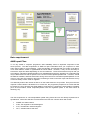
AgroMetShell (AMS) provides a toolbox for agrometeorological crop monitoring and forecasting. The
current visual menu offers easy access to some of the most often used functions.
The program includes a database that holds all the weather, climate and crop data needed to analyse
weather impact on crops. Data can be input into the database using a variety of options, for instance,
they can be typed in from the keyboard, read from WINDISP format images or imported from ASCII
files. Number of operations can be performed on the database, such as making backups or flushing
the database.
The core of the program is the FAO Crop Specific Soil Water Balance. The basic of this soil water
balance calculation is given in the file CSSWB.doc and in the watersatisfactionindex.xls
FAO Crop Specific Soil Water Balance can be operated in monitoring mode or in risk analysis mode.
The first is an analysis for one growing season covering many stations in a specific area, usually a
country or a province in a country. The second (risk analysis) covers the same type of analysis for one
station only, but over many years.
The FAO Crop Specific Soil Water Balance produces a number of outputs: water balance variables,
such as soil moisture, actual evapotranspiration over the vegetative phase or the water stress at
flowering, etc. They can be mapped separately for crop monitoring. For crop forecasting, the water
balance variables are normally averaged over administrative areas and then compared with crop
yields through multiple regression to derive a Yield Function that in turn can be used to estimate
yields.
In addition to the FAO Crop Specific Soil Water Balance, the program proposes many other useful
tools, for instance the calculation of rainfall probabilities, spatial interpolation tools and the
determination of growing season characteristics based on climatological parameters.
1
Data requirement
AMS input Files
To run any model or computer programme, data availability forms an important component of the
whole process. The data requirement of AMS are quite reasonable when you compare it to other
heavy duty models for crop simulation. There are basically 10 input files that one needs, to be able to
run a water balance model in AgroMetShell as shown below. However, it may not be necessary to
have all the input files listed depending on the circumstances. These circumstances may be that you
are unable to calculate evapotranspiration on a dekadal basis and hence preparing an evaporation file
may be difficult and one has no option but to use the normal evapotranspiration file. However, should
the data be available, AMS has extra tools among which the tool to calculate evapotranspiration is one
of them. There are also instances where the monitoring is done for rain-fed crops and therefore it may
not be necessary to have a file on irrigation.
This basically reduces the number of files to run the water balance to 5 input files. Every time the user
requests a water balance calculation to be carried out, the programme prepares a set of files that will
be read by the Crop Specific Soil Water Balance programme to compute the water balance variables
(such as soil moisture, actual evapotranspiration over the vegetative phase or the water stress at
flowering, etc).
The files required are in comma-separated quoted string format and can be directly imported into a
spreadsheet. All the files will have common data in the first four columns which will contain:
•
•
•
•
"NAME", the station Name
"LON", the longitude in decimal degrees
"LAT", the latitude in decimal degrees
"ALT", elevation above sea level
2
To run a crop specific water balance calculation, one needs the following files:
Input 1: Country Name_2003_Crop_Dekad_Input.dat
The file contains a summary of the parameters used to run the water balance, including the following:
•
•
•
•
•
•
•
•
"WHC", soil water holding capacity
"Efrain", effective rain (a percentage by which
actual rain is multiplied to assess actual water
supply. Usually Efrain<100% on slopes and
Efrain>100% in low lying areas
"Crop-ID#", the internal identification number of
the crop
"Cycle", the cycle length in dekads
"Pldek", the planting dekad, a value between 1
and 36
"Irrig", the type of irrigation (1=yes, 0=no and
2=automatic)
"BundH", the height of the bund, for irrigated
crops
"k1","k2","k3","k4"…. Up to the value
corresponding to the last dekad of the cycle, crop coefficients KCP
Input 2 and 3: Country Name_2003_Rain_Dekad_Input.dat
Country Name_2004_Rain_Dekad_Input.dat
The two files have actual rainfall for two consecutive years, as it often occurs that the crop is planted in
one year and harvested in the following one. This kind of situation is what happens with winter crops
in Belgium and with most crops in southern Africa where rainfall commences in September/October of
one year and terminates in April/May of the following year. However, in situations where an
agricultural season falls within a calendar year which is the case for spring wheat in Armenia, AMS will
still work.
Input 4 and 5: Country Name_2003_Irrigation_Dekad_Input.dat
Country Name_2004_Irrigation_Dekad_Input.dat
The files contain actual values only if they have actually been provided. In monitoring rain-fed crops,
these failes are not necessary.
Input 6 and 7: Country Name_2003_PET_Dekad_Input.dat
Country Name_2004_PET_Dekad_Input.dat
The two files have actual potential evapotranspiration for two consecutive years, as it often occurs that
the crop is planted in one year and harvested in the following one. Evapotranspiration plays an
important role in the water balance as it represents the atmospheric demand. If evapotranspiration is
not available, it has to be calculated from other meteorological variables
Input 8 to 10: Country Name _Normal_Rain_Dekad_Input.dat
Country Name _Normal_PET_Dekad_Input.dat
Country Name _Normal_Irrigation_Dekad_Input.dat
The files contain normal rainfall, PET and Irrigation. The data from these files is utilized if the actual
data is missing in the input files.
3
AMS Output Files
The programme generates 18 output files. It is not necessary that the user knows the details of the
structure of those files, but with experience you may feel the need to carry out some non-standard
analyses, in which case the information below will be of help. The names of output files are assigned
automatically to the files based on the year, file list, type of data (input or output, daily or by dekad,
actual or normal data) so that the file contents should be easy to determine. In addition, the first line of
each file has a description of the data. Missing values in the files are usually coded as –999. All input
and output files with DAT extensions follow the same “FAO format”.
Two types of output files are produced. Those with extension TXT (text) provide some descriptive
material about the crop monitoring exercise, while those with DAT extensions are in comma-separated
quoted string data files used by other options of the programme, for instance many of the options
under the Tools menu.
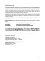
Output 1 and 2: TXT (text) output files, Country Name _2004_Details_Dekad_Output.txt and
Output_Comments.txt
Output_Comments.txt simply lists information about the files as they are processed. An example
follows:
AM-ARENI
AM-MERDZAVAN
AM-GYUMRI
AM-YEREVAN
: No calculations done: Missing Planting Dekad
: No calculations done: Missing Water Holding Capacity
: Water balance calculated successfully
: No calculations done: Missing Planting Dekad
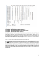
The second file (Country Name_2004_Details_Dekad_Output.txt) contains the full details about the
water balance. An example is given below. The abbreviations have the following meaning: NOR is
normal rainfall, ACT is actual rainfall, WRK stands for “working” rainfall, i.e. WRK=ACT*EfRain/100 if
Act is available, otherwise WRK=NOR*EfRain/100, Irr is the irrigation amount if any, PET is the
potential evapotranspiration while WR (the water requirement) is the product of KCR*PET. AvW is the
crop available water, S/D stands for water Surplus or Deficit and, finally INDEX is the Water
satisfaction index, the percentage of the crop water requirements that has actually been met. The end
of the table lists actual evapotranspiration, water surplus and deficit by phenological phases:
Station number: 40/ Crop 14
Station Name: STATION000040 (Elevation:-999 m)
Crop type: Potato
Cycle length: 13 dekads (C)
Total water requirements: 389 mm (TWR)
Normal water requirements: 319 mm (TWRNor)
Planting dekad: 13
(P)
Maximum soil water storage: 100 mm
(H or WHC)
Effective/Total rain: 100 %
(E or EfR%)
Irrigation applied: Automatic
Bund Height: 50 mm
(BUH)
Pre-season Kcr : 0.30
4
Output 3 to 6: DAT output files,
Country Name _1998_WaterSatisfactionIndex_Dekad_Output.dat,
Country Name _1998_WaterStorage_Dekad_Output.dat,
Country Name _1998_WaterSurplusDeficit_Dekad_Output.dat and
Country Name _1998_ActualPET_Dekad_Output.dat
The files are "monitoring-oriented" as they contain sequences of several dekad values for display and
inter-station comparisons. They respectively contain water satisfaction index values, soil moisture,
water surplus or deficit and actual evapotranspiration, dekad by dekad, for all the stations in the list.
Note that dekads are crop dekads (from 1 to cycle length). Values beyond cycle length are coded with the
default value for missing data. D1, D2...D36 are the dekad numbers in crop dekads (i.e. planting dekad is
1 and the last values corresponds to C, the cycle length).
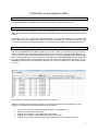
Output 7: Country Name _1998_RangelandIndex_Dekad_Output.dat
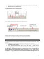
The "rangeland-index" (RI) is the classic FAO water satisfaction index computed for periods of 5 dekads,
with normal evapotranspiration kept at potential level (KCR=1) and an assumed WHC of 50 mm. Similar
to moving averages, the value assigned to a dekad corresponds to the five-dekad period centred about
that dekad. Thus 3 for dekads 1 to 5, 4 for dekads 2 to 6... The rangeland index, when plotted over time,
assumes a smoothed aspect, as shown in the figure below that compares "rangeland index" (RI) with
rainfall (mm) in Msabaha (Kenya) in 1984. RI is associated with crop phenology. Based on local
experience, there is usually a rather good association between planting and the RI. For instance, in
Tanzania, it was found that the planting of millet usually occurs when the rising RI curve crosses the 0.4
(40%) threshold.
5
The RI is computed using actual rain (not "working rain" as described above, i.e. future values are coded
as missing and not taken as their normal).
The dekads when the RI curve passes the 30 to 70% thresholds is given in the second text output file
(Country Name _1991_Details_Dekad_Output.txt above).
Output 8: Country Name _1991_Summary_Dekad_Output.dat
The "summary" output file is certainly the most useful, as it lists the parameters which are likely to be
used for further processing and analysis, in particular for developing yield models for yield estimation and
crop forecasting. In addition to station ID, longitude (X) and latitude (Y), %AVAIL (percent of actual data
used in the calculations) and Z (elevation) the variables listed in the "summary" are the following:
H and WHCi, the soil Water Holding Capacity, and its initial value, respectively;
EfR%, the ratio between effective and actual total and rain, in percent (Efrain, see
above);
P, the planting dekad (1-36);
C, the length of the crop cycle (dekads);
TWR, total water requirements in mm;
Indx, IndxNor and IndxLatest, FAO soil water satisfaction index, in % of requirements,
respectively actual, normal and "last" values. "Actual" corresponds to the
value expected at the end of the cycle, "normal" is the end-of-cycle index
computed with normal rain and PET, all other parameters being those from the
crop file; the "last" value is that of the last dekad for which actual data are
1[1]
available ( );
WEXi, WEXv, WEXf, WEXr, WEXt, water excess over the phenological phases
described as initial, vegetative, flowering, harvest and the whole cycle (sum of
previous values)
WDEFi, WDEFv, WDEFf, WDEFr, WDEFt, water deficit over the phenological phases
and the value totalled over the growing cycle
ETAi, ETAv, ETAf, ETAr, ETAt, actual evapotranspiration
phases and the value totalled over the growing cycle
over the phenological
1[1]
If there are no actual data available (in which case "actual" and "normal" are identical), then the "last" index is coded
as missing.
6
ETA: actual crop evapotranspiration (i.e. actual crop water consumption), a factor
directly related with crop yield;
%Av, ("available") the percentage of actual rainfall data used for the calculations (the
rest being assumed to be "normal")
Cr1a to Cr4a and Cr1n to Cr4n (for "Crossing" and "Normal Crossing") indicate the dates
(dekads) when the rangeland index (see above) crosses the 0.4*PET line. The dekads
given in the file can be used to map the beginning of the actual (current) season (Cr1 to
Cr4) and the normal beginning (NCr1 to NCr4). In areas with only one rainfall peak, there
is only one "normal" start, but there are two in bimodal rainfall areas. In marginal areas,
where rainfall is very close to 40% of PET, there may be more than one "start" even in
areas with uni-modal rainfall. The actual starts may be more than the "normal starts",
particularly in the not so rare event of "false starts" when rain decreases again after a first
start: in the field, farmers must frequently replant when this happens.
7
EXERCISE into AgrometShell (AMS)
AMS installation
The “Agrometshell.exe” installation file is given in the beginning of the training course.
AMS configuration
AMS needs first to be configured in order to be adapted to your own work. This concerns the ascii
editor, the boundary file (world.bna by default) that should be Armenia and the image file (world.img by
default).
In the EDIT menu, go to “GENERAL CONFIGURATION” and modify the default values. Select a text
(ASCII) editor in your computer, select the boundary file of Armenia and an image of Armenia. Finally
in order to have this new configuration active, it is adviced to restart AMS. So, quit AMS and restart it.
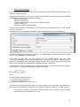
STATIONS LIST
The command MANAGE STATIONLIST allows you to either create a list of stations that you will use to
make a monitoring run or to load an existing list that you intend to use in running a water balance. To
create a new list, select Create new list and then provide a name under Specify a new name for the
list. To load an existing list, click on the down arrow and select Load existing list and this will provide
you with an option to select an appropriate list. Once the name of the list has been provided, you may
click OK and the following screen appears allowing you to select the stations you want to be included
in the list.
In this exercise, create a new list of stations and call it “Armenia”.
Stations can either be taken from the <Base List> if already included or entered directly into this
window. For all stations the following attributes can be defined:
•
•
•
•
•
ID. This is a code that uniquely identifies the station in the database
Name. This is the name of the station.
Latitude and Longitude : the coordinates of the station.
Altitude. The elevation of the station (height above sea-level).
Country and Country Code. The name of the country in which the station is located.
8
•
•
Administrative levels. The administrative level 1 and 2 within a country. E.G. Province and
District.
Three extra attributes (to be filled at will).
The buttons at the top have the following functions:
Then, a number of buttons provide other ways to manipulate the list:
Pressing <OK> will save the list. Pressing <Cancel> will cancel all changes.
In this exercise, you are asked to enter directly 5 Armenian weather stations !
DATA INPUT
This exercise will serve for the preparation of input data for the water balance calculation that will be
done later.
The FAO methodology for the water balance calculation is based on two main assumptions :
1. the ten-daily time step is sufficient to estimate with an acceptable accuracy the water balance
for agrometeorological purposes;
2. Normal potential evapotranspiration (PET) can be used instead of actual reference
evapotranspiration (see notes of Frere and Popov (1979) for more explanations) when actual
PET is not available.
The water balance will calculate the evolution of the soil water content according to rainfall input and
deep percolation and actual evapotranspiration output. This calculation is run at a 10-daily time step.
Percolation may also be calculated but this has no operational meaning for an agrometeorologist and
will be skipped here. Therefore we will need dekadal values of both ET0 and rainfall data.
9
1. Introduction of Normal data
The exercise is done with data from Armenia. Normal monthly data of 9 rainfall stations and normal
monthly values of Mean Temp of 8 stations are available into the FAOCLIM database. A rapid
presentation of this database will be done by B. Tychon.
All the data available were saved in 2 files named rainfallnormal.dat and Meantempnorm.dat. Open
these files and confirm that the data do correspond with reality.
Then, with Excel spreadsheet, modify the format of the 3 files in order to have
Column A : station name
Column B : station ID
Column C : Longitude
Column D : Latitude
Column E : Altitude
Next columns : Monthly values from January to December.
Delete all the other columns.
Save these files in CSV format (comma separator) with the following names:
- rainnorm.csv
- meantemp.csv.
Once you have saved these data, go into AMS and try to import these Temp and Rainfall normal data
into AMS using the ‘import’ button (or the menu Database/import/from ascii file) and replying to the
different steps requested by AMS.
Be careful ! Verify that the station names are exactly the same as those you already introduced into
the database before importing them ! Any spell mistakes will lead to the building of a new ‘wrong’
station and you will have to restart the import procedure.
The importation procedure will be presented during the course on some examples by B. Tychon
If the importation runs well, you should see the results in the menu DATABASE/DATA INVENTORY.
Please check it.
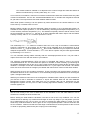
You can see the results of the new data on a map in the menu DATABASE/MAP. Try for example to
see the rainfall values on the map for the month of August. Choose also another month with dryer
conditions.
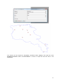
There exists two ways to do maps. The first one will show stations values on a map. You can have this
presentation by applying the following procedure : DATABASE/MAP. The example here is for normal
rainfall in August.
10
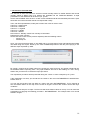
The second one will request an interpolation procedure before mapping. First open the menu
INTERPOLATE/MAKE INPUT FILE/DATABASE to create an output file that will serve in the
interpolation.
11
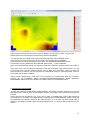
Next, do the interpolation with the following command : INTERPOLATE/INVERSE DISTANCE
You should have such map.
12
These maps can be saved to be used in report or bulletin you may have to write. They have the
windisp format and can therefore be improved for report presentations.
You can also see your rainfall values using the report button into the DATABASE menu.
In the first line you must say in which list you want to get the data (Row): ARMENIA.
In the second line must be defined the Type of data : for example Normal Monthly values.
The third line is for the Parameter name (Rainfall, Wind speed,…). Choose Rainfall.
Then you must write which period you want to be put into the report (for example month 8 to month 11
).
Once this is done, you can add this information in the report using the “add column” button. You can
do it several times, choosing different column ‘types of data’ and ‘parameters’. When you have the
wished number of columns, you can send this to a Worksheet (excel) or a Wordprocessor (word) or
more simply into an ascii file Editor.
These monthly Normal data need now to be converted into 10-daily data using the conversion
process into the DATABASE MENU /CALCULATE/NORMALS/DEKADAL FROM MONTHLY
PROCEDURE. Please verify the results into the Data inventory in the Database menu.
2. Introduction of actual data
You can then introduce actual rainfall, relative humidity, wind speed, sunshine duration, amx and min
temperature from 1998 to 2010 for all available stations. The station choice will be done during the
exercise.
These data will be provided by you. They can be daily or dekadal data. These data should be
converted into an ascii files (csv format) and then imported into the AMS database. Please check that
the importation runs well by looking at the Data Inventory. You can also see these actual data on
graphs by selecting the ‘Graph’ option into the Database menu. Try to see 3 stations together on your
screen !
13
3. ET0 or PET calculation
This second exercise will concern introduction of actual daily weather data with the calculation of the
reference evapotranspiration.
We will use data introduced in the previous step into the database. PET or ET0 can only be calculated
if the following meteorological variables are available :
- Minimum Temperature
- Maximum Temperature
- Average relative humidity or max and min relative humidity
- Average wind speed
- Sunshine duration or Global radiation
If all this data is available in the database, which is the case in this training session, you can proceed
to the PET calculation.
Calculate the ET0 using the formula available in AMS (DATABASE/CALCULATE/FORMULA)
ET0 will be calculated automatically and saved in the AMS database. Check the results in the data
inventory. (DATABASE/DATA INVENTORY).
If the data are daily data, you can convert them into dekadal values using the option
CALCULATE/AGREGATE into the DATABASE menu. This option will tranform automatically your
daily values into dekadal and monthly data. Apply this process for all stations into the ArmeniaTraining
list to convert daily data into dekadal date and dekadal data into monthly data.
If one of the meteo input data for the ET0 calculation is missing, it has to be estimated. For example,
solar radiation, Rs, can be estimated with the Hargreaves formula :
where
-2
-1
Ra extraterrestrial radiation [MJ m d ],
Tmax maximum air temperature [°C],
Tmin minimum air temperature [°C],
-0.5
kRs adjustment coefficient (0.16.. 0.19) [°C ].
The square root of the temperature difference is closely related to the existing daily solar radiation in a
given location. The adjustment coefficient kRs is empirical and differs for 'interior' or 'coastal' regions:
• for 'interior' locations, where land mass dominates and air masses are not strongly
influenced by a large water body, kRs ≅ 0.16;
14
• for 'coastal' locations, situated on or adjacent to the coast of a large land mass and where air
masses are influenced by a nearby water body, kRs ≅ 0.19.
In our exercise, one stations, Areni has no sunshine measurement and these measurements only start
in 2004 for Merdzavan. Use the file “extraterrestrialradiation.xls” to calculate the Hargreaves formula
for year 2007. Then import these new solar radiation data into AMS.
When wind speed is missing it can be replaced by values observed in the closest stations or in the
worse case by a constant value of 2 m/s.
Missing relative humdity may also be estimated if data are lacking or are of questionable quality, an
estimate of actual vapour pressure, ea, can be obtained by assuming that dewpoint temperature (Tdew)
is near the daily minimum temperature (Tmin). This statement implicitly assumes that at sunrise, when
the air temperature is close to Tmin, that the air is nearly saturated with water vapour and the relative
humidity is nearly 100%. If Tmin is used to represent Tdew then:
The relationship Tdew ≈ Tmin holds for locations where the cover crop of the station is well watered.
However, particularly for arid regions, the air might not be saturated when its temperature is at its
minimum. Hence, Tmin might be greater than Tdew and a further calibration may be required to estimate
dewpoint temperatures. In these situations, "Tmin" in the above equation may be better approximated
by subtracting 2-3 °C from Tmin.
You can calculate missing relative humidity with the actualvaporpressure.xls file. You just need to
replace Tmax and Tmin with the values of your stations.
The reference evapotranspiration (ET0) can also be calculated with AMS by using in the menu
TOOLS/POTENTIAL ET. You have there two options to calculate it, either manually, by introducing all
the weather parameters day by day or by using a FAO format file that contains all the necessary input
variables. A example of such file is ET0solutionmultan.csv. Try this option with that file ! Be careful!
Never use at the same time an average input variable with max and min values of that same variable.
AMS can also serve for the encoding procedures. These procedures may be activated by clicking on
the different buttons on the ‘visual menu’ or more classically through the Database menu choosing the
option ‘manage weather data’.
AMS may be used as a basic tool for the management of weather data. It will be you who will decide in
your Service if this is worthwile to introduce or import the weather data into this new Database
Management System. Please note finally that not only weather data can be introduced into the
Management System but any kind of data including agricultural statistics, food prices, fertilizer
amounts applied, etc.
WATER BALANCE
We are now moving to the core of AMS which is the calculation of the soil water balance. This is
located in the middle part of the visual menu.
Before starting the water balance calculation, lets have a look at the crop coefficient. You can use
default values for defining crop coefficient and length of each crop stage or you may define your own
set of parameters for the crop on which you want to simulate the water balance. Create your own
wheat crop coefficient based on what is given in the “crop evapotranspiration” manual. Save this new
set as ‘armenian’. Please note that the initial stage is subdivised into several periods to take account
on winter crops passing winter and a part of spring in this initial stage.
15
You can start by clicking on the ‘New run’ button. Enter the name you want to give to this run. Choose
the list with the stations where you want the water balance to be done. Select the starting year for the
run and give the name of the crop you want to simulate. For this exercise we will call this run
“Armenia-wheat_2009”. We’ll work with the 3 stations of the 3 provinces with 2008 as starting year and
we’ll do the simulation for wheat.
After validation, a table to fill will be presented. You will have to choose for each station in the selected
list,
- the dekad of sowing,
- the cycle length,
- the water holding capacity,
- the percentage of rainfall that will be effective for the soil-plant system,
- the pre-season coefficient that represents the amount of water lost by bare soil and weeds
before the sowing date when compared to the reference evapotranspiration,
- the irrigation application : 3 possible options : no irrigation (rainfed crops), irrigation
applications calculated by AMS for keeping the Water Satisfaction Index to 100% during all
the crop cycle or irrigation applications according to information provided as input data for the
different stations. In this last case, input data should be incoded into the AMS database using
the ‘actual 10-day data’ button and choosing the parameter ‘irrigation’.
- The bund height of the plot when irrigation consists on plot water ponding.
This table can be filled record by record. In this particular exercise, we will use the button that will set
the same value for all the column. Values for the different parameters of this table will be choosen
during the course. Note that in all the table, a cell, a line or a column may be selected as the default
one if you activate one of the 4 ‘set default’ buttons above the table. Check it.
You may then either just save this set of parameters or save and run the water balance. Select this
last option and run the water balance model. This run a water balance for all stations with actual
dekadal rainfall and actual dekadal potential evapotranspiration. This means that you must absolutely
have these two informations if you want AMS to calculate the water balance. When data are missing,
they are replaced by normal data. Check it by doing the same simulation but this time for the
campaign 2003. This will allow to simulate what happens when actual data are missing (we have no
ET0 data in 2003 for Merdzavan). What happens with the output ? Are there problems with some
stations ? Can you explain why ?
All the output files of the waterbalance calculation are available in the output directory you selected in
the running process. Go to this directory and open all the output files et check that you understand
their content.
In a first step, run the water balance calculation with no irrigation application (Option 0). During the
run, all the results are saved in different files. The definition of each output variable is given in the
AMS user manual. Take ten minutes to read it carrefuly.
You clearly see that the Water Satisfaction Index in Armenia when starting crop in the first dekad of
May fall to very bad values in some districts. This simply means that, in these areas, acceptable yields
may only be obtained with irrigation or in soil with very high water holding capacity. The second option
(Option 2) for the irrigation application may then be applied. AMS will calculate the amount of water to
apply on the field to keep the WSI to 100%. Compare the amount of ETA of the two different
simulations. Do it for the 3 stations.
Finally, use your own data of irrigation schedule according to your personal experience or the one
from your colleagues (Option 1) and apply it to the 3 stations.
Make an image of the water balance results using WATER BALANCE\MAKE IMAGE FROM
RESULTS. This option of AMS allows you to draw maps of all the outputs of the summary output file,
the most important output file that gives the essential information. In the present case, draw a map of
the ETA(total), WSI (Last index) and Water deficit at flowering stage.
Once you have calculated the waterbalance for 2004, do it for the different years you have in your
database, especially for the period where agricultural statistics are available.
16
RISK ANALYSIS RUN
This option is quite similar to the water balance but this time, instead of runing the water balance for a
particular year on a set of weather stations, we will calculate the water balance for several years on a
unique selected weather station. The objective is the analyse of the evolution of the water stress on a
great number of years in order to specify for each station the risk to have a water stress problem.
Based on this risk evaluation, the farmer will decide on the strategy to fight against the stress (crop
variety, crop practices, type of sowing (dry or wet), irrigation,…).
We can do the exercise on the Areni station in Aremia where data from one station are available for 12
years (1998-2010). Run it using the new run ‘button into the risk analysis window or through the menu
‘WATER BALANCE/RISK ANALYSIS RUN/NEW.
Analyse the results. What are the risks to have high water stress around this station ? What is the
average amount of irrigation water necessary in 2004 to keep the crop in optimal growth conditions?
17