Download this tutorial

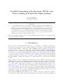
Parallel Computing with Bayesian MCMC and
Data Cloning in R with the dclone package
Péter Sólymos
University of Alberta
Abstract
The dclone R package provides parallel computing features for Bayesian MCMC computations and the use of the data cloning algorithm. Parallelization can be achieved by
running independent parallel MCMC chains or by partitioning the problem into subsets.
Size balancing is introduced as a simple workload optimization algorithm applicable when
processing time for the pieces differ significantly. The speed-up with parallel computing
infrastructure can facilitate the analysis of larger data and complex hierarchical models
building upon commoly available Bayesian software.
Keywords: Bayesian statistics, data cloning, maximum likelihood inference, generalized linear
models, R, parallel computing.
1. Introduction
Large data and complex hierarchical models pose a challenge to statistical computations.
For this end researchers often use parallel computing, especially for “embarassingly parallel
problems” such as Markov chain Monte Carlo (MCMC) methods. R (R Development Core
Team 2010) is an open source software and environment for statistical computing and has
interfaces for most commonly used Bayesian software (JAGS, Plummer (2010); WinBUGS,
Spiegelhalter et al. (2003); and OpenBUGS Spiegelhalter et al. (2007)). R also has capabilities
to exploit capacity of multi-core machines or idle computers in a network through various
contributed packages (Schmidberger et al. 2009). R is thus a suitable platform for parallelizing
Bayesian MCMC computations, which is not a built-in feature in commonly used Bayesian
software.
Data cloning is a global optimization algorithm that exploits Markov chain Monte Carlo
(MCMC) methods used in the Bayesian statistical framework while providing valid frequentist inferences such as the maximum likelihood estimates and their standard errors (Lele
et al. 2007, 2010). This approach enables to fit complex hierarchical models (Lele et al.
2007; Ponciano et al. 2009) and helps in studying parameter identifiability issues (Lele et al.
2010; Sólymos 2010), but comes with a price in processing time that increases with the number of clones by repeating the same data many times, thus increasing graph dimensions in
the Bayesian software used. Again, parallelization naturally follows as a reply to the often
demanding computational requirements of data cloning.
The R package dclone (Sólymos 2010) provide convenience functions for Bayesian computations and data cloning. The package also has functions for parallel computations, building on
2
Parallel computing with MCMC and data cloning
the parallel computing infrastructure provided by the snow package (Tierney et al. 2010). In
this paper I present best practices for parallel Bayesian computations in R, describe how the
wrapper functions in the dclone package work, demonstrate how computing time can improve
by these functions and how parallelization can be effectively optimized.
2. Bayesian example
We will use the seeds example from the WinBUGS Manual Vol. I. (Spiegelhalter et al. 2003)
based on Table 3 of Crowder (1978). The experiment concerns the proportion of seeds that
germinated on each of 21 plates arranged according to a 2 × 2 factorial layout by seed (x1i )
and type of root extract (x2i ). The data are the number of germinated (ri ) and the total
number of seeds (ni ) on the ith plate, i = 1, . . . , N :
R> source("http://dcr.r-forge.r-project.org/examples/seeds.R")
R> str(dat <- seeds$data)
List of 5
$ N : num
$ r : num
$ n : num
$ x1: num
$ x2: num
21
[1:21]
[1:21]
[1:21]
[1:21]
10 23
39 62
0 0 0
0 0 0
23 26
81 51
0 0 0
0 0 1
17 5 53
39 6 74
0 0 0 0
1 1 1 1
55 32 46 ...
72 51 79 ...
...
...
The Bayesian model is random effects logistic, allowing for overdispersion:
ri ∼ Binomial(pi , ni )
logit(pi ) = α0 + α1 x1i + α2 x2i + α12 x1i x2i + bi
bi ∼ Normal(0, σ 2 ),
where pi is the probability of germination on the ith plate, and α0 , α1 , α2 , α12 and precision
parameter τ = 1/σ 2 are given independent noninformative priors. The corresponding BUGS
model is:
R> (model <- seeds$model)
function() {
alpha0 ~ dnorm(0.0,1.0E-6);
# intercept
alpha1 ~ dnorm(0.0,1.0E-6);
# seed coeff
alpha2 ~ dnorm(0.0,1.0E-6);
# extract coeff
alpha12 ~ dnorm(0.0,1.0E-6);
# intercept
tau
~ dgamma(1.0E-3,1.0E-3); # 1/sigma^2
sigma <- 1.0/sqrt(tau);
for (i in 1:N) {
b[i]
~ dnorm(0.0,tau);
logit(p[i]) <- alpha0 + alpha1*x1[i] + alpha2*x2[i] +
alpha12*x1[i]*x2[i] + b[i];
r[i]
~ dbin(p[i],n[i]);
}
}
Initial values are taken from the WinBUGS manual
Péter Sólymos
3
R> str(inits <- seeds$inits)
List of 5
$ tau
:
$ alpha0 :
$ alpha1 :
$ alpha2 :
$ alpha12:
num
num
num
num
num
1
0
0
0
0
We are using the following settings (n.adapt + n.update = burn-in iterations, n.iter is the
number of samples taken from the posterior distribution, thin is the thinning value, n.chains
is the number of chains used) for fitting the JAGS model and monitoring the parameters in
params:
R>
R>
R>
R>
R>
R>
n.adapt <- 1000
n.update <- 1000
n.iter <- 3000
thin <- 10
n.chains <- 3
params <- c("alpha0", "alpha1", "alpha2", "alpha12", "sigma")
The full Bayesian results can be obtained via JAGS as
R> m <- jags.fit(data = dat, params = params, model = model,
+
inits = inits, n.adapt = n.adapt, n.update = n.update,
+
n.iter = n.iter, thin = thin, n.chains = n.chains)
3. Parallel MCMC chains
Markov chain Monte Carlo (MCMC) methods represent an “embarassingly parallel problem”
(Rossini et al. 2003; Schmidberger et al. 2009) and efforts are being made to enable effective
parallel computing techniques for Bayesian statistics (Wilkinson 2005), but popular software
for fitting graphical models using some dialect of the BUGS language (e.g. WinBUGS, OpenBUGS, JAGS) do not yet come with a built in facility for enabling parallel computations (see
critique for Lunn et al. (2009)).
WinBUGS has been criticized that the indepencence of parallel chains cannot be guaranteed via
setting random number generator (RNG) seed (Wilkinson 2005). Consequently, parallelizing
approaches built on WinBUGS (e.g. GridBUGS Girgis et al. (2007); or bugsparallel Metrum
Institute (2010)) are not best suited for all types of parallel Bayesian computations (e.g. those
are best suited for batch processing, but not for generating truly independent chains). One
might argue that the return times of RNG algorithms are large enough to be safe to use a
different seeds approach, but this approach might be risky for long chains as parallel streams
might have some overlap, and parts of the sequences might not be independent (see Wilkinson
(2005) for discussion). Also, using proper parallel RNG of the rlecuyer package (Sevcikova and
Rossini 2009) used in the R session to ensure independence of initial values or random seeds
will not guarantee chain independence outside of R (e.g. this is the case in the bugsparallel
project according to its source code).
Random numbers for initialization in JAGS are defined by the type and seed of the RNG, and
currently there are four different types of RNGs available (base::Wichmann-Hill, base::-
4
Parallel computing with MCMC and data cloning
Marsaglia-Multicarry, base::Super-Duper, base::Mersenne-Twister). The model initialization by default uses different RNG types for up to four chains, which naturally leads to
safe parallelization because these can represent independent streams on each processor.
Now let us fit the model by using MCMC chains computed on parallel workers. We use three
workers (one worker for each MCMC chain, the worker type we use here is “socket”, but type
can be anything else accepted by the snow package, such as "PVM", "MPI", and "NWS"):
R> library(snow)
R> cl <- makeCluster(3, type = "SOCK")
Because MCMC computations (except for generating user supplied initial values) are done
outside of R, we just have to ensure that model initialization is done properly and initial
values contain different .RNG.state and .RNG.name values. Up to four chains (JAGS has 4
RNG types) this can be most easily achieved by
R> inits2 <- jags.fit(dat, params, model, inits, n.chains,
+
n.adapt = 0, n.update = 0, n.iter = 0)$state(internal = TRUE)
Note that this initialization might represent some overhead especially for models with many
latent nodes, but this is the most secure way of ensuring the independence of MCMC chains.
We have to load the dclone package on the workers and set a common working directory
where the model file can be found (a single model file is used to avoid multiple read/write
requests):
R> clusterEvalQ(cl, library(dclone))
R> clusterEvalQ(cl, setwd(getwd()))
R> filename <- write.jags.model(model)
Using a common file is preferred when the mamory is shared (e.g. for SOCK cluster type). If
computations are made on coputing grid or cluster without shared memory, each machine
needs a model file written onto the hard drive. For this, one can use the write.jags.model
function with argument overwite = TRUE to ensure all worker has the same model file name.
In this case, the name of the model file can be provided as a character vector in subsequent
steps.
The next step is to distribute the data to the workers
R> cldata <- list(data=dat, params=params, model=filename, inits=inits2)
R> clusterExport(cl, "cldata")
and create a function that will be evaluated on each worker
R> jagsparallel <- function(i, ...)
{
+
jags.fit(data = cldata$data, params = cldata$params, model = cldata$model,
+
inits = cldata$inits[[i]], n.chains = 1, updated.model = FALSE, ...)
+
}
Now we can use the parLapply function of the snow package and then clean up the model
file from the hard drive
R> res <- parLapply(cl, 1:n.chains, jagsparallel,
+
n.adapt = n.adapt, n.update = n.update, n.iter = n.iter, thin = thin)
R> res <- as.mcmc.list(lapply(res, as.mcmc))
R> clean.jags.model(filename)
Péter Sólymos
5
The jags.parfit function in the dclone package is a wrapper for this process, here we can
use the model function instead of a model file
R> m2 <- jags.parfit(cl, data = dat, params = params, model = model,
+
inits = inits, n.adapt = n.adapt, n.update = n.update,
+
n.iter = n.iter, thin = thin, n.chains = n.chains)
R> stopCluster(cl)
The jags.parfit is the parallel counterpart of the jags.fit function. It internally uses
the snowWrapper function because clusterExport exports objects from the global environment and not from its child environments (i.e. from inside the jags.parfit function). The
snowWrapper function takes care of name clashes and also can be used to set the parallel random number generation type via the clusterSetupRNG function of snow. The dclone package
can use the L’Ecuyer’s RNG (L’Ecuyer et al. 2002) ("RNGstream", requires the rlecuyer package, Sevcikova and Rossini (2009)) or "SPRNG" (requires the rsprng package, Li (2010)). The
type of parallel RNG can be set up by the dcoptions function and by default it is "none"
(not setting up RNG on the workers). Setting the parallel RNG can be important when using
random numbers as initial values supplied as function, so the function is evaluated on the
workers. To set the RNG type, we use
R> dcoptions(RNG = "RNGstream")
R> dcoptions()$RNG
[1] "RNGstream"
Table 1 shows different ways of providing initial values. Besides setting up RNGs, we might
have to export objects to the workers using the clusterExport function of the snow package
if inits contains a reference to objects defined in the global environment.
4. Parallel data cloning
Data cloning uses MCMC methods to calculate the posterior distribution of the model parameters conditional on the data. If the number of clones (k) is large enough, the mean of the
posterior distribution is the maximum likelihood estimate and k times the posterior variance
is the corresponding asymptotic variance of the maximum likelihood estimate (Lele et al.
2007, 2010). But there is no universal number of clones that is needed to reach convergence,
so the number of clones has to be determined empirically by using e.g. the dctable and dcdiag functions provided by the dclone package (Sólymos 2010). For this, we have to fit the
same model with the different number of clones of the data, and check if the variances of the
parameters are going to zero (Lele et al. 2010). Fitting the model with number of clones, say
(1, 2, 5, 10, 25), means that we have to fit the model five times. Without parallelization, we
can use subsequent calls of the jags.fit function with different data sets corresponding to
different number of clones, or use the dc.fit wrapper function of the dclone R package.
Parallelization can happen in two ways: (1) we parallelize the computation of the MCMC
chains (ususally we use more than one chain to check proper mixing behaviour of the chains);
or (2) we split the problem into subsets and run the subsets on different worker of the parallel computing environment. The first type of parallelization can be addressed by multiple
calls to the jags.parfit function. The second type of parallelization is implemented in the
dc.parfit function that is the parallelized version of the function dc.fit.
6
Parallel computing with MCMC and data cloning
inits
NULL
Self contained named
list
Named list with references to global environment
Self contained function
Function using random
numbers
Fuction with references
to global environment
Effect
Initial values automatically
generated with RNG type and
seed
inits used, RNG type and
seed generated if missing
ditto
Notes for parallel execution
None
Function used to generate
inits, RNG type and seed
generated if missing
ditto
None
ditto
None
Objects must be exported by
clusterExport()
Parallel RNG should be set by
dcoptions() or clusterSetupRNG()
Objects must be exported by
clusterExport()
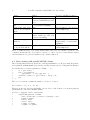
Table 1: Different ways of providing initial values and notes for parallel executions. Self
contained means that the object has no reference to other objects or environments, neither
random numbers are generated within a self contained function.
4.1. Data cloning with parallel MCMC chains
The following simple function allows us to switch parallelization on/off (by setting the parallel argument as TRUE/FALSE, respectively), and also measure the processing time in minutes:
R> timerfitfun <- function(parallel = FALSE, ...) {
+
t0 <- proc.time()
+
mod <- if (parallel)
+
jags.parfit(...) else jags.fit(...)
+
attr(mod, "timer") <- (proc.time() - t0)[3] / 60
+
mod
+
}
The vector n.clones contains the number of clones to be used:
R> n.clones <- c(1, 2, 5, 10, 25)
First we fit the five models sequentially (one model for each element of n.clones) without
parallelization of the three MCMC chains:
R> res1 <- lapply(n.clones, function(z)
+
timerfitfun(parallel = FALSE,
+
data = dclone(dat, n.clones= z, multiply = "N"),
+
params = params,
+
model = model,
+
inits = inits,
+
n.adapt = n.adapt,
+
n.update = n.update,
Péter Sólymos
+
+
+
7
n.iter = n.iter,
thin = thin,
n.chains = n.chains))
Now we fit the models by using MCMC chains computed on parallel workers. We use three
workers, one worker for each MCMC chain:
R> cl <- makeCluster(3, type = "SOCK")
R> res2 <- lapply(n.clones, function(z)
+
timerfitfun(parallel = TRUE,
+
cl = cl,
+
data = dclone(dat, n.clones = z, multiply = "N"),
+
params = params,
+
model = model,
+
inits = inits,
+
n.adapt = n.adapt,
+
n.update = n.update,
+
n.iter = n.iter,
+
thin = thin,
+
n.chains = n.chains))
R> stopCluster(cl)
We can extract timer information from the result objects1 :
R> pt1 <- sapply(res1, function(z) attr(z, "timer"))
R> pt2 <- sapply(res2, function(z) attr(z, "timer"))
Processing time (column time) increased linearly with n.clones (with and without parallelization), columns rel.change indicate change relative to n.clones = 1, speedup is the
speed-up of the parallel computation relative to its sequential counterpart:
R> tab1 <- data.frame(n.clones=n.clones,
+
time=pt1,
+
rel.change = pt1 / pt1[1],
+
time.par=pt2,
+
rel.change.par = pt2 / pt2[1],
+
speedup = pt2 / pt1)
R> round(tab1, 2)
1
2
3
4
5
n.clones
1
2
5
10
25
time rel.change time.par rel.change.par speedup
0.16
1.00
0.05
1.00
0.34
0.28
1.74
0.09
1.61
0.31
0.67
4.23
0.25
4.58
0.37
1.35
8.52
0.44
8.23
0.33
3.32
20.94
1.16
21.48
0.35
It took a total of 5.77 minutes to fit the five models without, and only 1.99 minutes (34.4
%) with parallel MCMC chains. Parallel MCMC computations have effectively reduced the
processing time almost at a rate of 1/(number of chains).
During iterative model fitting for data cloning using parallel MCMC chains, it is possible
to use the joint posterior distribution from the previous iteration as a prior distribution for
1
All computations presented here were run on a computer with Intel® Core™ i7-920 CPU, 3 GB RAM and
Windows XP operating system.
8
Parallel computing with MCMC and data cloning
the next iteration (possibly defined as a Multivariate Normal prior, see Sólymos (2010) for
implementation).
4.2. Partitioning into parallel subsets
The other way of parallelizing the iterative fitting procedure with data cloning is to split the
problem into subsets. The snow package has the clusterSplit function to split a problem
into equal sized subsets, and it is then used in e.g. the parLapply function. In this aproach,
each piece is assumed to be of equal size. The function would split the n.clones vector on
two workers as
R> clusterSplit(1:2, n.clones)
[[1]]
[1] 1 2 5
[[2]]
[1] 10 25
But we have already learnt that running the first subset would take 1.1 while the second
would take 4.67 minutes, thus the speed-up would be only 0.81. We have also learnt that
computing time scaled linearly with the number of clones, thus we can use this information
to optimize the work load.
The clusterSplitSB function of the dclone package implements size balancing that splits the
problem into subsets with respect to size (i.e. approximate processing time). The function
parLapplySB uses these subsets similarly to parLapply. Our n.clones vector is partitioned
with two workers as
R> clusterSplitSB(1:2, n.clones, size = n.clones)
[[1]]
[1] 25
[[2]]
[1] 10
5
2
1
The expected speed-up based on results in pt1 is 0.57.
In size balancing, the problems are re-ordered from largest to smallest, and then subsets are
determined by minimizing the total approximate processing time. This splitting is deterministic, thus computations are reproducible. However, size balancing can be combined with load
balancing (Rossini et al. 2003). This option is implemented in the parLapplySLB function.
Load balancing is useful for utilizing inhomogeneous clusters in which nodes differ significantly
in performance. With load balancing, the jobs for the initial list elements are placed on the
processors, and the remaining jobs are assigned to the first available processor until all jobs
are complete. If size (processing time) is correct, size plus load balancing should be identical
to size balancing, but the actual sequence of execution might depend on unequal performance
of the workers. The splitting in this case is non-deterministic (might not be reproducible). If
the performance of the workers is known to differ significantly it is possible to switch to load
balancing by setting dcoptions(LB = TRUE), but it is turned off (FALSE) by default.
The clusterSize function can be used to determine the optimal number of workers needed
for an (approximate) size vecor:
Péter Sólymos
No Balancing
3
1
5
3
5
4
2
0
5
10
15
20
2
2
25
30
35
Approximate Processing Time
Max = 35
5
1
Workers
1
Size Balancing
Workers
1 2
Load Balancing
Workers
1
9
0
4
5
10
15
20
25
30
35
3
4
2
0
Approximate Processing Time
Max = 31
5
10
2 1
15
20
25
30
35
Approximate Processing Time
Max = 25
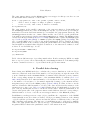
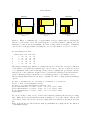
Figure 1: Effect of balancing type on approximate total processing time by showing the
subsets on each worker. Note, the actual sequence of execution might be different for load
balancing, because it is non-deterministic. For data cloning, relative performace of balancing
options can be well approximated by using the vector for the number of clones to be used.
R> clusterSize(n.clones)
1
2
3
4
5
workers none load size both
1
43
43
43
43
2
35
31
25
25
3
35
27
25
25
4
25
26
25
25
5
25
25
25
25
The function returns approximate processing times (based on the size vector) as a function
of the number of workers and balancing type. As we can see, only two workers are needed
to accomplish the task by size balancing. "none" refers to splitting the problem into subsets
without load or size balancing, "both" refers to load and size balancing, but it is identical to
"size" balancing as improvement due to load balancing cannot be determined a priori.
The plotClusterSize function can help to visualize the effect of using different balancing
options:
R>
R>
R>
R>
R>
R>
R>
opar <- par(mfrow=c(1,3), cex.lab=1.5, cex.main=1.5,
col <- heat.colors(length(n.clones))
xlim <- c(0, max(clusterSize(n.clones)[2,-1]))
plotClusterSize(2, n.clones, "none", col = col, xlim
plotClusterSize(2, n.clones, "load", col = col, xlim
plotClusterSize(2, n.clones, "size", col = col, xlim
par(opar)
cex.sub=1.5)
= xlim)
= xlim)
= xlim)
We can see in Fig. 1, that, for two workers, size balancing results in the shortest processing
time. While the model with max(n.clones) is running on one worker, all the other models
can be fitted on the other worker. Total processing time is determined by the largest problem
size.
First, we fit the five models iteratively without parallelization by using the dc.fit function
of the dclone package:
10
Parallel computing with MCMC and data cloning
R> t0 <- proc.time()
R> res3 <- dc.fit(dat, params, model, inits,
+
n.clones = n.clones, multiply = "N",
+
n.adapt = n.adapt, n.update = n.update,
+
n.iter = n.iter, thin = thin, n.chains = n.chains)
R> attr(res3, "timer") <- (proc.time() - t0)[3] / 60
Now let us fit the same models with parallelization using “socket” cluster type with two
workers. The default balancing option in dc.parfit is size balancing. The function collects
only descriptive statistics of the MCMC objects when number of clones is smaller than the
maximum, similarly to dc.fit. The whole MCMC object is returned for the MCMC object
with the largest number of clones. This approach reduces communication overhead.
R>
R>
R>
+
+
+
R>
R>
cl <- makeCluster(2, type = "SOCK")
t0 <- proc.time()
res4 <- dc.parfit(cl, dat, params, model, inits,
n.clones = n.clones, multiply = "N",
n.adapt = n.adapt, n.update = n.update,
n.iter = n.iter, thin = thin, n.chains = n.chains)
attr(res4, "timer") <- (proc.time() - t0)[3] / 60
stopCluster(cl)
Note, that by using the parallel partitioning approach to data cloning, it is not possible to
use the posterior distribution as a prior in the next iteration with higher number of clones. It
is only possible to use the same initial values for all runs, as opposed to the sequential dc.fit
function (see Sólymos (2010) and help("dc.fit") for a description of the arguments update,
updatefun, and initsfun). But opposed to the jags.parfit function which can work only
with JAGS, the dc.parfit function can work with WinBUGS and OpenBUGS as well besides
JAGS (see documentation for arguments flavour and program and examples on help pages
help("dc.parfit") and help("dc.fit")).
It took 5.74 minutes without parallelization, as compared to 3.3 minutes (57.54 %) with
parallelization. The parallel processing time in this case was close to the time needed to fit
the model with max(n.clones) = 25 clones without parallelization, so it was really the larges
problem that determined the processing time.
5. Conclusions
The paper described the parallel computing features provided by the dclone R package for
Bayesian MCMC computations and the use of the data cloning algorithm.
Large amount of parallelism can be achieved by many ways, e.g. parallelizing single chain
(Wilkinson 2005) and via graphical processing units (Suchard and Rambaut 2009; Lee et al.
2010). The parellel chains approach can be highly effective for Markov chains with good
mixing and reasonably low burn-in times. The jags.parfit function fits models with parallel
chains on separate workers by safely initializing the models, including RNG setup. Parallel
MCMC chain computations are currently implemented to work with JAGS.
Size balancing is introduced as a simple workload optimization algorithm applicable when
processing time for the pieces differ significantly. The package contains utility functions that
enable size balancing and help optimizing the workload. The dc.parfit function uses size
Péter Sólymos
11
balancing to iteratively fit models on multiple workers for data cloning. dc.parfit can work
with JAGS, WinBUGS or OpenBUGS.
The functions presented here can facilitate the analysis of larger data and complex hierarchical
models building upon commonly available Bayesian software.
6. Acknowledgments
I am grateful to Subhash Lele and Khurram Nadeem for valuable discussions. Comments
from Christian Robert and the Associate Editor greatly improved the manuscript.
References
Crowder M (1978). “Beta-Binomial ANOVA for proportions.” Applied Statistics, 27, 34–37.
Girgis IG, Schaible T, Nandy P, De Ridder F, Mathers J, Mohanty S (2007). Parallel Bayesian
methodology for population analysis. URL http://www.page-meeting.org/?abstract=
1105.
L’Ecuyer P, Simard R, Chen EJ, Kelton WD (2002). “An Object-Oriented Random-Number
Package With Many Long Streams and Substreams.” Operations Research, 50(6), 1073–
1075.
Lee A, Yau C, Giles M, Doucet A, Holmes C (2010). “On the utility of graphics cards
to perform massively parallel simulation of advanced Monte Carlo methods.” Journal of
Computational and Graphical Statistics, 19(4), 769–789.
Lele SR, Dennis B, Lutscher F (2007). “Data cloning: easy maximum likelihood estimation
for complex ecological models using Bayesian Markov chain Monte Carlo methods.” Ecology
Letters, 10, 551–563.
Lele SR, Nadeem K, Schmuland B (2010). “Estimability and likelihood inference for generalized linear mixed models using data cloning.” Journal of the American Statistical Association, 105, 1617–1625. In press.
Li N (2010). rsprng: R interface to SPRNG (Scalable Parallel Random Number Generators).
R package version 1.0, URL http://CRAN.R-project.org/package=rsprng.
Lunn D, Spiegelhalter D, Thomas A, Best N (2009). “The BUGS project: Evolution, critique
and future directions.” Statistics in Medicine, 28, 3049–3067. With discussion.
Metrum Institute (2010). bugsParallel: R scripts for parallel computation of multiple MCMC
chains with WinBUGS. URL http://code.google.com/p/bugsparallel/.
Plummer M (2010). JAGS Version 2.2.0 manual (November 7, 2010).
//mcmc-jags.sourceforge.net.
URL http:
Ponciano JM, Taper ML, Dennis B, Lele SR (2009). “Hierarchical models in ecology: confidence intervals, hypothesis testing, and model selection using data cloning.” Ecology, 90,
356–362.
12
Parallel computing with MCMC and data cloning
R Development Core Team (2010). R: A Language and Environment for Statistical Computing. R Foundation for Statistical Computing, Vienna, Austria. ISBN 3-900051-07-0, URL
http://www.R-project.org/.
Rossini A, Tierney L, Li N (2003). “Simple Parallel Statistical Computing in R.” UW Biostatistics Working Paper Series, Working Paper 193., 1–27. URL http://www.bepress.
com/uwbiostat/paper193.
Schmidberger M, Morgan M, Eddelbuettel D, Yu H, Tierney L, Mansmann U (2009). “State
of the Art in Parallel Computing with R.” Journal of Statistical Software, 31(1), 1–27.
ISSN 1548-7660. URL http://www.jstatsoft.org/v31/i01.
Sevcikova H, Rossini T (2009). rlecuyer: R interface to RNG with multiple streams. R package
version 0.3-1, URL http://CRAN.R-project.org/package=rlecuyer.
Sólymos P (2010). “dclone: Data Cloning in R.” The R Journal, 2(2), 29–37. R package
version: 1.3-1, URL http://journal.r-project.org/.
Spiegelhalter D, Thomas A, Best N, Lunn D (2007). OpenBUGS User Manual, Version 3.0.2,
September 2007. URL http://mathstat.helsinki.fi/openbugs/.
Spiegelhalter DJ, Thomas A, Best NG, Lunn D (2003). “WinBUGS Version 1.4 Users Manual.”
MRC Biostatistics Unit, Cambridge. URL http://www.mrc-bsu.cam.ac.uk/bugs/.
Suchard MA, Rambaut A (2009). “Many-Core Algorithms for Statistical Phylogenetics.”
Bioinformatics, 25(11), 1370–1376.
Tierney L, Rossini AJ, Li N, Sevcikova H (2010). snow: Simple Network of Workstations. R
package version 0.3-3, URL http://cran.r-project.org/packages=snow.
Wilkinson DJ (2005). “Parallel Bayesian Computation.” In EJ Kontoghiorghes (ed.), Handbook
of Parallel Computing and Statistics, pp. 481–512. Marcel Dekker/CRC Press.
Affiliation:
Péter Sólymos
Alberta Biodiversity Monitoring Institute
and Boreal Avian Modelling Project
Department of Biological Sciences
CW 405, Biological Sciences Bldg
University of Alberta
Edmonton, Alberta, T6G 2E9, Canada
E-mail: [email protected]