Download Biopac Student Lab Tutorial

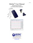
BASIC TUTORIAL
Manual Revision 3.7.3
090208
Jocelyn Mariah Kremer
Documentation
BIOPAC Systems, Inc.
William McMullen
Vice President
BIOPAC Systems, Inc.
BIOPAC® Systems, Inc.
42 Aero Camino, Goleta, CA 93117
Phone (805) 685-0066
Fax (805) 685-0067
[email protected]
www.biopac.com
Welcome to the Biopac Student Lab!
Biopac Student Lab System
The Body Electric
Waveform Concepts
Sample Data File
BSL Display
Display Tools
Scale & Grid Controls
Measurements
Markers
Menu Options
Journal
Save Data
Printing
Quit BSL
Running a Lesson
Lesson Specific Buttons
2
2
3
4
5
7
8
14
15
22
24
27
30
31
33
34
40
2
Biopac Student Lab
Welcome to the Biopac Student Lab!
This short Tutorial covers basic concepts that make the Biopac Student Lab System unique and powerful, and
provides detailed instructions on how to use important features of the program for data recording and analysis.
You are encouraged to open the Sample Data File and follow along as you complete the Tutorial. Have fun
experimenting with the display and analysis functions of the Biopac Student Lab—interacting with the software as
the Tutorial explains functionality will ease the learning curve. For more information, see your instructor or review
the Software Guide.
Biopac Student Lab System
The Biopac Student Lab System is an integrated set of software and hardware for life science data acquisition
and analysis.
Biopac Student Lab Software
Biopac Student Lab Hardware
MP3X Acquisition Unit
Transducers
Software
The inputs on the MP acquisition unit
are referred to as Channels. The
channel input ports are on the front of
the MP3X unit and are labeled CH1,
CH2, CH3, and CH4.
Th Analog Out port on the back of the
MP3X Unit allows signals to be
amplified and sent out to devices such
as headphones; on the MP36, Analog
Out is a built-in low voltage stimulator.
The Biopac Student Lab software includes 18 guided Lessons and BSL PRO options for advanced
analysis. The software will guide you through each Lesson with buttons and text and will also help you
manage data saving and data review.
Hardware Includes the MP3X Acquisition Unit (MP36, MP35 or MP30), electrodes, electrode lead cables,
transducers, headphones, connection cables, wall transformer, and other accessories.
HOW THE BIOPAC STUDENT LAB WORKS
One way to think about how the Biopac Student Lab works is to think about it as being like a video camera
connected through a VCR into a television set. In a general sense, a video camera records information about the
outside world and then converts the images it collects into an electronic format that can be passed to the VCR and
television. The images the VCR captures are stored on videotape to be archived or viewed at a later date.
Like a video camera, the Biopac Student Lab records information about the outside world, although the types of
information it collects are different. Whereas cameras record visual information, the Biopac Student Lab records
information (“signals”) about your physiological state, whether in the form of your skin temperature, the signal
from your beating heart or the flexing of an arm muscle.
Basic Tutorial
3
This physiological information is transferred via a cable from you (or whomever the information is being recorded
from) to the Biopac Student Lab. The type of physiological signals you are measuring will determine the type of
device on the end of the cable.
When the signal reaches the Biopac Student Lab, it is converted into a format that allows the data to be read by a
computer. Once that is done, the signal can be displayed on the computer screen, much like the video images from
the camera are displayed on the television set.
It takes about 1/1,000 of a second from the time a signal is picked-up by a sensor until it appears on the computer
screen. The computer’s internal memory can save these signals much like the VCR can save the video images.
Like a videotaped record, you can use the Biopac Student Lab to recall data that was collected some time ago. And
like a video, you can edit and manipulate the information stored in a Biopac Student Lab computer file.
The Biopac Student Lab software takes the signal from the MP unit and plots it as a waveform on the computer
screen. The waveform of the signal may be a direct reflection of the electrical signal from the MP channel
(amplitude is in Volts) or a different waveform that is based on the signal coming into the MP unit.
•
For example, the electrical signal into the MP unit may be an ECG signal, but the software may convert this to
display a Beats Per Minute (BPM) waveform.
The Body Electric
When most people think of electricity flowing through bodies, they think of rather unique animals, such as electric
eels, or of rare events such as being struck by lightning. What most people don’t realize is that electricity is part of
everything our bodies do...from thinking to doing aerobics—even sleeping.
In fact, physiology and electricity share a common history, with some of the
pioneering work in each field being done in the late 1700’s by Count
Alessandro Giuseppe Antonio Anastasio Volta and Luigi Galvani. Count
Volta, among other things, invented the battery and had a unit of electrical
measurement named in his honor (the Volt). These early researchers studied
“animal electricity” and were among the first to realize that applying an
electrical signal to an isolated animal muscle caused it to twitch. Even today,
many classrooms use procedures similar to Count Volta’s to demonstrate
how muscles can be electrically stimulated.
Through your lab work, you will likely see how your body generates
electricity while doing specific things like flexing a muscle or how a beating
heart produces a recognizable electric “signature.” Many of the lessons
covered in this manual measure electrical signals originating in the body. In
order to fully understand what an electrical signal is requires a basic
understanding of the physics of electricity, which properly establishes the
concept of voltages, and is too much material to present here. All you really
need to know is that electricity is always flowing in your body, and it flows
from parts of your body that are negatively charged to parts of your body that
are positively charged.
As this electricity is flowing, sensors can “tap in” to this electrical activity
and monitor it. The volt is a unit of measure of the electrical activity at any
instant of time. When we talk about an electrical signal (or just signal) we are
talking about how the voltage changes over time.
Electricity is part of everything
your body does...from thinking to
doing aerobics—even sleeping
The body’s electrical signals are detected with transducers and electrodes and sent to the MP3X acquisition unit
computer via a cable. The electrical signals can be very minute—with amplitudes sometimes in the microVolt
(1/1,000,000 of a volt) range—so the MP3X amplifies these signals, filters out unwanted electrical noise or
interfering signals, and converts these signals to a set of numbers that the computer can read. These numbers are
sent to the computer via a cable and the Biopac Student Lab software then plots these numbers as waveforms on
the computer monitor.
4
Biopac Student Lab
Waveform Concepts
A basic understanding of what the waveforms on the screen represent will be useful as you complete the lessons.
Amplitude is determined by the BSL System based on the type of MP input. The units are shown in the vertical
scale region; the unit for this example is Volts.
Time is the time from the start of the recording, which is to say that when the recording begins it does so at what
the software considers time 0. The units of time are shown in the horizontal scale region along the bottom of the
display; the unit for this example is milliseconds (1/1,000 of a second).
Units
Vertical (amplitude) Scale
start of recording
(time 0)
Units
Horizontal (time) Scale
Diving a little deeper into what a waveform represents, you are actually looking at data points that have been
connected together by straight lines.
These data points are established by the Biopac Student Lab hardware by sampling the signal inputs at consistent
time intervals. These data points can also be referred to as points, samples, or data.
The time interval is established by the sample rate of the BSL hardware, which is the number of data points the
hardware will collect in a unit of time (normally seconds or minutes). The BSL software stores these amplitude
values as a string of numbers. Since the sample rate of the data is also stored, the software can reconstruct the
waveform.
•
Sampling the data is very similar to how a VCR records images from a camera by taking snapshots of the
image at specific time intervals. When it plays back the tape, it displays the captured images in quick
succession, and our eyes can’t see the starting and stopping. Likewise, when you look at the waveform, you
see a continuous flow rather than the data points and straight lines.
The Biopac Student Lab Lessons software always uses the same sample rate for all channels on the screen, so the
horizontal time scale shown applies to all channels, but each channel has its own vertical scale. A channel’s
vertical scale units can be in Volts, milliVolts, degrees F, beats per minute, etc. A baseline is a reference point for
the height or depth (“amplitude”) of a waveform.
•
Amplitude values above the baseline
appear as a “hill” or “peak” and are
considered positive (+).
•
Amplitude values below the baseline
appear as a “trough” or “valley” and
are considered negative (−)
Basic Tutorial
5
Sample Data File
This Tutorial is designed for you to follow along with a sample data file on a computer without Biopac Student
Lab hardware attached. This means that you can complete the Tutorial on a computer outside of the
classroom/lab—perhaps at the library, computer lab or home—just as you will always have those options for
analyzing data outside the lab. Open the SampleData-L02 file as directed below.
1. Turn the computer ON.
2. Use the desktop icon or the
Windows Start menu to
open BSL Lessons 3.7.
To launch the program use desktop icon
or use the Windows® Start menu, click Programs and then select:
3. In the No Hardware mode,
the BSL software will open
to a standard Open Dialog.
Note: A hardware dialog
may be generated.
•
If the program was installed with the hardware option but there is no
hardware connected, the following dialog may be generated:
For this tutorial (and all
future analysis), click
OK to enter the Review
Saved Data mode.
4. Open the Data Files folder.
•
The program may open
the Data Files for you.
If so, skip to the next
step.
•
For future analysis, use
this dialog to browse to
your data files.
Open the Data Files folder, which is in the Biopac Student Lab
program folder.
6
Biopac Student Lab
5. Open the Sample Data
folder.
Open the Sample Data folder, which is in the Data Files folder.
6. Open the SampleData-L02
file.
Select and open the SampleData-L02 file, which is in the Sample Data
folder.
Don’t worry — you can’t lose or damage the SampleData-L02 file.
Basic Tutorial
7
BSL Display
The display includes a Data window and a Journal and both are saved together in one file.
•
The Data window displays the waveforms and is where you will perform your measurements and
analysis.
•
The Journal is where you will make notes. You can extract information from the Data window and
put it in the Journal and you can export the Journal to other programs for further analysis.
The Biopac Student Lab software has a variety of Display Tools available that allow you to change the data display
by adjusting axis scales, hiding channels, zooming in, adding grids, etc. This can be very useful when you are
interested in studying just a portion of a record, or to help you identify and isolate significant data in the record for
reporting and/or analysis.
7. Review the display to
identify the display
elements of the Data
Window and the Journal.
•
The Data Window
displays waveform(s)
during and after
recording, and is also
called the "Graph
Window." Up to eight
waveforms can be
simultaneously
displayed, as controlled
by the software and
lesson requirements.
•
The Journal works
like a standard word
processor to store
recording notes and
measurements, which
can then be copied to
another document,
saved or printed.
The SampleData-L02 file should open as shown below:
Biopac Student Lab Display
Top down, the sections of the display are:
ƒ
ƒ
ƒ
ƒ
ƒ
ƒ
ƒ
ƒ
ƒ
ƒ
ƒ
Title Bar (BSL program name and file name)
Menu Bar (File, Edit, Display, Lessons)
Tool Bar (lesson specific buttons, such as Overlap and Split)
Measurement Region (channel, type, result)
Channel Box(es) and Channel Label(s)
Marker Region (icons, text and menu)
Data window — waveform display
Horizontal scroll for Data Window
Display Tools (to the right of the Horizontal Scale) — Selection,
I-beam, and Zoom icons
Journal Tool Bar (Time and Date icons)
Journal
8
Biopac Student Lab
Display Tools
The BSL allows you complete flexibility in how the data is viewed. Chart recorders lock you into one view, but
with the BSL you can expand or compress the visual scales to aid in data analysis. The Data window display is
completely adjustable, which makes data viewing and analysis easier.
•
View multiple channels or hide channel(s) from the display view.
•
Zoom in on specific segments to take measurements, examine anomalies, etc.
•
View the entire record at one time to look for trends, locate anomalies, etc.
Editing and Selection Tools
8. Locate the editing and
selection tool icons in the
lower right of the Data
Window.
A good starting point is to understand the editing and selection tools. In the
lower right of the data window there are three icons representing the
Arrow, “I-Beam,” and Zoom tools.
To select any of these tools simply click the mouse on the desired icon, and
it will appear recessed to indicate it is active (the Selection tool is
active/recessed in the picture above).
Each tool activates a different cursor in the display window:
Arrow cursor
I-beam cursor
Channel boxes are in the upper left of the
data window. They enable you to identify
the active channel and hide channels from
view, so as to concentrate on or print out
only specific waveforms at a time.
Active Channel
9.
Click in the CH 1 box to make
that the “active channel.”
•
•
Zoom cursor
The channel box of the
active channel will be
generated to be
recessed, and the label
for the active channel
will be highlighted on
the left edge of the
channel display.
The display can Show one or more data
channels, but only one channel can be
“active” at any time. The “active” channel
box appears recessed.
The Label for the active channel is
displayed to the right of the channel boxes
and highlighted in the display region.
You can also click on
the channel label to
make a channel active.
10. Click in the CH 40 box and
note how the label changes.
CH 1 active, CH 3 and CH 40 shown
(note “Force” is highlighted on the left
edge)
CH 1 and CH 3
shown, CH 40 active
Show/Hide a channel
11. To Show or Hide a channel
hold the “Ctrl” (Control) key
down and click on the Channel
box.
a. Hide CH 40.
When you Hide a channel, the data is not lost, but simply hidden, so that
you can focus on specific channel(s). Hidden channels can be brought back
into view at any time. The channel box displays “slash marks” when it is
hidden.
Basic Tutorial
9
b. Show CH 40.
c. Hide CH 40.
•
Showing a channel
enables the channel
display but does not
make it the active
channel.
•
Hiding an active channel
does not prevent it from
being the active channel.
Show/Hide Grid Display
12. Pull down the File menu and
scroll down to select Display
Preferences.
13. Select Hide Grids to turn the
grid display OFF, and click
OK.
14. Review the display without
grids.
Another powerful feature is the ability to Show or Hide the grid display. A
grid is a series of horizontal and vertical lines that assist the eye with
finding data positions with respect to the horizontal and vertical scales. The
horizontal grid is the same for all channels (since they share the Time base),
but the vertical grid can be set for each channel.
To turn grids on and off in the Review Saved Data mode, simply choose
Display Preferences from the File menu. A Grids dialog will be generated.
Make your selection and click OK.
10
Biopac Student Lab
Note that the Grids display affects all channels. If you show a channel that
was hidden when Grids were activated, the grid display will show on the
channel.
15. Show Grids.
To adjust the grids, see Scales & Grids on page 14.
Scroll - Horizontal
16. Locate the Horizontal Scroll
Bar at the lower edge of the
display.
You can move to different locations in the record by using the horizontal
scroll bar. Since the horizontal scale applies to all channels in view, it will
move every waveform simultaneously.
The scroll bar is active when only a portion of the waveform is in view. To
move forward or backward, select and drag the scroll box or click on the
left or right arrow. For a continuous scroll, click on the arrow and hold
down the left mouse button.
If the entire waveform is displayed, the scroll bar will dim.
17. Use the Horizontal Scroll
to reposition the data with
respect to time.
•
Note that both
waveforms moved. This
is because the horizontal
scale is the same for all
channels.
In the sample file, the horizontal scale represents Time in seconds. The
software will set the most appropriate Time option for each signal.
Notice the Horizontal Scale range on the bottom changes to indicate your
position in the record.
Scroll – Vertical
18. Locate the Vertical Scroll
Bar along the right edge of
the display.
Basic Tutorial
11
A similar scroll bar can be found next to the
vertical scale. This is the Vertical Scroll Bar,
and it allows you to reposition the waveform in
the active channel. The Vertical Scroll Bar runs
along the entire right edge of the display window,
but only applies to the active channel, which is
only a portion of the display if more than one
channel is displayed.
The Vertical Scale Range for the active channel
changes when you reposition a waveform to
reflect the displayed range.
19. Use the Vertical Scroll to
reposition the CH 1 Force
waveform.
•
Note that the CH 40
Integrated EMG
waveform did not move.
This is because the
vertical scale is
independent for each
channel.
20. Pull down the Display menu
and select Autoscale
horizontal to fit the entire
waveform within the data
window.
Autoscale horizontal from the Display menu is a quick way to fit the entire
waveform within the data window. That is, it will adjust the horizontal scale
such that the left most portion of the screen is the start of the recording, and
the right most portion is the end of the recording. The time per division
setting will not necessarily be even numbers, but you can adjust that.
21. Pull down the Display menu
and select Autoscale
Waveforms to center
waveforms in their display
track.
TIP — Selecting Autoscale
Horizontal and then Autoscale
Waveforms from the Display
menu is the standard way to
quickly and easily return to your
original data display and view
12
the entire record at once.
Biopac Student Lab
The Autoscale Waveforms option of the Display menu is a very handy tool
that performs a “best fit” to each channel’s vertical scale. That is, it will
adjust the “Scale” and “Midpoint” of each channel’s vertical scale, such that
the waveform fills approximately two-thirds of the available area.
After autoscaling, the “Scale” will probably not be set to nice even numbers,
but you can manually adjust the scale to even numbers.
Zoom
22. Click on the Zoom
to select it.
icon
The Zoom
icon is in the lower right of the data window. The Zoom
function is very useful for expanding a waveform in order to see more
detail.
23. Position the cursor in the CH If you know the precise section of the waveform that you’d like to enlarge,
40 Integrated EMG channel at you can use the Zoom tool to draw a box around the area.
about 6 seconds, then click
and hold the mouse button
down and drag the cursor to
about 9 seconds. This will
draw a box around the area.
24. Release the mouse button and When the mouse button is released, the boundaries of the selected area
become the new boundaries of the data window.
review the result.
•
Note that the Horizontal
and Vertical Scales
changed for the selected
channel.
Basic Tutorial
13
The Vertical Scale will change for the active channel only, but the
Horizontal Scale will change for all channels since it (time) is the same for
all channels.
25. Select Zoom previous to
“undo” the Zoom.
After you have zoomed in on a section of the waveform, you may “undo”
the zoom and revert to the scale settings (both horizontal and vertical)
established prior to the last zoom by selecting Zoom previous from the
Display menu.
The Zoom previous function will only go back one Zoom function. You
cannot select it 6 times, for instance, to go back 6 zooms.
14
Biopac Student Lab
Scale & Grid Controls
Adjust Scales
26. Click anywhere in the
Horizontal Scale region to
generate the adjustment
dialog.
•
Review the Scale Range
and Grid settings.
If you click anywhere within the Scale region (Horizontal or Vertical) an
adjustment dialog will be generated. Any change you make to the
Horizontal or Vertical Scale only effects how the display and never alters
the saved data file. That is to say, you will never lose any data when you
change these settings.
The Vertical Scale is independent for each channel, so you need to select
the appropriate channel prior to clicking on the Vertical Scale.
27. Click anywhere in the
Vertical Scale region to
generate the adjustment
dialog.
Note that the Vertical Scale is
independent for each
channel.
•
Review the Scale Range
and Grid settings.
Scale Range: Establishes the boundary values to fit in the display window
and is useful for highlighting meaningful segments in the waveform. For
instance:
• If the signal has a cycle that repeats every 2 seconds, you could set the
Horizontal Scale Range to at 0-8 seconds to show 4 cycles per screen.
• If the signal varies from -2 to +2 Volts, you could set the Vertical
Scale Range to match and optimize the display.
Grid: The Major Division is the interval for the grid line (i.e., a horizontal
line every 2 seconds or a vertical line every 5 Kg). The Base Point is the
origin for the grid lines, with the Major Divisions drawn above and below
(horiz) or left and right (vert) to complete the grid. Minor Divisions are
also drawn in relation to the Base Point, if the lesson is set to show them.
All Channels is a quick way to have the scale setting apply to all of the
vertical scales in the data window. This is particularly useful when all of
the channels are the same type of data (i.e. 2 or 3 channels of ECG data).
Repeated clicking in the box will toggle the option on or off.
Precision: Establishes the number of significant digits displayed in the
Scale region. Click and hold down the mouse on the precision number to
generate a pop-up menu, allowing you to make another selection.
OK: Click on “OK” to initiate the changes made in the dialog.
Cancel: Click on “Cancel” to if no changes are desired.
Basic Tutorial
15
Measurements
Measurements are fast, accurate, and automatically updated. The measurement tools are used to extract
specific information from the waveform(s). Measurements are used in the Data Analysis section of every lesson,
so understanding their basic operation is important.
Let’s say you wanted to know the force increase between two clenches in the EMG data. You could get a rough
estimate by eyeballing the amplitude of the peaks on the vertical scale or by measuring the peak of one and the
peak of the next and manually calculating the difference. Or, you could take a much easier and more accurate
reading with the “delta” measurement of the Biopac Student Lab. You can use software shortcuts to paste
measurement data to the journal or copy waveform data for further analysis in other programs such as Excel.
Measurement tools
28. Review a measurement
region to identify the
Channel select box, the
Measurement type box, and
the Result box.
Measurement Region
Channel select, Measurement type, Result
The Channel select box includes
options for all channels, whether
shown or hidden, and an “SC”
measurement option. The “SC”
performs the measurement on the
active channel and is a quick way to
step through multiple channels. The
“SC” option allows you to make
quick measurement comparisons
between channels using one region.
To take a measurement from another
channel, simply click on the desired
channel box or click anywhere
within the data region for the desired
channel using the selection tool.
Channel select options
The measurement type box is a
pop-up menu next to each channel
number box that allows you to
choose from 23 Biopac Student Lab
measurement functions (or “none”).
The measurement result is the
value that the measurement
calculates.
Measurement type
options
16
Biopac Student Lab
29. Read about Measurement
Tools to the right.
To use the measurement tools, you must
a) Set the channel measurement box to the desired channel.
b) Select a measurement type from the pop-up menu.
c) Select an area for measurement.
Note that you can perform these elements in any order, but all three must be
completed to achieve a valid measurement.
Two important points regarding measurements:
1. The first is that the measurement only applies to data in the selected area of the
waveform that the user specifies.
2. The second is that every lesson contains the same measurement options, but
some may not be applicable to that particular lesson. This is because the
measurement options are a standard set of tools that are always available,
much like a scientific calculator contains a standard set of buttons, many of
which may not be necessary for any given problem.
The “selected area” for all measurements is the area selected by the I-Beam tool
(including the endpoints). Note that the “I-beam” cursor position when the mouse
30. Read about the Selected Area
button was first pressed defines the starting point and the position at release
to the right.
defines the end position of the selected area.
The Selected Area
A critical concept for the measurement tools is that the measurement results only
apply to the area established by the “I-Beam” cursor.
• The selected area can be a single point, an area, or the end points of a
selected area.
• If there is no point or area highlighted on the screen, then the
measurement results are meaningless.
• A result of **** means the selected area is not appropriate or sufficient for
the measurement.
• It is up to you to select a point or an area with the I-Beam cursor, as the
software will never do it automatically.
Select a single-point area
31. Click on the I-beam
icon.
32. Move the cursor over a point
on the data.
You will notice that whenever the cursor is over data it is displayed as an
“I.”
33. Click on the mouse button.
When you have a flashing line, you have one point of data selected. If the
line is not flashing, it means that you moved the cursor while the mouse
button was pressed, and you actually selected more than one point of data. If
this occurred simply click on another portion of data.
A flashing line should appear at
the cursor position.
34. Click on the selection tool
icon to deactivate the point.
When you are finished taking measurements, and wish to deactivate a point,
click on the selection tool icon.
Basic Tutorial
17
Selecting an area (several points)
35. Click on the I-Beam
icon.
36. Move the cursor over a point
on the data.
37. Hold the let mouse button
down and drag the mouse to
the right.
38. Release the mouse button.
•
An area should be
highlighted.
When the mouse button is released, an area should be highlighted (darkened)
on the screen, as shown above. This is very similar to how you select words
in a word processing program.
39. Click the mouse on another
When you are finished taking measurements and wish to deactivate a
point of data and then click on selected area, click the mouse on another portion of data to select just one
the selection tool icon to
point (flashing line appears), and then click on the selection tool icon.
deactivate the point.
40. Set a region for CH 1 Force
and delta.
41. Click on the I-beam
icon.
Click on the I-beam
icon to activate the I-beam cursor.
42. In the Force channel, use
the I-beam to select an area
from the peak of one clench
to the peak of the next
clench.
43. Review the result.
•
This example shows an
increase of 5.89 Kg.
Your result will vary.
If the correct region is not established by the “I-Beam” cursor for the
measurement type, the result will be meaningless.
Results will update automatically when you change the channel selection or
the selected area.
44. You can use the Data
Window options in the
Display menu to copy
measurements to another
program.
18
Biopac Student Lab
Copy Measurement — Use to copy the measurement values from the data
window to another program, such as a Word document or email for your Lab
Report.
delta(1) = 0.01392 Kg P-P(3) = 2.48267 mV
Mean(40) = 0.15282 mV
Value(1) = 0.06469 Kg
deltaT(40) = 4.19600 sec
Copy Wave Data — Use when you want to copy waveform data as a set of
numbers. The data copied will include all wave data within the area selected
by the I-beam cursor for all channels, whether displayed or hidden.
sec
4.526
4.528
4.53
4.532
4.534
Force
0.0507694
0.0507694
0.0507694
0.0507694
0.0507694
EMG
-0.0258789
-0.0224609
-0.0141602
-0.00268555
-0.0090332
Integrated EMG
0.0121948
0.0123364
0.0124744
0.0124585
0.0124524
Copy Graph — Use when you want to copy the waveform data as a picture
to be imported into other programs. The Data Window Copy functions will
be applied to the selected area, if any. If a single point or no area is selected,
the Data Window Copy functions will be applied to the entire data file.
45. You can use the Journal
options in the Edit menu to
copy measurements to the
BSL Journal.
See the Journal section for details.
Basic Tutorial
Measurement Tool
area
BPM
19
Definition
Area computes the total area among the waveform and the straight line that is drawn
between the endpoints. Area is expressed in terms of (amplitude units multiplied by
horizontal units).
The beats per minute (BPM) measurement uses the start and end points of the
selected area as a measurement for one beat, calculates the difference in time between
the first and last selected points, and divides this value into 60 seconds/minute to
extrapolate BPM. This is the result you would obtain if you took ((1/ΔT)*60) for a
selected area. If more than one beat is selected, it will not calculate the average
(mean) BPM in the selected area.
Note: In order to get an accurate BPM value, you must select an area with the I-Beam
cursor that represents one complete beat-to-beat interval. One way to do this is to
select an area that goes from the peak of one cycle’s R wave to the peak of the next
cycle’s R wave (R-R interval).
calculate
Calculate can be used to perform a calculation using the other measurement results.
For example, you can divide the mean pressure by the mean flow.
When Calculate is selected, the channel selection box disappears.
The result box will read “Off” until a calculation is performed, and then it will display
the result of the calculation. As you change the selected area, the calculation will
update automatically.
To perform a calculation, Ctrl-Click (or on PC, right mouse button click) on the
Calculate measurement type box to generate the “Waveform Arithmetic” dialog.
Use the pull-down menus to select Sources and Operand.
Measurements are listed by their position in the measurement display grid (i.e., the
top left measurement is Row A: Col 1). Only active, available channels appear in the
Source menu.
You cannot perform a calculation using the result of another calculation, so calculated
measurement channels are not available in the Source menu.
The Operand pull-down menu includes: Addition, Subtraction, Multiplication,
Division, Exponential.
The Constant entry box is activated when you select “Source: K, constant” and it
allows you to define the constant value to be used in the calculation.
20
Measurement Tool
Biopac Student Lab
Definition
To add units to the calculation result, select the Units entry box and define the unit’s
abbreviation.
Click OK to see the calculation result in the calculation measurement box
correlate
Correlate provides the Pearson product moment correlation coefficient, r, over the
selected area and reflects the extent of a linear relationship between two data sets: xi
- values of horizontal axis and f ( xi ) - values of a curve (vertical axis).
You can use Correlate to determine whether two ranges of data move together.
Association
Large values with large values
Small values with large values
Unrelated
Correlation
Positive correlation
Negative correlation
Correlation near zero
delta
The Δ (delta amplitude) measurement computes the difference in amplitude between
the last point and the first point of the selected area. It is particularly useful for taking
ECG measurements because the baseline does not have to be at zero to obtain
accurate, quick measurements.
delta S
The ΔS (delta samples) measurement is the difference in sample points between the
end and beginning of the selected area.
delta T
The ΔT (delta time) measurement is the difference in time between the end and
beginning of the selected area.
freq
The Frequency measurement converts the time segment between the endpoints of the
selected area to frequency in cycles/sec. The Freq measurement computes the
frequency in Hz between the endpoints of the selected range by computing the
reciprocal of the ΔT in that range. It will not calculate the correct frequency if the
selected area contains more than one cycle. You must carefully select the start and
end of the cycle.
Note: This measurement applies to all channels since it is calculated from the
horizontal time scale.
integral
Integral computes the integral value of the data samples between the endpoints of the
selected area. This is essentially a running summation of the data. Integral is
expressed in terms of (amplitude units multiplied by horizontal units)
This plot graphically
represents the Integral
calculation.
The area of the shaded
portion is the result.
lin_reg
Lin_reg computes the non-standard regression coefficient, which describes the unit
change in f (x) (vertical axis values) per unit change in x (horizontal axis). Linear
regression is a better method to calculate the slope when you have noisy, erratic data.
For the selected area, Lin_reg computes the linear regression of the line drawn as a
best fit for all selected data points
max
The maximum measurement finds the maximum amplitude value within the selected
area (including the endpoints).
Basic Tutorial
Measurement Tool
median
21
Definition
Median shows the median value from the selected area.
Note The median calculation is processor-intensive and can take a long time, so you
should only select “median” when you are actually ready to calculate. Until
then, set the measurement to “none.”
mean
The mean measurement computes the mean amplitude value or average of the data
samples between the endpoints of the selected area and displays the average value.
min
The minimum measurement finds the minimum amplitude value within the selected
area (including the endpoints).
none
Selecting none turns off the measurement channel and no result is provided. It’s
useful if you are copying a measurement to the clipboard or journal with a window
size such that several measurements are shown and you don’t want them all copied.
p-p
The p-p (peak-to-peak) finds the maximum value in the selected area and subtracts
the minimum value found in the selected area. P-P shows the difference between the
maximum amplitude value in the selected area and the minimum amplitude value in
the selected area.
samples
The Samples measurement shows the exact sample number of the selected waveform
at the cursor position. Since the Biopac Student Lab handles the sampling rate
automatically, this measurement is of little use for basic analysis.
slope
The slope measurement uses the endpoints of the selected area to determine the
difference in magnitude divided by the time interval. The slope measurement returns
the unstandardized regression coefficient, which describes the unit change in Y
(vertical axis values) per unit change in X (horizontal axis).
This value is normally expressed in unit change per second (rather than sample
points) since high sampling rates can artificially deflate the value of the slope. When
the horizontal axis is set to display either frequency or arbitrary units, the slope is
expressed as a unit change in vertical axis values per change in Hertz or arbitrary
units, respectively. When an area is selected, the slope measurement computes the
slope of the line drawn as a best ft for all selected data points.
stddev
Stddev (standard deviation) is a measure of the variability of data points that
computes the standard deviation value of the data samples in the selected range.
The advantage of the stddev measurement is that extreme values or artifacts do not
unduly influence the measurement.
T @ max
T @ max shows the time of the data point that represents the maximum value of the
data samples between the endpoints of the selected area.
T @ median
T @ median shows the time of the data point that represents the median value of the
selected area.
Note The median calculation is processor-intensive and can take a long time, so you
should only select “median” when you are actually ready to calculate. Until
then, set the measurement to “none.”
T @ min
T @ min shows the time of the data point that represent the minimum value of the
data samples between the endpoints of the selected area.
x-axis: T
(time)
The Time measurement shows the exact time of the selected waveform at the cursor
position. If a range of values is selected then the measurement will indicate the time
at the last position of the cursor.
value
The value measurement displays the amplitude value for the channel at the point
selected by the I-beam cursor. If a single point is selected, the value is for that point,
if an area is selected, the value is the endpoint of the selected area.
22
Biopac Student Lab
Markers
46. Read about Markers to the
right.
Markers are used to reference important locations in the data. There are two
types of markers:
Append markers – Appear as a diamond above the marker text box and
are blue when active. Append markers are automatically inserted when you
begin each new recording segment and are marked with time data
Event markers — Appear as inverted triangles below the marker text
region and are yellow when active. Event markers can be manually entered
during or after recording by pressing F9 and are pre-programmed for some
lessons.
The marker that is darkened/colored is the active marker for which the
marker text shown applies.
You may add markers to your data after it has been recorded simply by
clicking within the marker region using the selection tool. This new marker
47. Use the selection tool to click
will then become the current active marker, and you may type in the
in the marker region to the
marker text box.
right of the “Clench 3”
marker to add a new marker.
Add a marker
48. Label the new marker “test
marker” by entering text at
the flashing cursor in the
marker text region.
Select a marker
You may change the active marker
by using the “marker tools” on the
right edge of the marker region.
49. Click on the right pointing
marker tool.
Click on the right-pointing marker tool to move to the marker that was
placed after the current active marker (if one exists). Notice the marker
label and the data position.
50. Click on the left pointing
marker tool.
Click on the left-pointing marker tool to move to the marker that was
placed prior to the current active marker (if one exists). Notice the marker
label and the data position.
51. Click on the downward
pointing marker tool.
Click on the downward-pointing marker tool to generate a pop-up menu
as shown above, and drag to select an item or generate a sub-menu.
52. Pull down the downward
marker arrow and select the
Find… option.
The marker menu allows you to Find certain markers by entering the
marker text you want to locate.
53. Enter “Clench 4” when
prompted and click on Find
Next.
Basic Tutorial
23
Selecting Find again will move to the next marker with the same label (if
one exists).
54. If prompted, click OK to
restart marker search from
the beginning of the record.
55. Select the Clear option to
delete the “Test marker.”
You cannot clear Append Markers, so these options only apply to Event
Markers. Clear Active Event Marker will delete the active Event Marker
if one is selected, and Clear All Event Markers will delete all Event
Markers in the file.
You cannot undo a “Clear” function, so use caution when
selecting these functions.
56. Select the Summary to
Journal option.
These options will paste marker information to the Journal and format the
data with an Index, Time, and Label. The “All markers” option will list
markers by time, which may mix the Event Markers with Append Markers.
57. Select the Show option.
Review the list of marker
labels at the bottom of the
menu and scroll down to
select Clench 4.
Generate a list of markers. Drag to select a marker and jump to it in the
display.
All the marker labels in the record will be listed at the bottom of the menu.
The SampleData-L02 file has two markers. You may go to a particular
marker by scrolling down to select its label.
• Moving to different markers using this menu may not seem very
relevant for the SampleData-L02 file, but when a lot of data has been
recorded, it can be a very useful tool.
24
Biopac Student Lab
58. Select the Preferences
option.
Use the Journal Summary tab to set options for ordering and formatting
the Summary to Journal option.
Note: The rest of the Marker Preferences are advanced functions for
automating marker creation and labeling—your instructor will
provide details as needed when you run a Lesson.
Menu Options
59. Click on the File menu and
review the options.
Save As allows you to save to your
school’s network or other media so you
can access the file outside of the lab or
send Journal reports to your instructor.
60. Click on the Edit menu and
review the options and suboptions.
61. Click on the Display menu and
review the options.
TIP: Use Autoscale Horizontal
followed by Autoscale Waveforms to
view all the data in one screen and
restore the data display to its original
state.
Basic Tutorial
25
62. Click on the Lessons menu
and review the options.
BSL PRO Note —
If your instructor set BSL
Lesson preferences to
activate the BSL PRO
software controls in the
Review Saved Data mode,
the menus will include
selected PRO options for
advanced analysis.
See your instructor or the
BSL PRO Software Guide
for functionality details.
• Lessons menu stays the
same
• Help menu stays the
same
• Transform menu is
only available in PRO
mode
BSL AnalysisMode
BSL PRO Analysis Mode
26
Biopac Student Lab
Basic Tutorial
27
Journal
63. Read about the Journal to
the right.
The Review Saved Data mode incorporates a Journal feature so you can
type notes or copy measurements from previously saved data. You can
also copy data directly to the Journal. The Journal needs to be the active
window for its options to come up.
64. Click anywhere in the
Journal window to activate
it.
65. Click on the bar separating
the Journal window from the
Data window and drag up or
down to resize the Journal.
Format Journal Entries
66. Pull down the File menu,
scroll down to Journal
Preferences.
You can control formatting for text, measurements and wave data. Click
67. Review the options that can
on the “Change Font” button to set the text font, style and size.
be set to change the way
measurements are pasted into
the Journal.
68. Click in the box next to each
measurement paste option
box so that all are selected.
69. Click in the “Include time
values” box in the Wave Data
Paste Options section.
70. Click OK to accept the
option changes.
Select these options so that when you paste measurements you can easily
identify them.
Note When you plan to export the measurements to a spreadsheet
program (such as Excel), it is best not to select all of the
Measurements Paste Options or the Wave Data Paste Option as
these will affect the formatting.
28
Biopac Student Lab
Time and Date Stamps
71. Position the cursor at the end
of the journal entries and
click on the clock icon to
activate the time stamp.
The Journal has stamps for the time and date, which can be useful when
creating reports. The icons are on the left edge of the Journal toolbar.
The time stamp is the “clock” icon at the top left of the Journal window.
When you click on the clock icon, the current time (according to your
computer’s System clock) will be entered in the Journal at the cursor
point.
10:36:20 AM
Review the result.
72. Click on the calendar icon to
activate the date stamp.
Review the result.
Text entry
73. Place the cursor at the point
you wish to begin typing and
enter text using the standard
keyboard functions.
Paste Measurement(s) to Journal
74. Read about the Paste
Measurement function.
The date stamp is the “calendar” button to the right of the time stamp.
When you click on the calendar icon, the current date (according to your
computer’s System calendar) will be entered in the Journal at the cursor
point.
Tuesday, December 30, 2003
It’s possible to write anything you want directly in the Journal. Just click
on the Journal window and place the cursor at the point you wish to
begin typing.
When you use the Paste Measurement function, all the pop-up
measurements showing a value will be written to the Journal.
TIP Use the “none” measurement option when you don’t want a
measurement pasted to the Journal.
To paste a pop-up measurement into the Journal:
1. Select the channel you want to measure by clicking on it with the
Selection tool or use the cursor to pick the correct channel number
in the boxes just left of each of the pop-up measurements.
2. Choose the appropriate pop-up measurement.
3. Use the I-beam tool to select the portion of the wave you are
interested in.
The pop-up measurement values will update instantly. The pop-up
measurements always operate on the selected area you have chosen
with the I-beam tool.
•
4.
For instance, if you choose p-p, you will find the peak to peak
value of the wave in the selected area. If you choose max, you
will get the maximum value of the wave in the selected area.
Pull down the Edit menu and select Journal>Paste Measurement.
Alternatively, you can use the Ctrl-M keystroke command.
Basic Tutorial
75. Select Channel 1 in the Data
Window.
29
Select the channel you want to measure by clicking on it with the arrow
tool or use the cursor to pick the correct channel number in the boxes just
left of each of the pop-up measurements.
76. Set a pop-up measurement
box for CH 1 mean.
77. Set a second pop-up
measurement box for CH 40
mean.
78. Use the I-beam tool to select
a region from the peak of one
R-wave to the peak of the
next R-wave.
79. Pull down the Edit menu,
scroll to Journal and slide
right to select Paste
Measurement.
80. Review the Journal entry.
Paste Wave Data to Journal
81. Read about the Paste Wave
Data function.
The Paste Wave Data function will write all the points that make up the
data in the selected wave area to the Journal.
Note It’s very easy to put a lot of data into the Journal using this
command: One second of a wave that was sampled at 200 Hz will
paste 200 numbers into the Journal.
To paste wave data into the Journal:
a. Select the channel you wish to measure by clicking on it using the
Selection tool or use the cursor to pick the correct channel in the
channel boxes just left of each of the pop-up measurements. This
will activate the Data Window.
b. Use the I-beam tool to select the portion of the wave you are
interested in.
c. Pull down the Edit menu and scroll down to Journal then scroll right
to Paste Wave Data.
82. Use the I-beam selection tool
to select the portion of the
wave you are interested in.
83. Pull down the Edit menu,
scroll down to Journal then
scroll right to Paste Wave
Data.
84. Review the Journal entry.
85. Export Journal Files
The Journal file is saved in standard text format and can be exported to
word processing or spreadsheet programs—or any application that
accepts Text or ASCII files.
To export Journal text and/or data to another program:
a. Open the BSL file.
b. Select the desired Journal text.
c. Choose Edit>Copy to copy the Journal text.
d. Switch to the other program.
30
Biopac Student Lab
e. Choose Edit>Paste to paste the copied data.
Note When you plan to place the data into a spreadsheet, it’s usually a
good idea to remove any extraneous comments, so you just have
rows and/or columns of numbers.
Saving the Journal
86. To save with the existing file
name and location, click on
the File menu and select Save
Changes.
Use the File menu Save options to save the Journal. The Journal and
Graph files are linked and will be opened and saved together.
87. To save with a new file name
and/or location, click on the
File menu and select Save
As.
Save Data
88. Read about the Save
functions to the right.
Each student’s recording is automatically saved at the end of each
lesson recording. Students do not need to resave files unless they
significantly alter the data window settings or make a change to
the journal while in the Review Saved Data mode.
Once in the Review Saved Data mode, you may alter the data
display window, or enter more information into the journal. When
you make changes to the data window, you are only changing
how the data appears on the screen — you are not altering the
data that was originally recorded. Saving the changes will never
delete any data.
89. Review the save options
under the File menu.
•
Save Changes
•
Save As (new name or
location)
90. Pull down the File menu and
select the Save changes
option.
91. Pull down the File menu and
select the Save As option.
Save Changes
We recommend this option to ensure that lesson files are properly
named and saved.
Saves the file with the existing file name and location.
Save As
To take data home for analysis, use this option.
Creates a copy of the original file and prompts you for a location
to save the copy to — floppy, network, or other media.
The save is automatic, no dialog or confirmation is required.
The following dialog will be generated so you can designate a
location for the file.
Basic Tutorial
31
File name cannot be altered from the original name. This allows
the Review Saved Data mode to work correctly.
Save as type is locked on “Lesson Files,” which is the original
way the file was saved and is the waveform display you
normally see on screen. This mode copies the journal text as
well.
The “Save” button instigates the Save function.
Printing
92. Read about the Print
functions to the right.
TIP: It’s always a good idea to
Save before printing.
You control how the data is presented on the printed page by
controlling how it is displayed on the screen prior to selecting Print.
All of the options relating to printing the data files apply to the
waveforms as they are displayed in the data window. If you’ve
zoomed, changed the scale, or hidden a channel, only the portion of
data displayed in the data window will be printed. This is actually very
useful, because oftentimes you may only want to display a portion of
the data.
When you choose File>Print you will be prompted to choose which
items to print.
Print Graph
IMPORTANT! The printer
only works with the data shown
in the data window, which often
is not the complete data file.
The following Print dialog is just an example. Your actual Print dialog
will depend on the printer and Operating System you are using. The
dialog should include Print Options that allow you to control how
much data is printed on each page.
• Depending on your OS, you may need to access the Print
Options via a button in the original Print dialog. Refer to the
Users Manual for your computer and/or printer for more detail.
32
Biopac Student Lab
•
Print Options
Print ___ plots per page
This option determines how each page will be divided up to plot
the data displayed in the data window.
•
For example, entering “4” will divide each page into four
regions.
The printed data may have an expanded time scale if the printer
made adjustments to plot what was viewed on the screen evenly
across the specified area.
Fit to ___ pages
This option determines how many pages to use to print what is
displayed on the screen.
•
• Automatic Adjustments
For example, entering “2” will print the data displayed in the
window evenly across two pages. The first (left) part of the
data displayed on screen would print on Page 1 and the second
(right) part would print on Page 2.
The software will automatically make the following adjustments prior
to printing, which may result in slight differences between what is
displayed and what is printed:
• Vertical Scale — If a vertical scale in the data window is set
to fractional numbers, then the software will slightly adjust the
scale to use even numbers for print.
• Markers — When markers are displayed on the screen with
associated marker text, the data will print with the marker text
directly above the appropriate marker and a dashed vertical
line will run through the data to indicate the marker’s precise
point in time. If the data is compressed, the markers and/or
marker text may overlap or be hidden. If this is not acceptable,
then you’ll need to expand the time scale so that the markers
have enough room to print.
Print Journal
93. Print the entire data file
a. Click anywhere in the Data
Window to make it the active
window.
b. Choose Display>Autoscale
Horizontal.
c. Choose Display>Autoscale
Waveforms.
d. Choose File>Print>Print
Graph.
e. Set Plots per page and Fit to
pages as desired.
f. Click OK.
94. Review the printed result.
This option generates a standard Print dialog to print the Journal text.
Basic Tutorial
33
Quit BSL
95. Pull down the file menu and
select Quit.
icon in the
During the recording mode, the application close
upper right corner of the display window is blocked so you can’t
inadvertently quit the application when you simply meant to close
the data window.
To quit the application, you need to choose Quit from the File
menu.
If Quit is blocked, click on the STOP button and wait for the
recording to end, then try Quit again.
96. If prompted, click Yes to
save all changes.
97. Close the file you opened and
close the hard drive window.
When you try to quit the software after altering the data file
and/or journal file in any way, the following message will be
generated.
34
Biopac Student Lab
Running a Lesson
To run a BSL Lesson, you must have an MP3X data acquisition unit connected. If you installed the BSL software
with the Hardware option and have an MP3X unit connected, you can follow along on your computer; otherwise
just read this section so you’ll know what to expect in the lab.
IMPORTANT — You are free to download the Biopac Student Lab Analysis software for
use on your personal computer. The hardware does not have to be attached for you to
review and analyze your data files. See www.biopac.com for the BSL Analysis download.
The primary objective of the Recording section is to assist you in obtaining good data, and the primary objective of
the Analysis is to help you understand the data and the physiological concept it represents. Lessons are set up so
that you can record data in the lab and then analyze the data after class—in the lab or at home.
FAST TRACK
Detailed Explanation of Steps
This side of the lesson (left, shaded
column) is the “FAST TRACK” through
the lesson, which contains a basic
explanation of each step.
This side of the lesson contains more detailed
information to clarify the steps and/or concepts in the
FAST TRACK, and may include reference diagrams,
illustrations, screen shots, and/or references to this
manual.
Although it is not absolutely necessary, BIOPAC recommends that students work in groups of at least three.
Students should choose a Director, a Recorder, and a Subject from their lab group before beginning Set Up
(which often involves the Subject).
Director
The Director reads the lesson steps and tells the Recorder and Subject what to do. The Director also
keeps track of the length of time for each condition.
Recorder During the recording session, the Recorder will insert a marker (press F9 on PC or Esc on Mac)
whenever the Subject is requested to do something and will key in the condition to create the marker
label. The recording step will indicate what to key in. Note that marker text can be added or edited
after the recording is complete.
Subject
This is the person from whom data will be recorded. The Subject will need to perform the tasks as
instructed by the Director. It is suggested that the Subject not look at the computer screen while data
is being recorded, as there tends to be a “biofeedback” effect that can bias the heart rate.
1. Turn the computer ON.
To run a lesson, the computer must have an MP unit connected.
2. Use the desktop icon or the
Windows Start menu to open
Biopac Student Lab 3.7.
To launch the program, use the desktop icon
or the Windows® Start menu and choose Programs and then select:
Basic Tutorial
35
3. Click on the Lessons menu
and select a Lesson.
• The Review Saved Data
option will generate a
standard Open dialog so
you can select a file for
analysis.
If the hardware is not connected, the following prompt will be
generated. To run a lesson, check the power and connections for the
MP unit and then click Retry.
4. Type in your file name.
Type in your name so the BSL System can store all of your data files
in one place, and make it easier for you to retrieve data later on.
You can enter your real name, a nickname, or the name of your group
if you are working with other students. Select and type in a unique
identifier, such as the Subject’s nickname or student I.D. #, your full
name or some combination of your name and other letters and/or
numbers (like JohnF or John3). It is a good idea to use the same logon name for each lesson. Be sure to write down the log-on name you
choose so that you can keep track of where your data is stored.
The Biopac Student Lab software will let you use the same name ten
times. If there are a lot of other students using your computer and you
try to log on with a general name (“John” vs. “JohnF”) there is a good
chance the Biopac Student Lab software will ask you to use a
different name.
36
Biopac Student Lab
If you know the existing folder is your own, select Use it. This is a
convenient way to ensure that all of your lesson files for the class
term are stored in one folder. If you Rename the folder, just add a
character to the last name you used, i.e. “Lauren” becomes
“Lauren2.” Once you enter your name and choose OK, the Biopac
Student Lab software creates a folder inside the “Data Files” folder
that is inside the “Biopac Student Lab” folder on your computer (or in
an alternate location if your instructor modified setup). This is where
all your data will be stored. If you choose the same file name for other
lessons, they will also be stored in this folder (with the appropriate
lesson number extension).
If you try to use the same file name an eleventh time, the program
will insist that you choose a different name.
The files inside your folder can be moved, copied, or duplicated, just
like any other file. If you wish, you can copy them to a “floppy disk”
as a backup or to be viewed later. Check with your instructor or lab
assistant for more information on how to do this.
When you run a lesson, the first step is a prompt for you to enter your
name. The Biopac Student Lab software creates a folder with the
exact name you enter and places it in the Data Files folder of the
Biopac Student Lab Program folder. When you press the Done button
in the lesson to end recording, the BSL program automatically saves
your waveform data file to the Data Files folder with a file name
based on the user name or I.D. given at the start of each lesson.
The software will save the data file with the name you entered plus an
extension that identifies the lesson number. This extension is very
important because the software will key off this extension and open
up different tools for the Review Saved Data Mode, depending on the
lesson.
Other lesson data files that use the same name will be placed in this
same folder, but the software will never allow you to save a data file
with the same name and lesson number.
As a general note, because the Biopac Student Lab software
automatically is saving the files, you must exercise caution when
moving things around into different folders.
It is recommended that you never place other files or folders in the
Biopac Student Lab folder, and never take files or folders out of the
BSL 3.7 folder with the exception of removing data files from the
Data Files folder.
Basic Tutorial
37
5. Follow the instructions in the
lesson manual and in the
Journal, or proceed as directed
by your instructor.
The recording section is very detailed and includes sample screen
shots for comparison—so, even if you don’t fully understand what is
happening when you’re running the lesson or feel pressured by time
(as is often the case), you should be able to obtain good, meaningful
data. Then, you’ll be able to analyze and grasp the important concepts
later, during the Analysis section.
Normally, there are multiple data segments that need to be recorded,
with different tasks occurring during and/or between these segments.
It is important that you read ahead to the next step in the lesson so it
is clear what task(s) you’ll need to perform during each recording
segment.
6. Step through the lesson as
guided in the Lesson manual
or by your instructor.
To begin a Lesson, click on the Calibrate button. The dynamic
calibration procedure will automatically optimize the BSL System for
the signal(s) being recorded in the lesson.
• With equipment such as an oscilloscope, you or your instructor
needed to “twiddle” with the dials and switches, e.g., gain or
amplification settings, position (vertical or horizontal alignment),
voltage/division settings, time/division settings, and sweep speed
to make sure a “good” signal was recorded. This entire procedure
had to be manually repeated for each new subject. The Biopac
Student Lab makes the required adjustments for you during the
automatic calibration procedure.
If you did not plug in the hardware as directed, you will be prompted
to correct it before continuing.
A dialog will help you prepare for the each segment. Read the
instructions and click OK to continue.
38
Biopac Student Lab
The calibration routine will stop automatically.
If your calibration data does not match the sample screen shot
provided, click on Redo Calibration to repeat calibration and erase
the old data.
If your calibration data matches the sample screen shot, click on
Record to begin the first recording segment.
Click on “Suspend” when you have completed the assigned segment
task(s).
• You should click on “Suspend” as soon as possible once you have
completed a segment. This is important because every second
wasted is memory used up for the data recording. The more
memory used, the slower the program will operate, the more disk
space will be used up when the data is saved, and the more
possibility of problems.
• When selected, the Suspend button toggles to “Resume.”
Review Recorded Data
When you Suspend recording between lesson segments, you
can check that you have good data before continuing. You may
want to check your data by zooming in on a segment, taking a
measurement, adding grids, etc. Review your data before
continuing and read ahead to prepare for the next segment.
The Arrow, “I-Beam,” and Zoom tools are inactive (greyed) during
recording but can be used between segments while in the Recording
mode. The Display menu items are also available.
To repeat the last recorded section and erase the old data, click on
Redo.
• The “Redo” feature is very handy and should prevent you from
panicking during the recording. You can redo a recording segment
if something goes wrong or if you realize you have not performed
the proper tasks.
If you are finished with the data recordings, click on Stop.
Click the “Done” button in the Lesson display to generate the closing
options dialog.
Basic Tutorial
39
Record from another subject will return you to the first screen of
the lesson. Repeat the necessary set up, type in a new Subject name,
and repeat the entire recording. Depending on the lesson, you may or
may not have to redo the calibration.
Analyze current data file will switch you to the Review Saved Data
mode and will automatically open the last recorded data file.
Analyze another data file will switch you to the Review Saved Data
mode and will prompt you to find and open a data file for review.
Record Another Lesson will generate the lessons menu.
Copy to Floppy or Network will generate a Save dialog, allowing
you to designate the location to save the file to. Note that you cannot
change the File name.
7. Save the recorded lesson data.
Review Saved Data Mode
for Data Analysis
Quit will close all lesson windows that are open and then exit the
Biopac Student Lab program.
Each student’s recording is automatically saved at the end of each
lesson recording. You do not need to resave files unless you
significantly alter the data window settings or make a change to the
Journal while in the Review Saved Data mode. You will be prompted
to save changes.
Data Analysis is where you analyze your data to “pull out”
measurements that reinforce the concepts presented in the
Introduction. Analysis can be done right after the data is recorded, or
can be done off-line on another computer (the hardware does not need
to be attached). The analysis should be done after all students have
recorded their data.
Measurements taken in the Analysis section are to be placed in the
Data Report section and may also be placed in the on-screen journal
for saving and printing. Whenever a measurement needs to be placed
in the Data Report, a reference icon will direct you to the proper
section of the Data Report.
40
Biopac Student Lab
Lesson Specific Buttons
Some lessons have extra buttons (under the menu bar) for features appropriate to the lesson signal and/or protocol.
The following buttons are not in the sample file, so just read about them below.
The Listen button allows you to listen to the signal as output if you have
headphones or other listening hardware connected.
The Overlap and Split buttons allow you to merge or separate the data
channels (“tracks”) in the display window.
You cannot successfully apply grids after the Overlap function is
activated. Grids can change the scale, so begin in the Split mode, then
apply grids, then Autoscale, then apply the Overlap.
The Adjust Baseline button is only used in “Lesson 5 ECG I” and it
allows you to position the waveform up or down in small increments so
that the baseline can be exactly zero. This is not necessary to get
accurate amplitude measurements, but may be desired before making a
printout or when using grids.
When you click the Adjust Baseline button, Up and Down buttons will
be generated. Simply click on these to move the waveform up or down.
The Exit button will close the Adjust Baseline options and return to the
waveform display.
These buttons are in Lesson 3 and will filter the signal into the
bandwidth for alpha, beta, delta and theta analysis.
Basic Tutorial
41
Legalese
Copyright
Information in this document is subject to change without notice and does not represent a commitment on the part
of BIOPAC Systems, Inc. This tutorial and the software it describes are copyrighted with all rights reserved. Under
copyright laws, this tutorial or the software may not be copied, in whole or part, without the written consent of
BIOPAC Systems, Inc., except in the normal use of the software or to make a backup copy.
The same proprietary and copyright notices must be affixed to any permitted copies as were affixed to the original.
This exception does not allow copies to be made for others, whether or not sold, but all of the material purchased
(with all backup copies) may be sold, given, or loaned to another person. Under the law, copying includes
translating into another language or format.
Biopac Student Lab Tutorial, including all text and graphics, are ©1998-2008 BIOPAC Systems, Inc., with all
rights reserved.
Warranty
BIOPAC Systems, Inc. warrants its hardware products against defects in materials and workmanship for a period
of 12 months from the date of purchase. If BIOPAC Systems, Inc. receives notice of such defects during the
warranty period, it will, at its option, repair or replace the hardware products that prove to be defective.
This warranty applies only if your BIOPAC Systems, Inc. product fails to function properly under normal use and
within the manufacturer’s specifications. This warranty does not apply if, in the sole opinion of BIOPAC Systems,
Inc., the BIOPAC product has been damaged by accident, misuse, neglect, improper packing, shipping,
modification, or servicing by other than BIOPAC Systems, Inc.
Any returns should be supported by a Return Mail Authorization (RMA) number issued by BIOPAC Systems, Inc.
BIOPAC Systems, Inc. reserves the right to refuse delivery of any shipment containing any shipping carton
without the RMA number(s) displayed on the outside. The Buyer shall prepay transportation charges to the site
designated by BIOPAC Systems, Inc.
BIOPAC Systems, Inc. makes no warranty or representation, either expressed or implied, with respect to this
software, its quality, performance, merchantability, or fitness for a particular purpose. As a result, this software is
sold “as is” and you, the Buyer, are assuming the entire risk as to its quality and performance.
In no event will BIOPAC Systems, Inc. be liable for direct, indirect, special, incidental, or consequential damages
resulting from any defect in the software or its documentation, even if advised of the possibility of such damages,
or for damage of any equipment connected to a BIOPAC Systems, Inc. product.
Trademarks
BIOPAC is a registered trademark of BIOPAC Systems, Inc.
Apple and Macintosh are trademarks of Apple Computer, Inc.
Windows is a trademark of Microsoft Corporation.
This document was created with Microsoft Word for Windows, Adobe Photoshop, Corel Draw 7.0. Mainstay
Capture, and JASC, Inc. JasCapture.