1
Automated analysis of security protocols with global state
(Full version)
Steve Kremer
INRIA Nancy - Grand’Est & Loria, France
arXiv:1403.1142v2 [cs.CR] 12 May 2014
Robert Künnemann∗
Department of Computer Science, TU Darmstadt, Germany
Abstract
Security APIs, key servers and protocols that need to keep the status of transactions, require to
maintain a global, non-monotonic state, e.g., in the form of a database or register. However, most
existing automated verification tools do not support the analysis of such stateful security protocols
– sometimes because of fundamental reasons, such as the encoding of the protocol as Horn clauses,
which are inherently monotonic. A notable exception is the recent tamarin prover which allows
specifying protocols as multiset rewrite (msr) rules, a formalism expressive enough to encode state.
As multiset rewriting is a “low-level” specification language with no direct support for concurrent
message passing, encoding protocols correctly is a difficult and error-prone process.
We propose a process calculus which is a variant of the applied pi calculus with constructs
for manipulation of a global state by processes running in parallel. We show that this language
can be translated to msr rules whilst preserving all security properties expressible in a dedicated
first-order logic for security properties. The translation has been implemented in a prototype tool
which uses the tamarin prover as a backend. We apply the tool to several case studies among which
a simplified fragment of PKCS#11, the Yubikey security token, and an optimistic contract signing
protocol.
1
Introduction
Automated analysis of security protocols has been extremely successful. Using automated tools, flaws
have been for instance discovered in the Google Single Sign On Protocol [5], in commercial security
tokens implementing the PKCS#11 standard [10], and one may also recall Lowe’s attack [21] on the
Needham-Schroeder public key protocol 17 years after its publication. While efficient tools such as
ProVerif [7], AVISPA [4] or Maude-NPA [14] exist, these tools fail to analyze protocols that require
non-monotonic global state, i.e., some database, register or memory location that can be read and
altered by different parallel threads. In particular ProVerif, one of the most efficient and widely used
protocol analysis tools, relies on an abstraction that encodes protocols in first-order Horn clauses. This
abstraction is well suited for the monotonic knowledge of an attacker (who never forgets), makes the
tool extremely efficient for verifying an unbounded number of protocol sessions and allows to build on
existing techniques for Horn clause resolution. However, Horn clauses are inherently monotonic: once
a fact is true it cannot be set to false anymore. As a result, even though ProVerif’s input language,
a variant of the applied pi calculus [2], allows a priori encodings of a global memory, the abstractions
performed by ProVerif introduce false attacks. In the ProVerif user manual [8, Section 6.3.3] such an
encoding of memory cells and its limitations are indeed explicitly discussed: “Due to the abstractions
performed by ProVerif, such a cell is treated in an approximate way: all values written in the cell are
considered as a set, and when one reads the cell, ProVerif just guarantees that the obtained value is one
∗
Most of this work was carried out when the author was affiliated to INRIA Paris - Rocquencourt, France
1
of the written values (not necessarily the last one, and not necessarily one written before the read).”
Some work [3, 22, 12] has nevertheless used ingenious encodings of mutable state in Horn clauses, but
these encodings have limitations that we discuss below.
A prominent example where non-monotonic global state appears are security APIs, such as the
RSA PKCS#11 standard [23], IBM’s CCA [11] or the trusted platform module (TPM) [27]. They have
been known to be vulnerable to logical attacks for some time [20, 9] and formal analysis has shown
to be a valuable tool to identify attacks and find secure configurations. One promising paradigm for
analyzing security APIs is to regard them as a participant in a protocol and use existing analysis tools.
However, Herzog [18] already identified not accounting for mutable global state as a major barrier to the
application of security protocol analysis tools to verify security APIs. Apart from security APIs many
other protocols need to maintain databases: key servers need to store the status of keys, in optimistic
contract signing protocols a trusted party maintains the status of a contract, RFID protocols maintain
the status of tags and more generally websites may need to store the current status of transactions.
Our contributions We propose a tool for analyzing protocols that may involve non-monotonic
global state, relying on Schmidt et al.’s tamarin tool [25, 26] as a backend. We designed a new
process calculus that extends the applied pi calculus by defining, in addition to the usual constructs
for specifying concurrent processes, constructs for explicitly manipulating global state. This calculus
serves as the tool’s input language. The heart of our tool is a translation from this extended applied
pi calculus to a set of multiset rewrite rules that can then be analyzed by tamarin which we use
as a backend. We prove the correctness of this translation and show that it preserves all properties
expressible in a dedicated first order logic for expressing security properties. As a result, relying on the
tamarin prover, we can analyze protocols without bounding the number of sessions, nor making any
abstractions. Moreover it allows to model a wide range of cryptographic primitives by the means of
equational theories. As the underlying verification problem is undecidable, tamarin may not terminate.
However, it offers an interactive mode with a GUI which allows to manually guide the tool in its proof.
Our specification language includes support for private channels, global state and locking mechanisms
(which are crucial to write meaningful programs in which concurrent threads manipulate a common
memory). The translation has been carefully engineered in order to favor termination by tamarin. We
illustrate the tool on several case studies: a simple security API in the style of PKCS#11, a complex
case study of the Yubikey security device, as well as several examples analyzed by other tools that aim
at analyzing stateful protocols. In all of these case studies we were able to avoid restrictions that were
necessary in previous works.
Related work The most closely related work is the StatVerif tool by Arapinis et al. [3]. They
propose an extension of the applied pi calculus, similar to ours, which is translated to Horn clauses
and analyzed by the ProVerif tool. Their translation is sound but allows for false attacks, limiting
the scope of protocols that can be analyzed. Moreover, StatVerif can only handle a finite number of
memory cells: when analyzing an optimistic contract signing protocol this appeared to be a limitation
and only the status of a single contract was modeled, providing a manual proof to justify the correctness
of this abstraction. Finally, StatVerif is limited to the verification of secrecy properties. As illustrated
by the Yubikey case study, our work is more general and we are able to analyze complex injective
correspondance properties.
Mödersheim [22] proposed a language with support for sets together with an abstraction where all
objects that belong to the same sets are identified. His language, which is an extension of the low
level AVISPA intermediate format, is compiled into Horn clauses that are then analyzed, e. g., using
ProVerif. His approach is tightly linked to this particular abstraction limiting the scope of applicability.
Mödersheim also discusses the need for a more high-level specification level which we provide in this
work.
There has also been work tailored to particular applications. In [13], Delaune et al. show by a
dedicated hand proof that for analyzing PKCS#11 one may bound the message size. Their analysis
still requires to artificially bound the number of keys. Similarly in spirit, Delaune et al. [12] give a
dedicated result for analyzing protocols based on the TPM and its registers. However, the number of
2
reboots (which reinitialize registers) needs to be limited.
Guttman [17] also extended the strand space model by adding support for state. While the protocol
execution is modeled using the classical strand spaces model, state is modeled by a multiset of facts,
and manipulated by multiset rewrite rules. The extended model has been used for analyzing by hand
an optimistic contract signing protocol. As of now, protocol analysis in the strand space model with
state has not been mechanized yet.
In the goal of relating different approaches for protocol analysis Bistarelli et al. [6] also proposed
a translation from a process algebra to multiset rewriting: they do however not consider private
channels, have no support for global state and assume that processes have a particular structure.
These limitations significantly simplify the translation and its correctness proof. Moreover their work
does not include any tool support for automated verification.
Obviously any protocol that we are able to analyze can be directly analyzed by the tamarin
prover [25, 26] as the rules produced by our translation could have been given directly as an input
to tamarin. Indeed, tamarin has already been used for analyzing a model of the Yubikey device [19],
the case studies presented with Mödersheim’s abstraction, as well as those presented with StatVerif.
It is furthermore able to reproduce the aforementioned results on PKCS#11 [13] and the TPM [12] –
moreover, it does so without bounding the number of keys, security devices, reboots, etc. Contrary
to ProVerif, tamarin sometimes requires additional typing lemmas which are used to guide the proof.
These lemmas need to be written by hand (but are proved automatically). In our case studies we also
needed to provide a few such lemmas manually. In our opinion, an important disadvantage of tamarin
is that protocols are modeled as a set of multiset rewrite rules. This representations is very low level
and far away from actual protocol implementations, making it very difficult to model a protocol adequately. Encoding private channels, nested replications and locking mechanisms directly as multiset
rewrite rules is a tricky and error prone task. As a result we observed that, in practice, the protocol
models tend to be simplified. For instance, locking mechanisms are often omitted, modeling protocol
steps as a single rule and making them effectively atomic. Such more abstract models may obscure
issues in concurrent protocol steps and increase the risk of implicitly excluding attacks in the model
that are well possible in a real implementation, e. g., race conditions. Using a more high-level specification language, such as our process calculus, arguably eases protocol specification and overcomes
some of these risks.
2
Preliminaries
Terms and equational theories As usual in symbolic protocol analysis we model messages by
abstract terms. Therefore we define an order-sorted term algebra with the sort msg and two incomparable subsorts pub and fresh. For each of these subsorts we assume a countably infinite set of names,
FN for fresh names and PN for public names. Fresh names will be used to model cryptographic keys
and nonces while public names model publicly known values. We furthermore assume a countably
infinite set of variables for each sort s, Vs and let V be the union of the set of variables for all sorts.
We write u : s when the name or variable u is of sort s. Let Σ be a signature, i.e., a set of function
symbols, each with an arity. We write f /n when function symbol f is of arity n. We denote by TΣ the
set of well-sorted terms built over Σ, PN , FN and V. For a term t we denote by names(t), respectively
vars(t) the set of names, respectively variables, appearing in t. The set of ground terms, i.e., terms
without variables, is denoted by MΣ . When Σ is fixed or clear from the context we often omit it and
simply write T for TΣ and M for MΣ .
We equip the term algebra with an equational theory E, that is a finite set of equations of the form
M = N where M, N ∈ T . From the equational theory we define the binary relation =E on terms,
which is the smallest equivalence relation containing equations in E that is closed under application of
function symbols, bijective renaming of names and substitution of variables by terms of the same sort.
Furthermore, we require E to distinguish different fresh names, i. e., ∀a, b ∈ FN : a 6= b ⇒ a 6=E b.
Example. Symmetric encryption can be modelled using a signature
Σ = { senc/2, sdec/2, encCor /2, true/0 }
3
and an equational theory defined by
sdec(senc(m, k), k) = m encCor (senc(x, y), y) = true
The last equation allows to check whether a term can be correctly decrypted with a certain key.
For the rest of the paper we assume that E refers to some fixed equational theory and that the
signature and equational theory always contain symbols and equations for pairing and projection, i.e.,
{h., .i, fst, snd} ⊆ Σ and equations fst(hx, yi) = x and snd(hx, yi) = y are in E. We will sometimes use
hx1 , x2 , . . . , xn i as a shortcut for hx1 , hx2 , h. . . , hxn−1 , xn i . . .i.
We also use the usual notion of positions for terms. A position p is a sequence of positive integers
and t|p denotes the subterm of t at position p.
Facts
We also assume an unsorted signature Σfact , disjoint from Σ. The set of facts is defined as
F := {F (t1 , . . . , tk ) | ti ∈ TΣ , F ∈ Σfact of arity k}.
Facts will be used both to annotate protocols, by the means of events, and for defining multiset rewrite
rules. We partition the signature Σfact into linear and persistent fact symbols. We suppose that Σfact
always contains a unary, persistent symbol !K and a linear, unary symbol Fr. Given a sequence or
set of facts S we denote by lfacts(S) the multiset of all linear facts in S and pfacts(S) the set of all
persistent facts in S. By notational convention facts whose identifier starts with ‘ !’ will be persistent.
G denotes the set of ground facts, i.e., the set of facts that does not contain variables. For a fact f we
denote by ginsts(f ) the set of ground instances of f . This notation is also lifted to sequences and sets
of facts as expected.
Substitutions A substitution σ is a partial function from variables to terms. We suppose that
substitutions are well-typed, i.e., they only map variables of sort s to terms of sort s, or of a subsort
of s. We denote by σ = {t1 /x1 , . . . ,tn /xn } the substitution whose domain is D(σ) = {x1 , . . . , xn } and
which maps xi to ti . As usual we homomorphically extend σ to apply to terms and facts and use
a postfix notation to denote its application, e.g., we write tσ for the application of σ to the term t.
A substitution σ is grounding for a term t if tσ is ground. Given function g we let g(x) = ⊥ when
x 6∈ D(x). When g(x) = ⊥ we say that g is undefined for x. We define the function f := g[a 7→ b]
with D(f ) = D(g) ∪ { a } as f (a) := b and f (x) := g(x) for x 6= a.
Sets, sequences and multisets We write Nn for the set {1, . . . , n}. Given a set S we denote by S ∗
the set of finite sequences of elements from S and by S # the set of finite multisets of elements from S.
We use the superscript # to annotate usual multiset operation, e.g. S1 ∪# S2 denotes the multiset union
of multisets S1 , S2 . Given a multiset S we denote by set(S) the set of elements in S. The sequence
consisting of elements e1 , . . . , en will be denoted by [e1 , . . . , en ] and the empty sequence is denoted by [].
We denote by |S| the length, i.e., the number of elements of the sequence. We use · for the operation
of adding an element either to the start or to the end, e.g., e1 · [e2 , e3 ] = [e1 , e2 , e3 ] = [e1 , e2 ] · e3 .
Given a sequence S, we denote by idx (S) the set of positions in S, i.e., Nn when S has n elements,
and for i ∈ idx (S) Si denotes the ith element of the sequence. Set membership modulo E is denoted
by ∈E and defined as e ∈E S if ∃e′ ∈ S. e′ =E e. ⊂E and =E are defined for sets in a similar
way. Application of substitutions are lifted to sets, sequences and multisets as expected. By abuse of
notation we sometimes interpret sequences as sets or multisets; the applied operators should make the
implicit cast clear.
3
3.1
A cryptographic pi calculus with explicit state
Syntax and informal semantics
Our calculus is a variant of the applied pi calculus [2]. In addition to the usual operators for concurrency,
replication, communication and name creation, it offers several constructs for reading and updating an
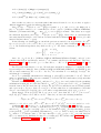
explicit global state. The grammar for processes is described in Figure 1.
4
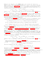
hM,N i ::= x, y, z ∈ V
| p ∈ PN
| n ∈ FN
| f (M1 ,. . . ,Mn ) (f ∈ Σ of arity n)
hP ,Qi ::= 0
| P |Q
| !P
| νn; P
| out(M, N ); P
| in(M, N ); P
| if M =N then P [else Q]
| event F ; P (F ∈ F)
| insert M ,N ; P
| delete M ; P
| lookup M as x in P [else Q]
| lock M ; P
| unlock M ; P
| [L] −[A]→ [R]; P (L, R, A ∈ F ∗ )
Figure 1: Syntax
0 denotes the terminal process. P | Q is the parallel execution of processes P and Q and !P
the replication of P , allowing an unbounded number of sessions in protocol executions. The construct
νn; P binds the name n in P and models the generation of a fresh, random value. Processes out(M, N );
P and in(M, N ); P represent the output, respectively input, of message N on channel M . Readers
familiar with the applied pi calculus [2] may note that we opted for the possibility of pattern matching
in the input construct, rather than merely binding the input to a variable x. The process if M =N
then P else Q will execute P if M =E N and Q otherwise. The event construct is merely used for
annotating processes and will be useful for stating security properties. For readability we sometimes
omit to write else Q when Q is 0, as well as trailing 0 processes.
The remaining constructs are used for manipulating state and are new compared to the applied pi
calculus. We offer two different mechanisms for state. The first construct is functional and allows to
associate a value to a key. The construct insert M ,N binds the value N to a key M . Successive inserts
allow to change this binding. The delete M operation simply “undefines” the mapping for the key M .
The lookup M as x in P else Q allows to retrieve the value associated to M , binding it to the variable
x in P . If the mapping is undefined for M the process behaves as Q. The lock and unlock constructs
allow to gain exclusive access to a resource M . This is essential for writing protocols where parallel
processes may read and update a common memory. We additionally offer another kind of global state
in form of a multiset of ground facts, as opposed to the previously introduced functional store. This
multiset can be altered using the construct [L] −[A]→ [R]; P , which tries to match each fact in the
sequence L to facts in the current multiset and, if successful, adds the corresponding instance of facts
R to the store. The facts A are used as annotations in a similar way to events. The purpose of this
construct is to provide access to the underlying notion of state in tamarin, but we stress that it is
distinct from the previously introduced functional state, and its use is only advised to expert users.
We allow this “low-level” form of state manipulation in addition to the functional state, as it offers a
great flexibility and has shown useful in one of our case studies. This style of state manipulation is
similar to the state extension in the strand space model [17] and the underlying specification language
of the tamarin tool [25, 26]. Note that, even though those stores are distinct (which is a restriction
imposed by our translation), data can be moved from one to another, for example as follows: lookup
’store1’ as x in [] −[ ]→ [store2(x)].
In the following example, which will serve as our running example, we model a security API that,
even though much simplified, illustrates the most salient issues that occur in the analysis of security
5
APIs such as PKCS#11 [13, 10, 15] .
Example. We consider a security device that allows the creation of keys in its secure memory. The
user can access the device via an API. If he creates a key, he obtains a handle, which he can use to
let the device perform operations on his behalf. For each handle the device also stores an attribute
which defines what operations are permitted for this handle. The goal is that the user can never gain
knowledge of the key, as the user’s machine might be compromised. We model the device by the
following process (we use out(m) as a shortcut for out(c, m) for a public channel c):
!Pnew | !Pset | !Pdec | !Pwrap , where
Pnew := νh; νk; event NewKey(h,k);
insert h ‘key’ ,hi,k;
insert h ‘ att ’ ,hi, ‘dec’ ; out(h)
In the first line, the device creates a new handle h and a key k and, by the means of the event
NewKey(h, k), logs the creation of this key. It then stores the key that belongs to the handle by
associating the pair h‘key’, hi to the value of the key k. In the next line, h‘att’, hi is associated to
a public constant ‘dec’. Intuitively, we use the public constants ‘key’ and ‘att’ to distinguish two
databases. The process
Pset := in(h); insert h‘att’,hi, ‘wrap’
allows the attacker to change the attribute of a key from the initial value ‘dec’ to another value ‘wrap’.
If a handle has the ‘dec’ attribute set, it can be used for decryption:
Pdec := in(hh,ci); lookup h‘att’,hi as a in
if a=‘dec’ then
lookup h ‘key’ ,hi as k in
if encCor(c,k)=true then
event DecUsing(k,sdec(c,k));
out(sdec(c,k))
The first lookup stores the value associated to h‘att’, hi in a. The value is compared against ‘dec’. If the
comparison and another lookup for the associated key value k succeeds, we check whether decryption
succeeds and, if so, output the plaintext.
If a key has the ‘wrap’ attribute set, it might be used to encrypt the value of a second key:
Pwrap := in(hh1 ,h2 i); lookup h‘att’,h1 i as a1 in
if a1 =‘wrap’ then
lookup h ‘key’ ,h1 i as k1 in
lookup h ‘key’ , h2 i as k2 in
event Wrap(k1 ,k2 );
out(senc(k2 ,k1 ))
The bound names of a process are those that are bound by νn. We suppose that all names of sort
fresh appearing in the process are under the scope of such a binder. Free names must be of sort pub.
A variable x can be bound in three ways: (i) by the construct lookup M as x, or (ii) x ∈ vars(N )
in the construct in(M, N ) and x is not under the scope of a previous binder, (iii) x ∈ vars(L) in the
construct [L] −[A]→ [R] and x is not under the scope of a previous binder. While the construct lookup
M as x always acts as a binder, the input and [L] −[A]→ [R] constructs do not rebind an already
bound variable but perform pattern matching. For instance in the process
P = in(c,f (x)); in(c,g(x))
x is bound by the first input and pattern matched in the second. It might seem odd that lookup acts
as a binder, while input does not. We justify this decision as follows: as Pdec and Pwrap in the previous
6
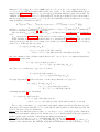
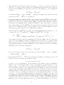
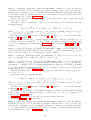
a ∈ FN ∪ PN a ∈
/ ñ
Dname
ν ñ.σ ⊢ a
ν ñ.σ ⊢ t t =E t′
DEq
ν ñ.σ ⊢ t′
x ∈ D(σ)
DFrame
ν ñ.σ ⊢ xσ
ν ñ.σ ⊢ t1 · · · ν ñ.σ ⊢ tn f ∈ Σk
DAppl
ν ñ.σ ⊢ f (t1 , . . . , tn )
Figure 2: Deduction rules.
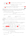
x1 ∈ D(σ)
x2 ∈ D(σ)
ν ñ.σ ⊢ senc(k2 , k1 ) ν ñ.σ ⊢ k1
ν ñ.σ ⊢ sdec(senc(k2 , k1 ), k1 )
sdec(senc(k2 , k1 ), k1 ) =E k2
ν ñ.σ ⊢ k2
Figure 3: Proof tree witnessing that ν ñ.σ ⊢ k2
example show, lookups appear often after input was received. If lookup were to use pattern matching,
the following process
P = in(c, x); lookup ‘store’ as x in P ′
might unexpectedly perform a check if ‘store’ contains the message given by the adversary, instead of
binding the content of ‘store’ to x, due to an undetected clash in the naming of variables.
A process is ground if it does not contain any free variables. We denote by P σ the application of
the homomorphic extension of the substitution σ to P . As usual we suppose that the substitution only
applies to free variables. We sometimes interpret the syntax tree of a process as a term and write P |p
to refer to the subprocess of P at position p (where |, if and lookup are interpreted as binary symbols,
all other constructs as unary).
3.2
Semantics
Frames and deduction Before giving the formal semantics of our calculus we introduce the notions
of frame and deduction. A frame consists of a set of fresh names ñ and a substitution σ and is written
ν ñ.σ. Intuitively a frame represents the sequence of messages that have been observed by an adversary
during a protocol execution and secrets ñ generated by the protocol, a priori unknown to the adversary.
Deduction models the capacity of the adversary to compute new messages from the observed ones.
Definition 1 (Deduction). We define the deduction relation ν ñ.σ ⊢ t as the smallest relation between
frames and terms defined by the deduction rules in Figure 2.
Example. If one key is used to wrap a second key, then, if the intruder learns the first key, he can
deduce the second. For ñ = k1 , k2 and σ = { senc(k2 ,k1 ) /x1 ,k1 /x2 }, ν ñ.σ ⊢ k2 , as witnessed by the proof
tree given in Figure 3.
Operational semantics We can now define the operational semantics of our calculus. The semantics
is defined by a labelled transition relation between process configurations. A process configuration is a
6-tuple (E, S, S MS , P, σ, L) where
• E ⊆ FN is the set of fresh names generated by the processes;
• S : MΣ → MΣ is a partial function modeling the functional store;
• S MS ⊆ G # is a multiset of ground facts and models the multiset of stored facts;
• P is a multiset of ground processes representing the processes executed in parallel;
• σ is a ground substitution modeling the messages output to the environment;
7
Standard operations:
(E, S, S MS , P ∪# {0}, σ, L)
(E, S, S MS , P ∪# {P |Q}, σ, L)
(E, S, S MS , P ∪# {!P }, σ, L)
(E, S, S MS , P ∪# {νa; P }, σ, L)
−→
−→
−→
−→
(E, S, S MS , P, σ, L)
K(M)
(E, S, S MS , P, σ, L)
K(M)
(E, S, S MS , P ∪# {P }, σ ∪ {N /x }, L)
if x is fresh and νE.σ ⊢ M
−−−−→
(E, S, S MS , P ∪# {out(M, N ); P }, σ, L)
(E, S, S MS , P, σ, L)
(E, S, S MS , P ∪# {P, Q}, σ, L)
(E, S, S MS , P ∪# {!P, P }, σ, L)
(E ∪ {a′ }, S, S MS , P ∪# {P {a′ /a}}, σ, L)
if a′ is fresh
−−−−→
if νE.σ ⊢ M
K(hM,N τ i)
(E, S, S MS , P ∪# {in(M, N ); P }, σ, L)
(E, S, S MS , P ∪# {out(M, N ); P, in(M ′ , N ′ ); Q}, σ, L)
if
MS
(E, S, S , P ∪ {if M = N then P else Q}, σ, L)
(E, S, S MS , P ∪ {if M = N then P else Q}, σ, L)
−−−−−−−→ (E, S, S MS , P ∪# {P τ }, σ, L)
if ∃τ. τ is grounding for N, νE.σ ⊢ M, νE.σ ⊢ N τ
−→
(E, S, S MS , P ∪ {P, Qτ }, σ, L)
′
M =E M and ∃τ. N =E N ′ τ and τ grounding for N ′
−→
(E, S, S MS , P ∪ {P }, σ, L) if M =E N
−→
(E, S, S MS , P ∪ {Q}, σ, L) if M 6=E N
F
(E, S, S MS , P ∪ {event(F ); P }, σ, L)
−→
(E, S, S MS , P ∪ {P }, σ, L)
Operations on global state:
(E, S, S MS , P ∪# {insert M, N ; P }, σ, L)
(E, S, S MS , P ∪# {delete M ; P }, σ, L)
(E, S, S MS , P ∪# {lookup M as x in P else Q }, σ, L)
−→ (E, S[M 7→ N ], S MS , P ∪# {P }, σ, L)
−→ (E, S[M 7→ ⊥], S MS , P ∪# {P }, σ, L)
−→ (E, S, S MS , P ∪# {P {V /x}}, σ, L)
if S(N ) =E V is defined and N =E M
MS
−→ (E, S, S , P ∪# {Q}, σ, L)
if S(N ) is undefined for all N =E M
−→ (E, S, S MS , P ∪# {P }, σ, L ∪ { M })
if M 6∈E L
MS
#
′
′
−→ (E, S, S , P ∪ {P }, σ, L \ { M | M =E M })
(E, S, S MS , P ∪# {lookup M as x in P else Q }, σ, L)
(E, S, S MS , P ∪# {lock M ; P }, σ, L)
(E, S, S MS , P ∪# {unlock M ; P }, σ, L)
a′
(E, S, S MS , P ∪# {[l −[a]→ r]; P }, σ, L) −→ (E, S, S MS \ lfacts(l′ ) ∪# r′ , P ∪# { P τ }, σ, L)
if ∃τ, l′ , a′ , r′ . τ grounding for l −[a]→ r, l′ −[a′ ]→ r′ =E (l −[a]→ r)τ,
lfacts(l′ ) ⊆# S MS , pfacts(l′ ) ⊂ S MS
Figure 4: Operational semantics
• L ⊆ MΣ is the set of currently acquired locks.
The transition relation is defined by the rules described in Figure 4. Transitions are labelled by
sets of ground facts. For readability we omit empty sets and brackets around singletons, i.e., we write
∅
f
{f }
→ for −→ and −→ for −→. We write →∗ for the reflexive, transitive closure of → (the transitions
f
f
that are labelled by the empty sets) and write ⇒ for →∗ →→∗ . We can now define the set of traces,
i.e., possible executions, that a process admits.
Definition 2 (Traces of P ). Given a ground process P we define the set of traces of P as
n
traces pi (P ) = [F1 , . . . , Fn ] | (∅, ∅, ∅, {P }, ∅, ∅)
F
1
=⇒
(E1 , S1 , S1MS , P1 , σ1 , L1 )
o
F2
Fn
=⇒
. . . =⇒
(En , Sn , SnMS , Pn , σn , Ln )
Example. In Figure 5 we display the transitions that illustrate how the first key is created on the
security device in our running example and witness that [NewKey(h′ , k′ )] ∈ traces pi (P ).
8
(∅, ∅, ∅, { !Pnew , !Pset |!Pdec |!Pwrap }# , ∅, ∅) → (∅, ∅, ∅, { Pnew }# ∪# P ′ , ∅, ∅)
{z
}
|
=:P ′
→ (∅, ∅, ∅, { ν h; νk; event NewKey(h, k); . . . }# ∪# P ′ , ∅, ∅)
→∗ ({ h′ , k′ }, ∅, ∅, { event NewKey(h′ , k′ ); . . . }# ∪# P ′ , ∅, ∅)
NewKey(h′ ,k ′ )
−−−−−−−−−→ ({ h′ , k′ }, ∅, ∅, { insert h‘key’, h′ i, k′ ; . . . }# ∪# P ′ , ∅, ∅)
′
→∗ ({ h′ , k′ }, S, ∅, { out(h′ ); 0 }# ∪# P ′ , ∅, ∅) →∗ ({ h′ , k′ }, S, ∅, P ′ , { h /x1 }, ∅)
where S(h‘key’,h′ i) = k′ and S(h‘att’,h′ i) = ‘dec’.
Figure 5: Example of transitions modelling the creation of a key on a PKCS#11-like device
4
Labelled multiset rewriting
We now recall the syntax and semantics of labelled multiset rewriting rules, which constitute the input
language of the tamarin tool [25].
Definition 3 (Multiset rewrite rule). A labelled multiset rewrite rule ri is a triple (l, a, r), l, a, r ∈
F ∗ , written l −[a]→ r. We call l = prems(ri ) the premises, a = actions(ri ) the actions, and r =
conclusions(ri ) the conclusions of the rule.
Definition 4 (Labelled multiset rewriting system). A labelled multiset rewriting system is a set of
labelled multiset rewrite rules R, such that each rule l −[a]→ r ∈ R satisfies the following conditions:
• l, a, r do not contain fresh names
• r does not contain Fr-facts
A labelled multiset rewriting system is called well-formed, if additionally
• for each l′ −[a′ ]→ r ′ ∈E ginsts(l −[a]→ r) we have that ∩r′′ =E r′ names(r ′′ )∩FN ⊆ ∩l′′ =E l′ names(l′′ )∩
FN .
We define one distinguished rule Fresh which is the only rule allowed to have Fr-facts on the
right-hand side
Fresh : [] −[]→ [Fr(x : fresh)]
The semantics of the rules is defined by a labelled transition relation.
Definition 5 (Labelled transition relation). Given a multiset rewriting system R we define the labeled
transition relation →R ⊆ G # × P(G) × G # as
a
S −→R ((S \# lfacts(l)) ∪# r)
if and only if l −[a]→ r ∈E ginsts(R ∪ Fresh), lfacts(l) ⊆# S and pfacts(l) ⊆ S.
Definition 6 (Executions). Given a multiset rewriting system R we define its set of executions as
n
A1
An
exec msr (R) = ∅ −→
R . . . −→R Sn |
∀a, i, j : 0 ≤ i 6= j < n.
(Si+1 \# Si ) = {Fr(a)} ⇒ (Sj+1 \# Sj ) 6= {Fr(a)}
The set of executions consists of transition sequences that respect freshness, i. e., for a given name
a the fact Fr(a) is only added once, or in other words the rule Fresh is at most fired once for each
name. We define the set of traces in a similar way as for processes.
9
Definition 7 (Traces). The set of traces is defined as
n
traces msr (R) = [A1 , . . . , An ] | ∀ 0 ≤ i ≤ n. Ai 6= ∅
o
A1
An
msr (R)
and ∅ =⇒
R . . . =⇒R Sn ∈ exec
A
∅
A
∅
where =⇒R is defined as −→ ∗R −→ R −→ ∗R .
Note that both for processes and multiset rewrite rules the set of traces is a sequence of sets of
facts.
5
Security Properties
In the tamarin tool [25] security properties are described in an expressive two-sorted first-order logic.
The sort temp is used for time points, Vtemp are the temporal variables.
Definition 8 (Trace formulas). A trace atom is either false ⊥, a term equality t1 ≈ t2 , a timepoint
.
ordering i ⋖ j, a timepoint equality i = j, or an action F @i for a fact F ∈ F and a timepoint i. A
trace formula is a first-order formula over trace atoms.
As we will see in our case studies this logic is expressive enough to analyze a variety of security
properties, including complex injective correspondence properties.
To define the semantics, let each sort s have a domain D(s). D(temp) = Q, D(msg ) = M,
D(fresh) = FN , and D(pub) = PN . A function θ : V → M ∪ Q is a valuation if it respects sorts, that
is, θ(Vs ) ⊂ D(s) for all sorts s. If t is a term, tθ is the application of the homomorphic extension of θ
to t.
Definition 9 (Satisfaction relation). The satisfaction relation (tr , θ) ϕ between trace tr , valuation
θ and trace formula ϕ is defined as follows:
(tr , θ) ⊥
(tr , θ) F @i
(tr , θ) i ⋖ j
.
(tr , θ) i = j
(tr , θ) t1 ≈ t2
(tr , θ) ¬ϕ
(tr , θ) ϕ1 ∧ ϕ2
(tr , θ) ∃x : s.ϕ
never
iff θ(i) ∈ idx (tr) and F θ ∈E tr θ(i)
iff θ(i) < θ(j)
iff θ(i) = θ(j)
iff t1 θ =E t2 θ
iff not (tr , θ) ϕ
iff (tr , θ) ϕ1 and (tr , θ) ϕ2
iff there is u ∈ D(s) such that
(tr , θ[x 7→ u]) ϕ
When ϕ is a ground formula we sometimes simply write tr ϕ as the satisfaction of ϕ is independent
of the valuation.
Definition 10 (Validity, satisfiability). Let Tr ⊆ (P(G))∗ be a set of traces. A trace formula ϕ is
said to be valid for Tr , written Tr ∀ ϕ, if for any trace tr ∈ Tr and any valuation θ we have that
(tr , θ) ϕ.
A trace formula ϕ is said to be satisfiable for Tr , written Tr ∃ ϕ, if there exist a trace tr ∈ Tr
and a valuation θ such that (tr , θ) ϕ.
Note that Tr ∀ ϕ iff Tr 6∃ ¬ϕ. Given a multiset rewriting system R we say that ϕ is valid, written
R ∀ ϕ, if traces msr (R) ∀ ϕ. We say that ϕ is satisfied in R, written R ∃ ϕ, if traces msr (R) ∃ ϕ.
Similarly, given a ground process P we say that ϕ is valid, written P ∀ ϕ, if traces pi (P ) ∀ ϕ, and
that ϕ is satisfied in P , written P ∃ ϕ, if traces pi (P ) ∃ ϕ.
Example. The following trace formula expresses secrecy of keys generated on the security API, which
we introduced in Section 3.
¬(∃h, k : msg, i, j : temp. NewKey(h, k)@i ∧ K(k)@j)
10
Out(x)
−[ ]→
!K(x) −[K(x)]→
−[ ]→
Fr(x : fresh)
−[ ]→
!K(x1 ), . . . , !K(xk )
−[ ]→
!K(x)
(MDOut)
In(x)
(MDIn)
!K(x : pub)
(MDPub)
!K(x : fresh)
(MDFresh)
k
!K(f (x1 , . . . , xk )) for f ∈ Σ
(MDAppl)
Figure 6: The set of rules MD.
6
A translation from processes into multiset rewrite rules
In this section we define a translation from a process P into a set of multiset rewrite rules JP K and a
translation on trace formulas such that P |=∀ ϕ if and only if JP K |=∀ JϕK. Note that the result also
holds for satisfiability, as an immediate consequence. For a rather expressive subset of trace formulas
(see [25] for the exact definition of the fragment), checking whether JP K |=∀ JϕK can then be discharged
to the tamarin prover that we use as a backend.
6.1
Definition of the translation of processes
To model the adversary’s message deduction capabilities, we introduce the set of rules MD defined in
Figure 6.
In order for our translation to be correct, we need to make some assumptions on the set of processes
we allow. These assumptions are however, as we will see, rather mild and most of them without loss
of generality. First we define a set of reserved variables that will be used in our translation and whose
use we therefore forbid in the processes.
Definition 11 (Reserved variables and facts). The set of reserved variables is defined as the set
containing the elements na for any a ∈ FN and lock l for any l ∈ N.
The set of reserved facts Fres is defined as the set containing facts f (t1 , . . . , tn ) where t1 , . . . , tn ∈ T
and f ∈ { Init, Insert, Delete, IsIn, IsNotSet, state, Lock, Unlock, Out, Fr, In, Msg, ProtoNonce, Eq,
NotEq, Event, InEvent }.
Similar to [3], for our translation to be sound, we require that for each process, there exists an
injective mapping assigning to every unlock t in a process a lock t that precedes it in the process’
syntax tree. Moreover, given a process lock t; P the corresponding unlock in P may not be under a
parallel or replication. These conditions allow us to annotate each corresponding pair lock t, unlock t
with a unique label l. The annotated version of a process P is denoted P . The formal definition of P
is given in Appendix A. In case the annotation fails, i.e., P violates one of the above conditions, the
process P contains ⊥.
Definition 12 (well-formed). A ground process P is well-formed if
• no reserved variable nor reserved fact appear in P ,
• any name and variable in P is bound at most once and
• P does not contain ⊥.
• For each action l −[a]→ r that appears in the process, the following holds: for each l′ −[a′ ]→ r ′ ∈E
ginsts(l −[a]→ r) we have that ∩r′′ =E r′ names(r ′′ ) ∩ FN ⊆ ∩l′′ =E l′ names(l′′ ) ∩ FN .
A trace formula ϕ is well-formed if no reserved variable nor reserved fact appear in ϕ.
The two first restrictions of well-formed processes are not a loss of generality as processes and
formulas can be consistently renamed to avoid reserved variables and α-converted to avoid binding
names or variables several times. Also note that the second condition is not necessarily preserved
during an execution, e.g. when unfolding a replication, !P and P may bind the same names. We only
require this condition to hold on the initial process for our translation to be correct.
11
The annotation of locks restricts the set of protocols we can translate, but allows us to obtain better
verification results, since we can predict which unlock is “supposed” to close a given lock. This additional
information is helpful for tamarin’s backward reasoning. We think that our locking mechanism captures
all practical use cases. Using our calculus’ “low-level” multiset manipulation construct, the user is also
free to implement locks himself, e.g., as
[NotLocked()] → []; code ; [] → [NotLocked()]
(In this case the user does not benefit from the optimisation we put into the translation of locks.)
Obviously, locks can be modelled both in tamarin’s multiset rewriting calculus (this is actually what
the translation does) and Mödersheim’s set rewriting calculus [22]. However, protocol steps typically
consist of a single input, followed by several database lookups, and finally an output. In practice, they
tend to be modelled as a single rule, and are therefore atomic. Real implementations are however
different, as several entities might be involved, database lookups could be slow, etc. In this case, such
simplified models could, e. g., miss race conditions. To the best of our knowledge, StatVerif is the only
comparable tool that models locks explicitly and it has stronger restrictions.
Definition 13. Given a well-formed ground process P we define the labelled multiset rewriting system
JP K as
MD ∪ {Init} ∪ JP , [], []K
• where the rule Init is defined as
Init : [] −[Init()]→ [state[] ()]
• JP, p, x̃K is defined inductively for process P , position p ∈ N∗ and sequence of variables x̃ in
Figure 7.
• For a position p of P we define statep to be persistent if P |p = !Q for some process Q; otherwise
statep is linear.
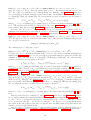
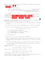
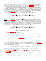
In the definition of JP, p, x̃K we intuitively use the family of facts statep to indicate that the process
is currently at position p in its syntax tree. A fact statep will indeed be true in an execution of these
rules whenever some instance of Pp (i.e. the process defined by the subtree at position p of the syntax
tree of P ) is in the multiset P of the process configuration. The translation of the zero-process, parallel
and replication operators merely use statep -facts. For instance JP | Q, p, x̃K defines the rule
[statep (x̃)] → [statep·1 (x̃), statep·2 (x̃)]
which intuitively states that when a process is at position p (modelled by the fact statep (x̃) being true)
then the process is allowed to move both to P (putting statep·1 (x̃) to true) and Q (putting statep·2 (x̃) to
true). The translation of JP | Q, p, x̃K also contains the set of rules JP, p · 1, x̃K ∪ JQ, p · 2, x̃K expressing
that after this transition the process may behave as P and Q, i.e., the processes at positions p · 1,
respectively p · 2, in the process tree. Also note that the translation of !P results in a persistent fact
as !P always remains in P. The translation of the construct ν a translates the name a into a variable
na , as msr rules must not contain fresh names. Any instantiation of this rule will substitute na by
a fresh name, which the Fr-fact in the premise guarantees to be new. This step is annotated with a
(reserved) action ProtoNonce, used in the proof of correctness to distinguish adversary and protocol
nonces. Note that the fact statep·1 in the conclusion carries na , so that the following protocol steps
are bound to the fresh name used to instantiate na . The first rules of the translation of out and in
model the communication between the protocol and the adversary, and vice versa. In the case of
out, the adversary must know the channel M , modelled by the fact In(M ) in the rule’s premisse, and
learns the output message, modelled by the fact Out(N ) in the conclusion. In the case of in, the
knowledge of the message N is additionally required and the variables of the input message are added
to the parameters of the state fact to reflect that these variables are bound. The second and third
rules of the translations of out and in model an internal communication, which is synchronous. For
12
J0, p, x̃K = {[statep (x̃)] → []}
JP | Q, p, x̃K = {[statep (x̃)] → [statep·1 (x̃), statep·2 (x̃)]} ∪ JP, p · 1, x̃K ∪ JQ, p · 2, x̃K
J!P, p, x̃K = {[!statep (x̃)] → [statep·1 (x̃)]} ∪ JP, p · 1, x̃K
Jνa; P, p, x̃K = {[statep (x̃), Fr(na : fresh)] −[ProtoNonce (na : fresh)]→ [statep·1 (x̃, na : fresh)]}
∪ JP, p · 1, (x̃, na : fresh)K
JOut(M, N ); P, p, x̃K = {[statep (x̃), In(M )] −[InEvent(M )]→ [Out(N ), statep·1 (x̃)],
[statep (x̃)] → [Msg(M, N ), statesemi
(x̃)],
p
[statesemi
p (x̃), Ack(M, N )] → [statep·1 (x̃)] } ∪ JP, p · 1, x̃K
JIn(M, N ); P, p, x̃K = {[statep (x̃), In(hM, N i)] −[InEvent(hM, N i)]→ [statep·1 (x̃ ∪ vars(N ))],
[statep (x̃), Msg(M, N )] → [statep·1 (x̃ ∪ vars(N )), Ack(M, N )]}
∪ JP, p · 1, x̃ ∪ vars(N )K
Jif M = N then P = {[statep (x̃)] −[ Eq(M, N ) ]→ [statep·1 (x̃)],
else Q, p, x̃K
[statep (x̃)] −[NotEq(M, N )]→ [statep·2 (x̃)]}
∪ JP, p · 1, x̃K ∪ JQ, p · 2, x̃K
Jevent F ; P, p, x̃K = {[statep (x̃)] −[Event(), F ]→ [statep·1 (x̃)]} ∪ JP, p · 1, x̃K
Jinsert s, t; P, p, x̃K = {[statep (x̃)] −[Insert(s, t)]→ [statep·1 (x̃)]} ∪ JP, p · 1, x̃K
Jdelete s; P, p, x̃K = {[statep (x̃)] −[Delete(s)]→ [statep·1 (x̃)]} ∪ JP, p · 1, x̃K
Jlookup M as v = {[statep (x̃)] −[IsIn(M, v)]→ [statep·1 (M̃ , v)],
in P else Q, p, x̃K
[statep (x̃)] −[IsNotSet(M )]→ [statep·2 (x̃)]}
∪ JP, p · 1, (x̃, v)K ∪ JQ, p · 2, x̃K
l
Jlock s; P, p, x̃K = {[Fr(lockl ), statep (x̃)] −[Lock(lock l , s)]→ [statep·1 (x̃, lock l )]}
∪ JP, p · 1, x̃K
l
Junlock s; P, p, x̃K = {[statep (x̃)] −[Unlock(lock l , s)]→ [statep·1 (x̃)]} ∪ JP, p · 1, x̃K
J[l −[a]→ r]; P, p, x̃K = {[statep (x̃), l] −[Event(), a]→ [r, statep·1 (x̃ ∪ vars(l))]}
∪ JP, p · 1, x̃ ∪ vars(l)K
Figure 7: Translation of processes: definition of JP, p, x̃K
13
[]
−[Init()]→
[state[] ()]
[state[] ()]
−[ ]→
[!state[1] ()]
[!state[1] (), Fr(h)]
−[ ]→
[state[11] (h)]
[state[11] (h), Fr(k)]
−[ ]→
[state[111] (k, h)]
[state[111] (k, h)] −[Event(), NewKey(h, k)]→ [state[1111] (k, h)]
[state[1111] (k, h)] −[Insert(h’key’, hi, k)]→ [state[11111] (k, h)]
[state[11111] (k, h)] −[Insert(h’att’, hi, ’dec’)]→ [state[111111] (k, h)]
[state[111111] (k, h)]
−[ ]→
[Out(h), state[1111111] (k, h)]
Figure 8: The set of multiset rewrite rules J!Pnew K (omitting the rules in MD)
this reason, when the second rule of the translation of out is fired, the state-fact is substituted by an
intermediate, semi-state fact, statesemi , reflecting that the sending process can only execute the next
step if the message was successfully received. The fact Msg(M, N ) models that a message is present on
the synchronous channel. Only with the acknowledgement fact Ack(M, N ), resulting from the second
rule of the translation of in, is it possible to advance the execution of the sending process, using the
third rule in the translation of out, which transforms the semi-state and the acknowledgement of receipt
into statep·1 (. . .). Only now the next step in the execution of the sending process can be executed. The
remaining rules essentially update the position in the state facts and add labels. Some of these labels
are used to restrict the set of executions. For instance the label Eq(M ,N ) will be used to indicate that
we only consider executions in which M =E N . As we will see in the next section these restrictions
will be encoded in the trace formula.
Example. Figure 8 illustrates the above translation by presenting the set of msr rules J!Pnew K (omitting
the rules in MD already shown in Figure 6).
A graph representation of an example trace, generated by the tamarin tool, is depicted in Figure 9.
Every box in this picture stands for the application of a multiset rewrite rule, where the premises are at
the top, the conclusions at the bottom, and the actions (if any) in the middle. Every premise needs to
have a matching conclusion, visualized by the arrows, to ensure the graph depicts a valid msr execution.
(This is a simplification of the dependency graph representation tamarin uses to perform backwardinduction [25, 26].) Note that the machine notation for statep () predicates omits brackets [ ] in the
position p and denotes the empty sequence by ‘0’. We also note that in the current example !state[1] ()
is persistent and can therefore be used multiple times as a premise. As Fr( ) facts are generated by
the Fresh rule which has an empty premise and action, we omit instances of Fresh and leave those
premises, but only those, disconnected.
Remark 1. One may note that, while for all other operators, the translation produces well-formed multiset rewriting rules (as long as the process is well-formed itself ), this is not the case for the translation
of the lookup operator, i. e., it violates the well-formedness condition from Definition 4. Tamarin’s constraint solving algorithm requires all rules, with the exception of Fresh, to be well-formed. We show
however that, under these specific conditions, the solution procedure is still correct. See Appendix B
for the proof.
6.2
Definition of the translation of trace formulas
We can now define the translation for formulas.
Definition 14. Given a well-formed trace formula ϕ we define
JϕK∀ := α ⇒ ϕ
and
JϕK∃ := α ∧ ϕ
where α is defined in Figure 10.
The formula α uses the actions of the generated rules to filter out executions that we wish to
discard:
14
0[Init( )]
state_0( )
state_0( )
!state_01( )
!state_01( )
Fr( h )
state_011( h )
state_011( h )
!state_01( )
Fr( h’ )
state_011( h’ )
Fr( k )
state_011( h’ )
state_0111( k, h )
Fr( k’ )
state_0111( k’, h’ )
state_0111( k, h )
state_0111( k’, h’ )
Event( ),NewKey( h, k )
Event( ),NewKey( h’, k’ )
state_01111( k, h )
state_01111( k’, h’ )
state_01111( k, h )
state_01111( k’, h’ )
Insert( <’key’, h>, k )
Insert( <’key’, h’>, k’ )
state_011111( k, h )
state_011111( k’, h’ )
state_011111( k, h )
state_011111( k’, h’ )
Insert( <’att’, h>, ’dec’ )
Insert( <’att’, h’>, ’dec’ )
state_0111111( k, h )
state_0111111( k’, h’ )
state_0111111( k, h )
Out( h )
state_0111111( k’, h’ )
state_01111111( k, h )
Out( h’ )
state_01111111( k’, h’ )
Figure 9: Example trace for the translation of !Pnew .
• αinit ensures that the init rule is only fired once.
• αeq and αnoteq ensure that we only consider traces where all (dis)equalities hold.
• αin and αnotin ensure that a successful lookup was preceded by an insert that was neither revoked
nor overwritten while an unsuccessful lookup was either never inserted, or deleted and never reinserted.
• αlock checks that between each two matching locks there must be an unlock. Furthermore,
between the first of these locks and the corresponding unlock, there is neither a lock nor an
unlock.
• αinev ensures that whenever an instance of MDIn is required to generate an In-fact, it is generated
as late as possible, i. e., there is no visible event between the action K(t) produced by MDIn,
and a rule that requires In(t).
We also note that Tr ∀ JϕK∀ iff Tr 6∃ J¬ϕK∃ .
The axioms in the translation of the formula are designed to work hand in hand with the translation
of the process into rules. They express the correctness of traces with respect to our calculus’ semantics,
but are also meant to guide tamarin’s constraint solving algorithm. αin and αnotin illustrate what kind
of axioms work well: when a node with the action IsIn is created, by definition of the translation, this
corresponds to a lookup command. The existential translates into a graph constraint that postulates
an insert node for the value fetched by the lookup, and three formulas assuring that a) this insert node
appears before the lookup, b) is uniquely defined, i. e., it is the last insert to the corresponding key,
and c) there is no delete in between. Due to these conditions, αnotin only adds one Insert node per IsIn
node – the case where an axiom postulates a node, which itself allows for postulating yet another node
needs to be avoided, as tamarin runs into loops otherwise. Similarly, a naïve way of implementing
locks using an axiom would postulate that every lock is preceeded by an unlock and no lock or unlock
15
α := αinit ∧ αeq ∧ αnoteq ∧ αin ∧ αnotin ∧ αlock ∧ αinev and
Init()@i ∧ Init()@j =⇒ i = j
αinit :=∀i, j.
αeq :=∀x, y, i.
αnoteq :=∀x, y, i.
αin :=∀x, y, t3 .
Eq(x, y)@i =⇒ x ≈ y
NotEq(x, y)@i =⇒ ¬(x ≈ y)
IsIn(x, y)@t3 =⇒ ∃t2 . Insert(x, y)@t2 ∧ t2 ⋖ t3
.
∧ ∀t1 , y. Insert(x, y)@t1 =⇒ (t1 ⋖ t2 ∨ t1 = t2 ∨ t3 ⋖ t1 )
∧ ∀t1 .
αnotin :=∀x, y, t3 .
Delete(x)@t1 =⇒ (t1 ⋖ t2 ∨ t3 ⋖ t1 )
IsNotSet(x)@t3 =⇒ (∀t1 , y. Insert(x, y)@t1 =⇒ t3 ⋖ t1 )∨
(∃t1 . Delete(x)@t1 ∧ t1 ⋖ t3
∧ ∀t2 , y. (Insert(x, y)@t2 ∧ t2 ⋖ t3 ) =⇒ t2 ⋖ t1 )
′
′
αlock :=∀x, l, l , i, j. Lock(l, x)@i ∧ Lock(l , x)@j ∧ i ⋖ j
=⇒ ∃k. Unlock(l, x)@k ∧ i ⋖ k ∧ k ⋖ j
∧ (∀l′ , m. Lock(l′ , x)@m =⇒ ¬(i ⋖ m ∧ m ⋖ k))
∧ (∀l′ , m. Unlock(l′ , x)@m =⇒ ¬(i ⋖ m ∧ m ⋖ k))
αinev :=∀t, i.
InEvent(t)@i =⇒ ∃j. K(t)@j ∧ (∀k. Event()@k =⇒ (k ⋖ j ∨ i ⋖ k))
∧ (∀k, t′ . K(t′ )@k =⇒ (k ⋖ j ∨ i ⋖ k ∨ k ≈ j))
Figure 10: Definition of α.
in between, unless it is the first lock. This again would cause tamarin to loop, because an unlock is
typically preceeded by yet another lock. The axiom αlock avoids this caveat because it only applies to
pairs of locks carrying the same annotations.
We will outline how αlock is applied during the constraint solving procedure:
1. If there are two locks for the same term and with possibly different annotations, an unlock for
the first of those locks is postulated, more precisely, an unlock with the same term, the same
annotation and no lock or unlock for the same term in-between. The axiom itself contains only
one case, so the only case distinction that takes place is over which rule produces the matching
Unlock-action. However, due to the annotation, all but one are refuted immediately in the next
step. Note further that αlock postulates only a single node, namely the node with the action
Unlock.
2. Due to the annotation, the fact statep (. . .) contains the fresh name that instantiates the annotation variable. Let a : fresh be this fresh name. Every fact statep′ (. . .) for some position p′ that
is a prefix of p and a suffix of the position of the corresponding lock contains this fresh name.
Furthermore, every rule instantiation that is an ancestor of a node in the dependency graph
corresponds to the execution of a command that is an ancestor in the process tree. Therefore,
the backward search eventually reaches the matching lock, including the annotation, which is
determined to be a, and hence appears in the Fr-premise.
3. Because of the Fr-premise, any existing subgraph that already contains the first of the two original
locks would be merged with the subgraph resulting from the backwards search that we described
in the previous step, as otherwise Fr(a) would be added at two different points in the execution.
4. The result is a sequence of nodes from the first lock to the corresponding unlock, and graph
constraints restricting the second lock to not take place between the first lock and the unlock.
We note that the axiom αlock is only instantiated once per pair of locks, since it requires that
i ⋖ j, thereby fixing their order.
In summary, the annotation helps distinguishing which unlock is expected between to locks, vastly
improving the speed of the backward search. This optimisation, however, required us to put restrictions
on the locks.
16
6.3
Correctness of the translation
The correctness of our translation is stated by the following theorem.
Theorem 1. Given a well-formed ground process P and a well-formed trace formula ϕ we have that
traces pi (P ) ⋆ ϕ iff traces msr (JP K) ⋆ JϕK⋆
where ⋆ is either ∀ or ∃.
We here give an overview of the main propositions and lemmas needed to prove Theorem 1. To
show the result we need two additional definitions. We first define an operation that allows to restrict
a set of traces to those that satisfy the trace formula α as defined in Definition 14.
Definition 15. Let α be the trace formula as defined in Definition 14 and Tr a set of traces. We
define
filter (Tr ) := {tr ∈ Tr | ∀θ.(tr, θ) α}
The following proposition states that if a set of traces satisfies the translated formula then the
filtered traces satisfy the original formula.
Proposition 1. Let Tr be a set of traces and ϕ a trace formula. We have that
Tr ⋆ JϕK⋆ iff filter (Tr ) ⋆ ϕ
where ⋆ is either ∀ or ∃.
The proof (detailed in Appendix) follows directly from the definitions. Next we define the hiding
operation which removes all reserved facts from a trace.
Definition 16 (hide). Given a trace tr and a set of facts F we inductively define hide([]) = [] and
(
hide(tr )
if F ⊆ Fres
hide(F · tr ) :=
(F \ Fres ) · hide(tr ) otherwise
Given a set of traces Tr we define hide(Tr ) = {hide(t) | t ∈ Tr }.
As expected well-formed formulas that do not contain reserved facts evaluate the same whether
reserved facts are hidden or not.
Proposition 2. Let Tr be a set of traces and ϕ a well-formed trace formula. We have that
Tr ⋆ ϕ iff hide(Tr ) ⋆ ϕ
where ⋆ is either ∀ or ∃.
We can now state our main lemma which is relating the set of traces of a process P and the set of
traces of its translation into multiset rewrite rules (proven in the full version).
Lemma 1. Let P be a well-formed ground process. We have that
traces pi (P ) = hide(filter (traces msr (JP K))).
Our main theorem can now be proven by applying Lemma 1, Proposition 3 and Proposition 1.
Proof of Theorem 1.
traces pi (P ) ⋆ ϕ
⇔ hide(filter (traces msr (JP K))) ⋆ ϕ
by Lemma 1
⇔ filter (traces msr (JP K)) ⋆ ϕ
by Proposition 3
⇔ traces msr (JP K) ⋆ JϕK⋆
by Proposition 1
17
7
Case studies
In this section we briefly overview some case studies we performed. These case studies include a simple
security API similar to PKCS#11 [23], the Yubikey security token, the optimistic contract signing
protocol by Garay, Jakobsson and MacKenzie (GJM) [16] and a few other examples discussed in
Arapinis et al. [3] and Mödersheim [22]. The results are summarized in Figure 11. For each case study
we provide the number of typing lemmas that were needed by the tamarin prover and whether manual
guidance of the tool was required. In case no manual guidance is required we also give execution times.
We do not detail all the formal models of the protocols and properties that we studied, and sometimes
present slightly simplified versions. All files of our prototype implementation and our case studies are
available at http://sapic.gforge.inria.fr/.
Example
Security API à la PKCS#11
Yubikey Protocol [19, 28]
GJM protocol [3, 16]
Mödersheim’s example (locks/inserts) [22]
Mödersheim’s example (embedded msr rules) [22]
Security Device [3]
Needham-Schroeder-Lowe [21]
∗
Typing Lemmas
1
3
0
0
0
1
1
Automated Run∗
yes (51s)
no
yes (36s)
no∗∗
yes (1s)
yes (21s)
yes (5s)
(Running times on Intel Core2 Duo 2.66Ghz with 4GB RAM)
∗∗
(little interaction: 7 manual rule selections)
Figure 11: Case studies.
7.1
Security API à la PKCS#11
This example illustrates how our modelling might be useful for the analysis of Security APIs in the
style of the PKCS#11 standard [23]. We expect studying a complete model of PKCS#11, such as
in [13], to be a straightforward extension of this example. In addition to the processes presented in the
running example in Section 3 the actual case study models the following two operations: (i) encryption:
given a handle and a plain-text, the user can request an encryption under the key the handle points
to. (ii) unwrap given a ciphertext senc(k2 , k1 ), and a handle h1 , the user can request the ciphertext
to be unwrapped, i.e. decrypted, under the key pointed to by h1 . If decryption is successful the result
is stored on the device, and a handle pointing to k2 is returned. Moreover, contrary to the running
example, at creation time keys are assigned the attribute ‘init’, from which they can move to either
‘wrap’, or ‘unwrap’, see the following snippet:
in (h ‘set_dec’,hi) ; lock h ‘ att ’ ,hi;
2
lookup h ‘ att ’ ,hi as a in
3
if a=‘init ’ then
4
insert h ‘ att ’ ,hi, ‘dec’ ; unlock h ‘ att ’ ,hi
1
Note that, in contrast to the running example, it is necessary to encapsulate the state changes between
lock and unlock. Otherwise an adversary can stop the execution after line 3, set the attribute to ‘wrap’
in a concurrent process and produce a wrapping. After resuming operation at line 4, he can set the
key’s attribute to ‘dec’, even though the attribute is set to ‘wrap’. Hence, the attacker is allowed to
decrypt the wrapping he has produced and can obtain the key. Such subtleties can produce attacks
that our modeling allows to detect. If locking is handled correctly, we show secrecy of keys produced
on the device, proving the property introduced in Example 5. If locks are removed the attack described
before is found.
18
7.2
Yubikey
The Yubikey [28] is a small hardware device designed to authenticate a user against network-based
services. Manufactured by Yubico, a Swedish company, the Yubikey itself is a low cost ($25), thumbsized USB device. In its typical configuration, it generates one-time passwords based on encryptions
of a secret value, a running counter and some random values using a unique AES-128 key contained in
the device. The Yubikey authentication server accepts a one-time password only if it decrypts under
the correct AES key to a valid secret value containing a counter larger than the last counter accepted.
The counter is thus used as a means to prevent replay attacks. To date, over a million Yubikeys have
been shipped to more than 30,000 customers including governments, universities and enterprises, e.g.
Google, Microsoft, Agfa and Symantec [29].
Besides the counter values used in the one-time password, the Yubikey stores three additional
pieces of information: the public id pid that is used to identify the Yubikey, a secret id secretid that
is transmitted as part of the one-time password and only known to the server and the Yubikey, as well
as the AES key k, which is also shared with the server. The following process PYubikey models a single
Yubikey, as well as its initial configuration, where an entry in the server’s database for the public id
pid is created. This entry contains a tuple consisting of the Yubikey’s secret id, AES key, and an initial
counter value.
PYubikey =
ν k; ν pid; ν secretid ;
insert h ‘ Server ’ , pidi , h secretid , k, ‘ zero ’ i ;
insert h ‘Yubikey’, pidi , ‘ zero ’+‘one’;
out(pid) ;
!PPlugin | !PButtonPress
Here, the processes !PPlugin and !PButtonPress model the Yubikey being unplugged and plugged in again
(possibly on a different computer), and the emission of the one-time password. We will only discuss
PButtonPress here. When the user presses the button on the Yubikey, the device outputs a one-time
password consisting of a counter tc, the secret id secretid and additional randomness npr encrypted
using the AES key k.
PButtonPress =
lock pid;
lookup h ‘Yubikey’,pidi as tc in
insert h ‘Yubikey’,pidi , tc + ‘one’;
ν nonce; ν npr;
event YubiPress(pid, secretid ,k, tc) ;
out(hpid,nonce,senc(h secretid , tc ,npri,k)i) ;
unlock pid
The one-time password senc(hsecretid, tc, npri, k) can be used to authenticate against a server that
shares the same secret key, which we model in the process PServer . The process receives the encrypted
one-time password along with the public id pid of a Yubikey and a nonce that is part of the protocol,
but is irrelevant for the authentication of the Yubikey on the server.
The server looks up the secret id and the AES key associated to the public id, i. e., to the Yubikey
sending the request, as well as the last recorded counter value otc. If the key and secret id used in the
request match the values retrieved from the database, then the event Smaller(otc, tc) is logged along
with the event Login(pid , k, tc), which marks a successful login of the Yubikey pid with key k for the
counter value tc. Afterwards, the old tuple hsecretid , k, otci is replaced by hsecretid , k, tci, to update
the latest counter value received.
PServer =
! in(hpid,nonce,senc(h secretid , tc ,npri,k)i) ;
lock pid;
lookup h ‘ Server ’ , pidi as tuple in
if fst ( tuple )=secretid then
19
if fst (snd(tuple ))=k then
event Smaller(snd(snd(tuple )) , tc)
event Login(pid,k, tc ) ;
insert h ‘ Server ’ ,pidi , h secretid ,k, tci ;
unlock pid
Note that, in our modelling, the server keeps one lock per public id, which means that it is possible
to have several active instances of the server thread in parallel as long as all requests concern different
Yubikeys.
An important part of the modelling of the protocol is to determine whether one counter value is
smaller than another. To this end, our modelling employs a feature added to the development version
of tamarin as of October 2012, a union operator ∪# for multisets of message terms. The operator is
denoted with a plus sign (“+”). We model the counter as a multiset only consisting of the symbols
“one” and “zero”. The multiplicity of ‘one’ in the multiset is the value of the counter. A counter value
is considered smaller than another one, if the first multiset is included in the second. A test a < b is
included by adding the event Smaller(a, b) and an axiom that requires that a is a subset of b:
αSmaller :=∀i : temp, a, b : msg. Smaller(a, b)@i
⇒ ∃z : msg . a + z = b
We incorporate this axiom into the security properties just like in Definition 14. Intuitively, we are
only interested in traces where a is indeed smaller than b.
The process we analyse models a single authentication server (that may run arbitrary many threads)
and an arbitrary number of Yubikeys, i. e., PServer | !PYubikey . Among other properties, we show by
the means of an injective correspondence property that an attacker that controls the network cannot
perform replay attacks, and that each successful login was preceded by a user “pressing the button”,
formally:
∀ pid , k, x, t2 .Login(pid, k , x )@t2 ⇒
∃sid, t1 .YubiPress(pid, sid, k , x )@t1 ∧ t1 ⋖ t2
∧ ∀t3 .Login(pid, k , x )@t3 ⇒ t3 = t2
Besides injective correspondence, we show the absence of replay attacks and the property that a
successful login invalidates previously emitted one-time passwords. All three properties follow more or
less directly from a stronger invariant, which itself can be proven in 295 steps. To find theses steps,
tamarin needs some additional human guidance, which can be provided using the interactive mode.
This mode still allows the user to complement his manual efforts with automated backward search.
The example files contain the modelling in our calculus, the complete proof, and the manual part of
the proof which can be verified by tamarin without interaction.
Our analysis makes three simplifications: First, in PServer , we use pattern matching instead of
decryption as demonstrated in the process Pdec we introduced in Section 3. Second, we omit the CRC
checksum and the time-stamp that are part of the one-time password in the actual protocol, since they
do not add to the security of the protocol in the symbolic setting. Third, the Yubikey has actually two
counters instead of one, a session counter, and a token counter. We treat the session and token counter
on the Yubikey as a single value, which we justify by the fact that the Yubikey either increases the
session counter and resets the token counter, or increases only the token counter, thereby implementing
a complete lexicographical order on the pair (session counter , token counter ).
A similar analysis has already been performed by Künnemann and Steel, using tamarin’s multiset
rewriting calculus [19]. However, the model in our new calculus is more fine-grained and we believe
more readable. Security-relevant operations like locking and tests on state are written out in detail,
resulting in a model that is closer to the real-life operation of such a device. The modeling of the
Yubikey takes approximately 38 lines in our calculus, which translates to 49 multiset rewrite rules.
The model of [19] contains only four rules, but they are quite complicated, resulting in 23 lines of code.
More importantly, the gap between their model and the actual Yubikey protocol is larger – in our
calculus, it becomes clear that the server can treat multiple authentication requests in parallel, as long
20
as they do not claim to stem from the same Yubikey. An implementation on the basis of the model
from Künnemann and Steel would need to implement a global lock accessible to the authentication
server and all Yubikeys. This is however unrealistic, since the Yubikeys may be used at different places
around the world, making it unlikely that there exist means of direct communication between them.
While a server-side global lock might be conceivable (albeit impractical for performance reasons), a
real global lock could not be implemented for the Yubikey as deployed.
7.3
Further Case Studies
We also investigated the case study presented by Mödersheim [22], a key-server example. We encoded
two models of this example, one using the insert construct, the other manipulating state using the
embedded multiset rewrite rules. For this example the second model turned out to be more natural
and more convenient allowing for a direct automated proof without any additional typing lemma.
We furthermore modeled the contract signing protocol by Garay et al. [16] and a simple security
device which both served as examples in [3]. In the contract signing protocol a trusted party needs
to maintain a database with the current status of all contracts (aborted, resolved, or no decision has
been taken). In our calculus the status information is naturally modelled using our insert and lookup
constructs. The use of locks is indispensable to avoid the status to be changed between a lookup
and an insert. Arapinis et al. [3] showed the crucial property that the same contract can never be
both aborted and resolved. However, due to the fact that StatVerif only allows for a finite number of
memory cells, they have shown this property for a single contract and provide a manual proof to lift
the result to an unbounded number of contracts. We directly prove this property for an unbounded
number of contracts. Finally we also illustrate the tool’s ability to analyze classical security protocols,
by analyzing the Needham Schroeder Lowe protocol [21].
8
Conclusion
We present a process calculus which extends the applied pi calculus with constructs for accessing a
global, shared memory together with an encoding of this calculus in labelled msr rules which enables
automated verification using the tamarin prover as a backend. Our prototype verification tool, automating this translation, has been successfully used to analyze several case studies. As future work we
plan to increase the degree of automation of the tool by automatically generating helping lemmas. To
achieve this goal we can exploit the fact that we generate the msr rules, and hence control their form.
We also plan to use the tool for more complex case studies including a complete model of PKCS#11
and a study of the TPM 2.0 standard, currently in public review. Finally, we wish to investigate how
our constructs for manipulating state can be used to encode loops, needed to model stream protocols
such as TESLA.
Acknowledgements The research leading to these results has received funding from the European
Research Council under the European Union’s Seventh Framework Programme (FP7/2007-2013) /
ERC grant agreement no 258865, project ProSecure and was supported by CASED (http://www.cased.de).
References
[1] M. Abadi and V. Cortier. Deciding knowledge in security protocols under equational theories.
Theoretical Computer Science, 387(1-2):2–32, 2006.
[2] M. Abadi and C. Fournet. Mobile values, new names, and secure communication. In Proc. 28th
ACM Symp. on Principles of Programming Languages (POPL’01), pages 104–115. ACM Press,
2001.
[3] M. Arapinis, E. Ritter, and M. Ryan. Statverif: Verification of stateful processes. In Proc. 24th
IEEE Computer Security Foundations Symposium (CSF’11), pages 33–47. IEEE Press, 2011.
21
[4] A. Armando, D. A. Basin, Y. Boichut, Y. Chevalier, L. Compagna, J. Cuéllar, P. H. Drielsma,
P.-C. Héam, O. Kouchnarenko, J. Mantovani, S. Mödersheim, D. von Oheimb, M. Rusinowitch,
J. Santiago, M. Turuani, L. Viganò, and L. Vigneron. The AVISPA tool for the automated
validation of internet security protocols and applications. In Proc. 17th International Conference
on Computer Aided Verification (CAV’05), LNCS, pages 281–285. Springer, 2005.
[5] A. Armando, R. Carbone, L. Compagna, J. Cuellar, and L. T. Abad. Formal analysis of saml 2.0
web browser single sign-on: Breaking the saml-based single sign-on for google apps. In Proc. 6th
ACM Workshop on Formal Methods in Security Engineering (FMSE’08), pages 1–10, 2008.
[6] S. Bistarelli, I. Cervesato, G. Lenzini, and F. Martinelli. Relating multiset rewriting and process
algebras for security protocol analysis. Journal of Computer Security, 13(1):3–47, 2005.
[7] B. Blanchet. An Efficient Cryptographic Protocol Verifier Based on Prolog Rules. In Proc. 14th
Computer Security Foundations Workshop (CSFW’01), pages 82–96. IEEE Press, 2001.
[8] B. Blanchet, B. Smyth, and V. Cheval. ProVerif 1.88: Automatic Cryptographic Protocol Verifier,
User Manual and Tutorial, 2013.
[9] M. Bond and R. Anderson. API level attacks on embedded systems. IEEE Computer Magazine,
pages 67–75, October 2001.
[10] M. Bortolozzo, M. Centenaro, R. Focardi, and G. Steel. Attacking and fixing PKCS#11 security
tokens. In Proc. 17th ACM Conference on Computer and Communications Security (CCS’10),
pages 260–269. ACM Press, 2010.
[11] CCA Basic Services Reference and Guide, Oct. 2006. Available online.
[12] S. Delaune, S. Kremer, M. D. Ryan, and G. Steel. Formal analysis of protocols based on TPM
state registers. In Proc. 24th IEEE Computer Security Foundations Symposium (CSF’11), pages
66–82. IEEE Press, 2011.
[13] S. Delaune, S. Kremer, and G. Steel. Formal analysis of PKCS#11 and proprietary extensions.
Journal of Computer Security, 18(6):1211–1245, Nov. 2010.
[14] S. Escobar, C. Meadows, and J. Meseguer. Maude-npa: Cryptographic protocol analysis modulo
equational properties. In Foundations of Security Analysis and Design V, volume 5705 of LNCS,
pages 1–50. Springer, 2009.
[15] S. B. Fröschle and N. Sommer. Reasoning with past to prove PKCS#11 keys secure. In Proc.
7th International Workshop on Formal Aspects in Security and Trust (FAST’10), volume 6561 of
LNCS, pages 96–110, 2010.
[16] J. A. Garay, M. Jakobsson, and P. D. MacKenzie. Abuse-free optimistic contract signing. In
Advances in Cryptology—Crypto’99, volume 1666 of LNCS, pages 449–466. Springer, 1999.
[17] J. D. Guttman. State and progress in strand spaces: Proving fair exchange. J. Autom. Reasoning,
48(2):159–195, 2012.
[18] J. Herzog. Applying protocol analysis to security device interfaces. IEEE Security & Privacy
Magazine, 4(4):84–87, July-Aug 2006.
[19] R. Künnemann and G. Steel. YubiSecure? Formal security analysis results for the Yubikey and
YubiHSM. In Proc. 8th Workshop on Security and Trust Management (STM’12), volume 7783 of
LNCS, pages 257–272, 2012.
[20] D. Longley and S. Rigby. An automatic search for security flaws in key management schemes.
Computers and Security, 11(1):75–89, March 1992.
22
[21] G. Lowe. Breaking and fixing the Needham-Schroeder public-key protocol using FDR. In Proc.
2nd International Workshop on Tools and Algorithms for Construction and Analysis of Systems
(TACAS’96), volume 1055 of LNCS, pages 147–166. Springer, 1996.
[22] S. Mödersheim. Abstraction by set-membership: verifying security protocols and web services with
databases. In Proc. 17th ACM Conference on Computer and Communications Security (CCS’10),
pages 351–360. ACM, 2010.
[23] RSA Security Inc., v2.20. PKCS #11: Cryptographic Token Interface Standard., June 2004.
[24] B. Schmidt. Formal Analysis of Key-Exchange Protocols and Physical Protocols. PhD thesis, ETH
Zürich, November 2012.
[25] B. Schmidt, S. Meier, C. Cremers, and D. Basin. Automated analysis of Diffie-Hellman protocols
and advanced security properties. In Proc. 25th IEEE Computer Security Foundations Symposium
(CSF’12), pages 78–94. IEEE Press, 2012.
[26] B. Schmidt, S. Meier, C. Cremers, and D. Basin. The tamarin prover for the symbolic analysis
of security protocols. In Proc. 25th International Conference on Computer Aided Verification
(CAV’13), volume 8044 of LNCS, pages 696–701. Springer, 2013.
[27] Trusted Computing Group.
TPM Specification version 1.2. Parts 1–3, revision 103.
http://www.trustedcomputinggroup.org/resources/tpm_main_specification, 2007.
[28] Yubico AB, Kungsgatan 37, 111 56 Stockholm Sweden.
The YubiKey Manual Usage, configuration and introduction of basic concepts (Version 2.2), available at:
http: // www. yubico. com/ documentation , June 2010.
[29] Yubico AB. Yubico customer list, 2013. Accessed: Wed 17 Jul 2013 11:40:50 CEST.
A
Definition of the process annotation
Definition 17 (Process annotation). Given a ground process P we define the annotated ground process
P as follows:
0 := 0
P |Q := P |Q
!P := !P
if t1 = t2 then P
:= if t1 = t2 then P else Q
else Q
lookup M as x
lookup M as x
:=
in P else Q
in P else Q
α; P := α; P
where α ∈
/ { lock t, unlock t : t ∈ T }
lock t; P := lockl t; au(P, t, l)
where l ∈ N is a fresh label
unlockl t; P := unlockl t; P
unlock t; P := ⊥
23
where au(P, t, l) annotates the first unlock that has parameter t with the label l, i. e.:
au(P |Q, t, l) := ⊥
au(!P , t, l) := ⊥
au(if t1 = t2 then
if t1 = t2 then au(P, t, l)
:=
P else Q, t, l)
else au(Q, t, l)
au(lookup M as x
lookup M as x in
:=
in P else Q, t, l)
au(P, t, l) else au(Q, t, l)
au(α; P , t, l) := α; au(P, t, l)
where α 6= unlock t
au(unlock t; P , t, l) := unlockl t; P
au(0, t, l) := 0
B
Correctness of tamarin’s solution procedure for translated rules
The multiset rewrite system produced by our translation for a well-formed process P could actually
contain rewrite rules that are not valid with respect to Definition 4, because they violate the third
condition, which is: for each l′ −[a′ ]→ r ′ ∈ R ∈E ginsts(l −[a]→ r) we have that ∩r′′ =E r′ names(r ′′ ) ∩
FN ⊆ ∩l′′ =E l′ names(l′′ ) ∩ FN .
This does not hold for rules in JP K=p where p is the position of the lookup-operator. The right
hand-side of this rule can be instantiated such that, assuming the variable bound by the lookup is
named v, this variable v is substituted by a names that does not appear on the left-hand side. In the
following, we will show that the results from [25] still hold. In practice, this means that the tamarinprover can be used for verification, despite the fact that it outputs well-formedness errors for each rule
that is a translation of a lock.
We will introduce some notation first. We re-define JP K to contain the Init rule and JP , [], []K, but
not MD (which is different to Definition 13). We furthermore define a translation with dummy-facts,
D
denoted JP KD , that contains Init and JP , [], []K , which is defined as follows:
D
D
Definition 18. We define JP KD := Init ∪ JP , [], []K , where JP , [], []K is defined just as JP , [], []K, with
the exception of two cases, P = lookup M as v in P else Q and P = insert s, t; P , where it is defined
as follows:
Jlookup M as v in P else Q, p, x̃KD = {[statep (x̃), !Dum(v)] −[IsIn(M, v)]→ [statep·1 (M̃ , v)],
[statep (x̃)] −[IsNotSet(M )]→ [statep·2 (x̃)]}
∪ JP, p · 1, (x̃, v)KD ∪ JQ, p · 2, x̃KD
Jinsert s, t; P, p, x̃KD = { [statep (x̃)] −[Insert(s, t)]→ [statep·1 (x̃), !Dum(t)] }
∪ JP, p · 1, x̃KD
The only difference between JP K and JP KD is therefore, that JP KD produces a permanent fact !Dum
for every value v that appears in an action insert(k, v), which is a premise to every rule instance with
an action IsIn(k′ , v). We see that JP KD contains now only valid multiset rewrite rules.
In the following, we would like to show that the tamarin-prover’s solution algorithm is correct for
JP K. To this end, we make use of the proof of correctness of tamarin as presented in Benedikt Schmidt’s
Ph.D. thesis [24]. We will refer to Lemmas, Theorems and Corollaries in this work by their numbers.
We will use the notation of this work, to make it easier to the reader to compare our statements against
the statements there. In particular, trace(execs(R)) is traces msr (R) in our notation. We have to show
that:
Lemma 2. For all well-formed process P and guarded trace properties φ,
trace(execs(JP K ∪ MD) DHe ¬αin ∨ φ
24
if and only if
trace(ndgraphs (JP K)) ACC ¬αin ∨ φ.
Proof. The proof proceeds similar to the proof to Theorem 3.27. We refer to results in [24], whenever
their proofs apply despite the fact that the rules in JP K do not satisfy the third condition of multiset
rewrite rules.
trace (execs(JP K ∪ MD) DHe ¬αin ∨ ψ
⇔ trace (execs(JP K ∪ MD) DHe ¬αin ∨ φ
(Lemma 3.7 (unaltered))
⇔ trace (execs(JP K ∪ MD)) ↓RDHe DHe ¬αin ∨ φ
(Definition of DHe )
⇔ trace (dgraphs DHe (JP K ∪ MD)) ↓RDHe DHe ¬αin ∨ φ
(Lemma 3.10 (unaltered))
e
⇔ trace ({dg | dg ∈ dgraphs ACC (⌈JP K ∪ MD⌉RDH
insts )
∧dg ↓RDHe -normal}) DHe ¬αin ∨ φ
(Lemma 3.11 (unaltered))
⇔ trace (ndgraphs (JP K)) DHe ¬αin ∨ φ
(Lemma A.12 (*))
⇔ trace (ndgraphs (JP K)) ACC ¬αin ∨ φ
(Lemma 3.7 and A.20(both unaltered))
It is only in Lemma A.12 where the third condition is used: The proof to this lemma applies
Lemma A.14, which says that all factors (or their inverses) are known to the adversary. We will quote
Lemma A.14 here:
Lemma 3 (Lemma A.14 in [24]). For all ndg ∈ ndgraphs (P ), conclusions (i, u) in ndg with conclusion
fact f and terms t ∈ afactors (f ), there is a conclusion (j, v) in ndg with j < i and conclusion fact
Kd (m) such that m ∈ACC { t, (t−1 ) ↓RBP e }.
If there is ndg ∈ ndgraphs (JP K), such that trace(ndg ) ACC αin , then
trace(ndgraphs (JP K)) ACC ¬αin ∨ φ
⇔∀ndg ∈ ndgraphs (JP K) s. t. trace(ndg ) ACC αin
trace(ndg ) ACC φ
Since for the empty trace, [] ACC αin , we only have to show that Lemma A.14 holds for ndg ∈
ndgraphs (JP K), such that trace(ndg) ACC αin .
For every ndg ∈ ndgraphs (JP K), such that trace(ndg ) ACC αin , there is a trace equivalent ndg ′ ∈
ndgraphs (JP KD ), since the only difference between JP K and JP KD lies in the dummy conclusion and
premises, and αin requires that any v in an action IsIn(u, v) appeared previously in an action Insert(u, v)
(equivalence modulo ACC ). Therefore, ndg ′ has the same Kd -conclusions ndg has, and every conclusion
in ndg is a conclusion in ndg ′ .
We have that Lemma A.14 holds for JP KD , since all rules generated in this translation are valid multiset rewrite rules. Therefore, Lemma A.14 holds for all ndg ∈ ndgraphs (JP K), such that trace (ndg) ACC
αin , too, concluding the proof by showing the marked (*) step.
C
Proofs of Section 6
Proposition 1. Let Tr be a set of traces and ϕ a trace formula. We have that
Tr ⋆ JϕK⋆ iff filter (Tr ) ⋆ ϕ
where ⋆ is either ∀ or ∃.
25
Proof. We first show the two directions for the case ⋆ = ∀. We start by showing that Tr ∀ JϕK implies
filter (Tr ) ϕ.
Tr ∀ JϕK∀ ⇒ filter (Tr ) ∀ JϕK∀
(since filter (Tr ) ⊆ Tr )
∀
⇔ filter (Tr ) α ⇒ ϕ
(by definition of JϕK∀ )
⇔ filter (Tr ) ∀ ϕ
(since filter (Tr ) ∀ α)
We next show that filter (Tr ) ∀ ϕ implies Tr ∀ JϕK∀ .
filter (Tr ) ∀ ϕ ⇒ filter (Tr ) ∀ α ∧ ϕ
(since filter (Tr ) ∀ α)
⇔ Tr ∀ ¬α ∨ (α ∧ ϕ)
(since filter (Tr ) ⊆ Tr and (Tr \ filter (Tr )) 6∀ α)
⇔ Tr ∀ α ⇒ ϕ
⇔ Tr ∀ JϕK∀
(by definition of JϕK∀ )
The case of ⋆ = ∃ now easily follows:
Tr ∃ JϕK∃
Tr 6∀ J¬ϕK∀
filter (Tr ) 6∀ ¬ϕ
filter (Tr ) ∃ ϕ.
iff
iff
iff
Proposition 3. Let Tr be a set of traces and ϕ a well-formed trace formula. We have that
Tr ⋆ ϕ iff hide(Tr ) ⋆ ϕ
where ⋆ is either ∀ or ∃.
Proof. We start with the case ⋆ = ∃ and show the stronger statement that for a trace tr
∀θ.∃θ ′. if (tr , θ) ϕ then (hide(tr ), θ ′ ) ϕ
and
∀θ.∃θ ′. if (hide(tr ), θ) ϕ then (tr , θ ′ ) ϕ
We will show both statements by a nested induction on |tr | and the structure of the formula. (The
underlying well-founded order is the lexicographic ordering of the pairs consisting of the length of the
trace and the size of the formula)
If |tr | = 0 then tr = [] and tr = hide(tr ) which allows us to directly conclude letting θ ′ := θ.
If |tr | = n, we define tr and F such that tr = tr · F . By induction hypothesis we have that
′
′
′
′
∀θ.∃θ . if (tr , θ) ϕ then (hide(tr ), θ ) ϕ
and
∀θ.∃θ . if (hide(tr ), θ) ϕ then (tr , θ ) ϕ
We proceed by structural induction on ϕ.
.
• ϕ = ⊥, ϕ = i ⋖ j, ϕ = i = j or t1 ≈ t2 . In these cases we trivially conclude as the truth value of
these formulas does not depend on the trace and for both statements we simply let θ ′ := θ.
• ϕ = f @i. We start with the first statement. Suppose that (tr , θ) f @i. If θ(i) < n then we have
′
′
also that tr , θ f @i. By induction hypothesis, there exists θ such that (tr , θ ) f @i. Hence we
′
′
also have that (tr , θ ) f @i and letting θ ′ := θ allows us to conclude. If θ(i) = n we know that
f ∈ trn . As ϕ is well-formed f 6∈ Fres and hence f ∈ hide(tr )n′ where n′ = |hide(tr )|. The proof
of the other statement is similar.
26
• ϕ = ¬ϕ′ , ϕ = ϕ1 ∧ ϕ2 , or ϕ = ∃x : s.ϕ′ . We directly conclude by induction hypotheses (on the
structure of ϕ).
From the above statements we easily have that Tr ∃ ϕ iff hide(Tr ) ∃ ϕ.
The case of ⋆ = ∀ now easily follows:
Tr ∀ ϕ iff Tr 6∃ ¬ϕ iff hide(Tr ) 6∃ ¬ϕ iff hide(Tr ) ∀ ϕ
In order to prove Lemma 1, we need a few additional lemmas.
We say that a set of traces Tr is prefix closed if for all tr ∈ Tr and for all tr ′ which is a prefix of
tr we have that tr ′ ∈ Tr .
Lemma 4 (filter is prefix-closed). Let Tr be a set of traces. If Tr is prefix closed then filter (Tr ) is
prefix closed as well.
Proof. It is sufficient to show that for any trace tr = tr ′ · a we have that if ∀θ. (tr , θ) α then
∀θ. (tr ′ , θ) α. This can be shown by inspecting each of the conjuncts of α.
We next show that the translation with dummy facts defined in Definition 18 produces the same
traces as JP K, excluding traces not consistent with the axioms. For this we define the function d which
removes any dummy fact from an execution, i.e.,
F
F
F
F
F
F
1
2
n
1
2
n
d(∅ −→
S1 −→
. . . −→
Sn ) = ∅ −→
S1′ −→
. . . −→
Sn′
where Si′ = Si \# ∪t∈T !Dum(t).
Lemma 5. Given a ground process P , we have that
filter (exec msr (JP K)) = filter (d(exec msr (JP KD ∪ MD)))
Proof. The only rules in JP KD that differ from JP K are translations of insert and lookup. The first one
only adds a permanent fact, which by the definition of d, is removed when applying d. The second one
requires a fact !Dum(t), whenever the rule is instantiated such the actions equals IsIn(s, t) for some s.
Since the translation is otherwise the same, we have that
filter (d(exec msr (JP KD ∪ MD))) ⊆ filter (exec msr (JP K))
For any trace in filter (d(exec msr (JpK ∪ MD))) and any action IsIn(s, t) in this trace, there is an earlier
action Insert(s′ , t′ ) such that s = s′ and t = t′ , as otherwise αin would not hold. Therefore the same
trace is part of filter (d(exec msr (JpKD ∪ MD))), as this means that whenever !Dum(t) is in the premise,
!Dum(t′ ) for t = t′ has previously appeared in the conclusion. Since it is a permanent fact, it has not
disappeared and therefore
filter (d(exec msr (JP KD ∪ MD))) ⊆ filter (exec msr (JP K))
We slightly abuse notation by defining filter on executions to filter out all traces contradicting the
axioms, see Definition 15.
F
F
F
1
2
n
Lemma 6. Let P be a ground process and ∅ −→
S1 −→
. . . −→
Sn ∈ filter (exec msr (JP K)). For all
1 ≤ i ≤ n, if Fr(a) ∈ Si and F (t1 , . . . , tk ) ∈ Si for any F ∈ Σfact \ { Fr }, then a 6∈ ∩t=E t′ names(t′ ), for
any t ∈ {t1 , . . . , tk }.
27
Proof. The translation with the dummy fact introduced in Appendix B will make this proof easier as
for JP KD ∪ MD, we have that the third condition of Definition 4 holds, namely,
∀l′ −[a′ ]→ r ′ ∈E ginsts(l −[a]→ r) : ∩r′′ =E r′ names(r ′′ ) ∩ FN ⊆ ∩l′′ =E l′ names(l′′ ) ∩ FN
F
F
(1)
F
1
2
n
We will show that the statement holds for all ∅ −→
S1 −→
. . . −→
Sn ∈ filter (exec msr (JP KD ∪ MD)),
which implies the claim by Lemma 5. We proceed by induction on n, the length of the execution.
• Base case, n = 0. We have that S0 = ∅ and therefore the statement holds trivially.
• Inductive case, n ≥ 1. We distinguish two cases.
1. A rule that is not Fresh was applied and there is a fact F (t1 , . . . , tk ) ∈ Sn , such that
F (t1 , . . . , tk ) ∈
/ Sn−1 , and Fr(a) ∈ Sn such that a ∈ ∩ti =E t′ names(t′ ) for some ti . (If there
are no such F (t1 , . . . , tk ) and Fr(a) we immediately conclude by induction hypothesis.) By
Equation 1, a ∈ t′j for some F ′ (t′1 , . . . , t′l ) ∈ Sn−1 . Since Fresh is the only rule that adds a
Fr-fact and Fr(a) ∈ Sn , it must be that Fr(a) ∈ Sn−1 , contradicting the induction hypothesis.
Therefore this case is not possible.
2. The rule Fresh was applied, i. e., Fr(a) ∈ Sn and Fr(a) ∈
/ Sn−1 . If there is no a ∈
′
∩ti =E t′ names(t ) for some ti , and F (t1 , . . . , tk ) ∈ Sn , then we conclude by induction hypothesis. Otherwise, if there is such a F (t1 , . . . , tk ) ∈ Sn , then, by Equation 1, a ∈ t′j for
some F ′ (t′1 , . . . , t′l ) ∈ Si for i < n. We construct a contradiction to the induction hypothesis
by taking the prefix of the execution up to i and appending the instantiation of the Fresh
rule to its end. Since d(exec msr (JP KD ∪ MD)) is prefix closed by Lemma 4 we have that
F
F
F
1
i
2
∅ −→
S1′ −→
Si ∈ filter (d(exec msr (JP KD ∪ MD))). Moreover as rule Fresh was
. . . −→
applied adding Fr(a) ∈ Sn it is also possible to apply the same instance of Fresh to the
prefix (by Definition 6) and therefore
F
F
F
1
2
i
∅ −→
S1′ −→
. . . −→
Si −→ Si ∪ { Fr(a) } ∈ filter (d(exec msr (JP KD ∪ MD)))
contradicting the induction hypothesis.
Lemma 7. For any frame ν ñ.σ, t ∈ M and a ∈ FN , if a 6∈ st(t), a 6∈ st(σ) and ν ñ.σ ⊢ t, then
ν ñ, a.σ ⊢ t.
Proof. In [1, Proposition 1] it is shown that ν ñ.σ ⊢ t if and only if ∃M.fn(M ) ∩ ñ = ∅ and M σ =E t.
Define M ′ as M renaming a to some fresh name, i.e., not appearing in ñ, σ, t. As a 6∈ st(σ, t) and the
fact that equational theories are closed under bijective renaming of names we have that M ′ σ =E t and
fn(M ′ ) ∩ (ñ, a) = ∅. Hence ν ñ, a.σ ⊢ t.
F
F
F
1
2
n
Lemma 8. Let P be a ground process and ∅ −→
S1 −→
. . . −→
Sn ∈ filter (exec msr (JP K)). Let
[
ñ = {a : fresh | ProtoNonce(a) ∈
Fj },
1≤j≤n
{t1 , . . . , tm } = {t | Out(t) ∈1≤j≤n Sj }.
Let σ =
{t1 /x1 , . . . ,tm
/xm }. We have that
1. if !K(t) ∈ Sn then ν ñ.σ ⊢ t;
2. if ν ñ.σ ⊢ t then there exists S such that
F
F
F
1
2
n
• ∅ −→
S1 −→
. . . −→
Sn −→∗ S ∈ filter (exec msr
E (JP K)),
• !K(t) ∈E S and
• Sn →∗R S for R = { MDOut, MDPub, MDFresh, MDAppl, Fresh }.
Proof. We prove both items separately.
1. The proof proceeds by induction on n, the number of steps of the execution.
28
Base case: n=0. This case trivially holds as Sn = ∅.
Inductive case: n>0. By induction we suppose that if !K(t) ∈ Sn−1 then ν ñ′ .σ ′ ⊢ t where
ñ′ , σ ′ are defined in a similar way as ñ, σ but for the execution of size n − 1. We proceed by case
analysis on the rule used to extend the execution.
• MDOut. Suppose that Out(u) −[ ]→!K(u) ∈ ginsts(MDOut) is the rule used to extend
the execution. Hence Out(u) ∈ Sn−1 and by definition of σ there exists x such that xσ = u.
We can apply deduction rule DFrame and conclude that ν ñ.σ ⊢ u. If !K(t) ∈ Sn and t 6= u
we conclude by induction hypothesis as ñ = ñ′ , σ = σ ′ .
• MDPub. Suppose that −[ ]→ K(a : pub) ∈ ginsts(MDPub) is the rule used to extend the
execution. As names of sort pub are never added to ñ we can apply deduction rule DName
and conclude that ν ñ.σ ⊢ a. If K(t) ∈ Sn and t 6= a we conclude by induction hypothesis
as ñ = ñ′ , σ = σ ′ .
• MDFresh. Suppose that Fr(a : fresh) −[ ]→ K(a : fresh) ∈ ginsts(MDFresh) is the rule
used to extend the execution. By definition of an execution we have that Fr(a : fresh) 6=
(Sj+1 \ Sj ) for any j 6= n − 1. Hence n 6∈ ñ. We can apply deduction rule DName and
conclude that ν ñ.σ ⊢ a. If !K(t) ∈ Sn and t 6= a we conclude by induction hypothesis as
ñ = ñ′ , σ = σ ′ .
• MDAppl. Suppose that !K(t1 ), . . . , !K(tk ) −[ ]→!K(u) ∈ ginsts(MDAppl) is the rule used
to extend the execution. We have that K(t1 ), . . . , K(tk ) ∈ Sn−1 and u =E f (t1 , . . . , tk ). By
induction hypothesis, ν ñ′ .σ ′ ⊢ ti for 1 ≤ i ≤ k. As ñ = ñ′ , σ = σ ′ we have that ν ñ.σ ⊢ ti
for 1 ≤ i ≤ k. We can apply deduction rule DAppl and conclude that ν ñ.σ ⊢ f (t1 , . . . , tk ).
Hence, ν ñ.σ ⊢ u by rule DEq. If K(t) ∈ Sn and t 6= f (t1 , . . . , tk ) we conclude by induction
hypothesis as ñ = ñ′ , σ = σ ′ .
ProtoNonce (a)
• If Sn−1 −−−−−−−−−→Sn we have that Fr(a) ∈ Sn−1 . By Lemma 6, we obtain that if !K(t) ∈
Sn−1 then there exist t′ and σ ′′ such that t′ =E t, σ ′′ =E σ ′ and a 6∈ st(t′ ) and a 6∈ st(σ ′′ ).
For each !K(u) ∈ Sn there is !K(u) ∈ Sn−1 , and by induction hypothesis, ν ñ′ .σ ′ ⊢ u. By
Lemma 7 and the fact that σ ′′ =E σ ′ we have that ν ñ′ , a.σ ′ ⊢ u. As ñ′ , a = ñ and σ ′ = σ
we conclude.
• All other rules do neither add !K( )-facts nor do they change ñ and may only extend σ.
Therefore we conclude by the induction hypothesis.
2. Suppose that ν ñ.σ ⊢ t. We proceed by induction on the proof tree witnessing ν ñ.σ ⊢ t.
Base case. The proof tree consists of a single node. In this case one of the deduction rules
DName or DFrame has been applied.
• DName. We have that t 6∈ ñ. If t ∈ PN we use rule MDPub and we have that Sn → S =
Sn ∪ {!K(t)}. In case t ∈ FN we need to consider 3 different cases: (i) !K(t) ∈ Sn and we
immediately conclude (by letting S = Sn ), (ii) Fr(t) ∈ Sn and applying rule MDFresh we
have that Sn → S = Sn ∪ {!K(t)}, (iii) Fr(t) 6∈ Sn . By inspection of the rules we see that
Fr(t) 6∈ Si for any 1 ≤ i ≤ n: the only rules that could remove Fr(t) are MDFresh which
would have created the persistent fact !K(t), or the ProtoNonce rules which would however
have added t to ñ. Hence, applying successively rules Fresh and MDFresh yields a valid
extension of the execution Sn → Sn ∪ {Fr(t)} → S = Sn ∪ {!K(t)}.
• DFrame. We have that xσ = t for some x ∈ D(σ), that is, t ∈ {t1 , . . . , tm }. By definition
of {t1 , . . . , tm }, Out(t) ∈ Si for some i ≤ n. If Out(t) ∈ Sn we have that Sn → S =
(Sn \ {Out(t)}) ∪ {!K(t)} applying rule MDOut. If Out(u) 6∈ Sn , the fact that the only rule
in JP K that allows to remove an Out-fact is MDOut, suggests that it was applied before,
and thus !K(u) ∈ S.
29
Inductive case.
We proceed by case distinction on the last deduction rule which was applied.
• DAppl. In this case t = f (t1 , . . . , tk ), such that f ∈ Σk and ν ñr̃.σ ⊢ ti for every
i ∈ {1, . . . , k}. Applying the induction hypothesis we obtain that there are k transition
sequences Sn →∗R S i for 1 ≤ i ≤ k which extend the execution such that ti ∈ S i . All of
them only add !K facts which are persistent facts. If any two of these extensions remove the
same Out(t)-fact or the same Fr(a)-fact it also adds the persistent fact !K(t), respectively
!K(a), and we simply remove the second occurrence of the transition. Therefore, applying
the same rules as for the transitions Sn →∗ S i (and removing duplicate rules) we have that
Sn →∗ S ′ and !K(t1 ), . . . , !K(tk ) ∈ S ′ . Applying rule MDAppl we conclude.
• DEq. By induction hypothesis there exists S as required with !K(t′ ) ∈E S and t =E t′
which allows us to immediately conclude that !K(t) ∈E S.
Lemma 9. If ν ñ.σ ⊢ t, ñ =E ñ′ , σ =E σ ′ and t =E t′ , then ν ñ′ .σ ′ ⊢ t′ .
Proof. Assume ν ñ.σ ⊢ t. Since an application of DEq can be appended to the leafs of its proof tree,
we have ν ñ.σ ′ ⊢ t. Since DEq can be applied to its root, we have ν ñ.σ ′ ⊢ t′ . Since ñ, ñ′ consist only
of names, ñ = ñ′ and thus ν ñ′ .σ ′ ⊢ t′ .
To state our next lemma we need two additional definitions.
Definition 19. Let P be a well-formed ground process and pt a position in P . We define the set of
multiset rewrite rules generated for position pt of P , denoted JP K=pt as follows:
JP K=pt := JP, [], []K=pt
where J·, ·, ·K=pt is defined in Figure 12.
The next definition will be useful to state that for a process P every fact of the form statep (t̃) in a
multiset rewrite execution of JP K corresponds to an active process in the execution of P which is an
instance of the subprocess P |p .
Definition 20. Let P be a ground process, P be a multiset of processes and S a multiset of multiset
rewrite rules. We write P ↔P S if there exists a bijection between P and the multiset {statep (t̃) |
∃p, t̃. statep (t̃) ∈# S}# such that whenever Q ∈# P is mapped to statep (t̃) ∈# S we have that
1. P |p τ = Qρ, for some substitution τ and some bijective renaming ρ of fresh, but not bound names
in Q, and
2. ∃ri ∈E ginsts(JP K=p ). statep (t̃) ∈ prems(ri).
When P ↔P S, Q ∈# P and statep (t̃) ∈# S we also write Q ↔P statep (t̃) if this bijection maps Q
to statep (t̃).
Remark 2. Note that ↔P has the following properties (by the fact that it defines a bijection between
multisets).
• If P1 ↔P S1 and P2 ↔P S2 then P1 ∪# P2 ↔P S1 ∪# S2 .
• If P1 ↔P S1 and Q ↔P statep (t̃) for Q ∈ P1 and statep (t̃) ∈ S1 (i.e. Q and statep (t̃) are related
by the bijection defined by P1 ↔P S1 ) then P1 \# {Q} ↔P S1 \# {statep (t̃)}.
Proposition 4. Let A be a finite set, < a strict total order on A and p a predicate on elements of A.
We have that
∀i ∈ A.p(i) ⇔ ∀i ∈ A. p(i) ∨ ∃j ∈ A. i < j ∧ ¬p(j)
(⇔ ∀i ∈ A. ¬p(i) → ∃j ∈ A. i < j ∧ ¬p(j))
and
∃i ∈ A.p(i) ⇔ ∃i ∈ A.p(i) ∧ ∀j ∈ A. i < j → ¬p(j)
30
J0, p, x̃K=pt = { [statep (x̃)] → [] }
?
p=pt
JP | Q, p, x̃K=pt = { [statep (x̃)] → [statep·1 (x̃), statep·2 (x̃)] }
∪ JP, p · 1, x̃K=pt ∪ JQ, p · 2, x̃K=pt
?
p=pt
J!P, p, x̃K=pt = { [!statep (x̃)] → [statep·1 (x̃)] }
?
p=pt
∪ JP, p · 1, x̃K=pt
Jνa; P, p, x̃K=pt = { [statep (x̃), Fr(na : fresh)] −[ProtoNonce (na : fresh)]→ [statep·1 (x̃, na : fresh)] }
?
p=pt
∪ JP, p · 1, (x̃, na : fresh)K=pt
JOut(M, N ); P, p, x̃K=pt = { [statep (x̃), In(M )] −[InEvent(M )]→ [Out(N ), statep·1 (x̃)],
[statep (x̃)] → [Msg(M, N ), statesemi
p (x̃)],
[statesemi
p (x̃), Ack(M, N )] → [statep·1 (x̃)] }
?
p=pt
∪ JP, p · 1, x̃K=pt
JIn(M, N ); P, p, x̃K=pt = { [statep (x̃), In(hM, N i)] −[InEvent(hM, N i)]→ [statep·1 (x̃ ∪ vars(N ))],
[statep (x̃), Msg(M, N )] → [statep·1 (x̃ ∪ vars(N )), Ack(M, N )] }
?
p=pt
∪ JP, p · 1, x̃ ∪ vars(N )K=pt
= { [statep (x̃)] −[ Eq(M, N ) ]→ [statep·1 (x̃)],
Jif M = N then P
else Q, p, x̃K=pt
[statep (x̃)] −[NotEq(M, N )]→ [statep·2 (x̃)] }
?
p=pt
∪ JP, p · 1, x̃K=pt ∪ JQ, p · 2, x̃K=pt
Jevent F ; P, p, x̃K=pt = { [statep (x̃)] −[Event(), F ]→ [statep·1 (x̃)] }
?
∪ JP, p · 1, x̃K=pt
?
∪ JP, p · 1, x̃K=pt
p=pt
Jinsert s, t; P, p, x̃K=pt = { [statep (x̃)] −[Insert(s, t)]→ [statep·1 (x̃)] }
p=pt
Jdelete s; P, p, x̃K=pt = { [statep (x̃)] −[Delete(s)]→ [statep·1 (x̃)] }
∪ JP, p · 1, x̃K=pt
?
p=pt
= { [statep (x̃)] −[IsIn(M, v)]→ [statep·1 (M̃ , v)],
Jlookup M as v
in P else Q, p, x̃K=p
t
[statep (x̃)] −[IsNotSet(M )]→ [statep·2 (x̃)] }
?
p=pt
∪ JP, p · 1, (x̃, v)K=pt ∪ JQ, p · 2, x̃K=pt
l
Jlock s; P, p, x̃K=pt = { [Fr(lockl ), statep (x̃)] −[Lock(lock l , s)]→ [statep·1 (x̃, lock l )] }
?
p=pt
∪ JP, p · 1, x̃K=pt
l
Junlock s; P, p, x̃K=pt = { [statep (x̃)] −[Unlock(lock l , s)]→ [statep·1 (x̃)] }
?
p=pt
∪ JP, p · 1, x̃K=pt
J[l −[a]→ r]; P, p, x̃K=pt = { [statep (x̃), l] −[Event(), a]→ [r, statep·1 (x̃ ∪ vars(l))] }
?
p=pt
∪ JP, p · 1, x̃ ∪ vars(l)K
Figure 12: Definition of JP, p, x̃K=pt where {·}
?
a=b
31
= { · } if a = b and ∅ otherwise.
Lemma 10. Le P be a well-formed ground process. If
E
E
E
1
2
n
(E0 , S0 , S0MS , P0 , σ0 , L0 ) −→
(E1 , S1 , S1MS , P1 , σ1 , L1 ) −→
. . . −→
(En , Sn , SnMS , Pn , σn , Ln )
where (E0 , S0 , S0MS , P0 , σ0 , L0 ) = (∅, ∅, ∅, { P }, ∅, ∅) then there are (F1 , S1 ), . . . , (Fn′ , Sn′ ) such that
F
F
F
′
1
2
n
msr
(JP K)
∅ −→
JP K S1 −→JP K . . . −→JP K Sn′ ∈ exec
and there exists a monotonic, strictly increasing function f : Nn → Nn′ such that f (n) = n′ and for all
i ∈ Nn
S
1. Ei = { a | ProtoNonce (a) ∈ 1≤j≤f (i) Fj }
u if ∃j ≤ f (i).Insert(t, u) ∈ Fj
2. ∀t ∈ M. Si (t) =
∧∀j ′ , u′ .j < j ′ ≤ f (i) → Insert(t, u′ ) 6∈E Fj ′ ∧ Delete(t) 6∈E Fj ′
⊥ otherwise
3. SiMS = Sf (i) \# Fres
4. Pi ↔P Sf (i)
5. { xσi | x ∈ D(σi ) }# = {Out(t) ∈ ∪k≤f (i) Sk }#
6. Li =E { t | ∃j ≤ f (i), u. Lock(u, t) ∈E Fj ∧ ∀j < k ≤ f (i).Unlock(u, t) 6∈E Fk }
7. [F1 , . . . , Fn′ ] α where α is defined as in Definition 14.
8. ∃k. f (i − 1) < k ≤ f (i) and Ei = Fk and ∪f (i−1)<j6=k≤f (i) Fj ⊆ Fres
Proof. We proceed by induction over the number of transitions n.
Base Case. For n = 0, we let f (n) = 1 and S1 be the multiset obtained by using the Rule Init:
Init
∅ −→ { state[] () }#
Condition 1, Condition 2, Condition 3, Condition 5, Condition 6, Condition 7 and Condition 8 hold
trivially. To show that Condition 4 holds, we have to show that P0 ↔P { state[] () }# . Note that
P0 = { P }# . We choose the bijection such that P ↔P state[] (). For τ = ∅ and ρ = ∅ we have that
P |[] τ = P τ = P ρ. By Definition 19, JP K=[] = JP, [], []K=[] . We see from Figure 12 that for every
P we have that state[] () ∈ prems(JP, [], []K=[] ). Hence, we conclude that there is a ground instance
ri ∈E ginsts(JP K=[] ) with state[] () ∈ prems(ri ).
Inductive step. Assume the invariant holds for n − 1 ≥ 0. We have to show that the lemma holds for
n transitions
E
E
E
1
2
n
(E0 , S0 , S0MS , P0 , σ0 , L0 ) −→
(E1 , S1 , S1MS , P1 , σ1 , L1 ) −→
. . . −→
(En , Sn , SnMS , Pn , σn , Ln )
By induction hypothesis, we have that there exists a monotonically increasing function from Nn−1 →
Nn′ and an execution
F
F
F
′
1
2
n
msr
∅ −→
(JP K)
JP K S1 −→JP K . . . −→JP K Sn′ ∈ exec
such that Conditions 1 to 8 hold. Let fp be this function and note that n′ = fp (n − 1). Fix a bijection
such that Pn−1 ↔P Sfp (n−1) . We will abuse notation by writing P ↔P statep (t̃), if this bijection goes
from P to statep (t̃).
MS , P
We now proceed by case distinction over the type of transition from (En−1 , Sn−1 , Sn−1
n−1 , σn−1 ,
MS
Ln−1 ) to (En , Sn , Sn , Pn , σn , Ln ). We will (unless stated otherwise) extend the previous execution by
a number of steps, say s, from Sn′ to some Sn′ +s , and prove that Conditions 1 to 8 hold for n (since by
induction hypothesis, they hold for all i < n) and a function f : Nn → Nn′ +s that is defined as follows:
(
fp (i)
if i ∈ Nn−1
f (i) :=
′
n + s if i = n
32
′
′
MS
MS , P
Case: (En−1 , Sn−1 , Sn−1
n−1 = P ∪ {0}, σn−1 , Ln−1 ) → (En−1 , Sn−1 , Sn−1 , P , σn−1 , Ln−1 ). By induction hypothesis Pn−1 ↔P Sn′ . Let p and t̃ be such that 0 ↔P statep (t̃). By Definition 20, there is
a ri ∈ ginsts(JP K=p ) such that statep (t̃) is part of its premise. By definition of JP K=p , we can choose
ri = [statep (t̃)] −[ ]→ []. We can extend the previous execution by one step using ri , therefore:
F
F
F
′
1
2
n
∅ −→
→JP K Sn′ +1 ∈ exec msr (JP K)
JP K S1 −→JP K . . . −→JP K Sn′ −
with Sn′ +1 = { Sf (n−1) \ {statep (t̃) }. It is left to show that Conditions 1 to 8 hold for n.
Condition 1, Condition 2, Condition 3, Condition 5, Condition 6, Condition 7, and Condition 8
hold trivially.
Condition 4 holds because P ′ = Pn−1 \# {0}, Sf (n) = Sf (n−1) \# { statep (t̃) }# , and 0 ↔P statep (t̃)
(see Remark 2).
′
′
MS
MS , P
Case: (En−1 , Sn−1 , Sn−1
n−1 = P ∪ {Q|R}, σn−1 , Ln−1 ) → (En−1 , Sn−1 , Sn−1 , P ∪ {Q, R},
σn−1 , Ln−1 ). By induction hypothesis Pn−1 ↔P Sn′ . Let p and t̃ be such that Q|R ↔P statep (t̃). By
Definition 20, there is a ri ∈ ginsts(JP K=p ) such that statep (t̃) is part of its premise. By definition
of JP K=p , we can choose ri = [statep (t̃)] −[ ]→ [statep·1 (t̃), statep·2 (t̃)]. We can extend the previous
execution by one step using ri , therefore:
F
F
F
′
1
2
n
∅ −→
→JP K Sn′ +1 ∈ exec msr (JP K)
JP K S1 −→JP K . . . −→JP K Sn′ −
with Sn′ +1 = Sf (n−1) \ { statep (t̃) }# ∪ { statep·1 (t̃), statep·2 (t̃) }# . It is left to show that Conditions 1
to 8 hold for n.
Condition 1, Condition 2, Condition 3, Condition 5, Condition 6, Condition 7 and Condition 8
hold trivially. We now show that Condition 4 holds.
Condition 4 holds because Pn = Pn−1 \# {Q|R} ∪# {Q, R}, {Q} ↔P {statep·1 (x̃)} and {R} ↔P
{statep·2 (x̃)} (by definition of the translation) (see Remark 2).
′
′
MS
MS , P
Case: (En−1 , Sn−1 , Sn−1
n−1 = P ∪ {!Q}, σn−1 , Ln−1 ) → (En−1 , Sn−1 , Sn−1 , P ∪ {!Q, Q},
i
σn−1 , Ln−1 ). Let p and t̃ such that ! Q ↔P statep (t̃). By Definition 20, there is a ri ∈ ginsts(JP K=p )
such that statep (t̃) is part of its premise. By definition of JP K=p , we can choose ri = [statep (t̃)] −[ ]→
[statep (t̃), statep·1 (t̃)]. We can extend the previous execution by 1 step using ri , therefore:
F
F
F
(ri )
′
1
2
n
msr
∅ −→
(JP K)
JP K S1 −→JP K . . . −→JP K Sn′ →JP K Sn′ +1 ∈ exec
with Sn′ +1 = Sf (n) ∪# { statep·1 (t̃) }# . Condition 4 holds because Pn = Pn−1 ∪# {Q} and {Q} ↔P
{statep·1 (t̃)} (by definition of JP K=p ). Condition 1, Condition 2, Condition 3, Condition 5, Condition 6,
Condition 7 and Condition 8 hold trivially.
Case: (En−1 , Sin −1 , SiMS
, Pn−1 = P ′ ∪ { νa; Q }, σn−1 , Ln−1 ) → (En−1 ∪ {a′ }, Sin −1 , SiMS
,
n −1
n −1
′
′
′
a
P ∪ {Q{ /a }}, σn−1 , Ln−1 ) for a fresh a . Let p and t̃ be such that {νa; Q} ↔P statep (t̃). There
is a ri ∈ ginsts(JP K=p ) such that statep (t̃) is part of its premise. By definition of JP K=p , there is a
ri ∈ ginsts(JP K=p ), ri = [statep (t̃), Fr(a′ : fresh)] −[ProtoNonce(a′ : fresh)]→ [statep·1 (t̃, a′ : fresh)].
Assume there is an i < n′ such that Fr(a′ ) ∈ Si . If Fr(a′ ) ∈ Sn , then we can remove the application of
the instance of Fresh that added Fr(a′ ) while still preserving Conditions 1 to 8. If Fr(a′ ) is consumned
at some point, by the definition of JP K, the transition where it is consumned is annotated either
ProtoNonce (a′ ) or Lock (a ′ , t) for some t. In the last case, we can apply a substitution to the execution
that substitutes a by a different fresh name that never appears in ∪i ≤ n′ Si . The conditions we have
by induction hypothesis hold on this execution, too, since Lock ∈ Fres , and therefore Condition 8 is
not affected. The first case implies that a′ ∈ En−1 , contradicting the assumption that a′ is fresh with
respect to the process execution. Therefore, without loss of generality, the previous execution does not
contain an i < n′ such that Fr(a′ ) ∈ Si , and we can extend the previous execution by two steps using
the Fresh rule and ri , therefore:
F
F
F
′
(Fresh)
(ri)
1
2
n
msr
∅ −→
(JP K)
JP K S1 −→JP K . . . −→JP K Sn′ →JP K Sn′ +1 →JP K Sn′ +2 ∈ exec
33
with Sn′ +1 = Sn′ ∪# { Fr(a′ : fresh) }# and Sn′ +2 = Sf (n) = Sn′ ∪# { statep·1 (t̃, a′ : fresh) }# . We
define f (i) := fp (i) for i < n and f (n) := f (n − 1) + 2. We now show that Condition 4 holds.
As by induction hypothesis νa; Q ↔P statep·1 (t̃) we also have that P |p σ = νa; Qρ for some σ and ρ.
′
Extending ρ with {a′ 7→ a} it is easy to see from definition of JP K=p that {Q{a /a }} ↔P {statep·1 (t̃, a′ )}.
′
As Pn = Pn−1 \# {νa; Q} ∪# { Q{a /a } }# , we also immediately obtain that Pn ↔P Sf (n) . Since a′
is fresh, and therefore { a′ } = En \ En−1 , and Fn = ProtoNonce (a′ ), Condition 1 holds. Condition 2,
Condition 3, Condition 5, Condition 6, Condition 7 and Condition 8 hold trivially.
K(t)
MS
MS , P
Case: (En−1 , Sn−1 , Sn−1
n−1 , σn−1 , Ln−1 ) −→ (En−1 , Sn−1 , Sn−1 , Pn−1 , σn−1 , Ln−1 ). This step reF
F
F
′
1
2
quires that νEn−1 .σn−1 ⊢ t. From Lemma 8 follows that there is an execution ∅−→S
−n→Sn′ →∗
1 −→ . . . −
∗
S ∈ exec msr
E (JP K) such that !K(t) ∈E S and Sn′ →R S for R = { MDOut, MDPub, MDFresh,
MDAppl }.
From S, we can go one further step using MDIn, since !K(t) ∈ S:
F
F
F
K(t)
1
2
∅−→
→∗R⊂JP K S = Sn′ +s−1 −−−→JP K Sn′ +s ∈ exec msr (JP K)
−n→JP K Sn′ −
JP K S1 −→JP K . . . −
′
where Sn′ +s = S ∪ {In(t)}.
From the fact that Sf (n−1) →∗R Sf (n) = S, and the induction hypothesis, we can conclude that
Condition 8 holds. Condition 4 holds since Pn = Pn−1 and no state-facts where neither removed
nor added. Condition 1, Condition 2, Condition 3, Condition 5, Condition 6 and Condition 7 hold
trivially.
K(t)
MS , P
′
′
MS ,
Case: (En−1 , Sn−1 , Sn−1
−−→(En−1 , Sn−1 , Sn−1
n−1 = P ∪ { out(t, t ); Q }, σn−1 , Ln−1 )−
′
P ′ ∪# { Q }, σn−1 ∪{t /x }, Ln−1 ). This step requires that x is fresh and νEn−1 .σ ⊢ t. Using Lemma 8, we
F
F
Ff (n)
1
2
∗
msr
have that there is an execution ∅−→S
1 −→ . . . −−−→Sf (n−1) → S ∈ exec E (JP K) such that !K(t) ∈E S
∗
and Sf (n−1) →R S for R = { MDOut, MDPub, MDFresh, MDAppl }. Let p and t̃ such that
{out(t, t′ ); Q} ↔P statep (t̃). By Definition 20, there is a ri ∈ ginsts(JP K=p ) such that statep (t̃) is part of
its premise. From the definition of JP K=p , we see that we can choose ri = [statep (t̃), In(t)] −[InEvent(t)]→
[Out(t′ ), statep·1 (t̃)]. To apply this rule, we need the fact In(t). Since νEn−1 .σ ⊢ t, as mentioned
F
F
F
′
1
2
before, we can apply Lemma 8. It follows that there is an execution ∅−→S
−n→Sn′ →∗ S ∈
1 −→ . . . −
∗
exec msr
E (JP K) such that !K(t) ∈E S and Sn′ →R S for R = { MDOut, MDPub, MDFresh, MDAppl }.
From S, we can now go two steps further, using MDIn and ri :
F
F
K(t)
InEvent(t)
1
n
∗
−−→JP K Sn′ +s−1 −−−−−−→JP K Sn′ +s ∈ exec msr (JP K)
∅ −→
JP K S1 . . . −→JP K Sn′ →R⊂JP K S = Sn′ +s−2 −
′
where Sn′ +s−1 = S ∪# { In(t) }# and Sf (n) = S \# { statep (t̃) } ∪# { Out(t′ ), statep·1 (t̃) }.
Taking k = n′ + s − 1 we immediately obtain that Condition 8 holds. Note first that, since
Sn′ →R S, set(Sn′ ) \ { Fr(t), Out(t)|t ∈ M } ⊂ set(S) and set(S) \ { !K(t)|t ∈ M } ⊂ set(Sn′ ). Since
Pn = Pn−1 \ {out(t, t′ ); Q} ∪ {Q} and {Q} ↔P {statep·1 (t̃)} (by definition of JP K=p ), we have that
Pn ↔P Sf (n) , i. e., Condition 4 holds. Condition 5 holds since t′ was added to σn−1 and Out(t) added
to Sf (n−1) . Condition 7 holds since K(t) appears right before InEvent(t). Condition 1, Condition 2,
Condition 3 and Condition 6 hold trivially.
MS , P
′
MS
Case: (En−1 , Sn−1 , Sn−1
n−1 = P ∪ {in(t, N ); Q}, σn−1 , Ln−1 ) → (En−1 , Sn−1 , Sn−1 ,
′
#
P ∪ { Qθ }, σn−1 , Ln−1 ). This step requires that θ is grounding for N and that νEn−1 .σn−1 ⊢
F
F
Ff (n−1)
1
2
ht, N θi. Using Lemma 8, we have that there is an execution ∅−→S
−−−−→Sf (n−1) →∗ S ∈
1 −→ . . . −
msr
∗
exec E (JP K) such that !K(t) ∈E S and Sf (n−1) →R S for R = { MDOut, MDPub, MDFresh,
MDAppl }. The same holds for N θ. We can combine those executions, by removing duplicate
instantiations of Fresh, MDFresh and MDOut. (This is possible since !K is persistent.) Let
F
F
Ff (n−1)
1
2
∅−→S
−−−−→Sf (n−1) →∗R S ∈ exec msr
1 −→ . . . −
E (JP K) this combined execution, and !K(t), !K(N θ) ∈E S.
Let p and t̃ be such that, in(t, N ); Q ↔P statep (t̃). By Definition 20 there is a ri ∈ ginsts(JP K=p )
such that statep (t̃) is part of its premise. From the definition of JP K=p and the fact that θ is grounding
34
for N θ, we have statep (t̃) in their premise, namely,
ri = [statep (t̃), In(ht, N θi)] −[InEvent(ht, N θi)]→ [statep·1 (t̃ ∪ (vars(N )θ)].
From Sn′ , we can first apply the above transition Sn′ →∗R S, and then, (since !K(t), !K(N θ),
statep (x̃) ∈ S), MDAppl for the pair constructer, MDIn and ri :
F
F
1
n
∗
∅ −→
JP K S1 . . . −→JP K Sn′ →R⊂JP K S = Sn′ +s−3
′
(MdAppl)
InEvent(ht,N θi)
K(ht,N θi)
−−−−−−→JP K Sn′ +s−2 −−−−−−→JP K Sn′ +s−1 −−−−−−−−−−→JP K Sn′ +s ∈ exec msr (JP K), where
• since Sn′ →R S, S is such that set(Sn′ ) \ { Fr(t), Out(t)|t ∈ M } ⊆ set(S), set(S) \ { !K(t)|t ∈
M } ⊆ set(Sn′ ), and !K(t), !K(N θ) ∈ S
• Sn′ +s−2 = S ∪# { !K(ht, N θi) }# ,
• Sn′ +s−1 = S ∪# { In(ht, N θi) }# ,
• Sn′ +s = S \# { statep (t̃) } ∪# { statep·1 (t̃ ∪ (vars(N )θ)) }.
Letting k = n′ + s − 1 we immediately have that Condition 8 holds.
We now show that Condition 4 holds. Since by induction hypothesis, in(t, N ); Q ↔P statep (t̃),
we have that P |p τ = in(t, N ); Qρ for some τ and ρ. Therefore we also have that P |p·1 τ ∪ (θρ) =
Qρ(θρ) and it is easy to see from definition of JP K=p that {Qθ} ↔P {statep·1 (t̃, (vars(N )θ))}. Since
Pn = Pn−1 \# {in(t, N ); Q} ∪# {Q}, we have that Pn ↔P Sf (n) , i. e., Condition 4 holds. Condition 7
holds since Kht, N θi) appears right before InEventht, N θi). Condition 1, Condition 2, Condition 3,
Condition 5 and Condition 7 hold trivially.
Case: (E, S, S MS , P ∪{out(c, m); Q}∪{in(c′ , N ); R}, σ, L) → (E, S, S MS , P ∪{ Q, Rθ }, σ, L). This step
requires that θ grounding for N , t =E N θ and c =E c′ . Let p, p′ and t̃, Ñ such that {out(c, m); P } ↔P
statep (t̃), {in(c′ , N ); Q} ↔P statep′ (t̃′ ), and there are ri ∈ ginsts(JP K=p ) and ri ′ ∈ ginsts(JP K=p′ ) such
that statep (t̃) and statep′ (t̃′ ) are part of their respective premise. From the definition of JP K=p and the
fact that θ is grounding for N , we have:
ri 1 =
[statep (t̃)] → [Msg(t, N θ), statesemi
p·1 (t̃)]
ri 2 =
[statep′ (t̃′ ), Msg(t, N θ)] → [statep′ ·1 (t̃′ ∪ (vars(N )θ)), Ack(t, N θ)]
ri 3 =
[statesemi
(t̃), Ack(t, N θ)] → [statep·1 (t̃)].
p
This allows to extend the previous execution by 3 steps:
F
F
′
(ri 1 )
(ri 2 )
(ri 2 )
1
n
msr
∅ −→
(JP K)
JP K S1 . . . −→JP K Sn′ →JP K Sn′ +s−2 →JP K Sn′ +s−1 →JP K Sn′ +s ∈ exec
where:
#
• Sn′ +s−2 = Sn′ \# { statep (t̃) } ∪# { Msg(t, N θ), statesemi
p·1 (t̃) } ,
′
#
• Sn′ +s−1 = Sn′ \# { statep (t̃), statep′ (t̃′ ) } ∪# { statesemi
p·1 (t̃), statep′ ·1 (t̃ ∪ (vars(N )θ)), Ack(t, N θ) } ,
• Sn′ +s = Sn′ \# { statep (t̃), statep′ (t̃′ ) } ∪# { statep·1 (t̃), statep′ ·1 (t̃′ ∪ (vars(N )θ)) }.
We have that Pn = Pn−1 \# { out(c, m); Q, in(c′ , t′ ); R } ∪# { Q, Rθ }# . Exactly as in the two previous
cases we have that Q ↔ statep·1 (t̃), as well as Rθ ↔ statep′ ·1 (t̃′ ). Hence we have that, Condition 4
holds. Condition 1, Condition 2, Condition 3, Condition 5, Condition 6, Condition 8 and Condition 7
hold trivially.
35
′
′
′
MS , P
Case: (En−1 , Sn−1 , Sn−1
n−1 = P ∪ { if t = t then Q else Q }, σn−1 , Ln−1 ) → (En−1 , Sn−1 ,
′
MS , P ′ ∪ { Q }, σ
By induction hypothesis Pn−1 ↔P
Sn−1
n−1 , Ln−1 ). This step requires that t =E t .
′
′
Sn′ . Let p and t̃ be such that if t = t then Q else Q ↔P statep (t̃). By Definition 20, there is a
ri ∈ ginsts(JP K=p ) such that statep (t̃) is part of its premise. By definition of JP K=p , we can choose
ri = [statep (t̃)] −[Eq(t, t′ )]→ [statep·1 (t̃)]. We can extend the previous execution by one step using ri ,
therefore:
Fn′
Eq(t,t′ )
F1
F2
msr
∅ −→
(JP K)
JP K S1 −→JP K . . . −→JP K Sn′ −−−−→JP K Sn′ +1 ∈ exec
with Sn′ +1 = { Sn′ \# { statep (t̃) }# ∪# { statep·1 (t̃) }# }. It is left to show that Conditions 1 to 8 hold
for n. The last step is labelled Ff (n) = { Eq(t, t′ ) }# . As t =E t′ , Condition 7 holds, in particular, αeq
is not violated. Since Eq is reserved, Condition 8 holds as well.
As before, since Pn = Pn−1 \# { if t = t′ then Q else Q′ } ∪# {Q} and {Q} ↔ {statep·1 (t̃, a)} (by
definition of the translation), we have that Pn ↔P Sf (n) , and therefore Condition 4 holds. Condition 1,
Condition 2, Condition 3, Condition 5 and Condition 6 hold trivially.
MS , P
′
′
′
Case: (En−1 , Sn−1 , Sn−1
n−1 = P ∪ { if t = t then Q else Q }, σn−1 , Ln−1 ) → (En−1 , Sn−1 ,
′
MS , P ′ ∪{ Q′ }, σ
Sn−1
n−1 , Ln−1 ). This step requires that t 6=E t . This proof step is similar to the previous
case, except ri is chosen to be
[statep (t̃)] −[NotEq(t, t′ )]→ [statep·2 (t̃)].
The condition in αnoteq holds since t 6=E t′ .
F
′
MS ,
MS , P
→(En−1 , Sn−1 , Sn−1
Case: (En−1 , Sn−1 , Sn−1
n−1 = P ∪ { event(F );Q }, σn−1 , Ln−1 )−
′
P ∪{ Q }, σn−1 , Ln−1 ) . By induction hypothesis Pn−1 ↔P Sn′ . Let p and t̃ be such that event(F );Q ↔P
statep (t̃). By Definition 20, there is a ri ∈ ginsts(JP K=p ) such that statep (t̃) is part of its premise. By
definition of JP K=p , we can choose ri = [statep (t̃)] −[F, Event()]→ [statep·1 (t̃)]. We can extend the
previous execution by one step using ri , therefore:
F
F
F
′
F,Event()
1
2
n
∅ −→
−−−−−→JP K Sn′ +1 ∈ exec msr (JP K)
JP K S1 −→JP K . . . −→JP K Sn′ −
with Sn′ +1 = Sn′ ) \# {statep (t̃)} ∪# {statep·1 (t̃)}. It is left to show that Conditions 1 to 8 hold for n.
Condition 4 holds because Pn = Pn−1 \# { event(F );Q }∪# { Q } and {Q} ↔ {statep·1 (t̃)} (by definition
of JP K=p ). Taking k = f (n) Condition 8 holds. Condition 1, Condition 2, Condition 3, Condition 5,
Condition 6 and Condition 7 hold trivially.
MS , P
′
′
′
Case: (En−1 , Sn−1 , Sn−1
n−1 = P ∪ { insert t, t ; Q }, σn−1 , Ln−1 ) → (En−1 , Sn = Sn−1 [t 7→ t ],
MS , P ′ ∪ { Q }, σ
Sn−1
n−1 , Ln−1 ). By induction hypothesis Pn−1 ↔P Sn′ . Let p and t̃ be such that
insert t, t′ ; Q ↔P statep (t̃). By Definition 20, there is a ri ∈ ginsts(JP K=p ) such that statep (t̃) is
part of its premise. By definition of JP K=p , we can choose ri = [statep (t̃)] −[Insert(t, t′ )]→ [statep·1 (t̃)].
We can extend the previous execution by one step using ri , therefore:
F
F
F
′
Insert(t,t′ )
1
2
n
msr
∅ −→
(JP K)
JP K S1 −→JP K . . . −→JP K Sn′ −−−−−−→JP K Sn′ +1 ∈ exec
with Sn′ +1 = Sf (n−1) \# { statep (t̃) }# ∪# { statep·1 (t̃) }# . It is left to show that Conditions 1 to 8 hold
for n.
This step is labelled Ff (n) = Insert(t, t′ ), hence Condition 8 holds. To see that Condition 2 holds we
let j = f (n) for which both conjuncts trivially hold. Since, by induction hypothesis, Condition 7 holds,
i.e., [F1 , . . . Fn′ ] α, it holds for this step too. In particular, if [F1 , . . . Fn′ ] αin and [F1 , . . . Fn′ ] αnotin , we also have that [F1 , . . . Fn′ , Ff (n) ] αin and [F1 , . . . Fn′ , Ff (n) ] αnotin : as the Insert-action
was added at the last position of the trace, it appears after any InIn or IsNotSet-action and by the
semantics of the logic the formula holds.
Since Pn = Pn−1 \# { insert t, t′ ; Q } ∪# { Q } and {Q} ↔ {statep·1 (t̃)} (by definition of JP K=p ), we
have that Condition 4 holds. Condition 1, Condition 3, Condition 5 and Condition 6 hold trivially.
36
′
MS , P
Case: (En−1 , Sn−1 , Sn−1
n−1 = P ∪ { delete t; Q }, σn−1 , Ln−1 ) → (En−1 , Sn = Sn−1 [t 7→ ⊥],
MS , P ′ ∪ { Q }, σ
Sn−1
n−1 , Ln−1 ). By induction hypothesis Pn−1 ↔P Sn′ . Let p and t̃ be such that
delete t; Q ↔P statep (t̃). By Definition 20, there is a ri ∈ ginsts(JP K=p ) such that statep (t̃) is part of
its premise. By definition of JP K=p , we can choose ri = [statep (t̃)] −[Delete(t)]→ [statep·1 (t̃)]. We can
extend the previous execution by one step using ri , therefore:
F
F
F
′
Delete(t)
1
2
n
msr
∅ −→
(JP K)
JP K S1 −→JP K . . . −→JP K Sn′ −−−−−→JP K Sn′ +1 ∈ exec
with Sn′ +1 = Sf (n−1) \# {statep (t̃)} ∪# {statep·1 (t̃)}. It is left to show that Conditions 1 to 8 hold for
n.
This step is labelled Ff (n) = Delete(t), hence Condition 8 holds. Since, by induction hypothesis,
Condition 7 holds, i.e., [F1 , . . . Fn′ ] α, it holds for this step too. In particular, if [F1 , . . . Fn′ ] αin and
[F1 , . . . Fn′ ] αnotin , we also have that [F1 , . . . Fn′ , Ff (n) ] αin and [F1 , . . . Fn′ , Ff (n) ] αnotin : as the
Insert-action was added at the last position of the trace, it appears after any InIn or IsNotSet-actions
and by the semantics of the logic the formula holds.
We now show that Condition 2 holds. We have that Sn = Sn−1 [t 7→ ⊥] and therefore, for all
t′ 6=E T t, Sn (x) = Sn−1 (x). Hence for all such t′ we have by induction hypothesis that for some u,
∃j ≤ n′ .Insert(t′ , u) ∈ Fj ∧ ∀j ′ , u′ .j < j ′ ≤ n′ → Insert(t′ , u′ ) 6∈E Fj ′ ∧ Delete(t′ ) 6∈E Fj ′
As, Fn′ +1 6=E Delete(x, u) and, for all u′ ∈ M, Fn′ +1 6=E Insert(x, u′ ) we also have that
∃j ≤ n′ + 1.Insert(t′ , u) ∈ Fj ∧ ∀j ′ , u′ .j < j ′ ≤ n′ + 1 → Insert(t′ , u′ ) 6∈E Fj ′ ∧ Delete(t′ ) 6∈E Fj ′ .
For t′ =E t, the above condition can never be true, because Fn′ +1 = Delete(t) which allows us to
conclude that Condition 2 holds.
Since Pn = Pn−1 \# { delete t; Q } ∪# { Q } and {P } ↔ {statep·1 (t̃)} (by definition of JP K=p ), we
have that Condition 4 holds. Condition 1, Condition 3, Condition 5 and Condition 6 hold trivially.
MS , P
′
′
Case: (En−1 , Sn−1 , Sn−1
n−1 = P ∪ { lookup t as x in Q else Q }, σn−1 , Ln−1 ) → (En−1 , Sn−1 ,
MS , P ′ ∪ { Q{v/x} }, σ
′
′
Sn−1
By
n−1 , Ln−1 ). This step requires that Sn−1 (t ) =E v for some t =E t.
′
induction hypothesis Pn−1 ↔P Sn′ . Let p and t̃ be such that lookup t as v in Q else Q ↔P statep (t̃).
By Definition 20, there is a ri ∈ ginsts(JP K=p ) such that statep (t̃) is part of its premise. By definition
of JP K=p , we can choose ri = [statep (t̃)] −[IsIn(t, v)]→ [statep·1 (t̃, v)]. We can extend the previous
execution by one step using ri , therefore:
F
F
F
′
IsIn(t,v)
1
2
n
∅ −→
−−−−→JP K Sn′ +1 ∈ exec msr (JP K)
JP K S1 −→JP K . . . −→JP K Sn′ −
with Sn′ +1 = Sf (n−1) \# {statep (t̃)} ∪# {statep·1 (t̃)}. It is left to show that Conditions 1 to 8 hold for
n.
This step is labelled Ff (n) = IsIn(t, v), hence Condition 8 holds.
From the induction hypothesis, Condition 2, we have that there is a j such that Insert(t, t′ ) ∈E Fj ,
j ≤ n′ and
∀j ′ , u′ . j < j ′ ≤ n′ → Insert(t, u′ ) 6∈E Fj ′ ∧ Delete(t) 6∈E Fj ′
This can be strengthened, since Ff (n) = { IsIn(t, v) }:
∀j ′ , u′ . j < j ′ ≤ f (n) → Insert(t, u′ ) 6∈E Fj ′ ∧ Delete(t) 6∈E Fj ′
This allows to conclude that Condition 2 holds. From Condition 2 it also follows that Condition 7, in
particular αin , holds.
We now show that Condition 4 holds. By induction hypothesis we have that lookup t as x in Q else Q′ ↔P
statep (t̃), and hence P |p τ = (lookup t as x in Q else Q′ )ρ for some τ and ρ. Therefore we also have
that P |p·1 τ ∪ ({vρ /x }) = Qρ{vρ /x }) and it is easy to see from definition of JP K=p that {Q{v /x }} ↔P
{statep·1 (t̃, v)}. Since Pn = Pn−1 \# { lookup t as x in Q else Q′ } ∪# { Q{v /x } } we have that Pn ↔P
Sf (n) , i. e., Condition 4 holds.
Condition 1, Condition 3, Condition 5 and Condition 6 hold trivially.
37
′
′
MS , P
Case: (En−1 , Sn−1 , Sn−1
n−1 = P ∪ { lookup t as x in Q else Q }, σn−1 , Ln−1 ) → (En−1 ,
′
′
MS , P ′ ∪ { Q′ }, σ
By
Sn−1 , Sn−1
n−1 , Ln−1 ). This step requires that S(t ) is undefined for all t =E t.
′
induction hypothesis Pn−1 ↔P Sn′ . Let p and t̃ be such that lookup t as x in Q else Q ↔P statep (t̃).
By Definition 20, there is a ri ∈ ginsts(JP K=p ) such that statep (t̃) is part of its premise. By definition
of JP K=p , we can choose ri = [statep (t̃)] −[IsNotSet(t)]→ [statep·1 (t̃)]. We can extend the previous
execution by one step using ri , therefore:
F
F
F
IsNotSet(t)
′
1
2
n
∅ −→
−−−−−−→JP K Sn′ +1 ∈ exec msr (JP K)
JP K S1 −→JP K . . . −→JP K Sn′ −
with Sn′ +1 = Sf (n−1) \# statep (t̃) ∪# statep·1 (t̃). It is left to show that Conditions 1 to 8 hold for n.
This step is labelled Ff (n) = IsNotSet(t), hence Condition 8 holds. Condition 2 also holds trivially
and will be used to show Condition 7. Since this step requires that S(t′ ) is undefined for all t′ =E t,
we have by Condition 2 that
∀j ≤ f (n), u. Insert(t, u) ∈E Fj
→ ∃j ′ , u′ .j < j ′ ≤ f (n) ∧ (Insert(t, u′ ) ∈E Fj ′ ∨ Delete(t) ∈E Fj ′ )
Now suppose that
∃i ≤ f (n), y.Insert(t, y) ∈E Fi )
As there exists an insert, there is a last insert and hence we also have
∃i ≤ f (n), y.Insert(t, y) ∈E Fi
∧
∀i′ , y ′ .i < i′ ≤ f (n) → Insert(t, y ′ ) ∈
/ E Fi′
Applying Condition 2 (cf above) we obtain that
∃i ≤ f (n), y.Insert(t, y) ∈E Fi
∧
∀i′ , y ′ . i < i′ ≤ f (n) → Insert(t, y ′ ) ∈
/ E Fi′
∧ ∃j ′ , u′ . i < j ′ ≤ f (n) ∧ (Insert(t, u′ ) ∈E Fj ′ ∨ Delete(t) ∈E Fj ′ )
which simplifies to
∃i ≤ f (n), y.Insert(t, y) ∈E Fi
∧
∀i′ , y ′ . i < i′ ≤ f (n) → Insert(t′ , y ′ ) ∈
/ Fi′
∧ ∃j ′ . i < j ′ ≤ f (n) ∧ Delete(t) ∈E Fj ′
Now we weaken the statement by dropping the first conjunct and restricting the quantification ∀i′ .i <
i′ ≤ f (n) to ∀i′ .j ′ < i′ ≤ f (n), since i < j ′ .
∃i ≤ f (n). ∃j ′ . i < j ′ ≤ f (n) ∧ ∀i′ . j ′ < i′ ≤ f (n) → Insert(t′ , y ′ ) ∈
/ Fi′ ∧ Delete(t) ∈E Fj ′
We further weaken the statement by weakening the scope of the existential quantification ∃j ′ . i < j ′ ≤
f (n) to ∃j ′ . j ′ ≤ f (n). Afterwards, i is not needed anymore.
∃j ′ . j ′ ≤ f (n) ∧ ∀i′ . j ′ < i′ ≤ f (n) → Insert(t′ , y ′ ) ∈
/ Fi′ ∧ Delete(t) ∈E Fj ′
This statement was obtained under the hypothesis that ∃i ≤ f (n), y.Insert(t, y) ∈E Fi ). Hence we
have that
∀i ≤ f (n), y.Insert(t, y) 6∈E Fi
/ Fi′
∨∃j ′ ≤ f (n). Delete(t) ∈E Fj ′ ∧ ∀i′ . j ′ < i′ ≤ f (n) → Insert(t′ , y ′ ) ∈
This shows that Condition 7, in particular αnotin , holds.
Since Pn = Pn−1 \# { lookup t as x in Q else Q′ } ∪# { Q′ } and {Q′ } ↔ {statep·1 (t̃)} (by definition
of JP K=p ), we have that Condition 4 holds. Condition 1, Condition 3, Condition 5 and Condition 6
hold trivially.
38
′ #
′
′
MS
MS , P
Case: (En−1 , Sn−1 , Sn−1
n−1 = P ∪ { lock t; Q }, σn−1 , Ln−1 ) → (En−1 , Sn−1 , Sn−1 , P ∪ { Q },
σn−1 , Ln−1 ∪{ t }). This step requires that for all t′ =E t, t′ ∈
/ Ln−1 . Let p and t̃ such that lock t; Q ↔P
statep (t̃). By Definition 20, there is a ri ∈ ginsts(JP K=p ) such that statep (t̃) is part of its premise. By
definition of JP K=p , we can choose ri = [Fr(l), statep (t̃)] −[Lock(l, t)]→ [statep·1 (t̃, l)] for a fresh name l,
that never appeared in a Fr-fact in ∪j≤f (n−1) Sj . We can extend the previous execution by s = 2 steps
using an instance of Fresh for l and ri :
F
F
F
Lock(l,t)
′
1
2
n
∅ −→
→{ fresh } Sn′ +s−1 −−−−−→JP K Sn′ +s ∈ exec msr (JP K)
JP K S1 −→JP K . . . −→JP K Sn′ −
with Sn′ +s−1 = Sf (n−1) \# { statep (t̃) }# ∪# { Fr(l) } and Sn′ +s = Sf (n−1) \# { statep (t̃) }# ∪# { statep·1 (t̃) }# .
It is left to show that Conditions 1 to 8 hold for n.
The step from Sf (n)−1 to Sf (n) is labelled Ff (n) = Lock(l, t), hence Condition 8 and Condition 2
hold.
Ff (n) also preserves Condition 6 for the new set of active locks Lf (n) = Lf (n−1) ∪ { t }.
In the following we show by contradiction that αlock , and therefore Condition 7 holds. αlock held
in the previous step, and Ff (n−1)+1 is empty, so we assume (by contradiction), that Ff (n) = Lock(l, t)
violates αlock . If this was the case, then:
∃i < f (n), l1 . Lock(l1 , t) ∈E Fi ∧
∧ ∀j. i < j < f (n) → Unlock(l1 , t) 6∈E Fj
∨ ∃l2 , k. i < k < j ∧ (Lock(l2 , t) ∈E Fk ∨ Unlock(l2 , t) ∈E Fk )
(2)
Since the semantics of the calculus requires that for all t′ =E t, t′ ∈
/ Ln−1 , by induction hypothesis,
Condition 6, we have that
∀i < f (n − 1), l1 . Lock(l1 , t) ∈E Fi →
∃j. i < j < f (n − 1) ∧ Unlock(l1 , t) ∈E Fj
Since Ff (n−1)+1 = ∅ and f (n) = f (n − 1) + 2, we have:
∀i < f (n), l1 .Lock(l1 , t) ∈E Fi →
∃j. i < j < f (n) ∧ Unlock(l1 , t) ∈E Fj
We apply Proposition 4 for the total order > on the integer interval i + 1..f (n) − 1:
∀i < f (n), l1 . Lock(l1 , t) ∈E Fi →
∃j. i < j < f (n) ∧ Unlock(l1 , t) ∈E Fj
∧
∀k. i < k < j → Unlock(l1 , t) 6∈E Fk
Combining this with (2) we obtain that
∃i < f (n), l1 . Lock(l1 , t) ∈E Fi ∧
∃j. i < j < f (n) ∧ Unlock(l1 , t) ∈E Fj
∧ ∃l2 , k. i < k < j ∧ (Lock(l2 , t) ∈E Fk ∨ (Unlock(l2 , t) ∈E Fk ∧ l2 6=E l1 ))
Fix i < f (n), j such that i < j < f (n), and l1 such that Lock(l1 , t) ∈E Fi and Unlock(l1 , t) ∈E Fj .
Then, there are l2 and k such that i < k < j and either Lock(l2 , t) ∈E Fk or Unlock(l2 , t) ∈E Fk , but
l2 6=E l1 . We proceed by case distinction.
Case 1: there is no unlock in between i and j, i. e., for all m, i < m < j, Unlock(l′ , t) 6∈ Fm . Then there
is a k and l2 such that Lock(l2 , t) ∈E Fk . In this case, αlock is already invalid at the trace produced
by the k-prefix of the execution, contradicting the induction hypothesis.
Case 2: there are l′ and m, i < m < j such that Unlock(l′ , t) ∈ Fm (see Figure 17).
We first observe that for any l, u, i1 , i2 , if Unlock(l, u) ∈E Fi1 and Unlock(l, u) ∈E Fi2 , then i1 = i2 .
We proceed by contradiction. By definition of JP K and well-formedness of P , the steps from i1 − 1 to i1
39
Lock(l1 , t)
Unlock(l′ , t)
Unlock(l1 , t)
i
m
j
Figure 13: Visualisation of Case 2.
and from i2 − 1 to i2 must be ground instances of rules JP K=q and JP K=q′ such that P |q and P |q′ start
with unlock commands that are labelled the same and have the same parameter, since every variable
lockl in JP K appears in a Fr-fact in the translation for the corresponding lock command. By definition
of P , this means q and q ′ have a common prefix ql that starts with a lock with this label.
Let ql ≤ q denote that ql is a prefix of q. Since P gives ⊥ if there is a replication or a parallel
between ql and q or q ′ , and since P is well-formed (does not contain ⊥), we have that every state fact
stater for ql ≤ r ≤ q or ql ≤ r ≤ q ′ appearing in JP K is a linear fact, since no replication is allowed
between ql and q or q ′ . This implies that q ′ 6= q. Furthermore, every rule in ∪ql ≤r≤q∨ql ≤r≤q′ JP K=r adds
at most one fact stater and if it adds one fact, it either removes a fact stater′ where r = r ′ · 1 or r ′ · 2, or
removes a fact statesemi
where r = r ′ · 1, which in turn requires removing stater′ (see translation of out).
r′
′
Therefore, either q ≤ q or q ′ ≤ q. But this implies that both have different labels, and since JP K=ql
requires Fr(l), and E distinguishes fresh names, we have a contradiction. (A similiar observation is
possible for locks: For any l, u, i1 , i2 , if Lock(l, u) ∈E Fi1 and Lock(l, u) ∈E Fi2 , then i1 = i2 , since by
definition of the translation, the transition from i1 − 1 to i1 or i − 2 − 1 to i2 removes fact Fr(l).)
From the first observation we learn that , l′ 6=E l1 for any l′ and m, i < m < j such that
Unlock(l′ , t) ∈ Fm . We now choose the smallest such m. By definition of JP K, the step from Sm−1 to
Sm must be ground instance of a rule from JP K=q for P |q starting with unlock. Since P is well-formed,
there is a ql such that P |ql starts with lock, with the same label and parameter as the unlock. As
before, since P is well-formed, and therefore there are no replications and parallels between ql and q,
there must be n such that Lock(l′ , t) ∈ Fn and n < m. We proceed again by case distinction.
Case 2a: n < i (see Figure 14). By the fact that m > i we have that there is no o such that n < o < i
and Unlock(l′ , t) ∈E Fo (see first observation). Therefore, the trace produced by the i-prefix of this
execution does already not satisfy αlock , i. e., [F1 , . . . , Fi ] 6 αlock .
Lock(l′ , t)
Lock(l1 , t)
Unlock(l′ , t)
Unlock(l1 , t)
n
i
m
j
Figure 14: Visualisation of Case 2a.
Case 2b: i < n (see Figure 15). Again, αlock is not satisfied, i.e., [F1 , . . . , Fn ] 6 αlock , since there is no
o such that i < o < n and Unlock(l1 , t) ∈E Fo .
Lock(l1 , t)
Lock(l′ , t)
Unlock(l′ , t)
Unlock(l1 , t)
i
n
m
j
Figure 15: Visualisation of Case 2b.
Since we could, under the assumption that Condition 1 to Condition 8 hold for i ≤ n′ , reduce every
case in which [F1 , . . . , Fn′ +1 ] 6 αlock to a contradiction, we can conclude that Condition 7 holds for
n′ + 1.
Since Pn = Pn−1 \# { lock t; Q }∪# { Q } and {Q} ↔ {statep·1 (t̃)} (by definition of the translation),
we have that Condition 4 holds. Condition 1, Condition 3 and Condition 5 hold trivially.
′
MS
MS , P
Case: (En−1 , Sn−1 , Sn−1
n−1 = P ∪ { unlock t; Q }, σn−1 , Ln−1 ) → (En−1 , Sn−1 , Sn−1 ,
P ′ ∪# { Q′ }, σn−1 , Ln−1 \ { t′ : t′ =E t }). By induction hypothesis Pn−1 ↔P Sn′ . Let p and t̃ be such
that unlock t; Q ↔P statep (t̃). By Definition 20, there is a ri ∈ ginsts(JP K=p ) such that statep (t̃) is
40
part of its premise. By definition of JP K=p , we can choose ri = [statep (t̃)] −[Unlock(l, t)]→ [statep·1 (t̃)].
We can extend the previous execution by one step using ri , therefore:
F
F
F
′
Unlock(l,t)
1
2
n
msr
∅ −→
(JP K)
JP K S1 −→JP K . . . −→JP K Sn′ −−−−−−→JP K Sn′ +1 ∈ exec
with Sn′ +1 = Sf (n−1) \# {statep (t̃)} ∪# {statep·1 (t̃)}. It is left to show that Conditions 1 to 8 hold for
n.
The step from Sf (n−1) to Sf (n) is labelled Ff (n) = Unlock(l, t), hence Condition 8 and Condition 2
hold.
In order to show that Condition 6 holds, we perform a case distinction. Assume t 6∈E ∈ Ln−1 . Then,
Lf (n−1) = Lf (n) . In this case, Condition 6 holds by induction hypothesis. In the following, we assume
t ∈E Ln−1 . Thus, there is j ∈ n′ , l′ such that Lock(l′ , t) ∈E Fj and for all k such that j < k ≤ n′ ,
Unlock(l′ , t) 6∈E Fk .
Since P |p is an unlock node and P is well-formed, there is a prefix q of p, such that P |q is a lock
with the same parameter and annotation. By definition of P , there is no parallel and no replication
between q and p. Note that any rule in JP K that produces a state named statep for a non-empty p is
such that it requires a fact with name statep′ for p = p′ · 1 or p = p′ · 2 (in case of the translation of
out, it might require statesemi
p′ , which in turn requires statep′ ). This means that, since statep (t̃) ∈ Sn′ ,
there is an i such that stateq (t̃′ ) ∈ Si and stateq (t̃′ ) 6∈ Si−1 for t̃′ a prefix to t. This rule is an instance
of JP K=q and thus labelled Fi = Lock(l, t). We proceed by case distinction.
Lock(l′ , t)
Lock(l, t)
Unlock(l, t)
j
i
n′ + 1
Figure 16: Visualisation of Case 1.
Case 1: j < i (see Figure 16). By induction hypothesis, Condition 7 holds for the trace up to n′ . But,
[F1 , . . . , Fi ] 6 αlock , since we assumed that for all k such that j < k ≤ n′ , Unlock(l′ , t) 6∈E Fk .
Lock(l, t)
Lock(l′ , t)
Unlock(l, t)
i
j
n′ + 1
Figure 17: Visualisation of Case 2.
Case 2: i < j (see Figure 17). As shown in the lock case, any k such that Unlock(l, t) ∈E Fk is
k = n′ + 1. This contradicts Condition 7 for the trace up to j, since [F1 , . . . , Fj ] 6 αlock , because there
is not k such that i < k < j such that Unlock(l, t) ∈E Fk . This concludes the proof that Condition 6
holds for n + 1.
Condition 7 holds, since none of the axioms, in particular not αlock , become unsatisfied if they were
satisfied for the trace up to f (n − 1) and an Unlock is added.
Since Pn = Pn−1 \# { unlock t; Q } ∪# { Q } and {Q} ↔ {statep·1 (t̃)} (by definition of the translation), we have that Condition 4 holds. Condition 1, Condition 3 and Condition 5 hold trivially.
a
′
MS , P
→
Case: (En−1 , Sn−1 , Sn−1
n−1 = P ∪ { l −[a]→ r; Q }, σn−1 , Ln−1 )−
′
#
′
#
MS
(En−1 , Sn−1 , Sn−1 \ lfacts(l ) ∪ mset(r), P ∪ { Q }, σn−1 , Ln−1 ). This step requires that l′ −[a′ ]→
MS , pfacts(l′ ) ⊂ mset(S MS ). Let θ be a substitution such
r ′ ∈E ginsts(l −[a]→ r) and lfacts(l′ ) ⊂# Sn−1
n−1
MS = S ′ \# F , we therefore
that (l −[a]→ r)θ = (l′ −[a′ ]→ r ′ ). Since, by induction hypothesis, Sn−1
res
n
′
′
#
have lfacts(l ) ⊂ Sn′ , pfacts(l ) ⊂ mset(Sn′ ). By induction hypothesis Pn−1 ↔P Sn′ . Let p and
t̃ be such that l −[a]→ r; Q ↔P statep (t̃). By Definition 20, there is a ri ∈ ginsts(JP K=p ) such that
statep (t̃) is part of its premise. By definition of JP K=p , we can choose ri = [statep (t̃), l′ ] −[a′ , Event()]→
[r ′ , statep·1 (t̃ ∪ (vars(l)θ))]. We can extend the previous execution by one step using ri , therefore:
F
F
F
′
a′ ,Event()
1
2
n
∅ −→
→JP K Sn′ +1 ∈ exec msr (JP K)
JP K S1 −→JP K . . . −→JP K Sn′ −−−−−−
41
with Sn′ +1 = Sf (n−1) \# { statep (t̃) }# \# lfacts(l′ ) ∪# { statep·1 (t̃ ∪ (vars(l)θ)) }# ∪# mset(r ′ ). It is left
to show that Conditions 1 to 8 hold for n.
Condition 3 holds since
MS #
SnMS = Sn−1
\ lfacts(l′ ) ∪# mset(r)
= (Sn′ \# Fres ) \ lfacts(l′ ) ∪# mset(r)
(induction hypothesis)
= (Sn′ \# lfacts(l′ ) ∪# mset (r) \# { statep (t̃) }# ∪# { statep·1 (t̃ ∪ (vars(l)θ)) }# ) \# Fres
(since statep (t̃), statep·1 (t̃ ∪ (vars(l)θ)) ∈ Fres )
= Sf (n) \# Fres
The step from Sf (n−1) to Sf (n) is labelled Ff (n) = a, and does not contain actions in Fres , since P
is well-formed. Hence Condition 2, Condition 6, Condition 7 and Condition 8 hold.
Since Pn = Pn−1 \# { l −[a]→ r; Q } ∪# { Q } and {Q} ↔ {statep·1 (t̃ ∪ (vars(l)θ))} (by definition of
JP K=p ), we have that Condition 4 holds. Condition 1, and Condition 5 hold trivially.
E
E
1
n
msr (JP K) for the
Definition 21 (normal msr execution). A msr execution ∅−→
−→
JP K · · · −
JP K Sn ∈ exec
multiset rewrite system JP K defined by a ground process P is normal if:
1. The first transition is an instance of the Init rule, i. e., S1 = state[] () and there is at least this
transition.
for any p, nor any fact with symbol Ack.
2. Sn neither contains any fact with the symbol statesemi
p
3. if for some i and t1 , t2 ∈ M, Ack(t1 , t2 ) ∈ (Si−1 \# Si ), then there are p and q such that:
Si−3 −
→R1 Si−2 −
→R2 Si−1 −
→R3 Si
, where:
(x̃)]
• R1 = [statep (x̃)] → [Msg(t1 , t2 ), statesemi
p
• R2 = [stateq (ỹ), Msg(t1 , t2 )] → [stateq·1 (ỹ ∪ ỹ ′ ), Ack(t1 , t2 )]
• R3 = [statesemi
(x̃), Ack(t1 , t2 )] → [statep·1 (x̃)].
p
E
n
4. Sn−1 −−→
JP,[],[]K,MDIn,InitSn
K(t)
5. if In(t) ∈ (Si−1 \# Si ) for some i and t ∈ M, then Si−2 −−−→MDIn Si−1
6. if n ≥ 2 and no Ack-fact in (Si−1 \# Si ), then there exists m < n such that Sm →∗R Sn−1 for R =
E
E
1
m
msr (JP K)
{ MDOut, MDPub, MDFresh, MDAppl } ∪ Fresh and ∅−→
−→
JP K · · · −
JP K Sm ∈ exec
is normal.
7. if for some t1 , t2 ∈ M, Ack(t1 , t2 ) ∈ (Sn−1 \# Sn ), then there exists m ≤ n − 3 such that Sm →∗R
E
E
m
1
Sn−3 for R = { MDOut, MDPub, MDFresh, MDAppl } ∪ Fresh and ∅−→
→JP K Sm ∈
JP K · · · −−
exec msr (JP K) is normal.
Lemma 11 (Normalisation). Le P be a well-formed ground process. If
E
E
E
1
2
n
msr
S0 = ∅ −→
(JP K)
JP K S1 −→JP K . . . −→JP K Sn ∈ exec
and [E1 , . . . , En ] α, then there exists a normal msr execution
F
F
F
′
1
2
n
msr
T0 = ∅ −→
(JP K)
JP K T1 −→JP K . . . −→JP K Tn′ ∈ exec
such that hide([E1 , . . . , En ]) = hide(F1 , . . . , Fn′ ) and [F1 , . . . , Fn′ ] α.
E
E
1
n
Proof. We will modify S0 −→
JP K . . . −→JP K Sn by applying one transformation after the other, each
resulting in an msr execution that still fulfills the conditions on its trace.
42
E
E
1
n
1. If an application of the Init rule appears in S0 −→
JP K . . . −→JP K Sn , we move it to the front.
Therefore, S1 = state[] (). This is possible since the left-hand side of the Init rule is empty. If
the rule is never instantiated, we prepend it to the trace. Since Init() ∈ Fres , the resulting msr
execution
(1) E
(1)
E
(1)
(1)
1
n
S0 −→
JP K . . . −→JP K Sn(1)
(1)
(1)
is such that hide([E1 , . . . , En ]) = hide([E1 , . . . , En(1) ]). Since Init() is only added if it was not
(1)
(1)
present before, [E1 , . . . , En(1) ] α, especially αinit .
(1)
2. For each fact Ack(t1 , t2 ) contained in Sn(1 , it also contains a fact statesemi
(t̃) for some p and t̃
p
such that there exists a rule of type R3 that consumes both of them, since Ack(t1 , t2 ) can only be
produced by a rule of type R2 which consumes Msg(t1 , t2 ) which in turn can only be produced
along with a fact statesemi
(t̃), and by definition of JP K, there exists a rule in JP K=p of form R3
p
that consumes Ack(t1 , t2 ) and statesemi
(t̃). We append as many applications of rules of type R3
p
(1)
(1)
as there are facts Ack(t1 , t2 ) ∈ Sn(1) , and repeat this for all t1 , t2 such that Ack(t1 , t2 ) ∈ Sn(1) .
(1)
(1)
(1)
Then, Sn(1) −
→JP K Sn′ and Sn′ does not contain Ack-facts anymore.
(1)
If Sn′ contains a fact statesemi
(t̃), we remove the last transition that produced this fact, i. e., for
p
#
i such that Si = Si−1 \ { statep (t̃) }# ∪# { Msg(t1 , t2 ), statesemi
(t̃) }# , we define
p
(1)′
Sj
:=
(
(1)
if j ≤ i − 1
Sj
(1)
Sj+1
\#
{ Msg(t1 , t2 ), statesemi
(t̃) }#
p
∪#
{ statep
(1)
(t̃) }#
if i − 1 < j < n′
(1)
The resulting execution is valid, since statesemi
(t̃) ∈ Sn′ and since Msg(t1 , t2 ) ∈ Sn′ . The latter
p
is the case because if Msg(t1 , t2 ) would be consumned at a later point, say j, j + 1 would contain
(1)′
Ack(t1 , t2 ), but since Sn′ −1 does not contain Ack-facts, they can only be consumned by a rule of
type R3 , which would have consumned statesemi
p (t̃). We repeat this procedure for every remaining
(1)
statesemi
(t̃) ∈ Sn′ , and call the resulting trace
p
(2) E
(2)
E
(2)
(2)
1
n
S0 −→
JP K . . . −→JP K Sn(2)
(2)
Since no rule added or removed or removed has an action, hide([E1 , . . . , En ]) = hide([E1 ,
(2)
(2)
(2)
. . . , En(2) ]) and [E1 , . . . , En(2) ] α.
(1) E
(1)
E
(1)
(1)
1
n
3. We transform S0 −→
JP K . . . −→JP K Sn(1) as follows (all equalities are modulo E): Let us call
instances of R1 , R2 or R3 that appear outside a chain
→R3 Si
→R2 Si−1 −
Si−3 −
→R1 Si−2 −
for some i t1 , t2 ∈ M “unmarked”. Do the following for the smallest i that is an unmarked
instance of R3 ( we will call the instance of R3 ri 3 and suppose it is applied from Si−1 to Si ):
Apply ri 3 after j < i such that Sj−1 to Sj is the first unmarked instance of R2 , for some q and
ỹ,i. e., this instance produces a fact stateq·1 (ỹ, ỹ ′ ) and a fact Ack(t1 , t2 ). Since there is no rule
between j and i that might consume Ack(t1 , t2 ) (only rules of form R3 do, and ri 3 is the first
unmarked instance of such a rule) and since ri 3 does not consume stateq·1 (ỹ, ỹ ′ ), we can move
ri3 between j and j + 1, adding the conclusions of ri 3 and removing the premises of ri 3 from
every Sj+1 , . . . , Si . Note that unmarked instances of R2 and R3 are guaranteed to be preceeded
by a marked R1 , and therefore only remove facts of form Ack(. . .) or Msg(. . .) that have been
added in that preceeding step. Since the transition at step j requires a fact Msg(t1 , t2 ), there is
an instance of R1 prior to j, say at k < j, since only rules of form R1 produces facts labelled
Msg(t1 , t2 ). Since ri 3 is now applied from Sj to Sj+1 , we have that an instance ri 1 of a rule of
43
form R1 that produces statesemi
p (t̃) must appear before j, i. e., ri 1 ∈ ginsts(JP K=p ). Therefore,
it produces a fact Msg(t1 , t2 ) indeed. We choose the largest k that has an unmarked R1 that
produces Msg(t1 , t2 ) and statesemi
(t̃) and move it right before j, resulting in the following msr
p
execution:
(1)
if t < k
St
(1)
#
semi
# #
#
if k ≤ t < j − 1
St+1 ∪ { Msg(t1 , t2 ), statep (t̃) } \ { statep (t̃) }
(1)′
St
(1)
if j − 1 ≤ t < j + 1
S(t)
:=
(1)
# #
#
S(t−1) \# { statesemi
p (t̃), Ack(t1 , t2 ) } ∪ { statep·1 (t̃) }
S (1)
t
if j + 1 ≤ t < i + 1
if i + 1 ≤ t
We apply this procedure until it reaches a fixpoint and call the resulting trace
(3) E
(3)
E
(3)
(3)
1
n
S0 −→
JP K . . . −→JP K Sn(3)
(3)
(3)
Since no rule moved during the procedure has an action, hide([E1 , . . . , En ]) = hide([E1 , . . . , En(3) ])
(3)
(3)
and [E1 , . . . , En(3) ] α.
4. If the last transition is in { MDOut, MDPub, MDFresh, MDAppl, Fresh }, we remove it.
Repeat until fixpoint is reached and call the resulting trace
(4) E
(4)
E
(4)
(4)
1
n
S0 −→
JP K . . . −→JP K Sn(4)
(4)
Since no rule removed during the procedure has an action, hide([E1 , . . . , En ]) = hide([E1 ,
(4)
(4)
(4)
. . . , En(4) ]) and [E1 , . . . , En(4) ] α.
(4)
5. If there is In(t) ∈ Sn(4) −1 , then there is a transition where In(t) is produced and never consumned
until n(4) − 1. The only rule producing In(t) is MDIn. We can move this transition to just before
n(4) − 1 and call the resulting trace
(5) E
(5)
E
(5)
(5)
1
n
S0 −→
JP K . . . −→JP K Sn(5)
(4)
(4)
Since [E1 , . . . , En(4) ] α, especially αinev , there is no action that is not in Fres between the
(5)
(5)
abovementioned instance of MDIn, therefore, hide([E1 , . . . , En ]) = hide([E1 , . . . , En(5) ]) holds.
Since αinev is the only part of α that mentions K, and since the tranformation preserved αinev ,
(5)
(5)
we have that [E1 , . . . , En(5) ] α.
6. We will show that 6 and 7 hold for
(5) E
(5)
E
(5)
(5)
n
1
S0 −→
JP K . . . −→JP K Sn(5)
in one step.
(5)
(5)
If n(5) ≥ 2 and there is no Ack-fact in Sn(5)−1 \ Sn(5) , then we chose the largest m < n such
(5)
E
(5)
(5)
(5)
(5)
−m
−→JP,[],[]K,Init,MDInSm , or, if there is an Ack-fact in Sn(5)−1 \ Sn(5) , we will chose the
that Sm−1 −
(5)
E
(5)
′
(5)
−→JP,[],[]K,Init,MDInSm′ .
largest m′ < n − 2 such that Sm′ −1 −−m
(5)
(5)
(5)
(5)
This trivially fulfills 4. Sm →∗R Sn(5) and Sm′ →∗R Sn(5)−3 , since otherwise there would be a
larger m or m′ . This also implies 2, as none of the rules in R = { MDOut, MDPub, MDFresh,
MDAppl, Fresh } remove Ack- or statesemi -facts, and the chain of rules R1 , R2 , R3 consumes as
(5)
(5)
many as it produces. Thus, if they where in Sm , they would be in Sn(5) , too. Since n > 2,
44
m > 1, and therefore 1. 3 holds for all parts of the trace, and therefore also for the m prefix.
Similar for 5.
Since we can literally apply the same argument for the largest m̃ < m such that
(5)
E
(5)
(5)
−
→JP,[],[]K,Init,MDIn Sm
Sm−1 −−m
(5)
(5)
or, in case that there is an Ack-fact in Sm−1 \ Sm , for the largest m̃ < m − 2, can show that 6
and 7 hold for the trace up to m or m′ , concluding it is normal.
Definition 22. Let P be a ground process, P be a multiset of processes and S a multiset of multiset
rewrite rules. We write P !P S if there exists a bijection between P and the multiset {statep (t̃) |
∃p, t̃. statep (t̃) ∈# S}# such that whenever Q ∈# P is mapped to statep (t̃) ∈# S, then:
1. statep (t̃) ∈E prems(R) for R ∈ ginsts(JP K=p ).
2. Let θ be a grounding substitution for state(x̃) ∈ prems(JP K=p ) such that t̃ = x̃θ. Then
(P |p τ )ρ =E Q
for a substitution τ , and a bijective renaming ρ of fresh, but not bound names in Q, defined as
follows:
if x not a reserved variable
τ (x) :=θ(x)
ρ(a) :=a
′
if θ(na ) = a′
When P !P S, Q ∈# P and statep (t̃) ∈# S we also write Q !P statep (t̃) if this bijection maps
Q to statep (t̃).
Remark 3. Note that !P has the following properties (by the fact that it defines a bijection between
multisets).
• If P1 !P S1 and P2 !P S2 then P1 ∪# P2 !P S1 ∪# S2 .
• If P1 !P S1 and Q !P statep (t̃) for Q ∈ P1 and statep (t̃) ∈ S1 (i.e. Q and statep (t̃) are
related by the bijection defined by P1 !P S1 ) then P1 \# {Q} !P S1 \# {statep (t̃)}.
Lemma 12. Le P be a well-formed ground process. If
E
E
E
1
2
n
msr
S0 = ∅ −→
(JP K)
JP K S1 −→JP K . . . −→JP K Sn ∈ exec
is normal (see Definition 21) and [E1 , . . . , En ] α (see Definition 14), then there are (E0 , S0 , S0MS , P0 ,
σ0 , L0 ), . . . , (En′ , Sn′ , SnMS
′ , Pn′ , σn′ , Ln′ ) and F1 , . . . , Fn′ such that:
F
F
F
1
2
n
(E0 , S0 , S0MS , P0 , σ0 , L0 ) −→
(E1 , S1 , S1MS , P1 , σ1 , L1 ) −→
. . . −→
(En′ , Sn′ , SnMS
′ , Pn′ , σn′ , Ln′ )
′
where (E0 , S0 , S0MS , P0 , σ0 , L0 ) = (∅, ∅, ∅, { P }, ∅, ∅) and there exists a monotonically increasing, surjective function f : Nn \ { 0 } → Nn′ such that f (n) = n′ and for all i ∈ Nn
S
1. Ef (i) = { a ∈ FN | ProtoNonce(a) ∈E 1≤j≤i Ej }
u if ∃j ≤ i.Insert(t, u) ∈E Ej
2. ∀ t ∈ M. Sf (i) (t) =
∧∀j ′ , u′ .j < j ′ ≤ i → Insert(t, u′ ) 6∈E Ej ′ ∧ Delete(t) 6∈E Ej ′
⊥ otherwise
#
3. SfMS
(i) =E Si \ Fres
45
4. Pf (i) !P Si
5. { xσf (i) | x ∈ D(σf (i) ) }# =E { Out(t) ∈ ∪k≤i Sk }#
6. Lf (i) =E { t | ∃j ≤ i, u. Lock(u, t) ∈E Ej ∧ ∀j < k ≤ i.Unlock(u, t) 6∈E Ek }.
Furthermore,
7. hide([E1 , . . . , En ]) =E [F1 , . . . , Fn′ ].
Proof. We proceed by induction over the number of transitions n.
Base Case. A normal msr execution contains at least an application of the init rule, thereby the
shortest normal msr execution is
∅−
→JP K S1 = { state[] () }#
We chose n′ = 0 and thus
(E0 , S0 , S0MS , P0 , σ0 , L0 ) = (∅, ∅, ∅, { P }# , ∅, ∅).
We define f : { 1 } → { 0 } such that f (1) = 0.
To show that Condition 4 holds, we have to show that P0 !P { state[] (s : fresh) }# . Note that
P0 = { P }# . We choose the bijection such that P !P state[] (s : fresh).
By Definition 19, JP K=[] = JP, [], []K=[] . We see from Figure 12 that for every P we have that
state[] (s : fresh) ∈ prems(Rθ), for R ∈ JP, [], []K=[] and θ = ∅. This induces τ = ∅ and ρ = ∅. Since
P |[] τ ρ = P , we have P !P state[] (), and therefore P0 !P S1 .
Condition 1, Condition 2, Condition 3, Condition 5, Condition 6, and Condition 7 hold trivially.
Inductive step. Assume the invariant holds for n − 1 ≥ 1. We have to show that the lemma holds for
n transitions, i. e., we assume that
E
E
E
1
2
n
msr
∅ −→
(JP K)
JP K S1 −→JP K . . . −→JP K Sn ∈ exec
is normal and [E1 , . . . , En ] α. Then it is to show that there is
F
F
F′
1
2
n
(E0 , S0 , S0MS , P0 , σ0 , L0 ) −→
(E1 , S1 , S1MS , P1 , σ1 , L1 ) −→
. . . −→
(En′ , Sn′ , SnMS
′ , Pn′ , σn′ , Ln′ )
fulfilling Conditions 1 to 8.
Assume now for the following argument, that there is not fact with the symbol Ack in Sn−1 \# Sn .
This is the case for all cases except for the case where rule instance applied from Sn−1 to Sn has the
form ri = [statesemi
p (s̃), Ack(t1 , t2 )] −[]→ [statep·1 (s̃)]. This case will require a similiar, but different
argument, which we will present when we come to this case.
E1
En
Since ∅−→
−→JP K Sn ∈ exec msr (JP K) is normal and n ≥ 2, there exists m < n such that
JP K · · · −
E
E
1
m
Sm →∗R Sn for R = { MDOut, MDPub, MDFresh, MDAppl, Fresh } and ∅−→
→JP K Sm ∈
JP K · · · −−
E
E
1
exec msr (JP K) is normal, too. This allows us to apply the induction hypothesis on ∅−→
−m
→JP K Sm ∈
JP K · · · −
msr
exec (JP K). Hence there is a monotonically increasing function from Nm → Nn′ and an execution
such that Conditions 1 to 8 hold. Let fp be this function and note that n′ = fp (m).
In the following case distinction, we will (unless stated otherwise) extend the previous execution by
MS
one step from (En′ , Sn′ , SnMS
′ , Pn′ , σn′ , Ln′ ) to (En′ +1 , Sn′ +1 , Sn′ +1 , Pn′ +1 , σn′ +1 , Ln′ +1 ), and prove that
′
Conditions 1 to 7 hold for n + 1. By induction hypothesis, they hold for all i ≤ n′ . We define a
function f : Nn → Nn′ +1 as follows:
if i ∈ Nm
fp (i)
′
f (i) := n
if m < i < n
′
n + 1 if i = n
46
Since, Sm →∗R Sn for R = { MDOut, MDPub, MDFresh, MDAppl, Fresh }, only Sn \# Sm
contains only Fr-facts and !K-facts, and Sm \# Sn contains only Fr-facts and Out-facts. Therefore,
Condition 3,4 and 5 hold for all i ≤ n − 1. Since Em+1 , . . . , En−1 = ∅, Condition 1, 2,6 and 7 hold for
all i ≤ n − 1.
Fix a bijection such that Pn′ !P Sm . We will abuse notation by writing P !P statep (t̃), if this
bijection maps P to statep (t̃).
We now proceed by case distinction over the last type of transition from Sn−1 to Sn . Let llinear =E
Sn−1 \ Sn and r =E Sn \ Sn−1 . llinear can only contain linear facts, while r can contain linear as well
as persistent facts. The rule instance ri used to go from Sn−1 to Sn has the following form:
[llinear , lpersistent ] −[En ]→ r
for some lpersistent ⊂#
E Sn−1 .
Note that llinear , En and r uniquely identify which rule in JP, [], []K ri is an instance of – with exactly
one exception: J[] −[a]→ []; P, p, x̃K = Jevent a; P , p, x̃K. Luckily, we can treat the last as a special case
of the first.
If R is uniquely determined, we fix some ri ∈ ginsts(R).
E
E
1
n
Case: R = Init or R ∈ MD \ { MDIn }. In this case, ∅−→
. . . −−→S
n is not a well-formed msr
execution.
Case: R = MDIn. Let t ∈ M such that ri = Rτ =!K(t) −[K(t)]→ In(t).
From the induction hypothesis, and since Em+1 , . . . , En = ∅, we have that
[
Ej }.
En′ = { a ∈ FN | ProtoNonce (a) ∈E
1≤j≤n
From the induction hypothesis, and since no rule producing Out-facts is applied between step m
and step n, we have that
{ xσn′ | x ∈ D(σn′ ) }# =E { Out(t) ∈ ∪k≤n Sk }# .
S
Let r̃ = { a ∈ FN | RepNonce(a) ∈E 1≤j≤n Fj }. Then, by Lemma 8 and Lemma 9, we have that
νEn′ , r̃.σn′ ⊢ t. Therefore, νEn′ .σn′ ⊢ t. This allows us to chose the following transition:
F
K(t)
−−→(En′ +1 , Sn′ +1 , SnMS
· · · −−n→(En′ , Sn′ , SnMS
′ +1 , Pn′ +1 , σn′ +1 , Ln′ +1 )
′ , Pn′ , σn′ , Ln′ )−
′
MS
with (En′ +1 , Sn′ +1 , SnMS
′ +1 , Pn′ +1 , σn′ +1 , Ln′ +1 )=(En′ , Sn′ , Sn′ , Pn′ , σn′ , Ln′ ).
Conditions 1 to 8 hold trivially.
Case: ri = [statep (t̃)] −[]→ [] (for some p and t̃). By induction hypothesis, we have Pn′ !P Sm ,
and thus, as previously established, Pn′ !P Sn−1 . Let Q ∈# Pn′ such that Q !P statep (t̃). Let
θ be a grounding substitution for statep (x̃) ∈ prems(JP K=p ) such that t̃ = x̃θ. Then θ induces a
substitution τ and a bijective renaming ρ for fresh, but not bound names (in Q) such that P |p τ ρ = Q
(see Definition 22).
From the form of the rule R, and since Q = P |p τ ρ, we can deduce that Q = 0.
We therefore chose the following transition:
F′
K(t)
n
MS
−−→(En′ +1 , Sn′ +1 , SnMS
→(E
· · · −−
′ +1 , Pn′ +1 , σn′ +1 , Ln′ +1 )
n′ , Sn′ , Sn′ , Pn′ , σn′ , Ln′ )−
# { 0 }# , σ ′
MS
with En′ +1 = En′ , Sn′ +1 = Sn′ , SnMS
′ +1 = Sn′ , Pn′ +1 = Pn′ \
n +1 = σn′ and Ln′ +1 = Ln′ .
We define f as on page 51. Therefore, Conditions 1 to 8 hold for i < n − 1. It is left to show that
Conditions 1 to 8 hold for n.
Condition 4 holds since Q ↔ statep (t̃), Pn′ +1 = Pn′ \# { 0 }# and Sn = Sn−1 \# { statep (t̃) }# .
Conditions 1, 2, 3, 5 and 7 hold trivially.
47
Case: ri = [statep (t̃)] −[]→ [statep·1 (t̃), statep·2 (t̃)] (for some p and t̃). By induction hypothesis,
we have Pn′ !P Sm , and thus, as previously established, Pn′ !P Sn−1 . Let Q ∈# Pn′ such that
Q !P statep (t̃). Let θ be a grounding substitution for statep (x̃) ∈ prems(JP K=p ) such that t̃ = x̃θ.
Then θ induces a substitution τ and a bijective renaming ρ for fresh, but not bound names (in Q) such
that P |p τ ρ = Q (see Definition 22).
From the form of the rule R, and since Q = P |p τ ρ, we can deduce that Q = Q1 |Q2 , for some
processes Q1 = P |p·1 τ ρ and Q2 = P |p·2 τ ρ.
We therefore chose the following transition:
F′
n
MS
→(En′ +1 , Sn′ +1 , SnMS
· · · −−→(E
′ +1 , Pn′ +1 , σn′ +1 , Ln′ +1 )
n′ , Sn′ , Sn′ , Pn′ , σn′ , Ln′ )−
# { Q | Q }# ∪# { Q , Q }# , σ ′
MS
with En′ +1 = En′ , Sn′ +1 = Sn′ , SnMS
′ +1 = Sn′ , Pn′ +1 = Pn′ \
1
2
1
2
n +1 = σn′
and Ln′ +1 = Ln′ .
We define f as on page 51. Therefore, Conditions 1 to 8 hold for i < n − 1. It is left to show that
Conditions 1 to 8 hold for n.
By definition of JP K and JP K=p , we have that Q1 ↔ statep·1 (t̃) and Q2 ↔ statep·2 (t̃). Therefore,
and since Q ↔ statep (t̃), Pn′ +1 = Pn′ \# { Q1 | Q2 }# ∪# { Q1 , Q2 }# , and Sn = Sn−1 \# { statep t̃ }# ∪#
{ statep·1 (t̃), statep·2 (t̃) }# , Condition 4 holds.
Conditions 1, 2, 3, 5 and 7 hold trivially.
Case: ri = [!statep (t̃)] −[]→ [statep·1 (t̃)] (for some p, t̃). By induction hypothesis, we have Pn′ !P
Sm , and thus, as previously established, Pn′ !P Sn−1 . Let Q ∈# Pn′ such that Q !P statep (t̃).
Let θ be a grounding substitution for statep (x̃) ∈ prems(JP K=p ) such that t̃ = x̃θ. Then θ induces a
substitution τ and a bijective renaming ρ for fresh, but not bound names (in Q) such that P |p τ ρ = Q
(see Definition 22).
From the form of the rule R, and since Q = P |p τ ρ, we can deduce that Q = !Q′ for a process
′
Q = P |p·1 τ ρ..
We therefore chose the following transition:
F′
n
MS
→(En′ +1 , Sn′ +1 , SnMS
· · · −−→(E
′ +1 , Pn′ +1 , σn′ +1 , Ln′ +1 )
n′ , Sn′ , Sn′ , Pn′ , σn′ , Ln′ )−
# { Q′ }# , σ ′
MS
with En′ +1 = En′ , Sn′ +1 = Sn′ , SnMS
′ +1 = Sn′ , Pn′ +1 = Pn′ ∪
n +1 = σn′ and Ln′ +1 = Ln′ .
We define f as on page 51. Therefore, Conditions 1 to 8 hold for i < n − 1. It is left to show that
Conditions 1 to 8 hold for n.
By definition of JP K and JP K=p , we have that Q′ !P statep·1 (t̃). Therefore, and since Pn′ +1 =
Pn′ ∪# { Q′ }# , while Sn = Sn−1 ∪# { statep·1 (t̃) }# , Condition 4 holds.
Conditions 1, 2, 3, 5 and 7 hold trivially.
Case: ri = [statep (t̃), Fr(a′ : fresh)] −[ProtoNonce (a′ : fresh)]→ [statep·1 (t̃, a′ : fresh)] (for some p, t̃
and a′ ∈ F N ). By induction hypothesis, we have Pn′ !P Sm , and thus, as previously established,
Pn′ !P Sn−1 . Let Q ∈# Pn′ such that Q !P statep (t̃). Let θ be a grounding substitution for
statep (x̃) ∈ prems(JP K=p ) such that t̃ = x̃θ. Then θ induces a substitution τ and a bijective renaming
ρ for fresh, but not bound names (in Q) such that P |p τ ρ = Q (see Definition 22).
From the form of the rule R, and since Q = P |p τ ρ, we can deduce that Q = ν a; Q′ for a name
a ∈ F N and a process Q′ = P |p·1 τ ρ.
By definition of exec msr , the fact Fr(a′ ) can only be produced once. Since this fact is linear it can
only be consumed once. Every rule in JP K that produces a label ProtoNonce(x) for some x consumes
a fact Fr(x). Therefore,
[
Ej }.
a′ ∈
/ { a ∈ FN | ProtoNonce (a) ∈E
1≤j≤n−1
The induction hypothesis allows us to conclude that a′ ∈
/ En′ ,i. e., a′ is fresh. We therefore chose the
following transition:
F′
n
MS
→(En′ +1 , Sn′ +1 , SnMS
· · · −−→(E
′ +1 , Pn′ +1 , σn′ +1 , Ln′ +1 )
n′ , Sn′ , Sn′ , Pn′ , σn′ , Ln′ )−
48
# { ν a; Q′ }# ∪# { Q′ { a / ′ } }# ,
MS
with En′ +1 = En′ ∪ a′ , Sn′ +1 = Sn′ , SnMS
′ +1 = Sn′ , Pn′ +1 = Pn′ \
a
σn′ +1 = σn′ and Ln′ +1 = Ln′ .
We define f as on page 51. Therefore, Conditions 1 to 8 hold for i < n − 1. It is left to show that
Conditions 1 to 8 hold for n.
By definition of JP K, statep·1 (x̃, a) ∈ prems(R′ ) for an R′ ∈ JP K=p·1 . We can choose θ ′ := θ[na 7→ a′ ]
′
and have statep·1 (t̃, a′ ) = statep·1 (x̃, a)θ ′ . Since Q = P |p τ ρ for τ and ρ induced by θ, Q′ { a /a } = P |p τ ′ ρ′
′
for τ ′ and ρ′ induced by θ ′ , i. e., τ ′ = τ and ρ′ = ρ[a 7→ a′ ]. Therefore, Q′ { a /a } !P statep·1 (t̃, a′ ).
′
Condition 4 holds, since furthermore ν a′ ; Q’ ↔ statep (t̃), Pn′ +1 = Pn′ \# { ν a′ ; Q’ }# ∪# { Q′ { a /a } }# ,
and Sn = Sn−1 \# { Fr(a), statep (t̃) }# ∪# statep·1 (t̃, a : fresh).
Condition 1, holds since En′ +1 = En′ ∪ a′ , and En = ProtoNonce (a′ ). Condition 7 holds since
ProtoNonce (a) ∈ Fres .
Conditions 2, 3 and 5 hold trivially.
Case: ri = [statep (t̃), In(t1 )] −[InEvent(t1 )]→ [statep·1 (t̃), Out(t2 )] (for some p, t̃ and t1 , t2 ∈ M).
K(t1 )
E
E
1
n
Since the msr execution is normal, we have that Sn−2 −−−→MDIn Sn−1 . Since S0 −→
−→
JP K . . . −
JP K Sn
En−1
E
E
En−2
1
1
is normal, so is S0 −→
JP K . . . −−−→JP K Sn−1 , and therefore S0 −→JP K . . . −−−→JP K Sn−2 . Hence there is
E
E
1
an m < n − 2 such S0 −→
−m
→JP K Sm is a normal trace and Sm →∗R Sn−1 for R = { MDOut,
JP K . . . −
MDPub, MDFresh, MDAppl, Fresh }.
By induction hypothesis, we have Pn′ !P Sm , and thus, since { MDOut, MDPub, MDFresh,
MDAppl }and Fresh do not add or remove state-facts, Pn′ !P Sn−2 . Let Q ∈# Pn′ such that
Q !P statep (t̃). Let θ be a grounding substitution for state(x̃) ∈ prems(JP K=p ) such that t̃ = x̃θ.
Then θ induces a substitution τ and a bijective renaming ρ for fresh, but not bound names (in Q) such
that P |p τ ρ = Q (see Definition 22).
From the form of the rule R, and since Q = P |p τ ρ, we can deduce that Q = out (t1 , t2 ); Q′ for a
process Q′ = P |p·1 τ ρ.
From the induction hypothesis, and since Em+1 , . . . , En−2 = ∅, we have that
[
Ej }.
En′ = { a ∈ FN | ProtoNonce (a) ∈E
1≤j≤n−2
From the induction hypothesis, and since no rule producing Out-facts is applied between step m
and step n − 2, we have that
(3)
{ xσn′ | x ∈ D(σn′ ) }# =E { Out(t) ∈ ∪k≤n−2 Sk }# .
S
Let r̃ = { a : fresh | RepNonce(a) ∈ 1≤j≤n−2 Fj }. Since !K(t1 ) ∈ prems(MDInσ) for σ(x) = t1 ,
we have !K(t) ∈E Sn−2 . By Lemma 8 and Lemma 9, we have νEn′ , r̃.σn′ ⊢ t. Therefore, νEn′ .σn′ ⊢ t.
We chose the following transition:
F′
K(t1 )
n
MS
MS
· · · −−
→(E
n′ , Sn′ , Sn′ , Pn′ , σn′ , Ln′ )−−−→(En′ +1 , Sn′ +1 , Sn′ +1 , Pn′ +1 , σn′ +1 , Ln′ +1 )
# { out (t , t ); Q′ }# ∪# { Q′ }# , σ ′
MS
with En′ +1 = En′ , Sn′ +1 = Sn′ , SnMS
′ +1 = Sn′ , Pn′ +1 = Pn′ \
1 2
n +1 =
t
2
σn′ ∪ { /x } and Ln′ +1 = Ln′ for a fresh x.
We define f as follows:
if i ∈ Nm
fp (i)
′
f (i) := n
if m < i < n − 1
′
n + 1 if i = n
Therefore, Conditions 1 to 8 hold for i < n − 1. It is left to show that Conditions 1 to 8 hold for n.
Condition 7 holds since hide([E1 , . . . , Em ]) =E [F1 , . . . , n′ ], and [Em+1 , . . . , En−1 ] =E [Fn′ +1 ], since
En−1 = K(t1 ).
Condition 5 holds since σn′ +1 = σn′ ∪ { t2 /x }, and therefore:
{ xσn′ +1 | x ∈ D(σn′ +1 ) }# ={ xσn′ | x ∈ D(σn′ ) }# ∪# { t2 }#
=E { Out(t) ∈ ∪k≤n−2 Sk }# ∪# { t2 }#
={ Out(t) ∈ ∪k≤n Sk }#
49
(by (4))
By definition of JP K and JP K=p , we have that Q′ !P statep·1 (t̃). Therefore, and since out (t1 , t2 ); Q′ !P
statep (t̃), Pn′ +1 = Pn′ \# { out (t1 , t2 ); Q′ }# ∪# { Q′ }# , and Sn =E Sn−1 \# { In(a), statep (t̃) }# ∪#
{ statep·1 (t̃), Out(t2 ) }, Condition 4 holds.
Conditions Condition 1, 2 and 3 hold trivially.
Case: ri = [statep (t̃), In(< t1 , t2 >)] −[InEvent(ht1 , t2 i)]→ [statep·1 (t̃, t̃′ )] (for some p, t̃, t̃′ and
K(t1 )
E
E
1
n
t1 , t2 ∈ M). Since the msr execution is normal, we have that Sn−2 −−−→MDIn Sn−1 . Since S0 −→
−→
JP K . . . −
JP K Sn
E
En−1
En−2
E
1
1
is normal, so is S0 −→
JP K . . . −−−→JP K Sn−1 , and therefore S0 −→JP K . . . −−−→JP K Sn−2 . Hence there is an
E
E
1
m
m < n−2 such S0 −→
→JP K Sm is a normal trace and Sm →∗R Sn−1 for R = { MDOut, MDPub,
JP K . . . −−
MDFresh, MDAppl, Fresh }.
By induction hypothesis, we have Pn′ !P Sm . Since { MDOut, MDPub, MDFresh, MDAppl },
Fresh and MDIn do not add or remove state-facts, Pn′ !P Sn−2 . Let Q ∈# Pn′ such that Q !P
statep (t̃). Let θ be a grounding substitution for statep (x̃) ∈ prems(JP K=p ) such that t̃ =E x̃θ. Then θ
induces a substitution τ and a bijective renaming ρ for fresh, but not bound names (in Q) such that
P |p τ ρ = Q (see Definition 22). From the form of the rule R, and since Q = P |p τ ρ, we can deduce that
Q = in (t1 , N ); Q′ , for N a term that is not necessarily ground, and a process Q′ = P |p·1 τ ρ. Since
ri ∈E ginsts(R), we have that there is a substitution τ ′ such that N τ ′ =E t2 .
From the induction hypothesis, and since Em+1 , . . . , En−2 = ∅, we have that
[
Ej }.
En′ = { a | ProtoNonce(a) ∈
1≤j≤n−2
From the induction hypothesis, and since no rule producing Out-facts is applied between step m
and step n − 2, we have that
(4)
{ xσn′ | x ∈ D(σn′ ) }# = { Out(t) ∈ ∪k≤n−2 Sk }# .
S
Let r̃ = { a : fresh | RepNonce(a) ∈ 1≤j≤n−2 Fj }. Since !K(< t1 , t2 >) ∈ prems(MDInσ) for
σ(x) =< t1 , t2 >, we have !K(< t1 , t2 >)E ∈ Sn−2 . By Lemma 8 and Lemma 9, we have νEn′ , r̃.σn′ ⊢<
t1 , t2 >. Therefore, νEn′ .σn′ ⊢< t1 , t2 >. Using DEq and DAppl with the function symbols fst and
snd , we have νEn′ .σn′ ⊢ t1 and νEn′ .σn′ ⊢ t2. Therefore, we chose the following transition:
F′
K(t1 )
n
MS
MS
· · · −−
→(E
n′ , Sn′ , Sn′ , Pn′ , σn′ , Ln′ )−−−→(En′ +1 , Sn′ +1 , Sn′ +1 , Pn′ +1 , σn′ +1 , Ln′ +1 )
MS
with En′ +1 = En′ , Sn′ +1 = Sn′ , SnMS
′ +1 = Sn′ , Pn′ +1
and Ln′ +1 = Ln′ .
We define f as follows:
fp (i)
f (i) := n′
′
n +1
= Pn′ \# { in (t1 , N ); Q′ }# ∪# { Q′ τ ′ }# , σn′ +1 = σn′
if i ∈ Nm
if m < i < n − 1
if i = n
Therefore, Conditions 1 to 8 hold for i < n − 1. It is left to show that Conditions 1 to 8 hold for n.
Condition 7 holds since hide([E1 , . . . , Em ]) = [F1 , . . . , n′ ], and [Em+1 , . . . , En−1 ] = [Fn′ +1 ], since
En−1 = K(t1 ).
Let θ ′ such that ri = θ ′ R. As established before, we have τ ′ such that N τ ′ =E t2 . By definition of
JP K=p , we have that statep·1 (t̃, t̃′ ) ∈E ginsts(P=p·1 ), and that θ ′ = θ · τ ′ . Since τ and ρ are induced by
θ, θ ′ induces τ · τ ′ and the same ρ. We have that Q′ τ ′ = (P |p·1 τ ρ)τ ′ = P |p τ τ ′ ρ and therefore Q′ τ !P
statep·1 (t̃, t̃′ ). Thus, and since in (t1 , N ); Q′ !P statep (t̃), Pn′ +1 = Pn′ \# { in (t1 , N ); Q′ }# ∪#
{ Q′ τ ′ }# and Sn = Sn−1 \# { In(< t1 , t2 >), statep (t̃) }# ∪# { statep·1 (t̃, t̃′ ) }# , Condition 4 holds.
Conditions Condition 1, 2, 3 and 5 hold trivially.
Case: ri = [statesemi
p (s̃), Ack(t1 , t2 )] −[]→ [statep·1 (s̃)] (for some p, t̃ and t1 , t2 ∈ M). Since the msr
execution is normal, we have that there p,q,x̃, ỹ, ỹ ′ such that:
Sn−3 −
→R1 Sn−2 −
→R2 Sn−1 −
→R3 Sn
50
, where:
• R1 = [statep (x̃)] → [Msg(t1 , t2 ), statesemi
(x̃)]
p
• R2 = [stateq (ỹ), Msg(t1 , t2 )] → [stateq·1 (ỹ ∪ ỹ ′ ), Ack(t1 , t2 )]
• R3 = [statesemi
(x̃), Ack(t1 , t2 )] → [statep·1 (x̃)]
p
.
Since in this case, there is a fact with symbol Ack removed from Sn−1 to Sn , we have to apply a
different argument to apply the induction hypothesis.
E1
En
Since ∅−→
−→JP K Sn ∈ exec msr (JP K) is normal, n ≥ 2, and t1 , t2 ∈ M, Ack(t1 , t2 ) ∈
JP K · · · −
(Sn−1 \# Sn ), there exists m ≤ n − 3 such that Sm →∗R Sn−3 for R = { MDOut, MDPub, MDFresh,
E
E
1
m
MDAppl } ∪ Fresh and ∅−→
→JP K Sm ∈ exec msr (JP K) is normal. This allows us to apply
JP K · · · −−
E
E
1
the induction hypothesis on ∅−→
−m
→JP K Sm ∈ exec msr (JP K). Hence there is a monotonically
JP K · · · −
increasing function from Nm → Nn′ and an execution such that Conditions 1 to 8 hold. Let fp be this
function and note that n′ = fp (m).
In the following case distinction, we extend the previous execution by one step from (En′ , Sn′ , SnMS
′ ,
Pn′ , σn′ , Ln′ ) to (En′ +1 , Sn′ +1 , SnMS
′ +1 , Pn′ +1 , σn′ +1 , Ln′ +1 ), and prove that Conditions 1 to 7 hold for
n′ + 1. By induction hypothesis, they hold for all i ≤ n′ . We define a function f : Nn → Nn′ +1 as
follows:
if i ∈ Nm
fp (i)
′
f (i) := n
if m < i ≤ n − 3
′
n + 1 if i = n
Since, Sm →∗R Sn for R = { MDOut, MDPub, MDFresh, MDAppl, Fresh }, only Sn \# Sm
contains only Fr-facts and !K-facts, and Sm \# Sn contains only Fr-facts and Out-facts. Therefore,
Condition 3, 4 and 5 hold for all i ≤ n − 3. Since Em+1 , . . . , En−1 = ∅, Condition 1, 2, 6 and 7 hold
for all i ≤ n − 3.
Fix a bijection such that Pn′ !P Sm . We will abuse notation by writing P !P statep (t̃), if this
bijection maps P to statep (t̃). Since { MDOut, MDPub, MDFresh, MDAppl } and Fresh do not
add or remove state-facts, Pn′ !P Sn−3 . Let P ∈# Pn′ such that P !P statep (s̃). Let Q ∈# Pn′
such that Q !P stateq (t̃).
Let θ ′ be a grounding substitution for stateq (ỹ) ∈ prems(JP K=q ) such that t̃ =E ỹθ ′ . Then θ ′
induces a substitution τ ′ and a bijective renaming ρ′ for fresh, but not bound names (in Q) such that
P |q τ ′ ρ′ = Q (see Definition 22).
From the form of the rules R1 and R3 , and since P =E P |p τ ρ, for τ and ρ induced by the grounding
substitution for statep (x̃), we can deduce that P =E out t1 , t2 ; P ′ for a process P ′ = P |p·1 τ ρ. Similarly,
from the form of R2 , we can deduce Q =E in (t1 , N ); Q′ , for N a term that is not necessarily ground,
and a process Q′ = P |q·1 τ ′ ρ′ . Since Sn−2 −
→R2 Sn−1 , we have that there is a substitution τ ∗ such that
′
′
∗
∗
N τ ρ τ =E t2 and ((ỹ ∪ vars(N )) \ ỹ)τ =E t̃′ , where t̃′ such that stateq·1 (t̃, t̃′ ) ∈ Sn−1 \# Sn−2 .
Given that Q =E in (t1 , N ); Q′ and P =E out t1 , t2 ; P ′ , have that Pn′ = P ′ ∪# { out t1 , t2 ; P ′ ,
in (t′1 , N ); Q′ }# with t1 =E t′1 and t2 =E N τ ∗ . Therefore, we chose the following transition:
F′
K(t1 )
n
MS
MS
→(E
· · · −−
n′ , Sn′ , Sn′ , Pn′ , σn′ , Ln′ )−−−→(En′ +1 , Sn′ +1 , Sn′ +1 , Pn′ +1 , σn′ +1 , Ln′ +1 )
′ # { P ′ , Q′ }# , σ ′
MS
with En′ +1 = En′ , Sn′ +1 = Sn′ , SnMS
′ +1 = Sn′ , Pn′ +1 = P ∪
n +1 = σn′ and Ln′ +1 = Ln′ .
Conditions 1 to 8 hold for i ≤ n − 3. It is left to show that Conditions 1 to 8 hold for n.
As established before, we have τ ∗ such that N τ ′ ρ′ τ ∗ =E t2 . Let stateq (t̃, t̃′ ) be the state variable
added to Sn−1 . Then, ((ỹ ∪ vars(N )) \ ỹ)τ ∗ = t̃′ . By definition of JP K=q , we have that stateq·1 (t̃, t̃′ ) ∈
prems(ginsts(P=p·1 )) for a grounding substitution θq·1 = θ ′ · τ ∗ . Since τ ′ and ρ′ are induced by θ ′ ,
θq·1 induces τ · τ ′ and the same ρ. We have that Q′ τ ′ = (P |q·1 τ ′ ρ′ )τ ∗ = P |q·1 τ τ ′ ρ and therefore
Q′ τ ∗ !P stateq·1 (t̃, t̃′ ). Similarly, we have P ′ !P stateq·1 (s̃). We conclude that Condition 4 holds.
Conditions Condition 1, 2, 3, 5, 6 and 7 hold trivially.
51
Case: ri = [statep (t̃)] −[Eq(t1 , t2 )]→ [statep·1 (t̃)] (for some p, t̃ and t1 , t2 ∈ M). By induction
hypothesis, we have Pn′ !P Sm , and thus, as previously established, Pn′ !P Sn−1 . Let Q ∈# Pn′
such that Q !P statep (t̃). Let θ be a grounding substitution for statep (x̃) ∈ prems(JP K=p ) such that
t̃ = x̃θ. Then θ induces a substitution τ and a bijective renaming ρ for fresh, but not bound names
(in Q) such that P |p τ ρ = Q (see Definition 22).
From the form of the rule R, and since Q = P |p τ ρ, we can deduce that Q = if t1 = t2 then Q1 else Q2
for a process Q′ = P |p·1 τ ρ.
Since, [E1 , . . . , En α, and thus [E1 , . . . , Em αeq , we have that t1 =E t2 . We therefore chose the
following transition:
F′
n
MS
→(En′ +1 , Sn′ +1 , SnMS
· · · −−→(E
′ +1 , Pn′ +1 , σn′ +1 , Ln′ +1 )
n′ , Sn′ , Sn′ , Pn′ , σn′ , Ln′ )−
#
# #
#
MS
with En′ +1 = En′ , Sn′ +1 = Sn′ , SnMS
′ +1 = Sn′ , Pn′ +1 = Pn′ \ { if t1 = t2 then Q1 else Q2 } ∪ { Q1 } ,
σn′ +1 = σn′ and Ln′ +1 = Ln′ .
We define f as on page 51. Therefore, Conditions 1 to 8 hold for i < n − 1. It is left to show that
Conditions 1 to 8 hold for n.
By definition of JP K and JP K=p , we have that Q1 ↔ statep·1 (t̃). Therefore, and since if t1 =
t2 then Q1 else Q2 ↔ statep (t̃), Pn′ +1 = Pn′ \# { if t1 = t2 then Q1 else Q2 }# ∪# { Q1 }# , and
Sn = Sn−1 \# { statep (t̃) }# ∪# { statep·1 (t̃) }# , Condition 4 holds. Conditions 1, 2, 3, 5, 6 and 7 hold
trivially.
Case: ri = [statep (t̃)] −[NotEq(t1 , t2 )]→ [statep·1 (t̃)] (for some p, t̃ and t1 , t2 ∈ M). In this case, the
proof is almost the same as in the previous case, except that αnoteq is the relevant axiom, Q2 is chosen
instead of Q1 and and Sn = Sn−1 \# { statep (t̃) }# ∪# { statep·2 (t̃) }# .
Case: ri = [statep (t̃)] −[F, Event()]→ [statep·1 (t̃)] (for some p, t̃). This is a special case of the case
where ri = [statep (t̃), l] −[a]→ [statep·1 (t̃), r] for l = r = ∅ and a = F .
Case: ri = [statep (t̃)] −[Insert(t1 , t2 )]→ [statep·1 (t̃)] (for some p, t̃ and t1 , t2 ∈ M). By induction
hypothesis, we have Pn′ !P Sm , and thus, as previously established, Pn′ !P Sn−1 . Let Q ∈# Pn′
such that Q !P statep (t̃). Let θ be a grounding substitution for statep (x̃) ∈ prems(JP K=p ) such that
t̃ = x̃θ. Then θ induces a substitution τ and a bijective renaming ρ for fresh, but not bound names
(in Q) such that P |p τ ρ = Q (see Definition 22).
From the form of the rule R, and since Q = P |p τ ρ, we can deduce that Q = insert t1 , t2 ; Q′ for a
process Q′ = P |p·1 τ ρ.
We therefore chose the following transition:
F′
n
MS
→(En′ +1 , Sn′ +1 , SnMS
· · · −−→(E
′ +1 , Pn′ +1 , σn′ +1 , Ln′ +1 )
n′ , Sn′ , Sn′ , Pn′ , σn′ , Ln′ )−
# { insert t , t ; Q′ }# ∪# { Q′ }# ,
MS
with En′ +1 = En′ , Sn′ +1 = Sn′ [t1 7→ t2 ], SnMS
′ +1 = Sn′ , Pn′ +1 = Pn′ \
1 2
σn′ +1 = σn′ and Ln′ +1 = Ln′ .
We define f as on page 51. Therefore, Conditions 1 to 8 hold for i < n − 1. It is left to show that
Conditions 1 to 8 hold for n.
By definition of JP K and JP K=p , we have that Q′ ↔ statep·1 (t̃). Therefore, and since insert t1 , t2 ; Q′ ↔
statep (t̃), Pn′ +1 = Pn′ \# { insert t1 , t2 ; Q′ }# ∪# { Q′ }# , and Sn = Sn−1 \# { statep (t̃) }# ∪#
{ statep·1 (t̃) }# , Condition 4 holds.
Condition 2 holds, since En = Insert (t1 , t2 ) is the last element of the trace.
Conditions 1, 3, 5, 6 and 7 hold trivially.
Case: ri = [statep (t̃)] −[Delete(t1 , t2 )]→ [statep·1 (t̃)] (for some p, t̃ and t1 , t2 ∈ M). By induction
hypothesis, we have Pn′ !P Sm , and thus, as previously established, Pn′ !P Sn−1 . Let Q ∈# Pn′
such that Q !P statep (t̃). Let θ be a grounding substitution for statep (x̃) ∈ prems(JP K=p ) such that
t̃ = x̃θ. Then θ induces a substitution τ and a bijective renaming ρ for fresh, but not bound names
(in Q) such that P |p τ ρ = Q (see Definition 22).
52
From the form of the rule R, and since Q = P |p τ ρ, we can deduce that Q = delete t1 ; Q′ for a
process Q′ = P |p·1 τ ρ.
We therefore chose the following transition:
F′
n
MS
→(En′ +1 , Sn′ +1 , SnMS
· · · −−→(E
′ +1 , Pn′ +1 , σn′ +1 , Ln′ +1 )
n′ , Sn′ , Sn′ , Pn′ , σn′ , Ln′ )−
# { delete t ; Q′ }# ∪# { Q′ }# ,
MS
with En′ +1 = En′ , Sn′ +1 = Sn′ [t1 7→ t2 ], SnMS
′ +1 = Sn′ , Pn′ +1 = Pn′ \
1
σn′ +1 = σn′ and Ln′ +1 = Ln′ .
We define f as on page 51. Therefore, Conditions 1 to 8 hold for i < n − 1. It is left to show that
Conditions 1 to 8 hold for n.
By definition of JP K and JP K=p , we have that Q′ ↔ statep·1 (t̃). Therefore, and since delete t1 ; Q′ ↔
statep (t̃), Pn′ +1 = Pn′ \# { delete t1 ; Q′ }# ∪# { Q′ }# , and Sn = Sn−1 \# { statep (t̃) }# ∪# { statep·1 (t̃) }# ,
Condition 4 holds.
Condition 2 holds, since En = Delete(t1 , t2 ) is the last element of the trace.
Conditions 1, 3, 5, 6 and 7 hold trivially.
Case: ri = [statep (t̃)] −[IsIn(t1 , t2 )]→ [statep·1 (t̃, t2 )] (for some p, t̃ and t1 , t2 ∈ M). By induction
hypothesis, we have Pn′ !P Sm , and thus, as previously established, Pn′ !P Sn−1 . Let Q ∈# Pn′
such that Q !P statep (t̃). Let θ be a grounding substitution for statep (x̃) ∈ prems(JP K=p ) such that
t̃ = x̃θ. Then θ induces a substitution τ and a bijective renaming ρ for fresh, but not bound names
(in Q) such that P |p τ ρ = Q (see Definition 22).
From the form of the rule R, and since Q = P |p τ ρ, we can deduce that Q = lookup t1 as v
in Q1 else Q2 for some variable V , and two processes Q1 = P |p·1 τ ρ and Q2 = P |p·2 τ ρ.
Since [E1 , . . . , En ] αin , there is an i < n such that Insert(t1 , t2 ) ∈E Ei and there is no j such
that i < j < n and Delete(t1 ) ∈E Ej or and Insert (t1 , t2 ) ∈E T Ej . Since Em , . . . , En = ∅, we know
that i < m. Hence, by induction hypothesis, Sn′ (t1 ) = t2 . We therefore chose the following transition:
F′
n
MS
→(En′ +1 , Sn′ +1 , SnMS
· · · −−→(E
′ +1 , Pn′ +1 , σn′ +1 , Ln′ +1 )
n′ , Sn′ , Sn′ , Pn′ , σn′ , Ln′ )−
# { lookup t as v in Q else Q }# ∪#
MS
with En′ +1 = En′ , Sn′ +1 = Sn′ , SnMS
′ +1 = Sn′ , Pn′ +1 = Pn′ \
1
1
2
{ Q1 { t2 /v } }# , σn′ +1 = σn′ and Ln′ +1 = Ln′ .
We define f as on page 51. Therefore, Conditions 1 to 8 hold for i < n − 1. It is left to show that
Conditions 1 to 8 hold for n.
By definition of JP K and JP K=p , we have that Q1 { v /t2 } ↔ statep·1 (t̃, t2 ) (for τ ′ = τ [v 7→ t2 ] and
ρ′ = ρ). Therefore, and since lookup t1 as v in Q1 else Q2 ↔ statep (t̃), Pn′ +1 = Pn′ \# { lookup
t1 as v in Q1 else Q2 }# ∪# { Q′ }# , and Sn = §n−1 \# { statep (t̃) }# ∪# { statep·1 (t̃, t2 ) }# , Condition 4
holds.
Conditions 1, 2, 3, 5, 6 and 7 hold trivially.
Case: ri = [statep (t̃)] −[IsNotSet(t1 )]→ [statep·2 (t̃)] (for some p, t̃ and t1 ∈ M). By induction
hypothesis, we have Pn′ !P Sm , and thus, as previously established, Pn′ !P Sn−1 . Let Q ∈# Pn′
such that Q !P statep (t̃). Let θ be a grounding substitution for statep (x̃) ∈ prems(JP K=p ) such that
t̃ = x̃θ. Then θ induces a substitution τ and a bijective renaming ρ for fresh, but not bound names
(in Q) such that P |p τ ρ = Q (see Definition 22).
From the form of the rule R, and since Q = P |p τ ρ, we can deduce that Q = lookup t1 as v
in Q1 else Q2 for a variable v and two processes Q1 = P |p·1 τ ρ and Q2 = P |p·2 τ ρ.
Since [E1 , . . . , En ] αnotin , there is no i < n such that Insert(t1 , t2 ) ∈E Ei and there is no j
such that i < j < n and Delete(t1 ) ∈E Ej or and Insert(t1 , t2 ) ∈E T Ej . Since Em , . . . , En = ∅, we
know that holds j < m. Hence, by induction hypothesis, Sn′ (t1 ) is undefined. We therefore chose the
following transition:
F′
n
MS
→(En′ +1 , Sn′ +1 , SnMS
· · · −−→(E
′ +1 , Pn′ +1 , σn′ +1 , Ln′ +1 )
n′ , Sn′ , Sn′ , Pn′ , σn′ , Ln′ )−
# { lookup t as v in Q else Q }# ∪#
MS
with En′ +1 = En′ , Sn′ +1 = Sn′ , SnMS
′ +1 = Sn′ , Pn′ +1 = Pn′ \
1
1
2
{ Q2 }# , σn′ +1 = σn′ and Ln′ +1 = Ln′ .
53
We define f as on page 51. Therefore, Conditions 1 to 8 hold for i < n − 1. It is left to show that
Conditions 1 to 8 hold for n.
By definition of JP K and JP K=p , we have that Q2 ↔ statep·2 (t̃). Therefore, and since lookup
t1 as v in Q1 else Q2 ↔ statep (t̃), Pn′ +1 = Pn′ \# { lookup t1 as v in Q1 else Q2 }# ∪# { Q2 }# ,
and Sn = §n−1 \# { statep (t̃) }# ∪# { statep·2 (t̃) }# , Condition 4 holds.
Conditions 1, 2, 3, 5, 6 and 7 hold trivially.
Case: ri = [statep (t̃), Fr(lock l )] −[Lock (lock l , t)]→ [statep·1 (t̃, lock l )] (for some p, t̃, lock l ∈ FN and
t ∈ M). By induction hypothesis, we have Pn′ !P Sm , and thus, as previously established, Pn′ !P
Sn−1 . Let Q ∈# Pn′ such that Q !P statep (t̃). Let θ be a grounding substitution for statep (x̃) ∈
prems(JP K=p ) such that t̃ = x̃θ. Then θ induces a substitution τ and a bijective renaming ρ for fresh,
but not bound names (in Q) such that P |p τ ρ = Q (see Definition 22).
From the form of the rule R, and since Q = P |p τ ρ, we can deduce that Q = lockl t; Q′ for
Q′ = P |p·1 τ ρ.
Since [E1 , . . . , En ] αlock , for every i < n such that Lock (lp , t) ∈E Ei , there a j such that i < j < n
and Unlock (lp , t) ∈E Ej , and in between i and j, there is no lock or unlock, i. e., for all k such that
i < k < j, and all li , Lock (li , t) ∈
/ E Ek and Unlock (li , t) ∈
/ E Ek .
Since Em , . . . , En = ∅, we know that this holds for i < m and j < m as well. By induction
hypothesis, Condition 6, this implies that t 6∈E Ln′ . We therefore chose the following transition:
F′
n
MS
→(En′ +1 , Sn′ +1 , SnMS
· · · −−→(E
′ +1 , Pn′ +1 , σn′ +1 , Ln′ +1 )
n′ , Sn′ , Sn′ , Pn′ , σn′ , Ln′ )−
# { lockl t; Q′ }# ∪# { Q′ }# , σ ′
MS
with En′ +1 = En′ , Sn′ +1 = Sn′ , SnMS
′ +1 = Sn′ , Pn′ +1 = Pn′ \
n +1 = σn′
and Ln′ +1 = Ln′ ∪ { t }.
We define f as on page 51. Therefore, Conditions 1 to 8 hold for i < n − 1. It is left to show that
Conditions 1 to 8 hold for n.
By definition of JP K and JP K=p , we have that Q′ ↔ statep·1 (t̃). Therefore, and since lockl t; Q′ ↔
statep (t̃), Pn′ +1 = Pn′ \# { lockl t; Q′ }# ∪# { Q′ }# , and Sn = §n−1 \# { statep (t̃), Fr(lock l ) }# ∪#
{ statep·1 (t̃, lock l ) }# , Condition 4 holds.
Condition 6 holds since En = { Lock(lock l , t) }# is added to the end of the trace.
Conditions 1, 2, 3, 5 and 7 hold trivially.
Case: ri = [statep (t̃)] −[Unlock (nl , t)]→ [statep·1 (t̃)] (for some p, t̃, nl ∈ FN and t ∈ M). By
induction hypothesis, we have Pn′ !P Sm , and thus, as previously established, Pn′ !P Sn−1 . Let
Q ∈# Pn′ such that Q !P statep (t̃). Let θ be a grounding substitution for statep (x̃) ∈ prems(JP K=p )
such that t̃ = x̃θ. Then θ induces a substitution τ and a bijective renaming ρ for fresh, but not bound
names (in Q) such that P |p τ ρ = Q (see Definition 22).
From the form of the rule R, and since Q = P |p τ ρ, we can deduce that Q = unlockl t; Q′ for
Q′ = P |p·1 τ ρ.
We therefore chose the following transition:
F′
n
MS
→(En′ +1 , Sn′ +1 , SnMS
· · · −−→(E
′ +1 , Pn′ +1 , σn′ +1 , Ln′ +1 )
n′ , Sn′ , Sn′ , Pn′ , σn′ , Ln′ )−
#
l
′ # #
′ #
MS
with En′ +1 = En′ , Sn′ +1 = Sn′ , SnMS
′ +1 = Sn′ , Pn′ +1 = Pn′ \ { unlock t; Q } ∪ { Q } , σn′ +1 = σn′
and Ln′ +1 = Ln′ \ { t }.
We define f as on page 51. Therefore, Conditions 1 to 8 hold for i < n − 1. It is left to show that
Conditions 1 to 8 hold for n.
By definition of JP K and JP K=p , we have that Q′ ↔ statep·1 (t̃). Therefore, and since unlockl t; Q′ ↔
statep (t̃), Pn′ +1 = Pn′ \# { unlockl t; Q′ }# ∪# { Q′ }# , and Sn = §n−1 \# { statep (t̃) }# ∪# { statep·1 (t̃) }# ,
Condition 4 holds.
We show that Condition 6 holds for Ln′ +1 = Ln′ \ { t }: For all t′ 6=E t, t′ ∈E Ln′ ⇔ t′ ∈E Ln′ +1
by induction hypothesis. If t 6∈E Ln′ , then ∀j ≤ m, u.Lock(u, t) ∈E Ej → ∃j < k ≤ n.Unlock(u, t) ∈E
Ek . Since we have Em , . . . , En−1 = ∅ and En = { Unlock(nl , t) }# , we can strengthen this to ∀j ≤
n, u.Lock(u, t) ∈E Ej → ∃j < k ≤ n.Unlock(u, t) ∈E Ek , which means that the condition holds in
54
this case. If t ∈E Ln′ , then ∃j ≤ n, u.Lock(u, t) ∈E Ej ∧ ∀j < k ≤ n.Unlock(u, t) 6∈E Ek and since
Em , . . . , En−1 = ∅ and En = { Unlock(nl , t) }# , a contradiction to Condition 6 would constitute of j
and u 6=E nl such that Lock(u, t) ∈E Ej and ∀j < k ≤ n.Unlock(u, t) 6∈E Ek .
We will show that this leads to a contradiction with [E1 , . . . , En ] α. Fix j and u. By definition
of JP K and well-formedness of P , there is a pl that is a prefix of p such that P |ql = lockl t; Q′′ for the
same annotation l and parameter t. The form of the translation guarantees that if statep (t̃) ∈ Sn , then
for some t̃′ there is i ≤ n such that statep′ (t̃′ ) ∈ Si , if p′ is a prefix of p. We therefore have that there
is i < n such that Ei =E { Lock(nl , t) }# . We proceed by case distinction:
Case 1: j < i (see Figure 18). Since ∀j < k ≤ n.Unlock(u, t) 6∈E Ek , [E1 , . . . , En ] 6 αlock .
Lock(u, t)
Lock(nl , t)
Unlock(nl , t)
j
i
n
Figure 18: Visualisation of Case 1.
Case 2: i < j (see Figure 19). By definition of P , there is no parallel and no replication between pl
and p. Note that any rule in JP K that produces a state named stateq for a non-empty q is such that it
requires a fact with name stateq′ for q = q ′ · 1 or q = q ′ · 2 (in case of the translation of out, it might
require statesemi
q ′ , which in turn requires stateq ′ ). Therefore, there cannot be a second k 6= n such that
Unlock(nl , t) ∈E Ek (since nl was added in a Fr-fact in to Si ). This means in particular that there is
not k such that i < k < n and Unlock(nl , t) ∈E Ek . Therefore, [E1 , . . . , En ] 6 αlock .
Lock(nl , t)
Lock(u, t)
Unlock(nl , t)
i
j
n
Figure 19: Visualisation of Case 2.
Conditions 1, 2, 3, 5 and 7 hold trivially.
Case: ri = [statep (t̃), l′ ] −[a′ , Event()]→ [statep·1 (t̃, t̃′ ), r ′ ] (for some p, t̃, t̃′ and l′ , r ′ , a′ ∈ G ∗ ). By
induction hypothesis, we have Pn′ !P Sm , and thus, as previously established, Pn′ !P Sn−1 . Let
Q ∈# Pn′ such that Q !P statep (t̃). Let θ be a grounding substitution for statep (x̃) ∈ prems(JP K=p )
such that t̃ = x̃θ. Then θ induces a substitution τ and a bijective renaming ρ for fresh, but not bound
names (in Q) such that P |p τ ρ = Q (see Definition 22).
From the form of the rule R, and since Q = P |p τ ρ, we can deduce that Q = l −[a]→ r; Q′ for a
process Q′ = P |p·1 τ ρ.
Since ri ∈E ginsts(R), we have that there is a substitution τ ∗ such that (l −[a]→ r)τ ∗ = l′ −[a]→′
r ′ , lfacts(l′ ) ⊂# Sn−1 , pfacts(l′ ) ⊂E Sn−1 and, from the definition of JP K for embedded msr rules,
vars(l)τ ∗ = t̃′ . Since P is well-formed, no fact in Fres appears in neither l nor r, so from Condition 3
MS = S MS and pfacts(l′ ) ⊂ S MS = S MS . We
in the induction hypothesis, we have that lfacts(l′ ) ⊂# Sm
m
n′
n′
therefore chose the following transition:
F′
a′
n
MS
→(En′ +1 , Sn′ +1 , SnMS
···−
−→(E
′ +1 , Pn′ +1 , σn′ +1 , Ln′ +1 )
n′ , Sn′ , Sn′ , Pn′ , σn′ , Ln′ )−
#
′ # #
MS \ lfacts(l′ ) ∪# r ′ , P ′
with En′ +1 = En′ , Sn′ +1 = Sn′ , SnMS
′ +1 = Sn′
n +1 = Pn′ \ { l −[a]→ r; Q } ∪
{ Q′ τ ∗ }# , σn′ +1 = σn′ and Ln′ +1 = Ln′ .
We define f as on page 51. Therefore, Conditions 1 to 8 hold for i < n − 1. It is left to show that
Conditions 1 to 8 hold for n.
Condition 7 holds since hide([E1 , . . . , Em ]) = [F1 , . . . , n′ ], and Em+1 , . . . , En−1 = ∅, while En =
′
Fn \ Event() = a′ (note that Event() ∈ Fres ).
As established before, we have τ ∗ such that (l −[a]→ r)τ ∗ =E l −[a]→ r. By the definition of JP K=p ,
we have that statep·1 (t̃, t̃′ ) ∈E ginsts(P=p·1 ), and a θ ′ = θ · τ ∗ that is grounding for statep·1 (t̃, t̃′ ). Since
τ and ρ are induced by θ, θ ′ induces τ ·τ ∗ and the same ρ. We have that Q′ τ ∗ = (P |p·1 τ ρ)τ ∗ = P |p τ τ ∗ ρ
55
and therefore Q′ τ !P statep·1 (t̃, t̃′ ). Thus, and since l −[a]→ r; Q′ !P statep (t̃), Pn′ +1 = Pn′ \#
{ l −[a]→ r; Q′ }# ∪# { Q′ τ ∗ }# and Sn = Sn−1 \# lfacts(l′ ) ∪# r ′ \# { statep (t̃) }# ∪# { statep·1 (t̃, t̃′ ) }# ,
Condition 4 holds.
Condition 3, holds since
Sn \# Fres =(Sn−1 \# lfacts(l′ ) ∪# r ′ \# { statep (t̃) }# ∪# { statep·1 (t̃, t̃′ ) }# ) \# Fres
=(Sn−1 \# lfacts(l′ ) ∪# r ′ ) \# Fres
=Sn−1 \# Fres \# lfacts(l′ ) ∪# r ′
#
lfacts(l′ ) ∪# r ′
=SnMS
′ \
=SnMS
′ +1
Conditions 1, 2, 5, 6 and 7 hold trivially.
Lemma 1. Let P be a well-formed ground process. We have that
traces pi (P ) = hide(filter (traces msr (JP K))).
Proof. From Lemma 10, we can conclude that
traces pi (P ) ⊆ { hide(t)|tr ∈ traces msr (JP K) and tr α } = hide(filter (traces msr (JP K))).
From Lemma 11, we have that
hide(filter (traces msr (JP K))) = { tr ∈ hide(filter (traces msr (JP K))) | tr is normal }.
From Lemma 12, we can conclude that
{ tr ∈ hide(filter (traces msr (JP K))) | tr is normal } ⊆ traces pi (P ).
Hence
hide(filter (traces msr (JP K))) ⊆ traces pi (P ).
56