1
PILOT/CICS
Axios Products, Inc
1373-10 Veterans Highway
Hauppauge, NY 11788-3047
Sales/Administration: (800) 877-0990
Technical Support: (516) 979-0100
Telecopier (Fax): (516) 979-0537
Preface
This publication contains information necessary for the operation of PILOT, a family of
proprietary program products used for performance management and capacity planning. It
provides data processing managers, system programmers, and capacity planners with information
required to use this product.
Information in this publication is subject to significant change.
THIS MANUAL IS PROVIDED FOR THE SOLE AND EXCLUSIVE USE OF THE
CUSTOMER. THE MATERIAL CONTAINED IN THIS MANUAL IS CONFIDENTIAL
AND SHOULD BE SO TREATED. COPIES MAY BE PURCHASED FROM AXIOS
PRODUCTS, INC. ANY UNAUTHORIZED REPRODUCTION OF THIS MANUAL IS
PROHIBITED.
Sixth Edition (November, 1999)
This edition applies to Version 1.7 of the PILOT program products and to all subsequent versions
and modifications until otherwise indicated in new editions or newsletters.
© Copyright 1987-1999 KLM Technical Specialties, Inc. All rights reserved. Axios Products,
Inc., exclusive distributor.
KLM Technical Specialties, Inc. Exclusive Distributors: Axios Products, Inc.
November 1, 1999
Contents
PIL
O T/CICS For CMF.. . . . . . . . . . . . . . . . . . . . . . . . . . . . . . . . . . . . . . . . . . . . .
Introduction.. . . . . . . . . . . . . . . . . . . . . . . . . . . . . . . . . . . . . . . . . . . . . . . . . . .
Control Cards and Parameters. . . . . . . . . . . . . . . . . . . . . . . . . . . . . . . . . . . . . . . .
Parameters on the JCL EXEC Card. . . . . . . . . . . . . . . . . . . . . . . . . . . . . . . . . . . .
JCL. . . . . . . . . . . . . . . . . . . . . . . . . . . . . . . . . . . . . . . . . . . . . . . . . . . . . . . . .
Spreadsheets. . . . . . . . . . . . . . . . . . . . . . . . . . . . . . . . . . . . . . . . . . . . . . . . . . .
1
1
1
2
2
3
PIL
O T/CICS for The Monitor™. . . . . . . . . . . . . . . . . . . . . . . . . . . . . . . . . . . . . . . .
Introduction.. . . . . . . . . . . . . . . . . . . . . . . . . . . . . . . . . . . . . . . . . . . . . . . . . . .
Control Cards and Parameters. . . . . . . . . . . . . . . . . . . . . . . . . . . . . . . . . . . . . . . .
Parameters on the JCL EXEC Card. . . . . . . . . . . . . . . . . . . . . . . . . . . . . . . . . . . .
JCL. . . . . . . . . . . . . . . . . . . . . . . . . . . . . . . . . . . . . . . . . . . . . . . . . . . . . . . . .
Spreadsheets. . . . . . . . . . . . . . . . . . . . . . . . . . . . . . . . . . . . . . . . . . . . . . . . . . .
9
9
9
10
10
11
Modeling. . . . . . . . . . . . . . . . . . . . . . . . . . . . . . . . . . . . . . . . . . . . . . . . . . . . . . .
Introduction to Modeling. . . . . . . . . . . . . . . . . . . . . . . . . . . . . . . . . . . . . . . . . . .
MODLCICS Spreadsheet. . . . . . . . . . . . . . . . . . . . . . . . . . . . . . . . . . . . . . . . . . .
Model Parameters. . . . . . . . . . . . . . . . . . . . . . . . . . . . . . . . . . . . . . . . . . . . . .
Spreadsheet Features. . . . . . . . . . . . . . . . . . . . . . . . . . . . . . . . . . . . . . . . . . . .
Options.. . . . . . . . . . . . . . . . . . . . . . . . . . . . . . . . . . . . . . . . . . . . . . . . . . .
Using the Spreadsheet.. . . . . . . . . . . . . . . . . . . . . . . . . . . . . . . . . . . . . . . . . . .
Methodology.. . . . . . . . . . . . . . . . . . . . . . . . . . . . . . . . . . . . . . . . . . . . . . . . .
Calibrating the Model. . . . . . . . . . . . . . . . . . . . . . . . . . . . . . . . . . . . . . . . . .
Calculate the Maximum Acceptable Response Time. . . . . . . . . . . . . . . . . . . . . . .
Create a Capacity Plan Based On Expected Transaction Rate Growth. . . . . . . . . . .
Identify Performance Bottlenecks. . . . . . . . . . . . . . . . . . . . . . . . . . . . . . . . . . .
Compare Configurations to Solve Capacity Problems. . . . . . . . . . . . . . . . . . . . . .
Choosing the Model Input Parameters. . . . . . . . . . . . . . . . . . . . . . . . . . . . . . . . .
Adding Real Memory. . . . . . . . . . . . . . . . . . . . . . . . . . . . . . . . . . . . . . . . . .
Changing the DASD Subsystem. . . . . . . . . . . . . . . . . . . . . . . . . . . . . . . . . . . .
Changing the CPU. . . . . . . . . . . . . . . . . . . . . . . . . . . . . . . . . . . . . . . . . . . .
Model Description. . . . . . . . . . . . . . . . . . . . . . . . . . . . . . . . . . . . . . . . . . . . . .
17
17
17
17
19
19
21
22
22
23
23
24
24
25
25
25
25
27
SIMCICS Simulator. . . . . . . . . . . . . . . . . . . . . . . . . . . . . . . . . . . . . . . . . . . . . . . .
Introduction.. . . . . . . . . . . . . . . . . . . . . . . . . . . . . . . . . . . . . . . . . . . . . . . . . . .
Parameters. . . . . . . . . . . . . . . . . . . . . . . . . . . . . . . . . . . . . . . . . . . . . . . . . . . .
Parameter Selection Screen. . . . . . . . . . . . . . . . . . . . . . . . . . . . . . . . . . . . . . . . . .
Function Key Definitions. . . . . . . . . . . . . . . . . . . . . . . . . . . . . . . . . . . . . . . . . . .
33
33
33
33
34
PILOT/ CICS i
KLM Technical Specialties, Inc. Exclusive Distributors: Axios Products, Inc.
November 1, 1999
Workload Definition Screen. . . . . . . . . . . . . . . . . . . . . . . . . . . . . . . . . . . . . . . . .
Executing The Model. . . . . . . . . . . . . . . . . . . . . . . . . . . . . . . . . . . . . . . . . . . . .
Methodology. . . . . . . . . . . . . . . . . . . . . . . . . . . . . . . . . . . . . . . . . . . . . . . . . . .
Workload Characterization. . . . . . . . . . . . . . . . . . . . . . . . . . . . . . . . . . . . . . . .
Creating the Base Line Model. . . . . . . . . . . . . . . . . . . . . . . . . . . . . . . . . . . . . .
Identify Peak Periods.. . . . . . . . . . . . . . . . . . . . . . . . . . . . . . . . . . . . . . . . . .
Tracking Data. . . . . . . . . . . . . . . . . . . . . . . . . . . . . . . . . . . . . . . . . . . . . . .
Model Generator. . . . . . . . . . . . . . . . . . . . . . . . . . . . . . . . . . . . . . . . . . . . .
Calibrating the Model.. . . . . . . . . . . . . . . . . . . . . . . . . . . . . . . . . . . . . . . . . . .
Forecasting Future Hardware Requirements. . . . . . . . . . . . . . . . . . . . . . . . . . . . .
Identify Resource Utilization by Business Usage.. . . . . . . . . . . . . . . . . . . . . . . . . .
Adding A New CPU. . . . . . . . . . . . . . . . . . . . . . . . . . . . . . . . . . . . . . . . . . .
Adding New Memory. . . . . . . . . . . . . . . . . . . . . . . . . . . . . . . . . . . . . . . . . .
Changing DASD Devices. . . . . . . . . . . . . . . . . . . . . . . . . . . . . . . . . . . . . . . .
34
36
36
36
37
37
37
37
37
38
38
39
39
40
Model Generator. . . . . . . . . . . . . . . . . . . . . . . . . . . . . . . . . . . . . . . . . . . . . . . . . .
Introduction.. . . . . . . . . . . . . . . . . . . . . . . . . . . . . . . . . . . . . . . . . . . . . . . . . . .
Creating a Baseline Model. . . . . . . . . . . . . . . . . . . . . . . . . . . . . . . . . . . . . . . . . .
SIMBUILD Parameters. . . . . . . . . . . . . . . . . . . . . . . . . . . . . . . . . . . . . . . . . . . .
SIMBUILD JCL.. . . . . . . . . . . . . . . . . . . . . . . . . . . . . . . . . . . . . . . . . . . . . . . .
41
41
41
41
43
Appendix A. . . . . . . . . . . . . . . . . . . . . . . . . . . . . . . . . . . . . . . . . . . . . . . . . . . . . 45
Index. . . . . . . . . . . . . . . . . . . . . . . . . . . . . . . . . . . . . . . . . . . . . . . . . . . . . . . . . 49
ii PILOT User's Guide
KLM Technical Specialties, Inc. Exclusive Distributors: Axios Products, Inc.
November 1, 1999
PILOT/CICS For CMF
Introduction
Control Cards and Parameters
PILOT/CICS allows you to format CICS
CMF (SMF Type 110) records for capacity
planning and performance tuning on the
global system and transaction levels. The
program SMFPC110 executes as a standalone program to process Type 110 records.
Keywords for SMFPC110 may be specified
in free format control statements. The
keywords are separated from other parameters with a space. All other parameters are
separated by commas. Keywords and parameters may appear between columns one
and seventy-one inclusive. The statement
may be continued on the next card. No
special continuation character is required.
SMFPC110 has two input files:
SMFIN
This DD statement specifies the input file.
This file is required.
SMFCTL
This DD statement specifies a control card
file to control the transactions to be processed. If this file is omitted, all transactions are processed.
SMFPC110 has at least two output files:
SMFLOG
This file provides information on the data
processed. The file is always required.
SMF110S
This file is optional. It provides summary
information for CICS on a global level.
When this file is omitted, a file for downloading data is not created.
SMF110SR
This file is optional. It provides summary
information for each transaction processed
containing response times. When this file
is omitted, a file for downloading data is
not created.
Comments may be specified on any control
card by placing an asterisk in column one,
making the entire card a comment, or by
leaving at least one blank on any control card
past column seventeen. If the asterisk is
omitted or incorrectly specified, the step will
be terminated with a completion code of 16.
Example:
1
2
3
4
5
123456789012345678901234567890123456
78901234567890
EXCLUDE=(CSSN,TRAN05) NO STATS
FOR THESE TRANS
Note that the parameters start in column two
and that “NO STATS FOR THESE TRANS”
is a comment.
EXCLUDE=(Tran1,Tran2,Tran3,…)
(E=)
Specifies a group of transactions that are
to be excluded from processing. Up to
50 transactions may be specified.
PILOT/ CICS 1
KLM Technical Specialties, Inc. Exclusive Distributors: Axios Products, Inc.
INCLUDE=(Tran1,Tran2,Tran3,…)
(I=)
Specifies a group of transactions that are
to be included for processing. Up to 50
transactions may be specified.
November 1, 1999
DLI
Specifies that DLI statistics will be included if the user fields are defined as stated in
the CICS Resource Definition Guide.
JCL
IREGS=(Reg1,Reg2,Reg3,Reg4,…)
Specifies a group of CICS regions
(VTAM ACB name is used) to be
included for processing. Up to 50
regions may be specified.
EREGS=(Reg1,Reg2,Reg3,Reg4,…)
Specifies a group of CICS regions
(VTAM ACB name is used) to be
excluded for processing. Up to 50 regions may be specified.
Parameters on the JCL EXEC
Card
GDATE
Specifies that the date is to be printed in
MM/DD/YY format instead of Lotus 1-2-3
(D1) format.
COMREGS
Specifies that all input data found is to be
processed as one output file combining all
regions found.
SMFPC110 is a stand-alone program:
//PCFMT EXEC
PGM=SMFPC110,REGION=1720K
//STEPLIB
DD
DSN=TSU01.MYLIB,DISP=SHR
//SMFIN
DD
DSN=BACKUP.SMFWKLY.G0001V00,
//
VOL=SER=123456,DISP=OLD,
//
UNIT=TAPE
//SMFLOG
DD SYSOUT=A
//SMF110S
DD DSN=TSU01.CICSSU
M.PRN,
//
DISP=(,CATLG),
//
SPACE=(TRK,(4,4),RLSE)
//SMF110SR DD
DSN=TSU01.CICSRSP.PRN,
//
DISP=(,CATLG),
//
SPACE=(TRK,(4,4),RLSE)
//SMFCTL
DD *
*
* COLLECT CICS TRANS. EXCEPT SIGN
ON AND CMF TRANS.
*
EXCLUDE=(CCMF,CSSN)
/*
Notes:
SEPREGS
Specifies that data is divided by regions
found on the input file.
2 PILOT User's Guide
1. STEPLIB
Used if SMFPC110 is not in the Link
List.
2. SMFIN
Input data set of SMF records.
3. SMFLOG
Statistics on the run.
KLM Technical Specialties, Inc. Exclusive Distributors: Axios Products, Inc.
4. SMF110S
CICS summary file to transfer to a PC.
5. SMF110SR
CICS summary response time file to
transfer to a PC.
6. SMFCTL
Control card data set.
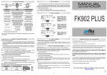
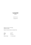
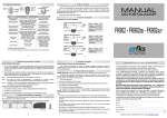
Spreadsheets
There are two spreadsheets available for the
analysis of CICS performance data. The
Summary spreadsheet data is obtained from
the file created in the SMF110S file, and is
illustrated in Figure 1 on page 5. The following information is provided in the
SMF110S file for each hour:
DATE
Specifies the date CICS was executing.
The format can be mm/dd/yy or Lotus 1-23 date format (D1, D2, or D3).
TIME
Specifies the time of day.
CID
Specifies the CICS ID. The first four bytes
of the NETNAME are used.
#TASK
The number of transactions processed for
this period.
AVG RSP
The average response time for all transactions.
AVG WAIT
The average wait time for all transactions.
AVG CPU
The average CPU time for all transactions.
November 1, 1999
OSTOR
The average amount of storage used by all
transactions, in 1024 byte units.
AMC
The total number of access method calls
for all transactions.
I/O
The Total amount of I/O processing all
transactions performed. This includes
access method calls, journal puts,
synchpoints, BMS In, BMS Out, Temporary Storage AUX count, and Transient
Data get and put counts.
%CPU CICS
The total percentage of the CPU used by
the CICS region.
%CPU APPL
The percentage of the CPU used by the
application programs running within the
CICS region.
PAGE IN
The page in rate (pages per second) for the
CICS region.
PAGE OUT
The page out rate (pages per second) for
the CICS region.
COMPS
The number of storage bytes compressed
during the period.
PCP RSP
The average time for loading a program
during the period
PCP
The number of program loads during the
period.
PILOT/ CICS 3
KLM Technical Specialties, Inc. Exclusive Distributors: Axios Products, Inc.
DLI RSP
The average response time for a DLI call
(if DLI is installed).
DLI
The number of DLI calls during the period
(if DLI is installed).
DB2 RSP
The average response time for a DB2 call
(if DB2 is installed). This field is not
available in CMF. This field is provided
for compatibility with TMON 8.2.
DB2
The number of DB2 calls during the period
(only for the DB2 option). This field is
not available in CMF. This field is
provided for compatibility with TMON
8.2.
UDB RSP
The average response time for a User
Database. This field is not available in
CMF. This field is provided for compatibility with TMON 8.2.
UDB
The number of User Database calls during
the period. This field is not available in
CMF. This field is provided for compatibility with TMON 8.2.
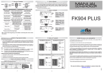
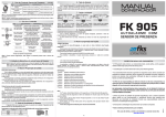
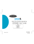
The Response spreadsheet data is obtained
from the file created in the SMF110R file,
and is illustrated in Figure 2 on page 7. The
following information is provided in the
SMFPC110R file for each transaction processed:
DATE
Specifies the date the transaction was
initiated by CICS. The format can be
mm/dd/yy or Lotus 1-2-3 date format (D1,
D2, or D3).
TIME
Specifies the time of day the transaction
was initiated by CICS in hhmm format.
TRAN
The transaction name.
T
Transaction types as follows:
A Auto initiated transaction.
P Printer transaction.
T Terminal initiated transaction.
Z Conversational transaction.
#TASK
The number of transactions processed for
this period.
95% RSP
The 95th percentile of the transaction
response time for this transaction code.
This means that the value reported is
higher than 95 percent of the transactions
processed for this period.
75% RSP
The 75th percentile of the transaction
response time for this transaction code.
50% RSP
The 50th percentile of the transaction
response time for this transaction code.
25% RSP
The 25th percentile of the transaction
response time for this transaction code.
MIN RSP
4 PILOT User's Guide
November 1, 1999
KLM Technical Specialties, Inc. Exclusive Distributors: Axios Products, Inc.
The minimum transaction response time
for this transaction code.
November 1, 1999
Specifies the CICS ID. The first four bytes
of the NETNAME are used.
MAX RSP
The maximum transaction response time
for this transaction code.
95% WT
The file control wait time of the 95th
percentile value as described above.
50% WT
The file control wait time of the 50th
percentile value as described above.
MIN WT
The minimum file control wait time for
this transaction code.
MAX WT
The maximum file control wait time for
this transaction code.
CPU
The average amount of CPU time used by
the transaction.
STOR
The average amount of storage the transaction used, in 1024 byte units.
AVG I/O
The average amount of I/O processing the
transaction performed. This includes
access method calls, journal puts,
synchpoints, BMS In, BMS Out, Temporary Storage AUX count, and Transient
Data get and put counts.
PAGEIN
The average number of page faults for this
transaction.
CID
PILOT/ CICS 5
KLM Technical Specialties, Inc. Exclusive Distributors: Axios Products, Inc.
November 1, 1999
A1: [W9]
MENU
IMPORT GRAPHS PRINT RETURN SAVE SETUP EXIT
Load a ".PRN" file for a CICS Summary Report
A
B
C
D
E
F
G
H
I
J
1
Spreadsheet
Version
2
SUMCICS
V1L5.0
3
4
PILOT/CICS Summary Template
5
6
7
AXIOS PRODUCTS, INC. PILOT/CICS (C) 1993 TMV8 KLM Technical
Specialti
8
CICS REGIONS:TS04
9
DATE
TIME CID #TASKS
AVG_RSP AVG_WAIT AVG_CPU OSTOR DSA
AMC
10 07/14/93 1900 TS04
129
0.089
0.038
0.0124
678 11268
267
11 07/14/93 2000 TS04
184
0.055
0.022
0.0055
678 11268
109
12 07/14/93 2100 TS04
300
0.093
0.023
0.0092
678 11268
1334
13 07/14/93 2200 TS04
403
1.295
1.058
0.9881
678 11268
9514
14 07/14/93 2300 TS04
192
0.253
0.143
0.1019
678 11268
1994
15 07/15/93
0 TS04
218
55.875
0.746
0.0192
616 4952
277
16 07/15/93 100 TS04
183
0.177
0.065
0.0173
616 6744
850
17 07/15/93 200 TS04
737
0.201
0.064
0.0488
616 7404
5344
18 07/15/93 300 TS04
1925
0.136
0.017
0.0151
616 7536
12343
19 07/15/93 400 TS04
284
0.971
0.746
0.6741
616 9180
5208
20 07/15/93 500 TS04
339
0.801
0.606
0.5528
676 9180
6190
23-Nov-93 03:18 PM
CMD
Figure 1 Summary Template for CMF
6 PILOT User's Guide
KLM Technical Specialties, Inc. Exclusive Distributors: Axios Products, Inc.
November 1, 1999
A1:
MENU
IMPORT GRAPHS PRINT RETURN SAVE SETUP EXIT
Load a ".PRN" file for a CICS Response Time Report
A
B
C
D
E
F
G
H
I
1
Spreadsheet
Version
2
RSPCICS
V1L5.0
3
4
5
6
CICS Response Time Template
7
8
PILOT/CICS (C) 1986-1993
9
Notes:
10
There are macros you can use to return to the menus.
11
Press:
12
ALT-A to bring up the query menu
13
ALT-G to bring up the graphs menu
14
ALT-M to bring up the main menu (this screen)
15
ALT-P to bring up the print menu
16
(Use CTRL in the Windows version of Lotus)
17
18
19
20
23-Nov-93 03:20 PM
CMD
Figure 2 Response Template for CMF
PILOT/ CICS 7
KLM Technical Specialties, Inc. Exclusive Distributors: Axios Products, Inc.
8 PILOT User's Guide
November 1, 1999
KLM Technical Specialties, Inc. Exclusive Distributors: Axios Products, Inc.
November 1, 1999
PILOT/CICS for The Monitor™
Introduction
SMFLOG
PILOT/CICS allows users to format The
Monitor™ detail records for capacity planning
and performance tuning on the system and
transaction level. Two versions of the
program are provided.
The program
MONPCLMK executes as a stand-alone
program to process the records created by
The Monitor™ Version 8. The program
SMFPCLMK executes as a stand-alone program to process
records created by
Landmark's database utility program
$DBUTIL, and supports all earlier versions
of The Monitor™. Both programs read The
Monitor's™ detail and system interval records.
MONPCLMK and SMFPCLMK have two
input files:
LMKIN
Specifies the input file that contains The
Monitor™ records. SMFIN data files are
not processed when this DD statement is
included.
SMFCTL
Specifies a control card file to indicate the
regions and transactions to be processed.
If this file is omitted, all regions and
transactions are processed.
MONPCLMK and SMFPCLMK have at least
two output files:
PILOT/ CICS 9
KLM Technical Specialties, Inc. Exclusive Distributors: Axios Products, Inc.
This file is always required. This file
provides information on the data processed.
SMFMONS
This optional file provides summary information for each region processed. When
this DD stastement is omitted, a file for
downloading is not created.
SMFMONSR
This optional file provides summary information for each transaction processed.
When this DD statement is omitted, a file
for downloading is not created.
Do not run these programs as user exits of
READSMF when processing non-SMF
data.
Control Cards and Parameters
There is one keyword with three operands
that may be specified in the SIMCTL file.
The REGION keyword must start between
columns 2 and 71 and be followed by a
blank. Operands for these control cards must
be separated by a comma. The REGION
control card is needed to reduce output.
The format of the control card follows.
REGION
INCL=(t1,t2,t3,…),
IREG=(r1,r2,r3..),
EREG=(r1,r2,r3..),
The statement may be continued on the next
card. No special continuation character is
required.
10 PILOT User's Guide
November 1, 1999
KLM Technical Specialties, Inc. Exclusive Distributors: Axios Products, Inc.
Example:
1
2
3
4
123456789012345678901234568901234568
9012345
November 1, 1999
Parameters on the JCL EXEC
Card
REGION EXCLUDE=(CSSN,TRAN05) NO
STATS
GDATE
Specifies that the date be printed in
mm/dd/yy format instead of Lotus 1-2-3
(D1) format.
EXCL=(TRN1,TRN2,TRN3,TRN4,....)
Where “TRNx” represents a transaction
code to be excluded from processing.
An “*” may be used as a mask in the
last three positions. Up to 50 transactions may be specified.
COMREGS
Specifies that all input data found is to be
processed as one output file combining all
regions found.
INCL=(TRN1,TRN2,TRN3,TRN4,....)
Where “TRNx” represents a transaction
code. Specifies a group of transactions
that are to be included for processing.
An “*” can be used as a mask in the last
three positions. Up to 50 transactions
may be specified.
The EXCL and INCL keywords can be
specified using an “*” as a mask for transaction names.
For example, INCL=
(TR*,TI*) will include all transactions that
start with TR or TI only.
IREG=(CID1,CID2,CID3,CID4,....)
Specifies a group of CICS regions to be
included for processing. Up to 50 CICS
IDs maybe specified.
EREG=(CID1,CID2,CID3,CID4,....)
Specifies a group of CICS regions to be
excluded from processing. Up to 50
CICS IDs maybe specified.
SEPREGS
Specifies that data is divided by regions
found on the input file.
JCL
PILOT/CICS for The Monitor™ is a standalone program:
//PCFMT EXEC
PGM=SMFPCLMK,
REGION=1720K
or
//PCFMT EXEC
PGM=MONPCLMK,
REGION=1720K
//STEPLIB
DD
DSN=TSU01.MYLIB
,DISP=SHR
//LMKIN DD DSN=BACKUP.LANDMAR
K.DATA.G0001V00,
//
UNIT=TAPE,
//
VOL=SER=123456,DISP=O
LD
//SMFLOG DD
SYSOUT=A
//SMFMONS DD
DSN=TSU01.CICSS
UM.PRN,
//
DISP=(,CATLG),
//
SPACE=(TRK,(4,4),RLSE)
//SMFMONSR
DD
DSN=TSU01.
CICSRSP.PR
N,
PILOT/ CICS 11
KLM Technical Specialties, Inc. Exclusive Distributors: Axios Products, Inc.
//
DISP=(,CATLG),
//
SPACE=(TRK,(4,4),RLSE)
//SMFCTL
DD
*
*
* COLLECT CICS TRANS. EXCEPT
SIGNON, SIGNOFF TRANS.
*
R E G I O N
EXCL=(CSSN,CSSF),IREG=(PRD1)
/*
Notes:
November 1, 1999
Specifies the date CICS was executing.
The format can be mm/dd/yy or Lotus 12-3 date format (D1, D2, or D3).
TIME
Specifies the time of day in hhmm format.
CID
CICS system identifier specified in
DFHSIT (1.7), DFHTCT (2.1)
SYSIDNT parameter.
1. STEPLIB
Used if SMFPCLMK is not in the link
list.
2. LMKIN
The input data set, containing TMON records.
3. SMFLOG
Statistics on the run.
4. SORTIN
Used as a workfile to calculate percentiles.
5. SMFMONS
CICS summary file to transfer to a PC.
6. SMFMONSR
The CICS summary response time file to
transfer to a PC.
7. SMFCTL
Control card data set.
#TASK
The number of transactions processed for
this period.
Spreadsheets
AMC
The total number of access method calls
for all transactions.
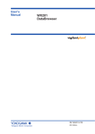
There are two spreadsheets available for the
analysis of CICS performance data. The
Summary spreadsheet data is obtained from
the file created in the SMFMONS file, and is
illustrated in Figure 3 on page 14. The
following information is provided in the
SMFMONS file for each hour:
DATE
12 PILOT User's Guide
AVG RSP
The average response time for all transactions.
AVG WAIT
The average wait time for all transactions.
AVG CPU
The average CPU time for all transactions.
STOR
The amount of operating system storage
available (OSCOR) in 1024 byte units.
I/O
The total amount of I/O processing all
transactions performed. This includes
access method calls, journal puts,
synchpoints, BMS In, BMS Out, Temporary Storage AUX count, and Transient
data get and put counts.
KLM Technical Specialties, Inc. Exclusive Distributors: Axios Products, Inc.
%CPU CICS
The total percentage of the CPU used by
the CICS region. Sum of TCB and SRB
CPU time. TMON collection option
“REALCPU” must be set to “Y”.
%CPU APPL
The percentage of the CPU used by the
application programs running within the
CICS region. TMON collection option
“REALCPU” must be set to “Y”
November 1, 1999
DB2_RSP
The average response time for a DB2 call
(if DB2 is installed).
DB2
The number of DB2 calls during the
period (if DB2 is installed).
UDB_RSP
The average response time for a user
database (IDMS, ADABASE, etc.) call.
PAG IN
The page in rate (pages per second) for
the CICS region.
UDB
The number of user database (IDMS,
ADABASE, etc.) calls during the period.
PAG OUT
The page out rate (pages per second) for
the CICS region.
INTVL
The number of seconds in the period.
COMPS
The number of program subpool compressions during the period.
The Response spreadsheet data is obtained
from the file created in the SMFMONSR file,
and is illustrated in Figure 4 on page 14.
The following information is provided in the
SMFMONSR file for each transaction
processed:
PCP_RSP
The average time for loading a program
during the period.
PCP
The number of program loads during the
period.
DSA_HWM
The highest amount of storage allocated
from dynamic storage area during the
period. In 1024 byte units.
DLI_RSP
The average response time for a DLI call
(if DLI is installed).
DATE
Specifies the date the transaction was
initiated by CICS. The format can be
mm/dd/yy or Lotus 1-2-3 date format
(D1, D2, or D3).
TIME
Specifies the time of day the transaction
was initiated by CICS, in hhmm format.
TRAN
The transaction name.
T
DLI
The number of DLI calls during the
period (if DLI is installed).
Transaction types as follows:
A Auto initiated transaction.
P Printer transaction.
PILOT/ CICS 13
KLM Technical Specialties, Inc. Exclusive Distributors: Axios Products, Inc.
T
Z
R
I
Terminal initiated transaction.
Conversational transaction.
Inter-region transaction.
Inter-system transaction.
#TASK
The number of transactions processed for
this period.
95% RSP
The 95th percentile of the transaction
response time for this transaction code.
This means the value reported is higher
than 95 percent of the transactions processed for this period.
75% RSP
The 75th percentile of the transaction
response time for this transaction code.
November 1, 1999
MIN WT
The minimum file control wait time for
this transaction code.
MAX WT
The maximum file control wait time for
this transaction code.
CPU
The average amount of CPU time the
transaction used.
STOR
The average amount of storage the transaction used in 1024 byte units.
50% RSP
The 50th percentile of the transaction
response time for this transaction code.
AVG I/O
The average amount of I/O processing
the transaction performed. This includes
access method calls, journal puts,
synchpoints, BMS In, BMS Out, Temporary Storage AUX count, and Transient
Data get and put counts.
25% RSP
The 25th percentile of the transaction
response time for this transaction code.
DLI_RSP
The average response time for a DLI call
(if DLI is installed).
MIN RSP
The minimum transaction response time
for this transaction code.
DLI
The number of DLI calls during the
period (if DLI is installed).
MAX RSP
The maximum transaction response time
for this transcation code.
DB2_RSP
The average response time for a DB2 call
(if DB2 is installed).
95% WT
The file control wait time of the 95th
percentile value as described above.
DB2
The number of DB2 calls during the
period (if DB2 is installed).
50% WT
The file control wait time of the 50th
percentile value as described above.
UDB_RSP
The average response time for a user
database (IDMS, ADABASE, etc.) call.
14 PILOT User's Guide
KLM Technical Specialties, Inc. Exclusive Distributors: Axios Products, Inc.
November 1, 1999
UDB
The number of user database (IDMS,
ADABASE, etc.) calls during the period.
PGIN
The average number of page faults for
this transaction.
PGOUT
The average number of page outs for this
transaction.
CID
CICS system identifier specified in
the DFHSIT (1.7) or DFHTCT (2.1)
SYSIDNT parameter.
PILOT/ CICS 15
KLM Technical Specialties, Inc. Exclusive Distributors: Axios Products, Inc.
November 1, 1999
A1: [W9]
MENU
IMPORT GRAPHS PRINT RETURN SAVE SETUP EXIT
Load a ".PRN" file for a CICS Summary Report
A
B
C
D
E
F
G
H
I
J
1
Spreadsheet
Version
2
SUMCICS
V1L5.0
3
4
PILOT/CICS Summary Template
5
6
7
AXIOS PRODUCTS, INC. PILOT/CICS (C) 1993 TMV8 KLM Technical
Specialti
8
CICS REGIONS:TS04
9
DATE
TIME CID #TASKS
AVG_RSP AVG_WAIT AVG_CPU OSTOR DSA
AMC
10 07/14/93 1900 TS04
129
0.089
0.038
0.0124
678 11268
267
11 07/14/93 2000 TS04
184
0.055
0.022
0.0055
678 11268
109
12 07/14/93 2100 TS04
300
0.093
0.023
0.0092
678 11268
1334
13 07/14/93 2200 TS04
403
1.295
1.058
0.9881
678 11268
9514
14 07/14/93 2300 TS04
192
0.253
0.143
0.1019
678 11268
1994
15 07/15/93
0 TS04
218
55.875
0.746
0.0192
616 4952
277
16 07/15/93 100 TS04
183
0.177
0.065
0.0173
616 6744
850
17 07/15/93 200 TS04
737
0.201
0.064
0.0488
616 7404
5344
18 07/15/93 300 TS04
1925
0.136
0.017
0.0151
616 7536
12343
19 07/15/93 400 TS04
284
0.971
0.746
0.6741
616 9180
5208
20 07/15/93 500 TS04
339
0.801
0.606
0.5528
676 9180
6190
23-Nov-93 03:18 PM
CMD
Figure 3 Summary Template for The Monitor™
16 PILOT User's Guide
KLM Technical Specialties, Inc. Exclusive Distributors: Axios Products, Inc.
November 1, 1999
A1:
MENU
IMPORT GRAPHS PRINT RETURN SAVE SETUP EXIT
Load a ".PRN" file for a CICS Response Time Report
A
B
C
D
E
F
G
H
I
1
Spreadsheet
Version
2
RSPCICS
V1L5.0
3
4
5
6
CICS Response Time Template
7
8
PILOT/CICS (C) 1986-1993
9
Notes:
10
There are macros you can use to return to the menus.
11
Press:
12
ALT-A to bring up the query menu
13
ALT-G to bring up the graphs menu
14
ALT-M to bring up the main menu (this screen)
15
ALT-P to bring up the print menu
16
(Use CTRL in the Windows version of Lotus)
17
18
19
20
23-Nov-93 03:20 PM
CMD
Figure 4 Response Template for The Monitor™
PILOT/ CICS 17
KLM Technical Specialties, Inc. Exclusive Distributors: Axios Products, Inc.
18 PILOT User's Guide
November 1, 1999
KLM Technical Specialties, Inc. Exclusive Distributors: Axios Products, Inc.
November 1, 1999
Modeling
Introduction to Modeling
PILOT/CICS provides two models. The
first, MODLCICS, is an analytic queuing
model to calculate average response times
based upon 9 input parameters. The second,
SIMCICS, is a model used to simulate a
multi-tasking operating system by defining
transaction/request-oriented workloads.
MODLCICS executes under Lotus 1-2-3 and
can be used to model simple CICS environments. More complex environments require
more knowledge about the expected results
and the input factors can be difficult to
estimate.
SIMCICS has two components, a mainframe
model generator, and the actual simulator
that executes on the PC. The simulator can
model more complex environments.
MODLCICS Spreadsheet
The spreadsheet MODLCICS provides an
automated tool for capacity planning and
performance analysis of the CICS environment. This program is an analytic queuing
model which calculates average CICS response times based on 9 input parameters.
These parameters represent average utilization factors affecting memory, the DASD
subsystem, and CPU use. The model was
originally introduced in an article appearing
in the December, 1982 issue of the IBM
Systems Journal.
The value of using an analytic queuing model
for capacity planning is twofold:
! First, an analytic model consists of
equations which yield a single result
(i.e., response time) when executed.
Analytic models can be run over and
over with a minimal use of CPU cycles. This is very important when
you are examining many alternatives
and playing the what/if game; and
! Second, a queuing model produces a
non-linear result of response time
versus resource utilization. This is,
in fact, how real on-line systems behave. Models based on linear approximations are generally only
accurate for a narrow range of resource utilization.
MODLCICS provides 5 user options. A list
of these options is displayed when the user
menu is invoked. This is done by pressing
the Alt and M keys at the same time. Together, these options provide the tools for
automating a capacity planning methodology
for CICS.
Model Parameters
The nine input parameters
MODLCICS spreadsheet are:
for
the
CPUR
The average CPU service time for CICS
transactions. This value is expressed in
PILOT/ CICS 19
KLM Technical Specialties, Inc. Exclusive Distributors: Axios Products, Inc.
seconds and can be calculated by
dividing the total CPU seconds used
by CICS by the total number of
completed transactions.
These
measurements should be made for a
reasonable period of time (1 hour is
recommended).
This value is
obtained from the PILOT/CICS
summary spreadsheet.
TP
The average service time for the paging
packs. Also expressed as seconds, this
value is obtained from the PILOT/MVS
Page data set spreadsheet or can be read
from an RMF disk subsystem report.
Since there will probably be more than
one page pack defined, this value should
represent a composite of all the active
page packs.
UP
The average utilization of the paging
packs. This value represents the fraction
of time the pack is busy (i.e., .30 for a
pack which averages 30% busy.)
TD
The average service time for the data
base packs. Similar to TP above, this
value represents a composite service time
for all the packs used by CICS for data
base disk I/O. This data can be obtained
from the PILOT/MVS DASD
spreadsheet, which can selectively choose
packs.
UD
The average utilization of the data base
packs. Similar to UP above.
IOR
The average I/O rate for CICS transactions. This value represents the number
20 PILOT User's Guide
November 1, 1999
of real disk I/Os executed on behalf of a
CICS transaction. This value can be
calculated by dividing the total number of
disk I/Os issued by CICS to the data base
packs by the total number of completed
transactions.
UH
The average utilization of the CPU by
tasks which run at a higher dispatching
priority than CICS. Expressed as a
fraction, this value measures the CPU
capacity which is not available to CICS.
Tasks running at a higher priority than
CICS are typically VTAM, JES, and the
operating system. Unique installation
conditions may require that another subsystem (e.g., IMS) run at a higher priority than CICS. This value can be estimated by examining the PILOT/MVS
workload activity reports or RMF. Tasks
which run at a higher priority than CICS
can be identified by their performance
group number. The RMF reported CPU
service times can be converted to CPU
seconds by using the appropriate
conversion factor. Dividing the CPU
seconds used by the elapsed time yields
the utilization by higher priority tasks. In
addition, the utilization of the operating
system which has not been included in a
reported performance group must be
added to this number. This can be estimated by comparing the total CPU
utilization reported by RMF with the total
number of CPU seconds reported for all
performance groups. The difference
between the total utilization and the total
reported utilization for all performance
groups is the unreported utilization
charged to system overhead.
PFR
KLM Technical Specialties, Inc. Exclusive Distributors: Axios Products, Inc.
The average page fault rate for the CICS
task. Expressed as page faults per second, this number represents the number
of times each second that CICS must stop
to wait for a page fault to be resolved.
This value can be obtained from the
PILOT/CICS summary spreadsheet.
XR
The average CICS transaction rate expressed as transactions per second. This
value is obtained from the PILOT/CICS
summary spreadsheet or it can be calculated by dividing total number of CICS
completed transactions by the elapsed
time.
The input parameters can be produced by the
model generator program SIMBUILD.
Depending on the options selected, the user
may change one or more of the 9 parameters
to alter the model. Some of the options will
allow the user to select a starting CICS
transaction rate (XR) and a delta transaction
rate (DXR). This will allow the model to
vary the transaction rate evenly, beginning
with XR and incrementing by DXR to provide a smooth curve.
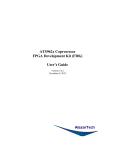
Spreadsheet Features
Options
November 1, 1999
A sample of the template’s main panel can be
seen in Figure 5 on page 29.
The 5 options are:
RESPONSE
Calculates the average CICS response
times for a range of CICS transaction
rates. A sample of the template’s Response panel and menu can be seen in
Figure 6 on page 29.
SLOPE
Calculates the slope of response time
versus transaction rate for a range of
transaction rates. These values can be
used to estimate the breaking point (out
of capacity condition) of the response
time/transaction rate curve. A sample of
the template’s Response/Slope panel and
menu can be seen in Figure 6 on page
29.
FACTORS
Calculates sensitivity factors for each
model input parameter. The sensitivity
factor for each parameter represents the
percent change in response time caused
by a 1 percent increase in the input
parameter. For example, a sensitivity
factor of 5 for page fault rate (PFR)
means that a 1 percent increase in page
fault rate will cause a 5 percent increase
in response time. A sample of the template’s Factors panel and menu can be
seen in Figure 7 on page 30.
The MODLCICS spreadsheet includes 5 user
options. A list of these options can be
displayed by pressing the
and
keys at
BEST/WORST
the same time. Please note that the Lotus 1Calculates a best/worst case capacity plan
2-3 Calc (
) key must be used when the
based on a 12 month projection of
values are changed. If the Calc indicator is
transaction rates. Best/worst case condidisplayed on the bottom line of the display,
tions are expressed as 2 sets of model
then the spreadsheet needs to be recalculated.
parameters. Transaction rates are proPress Calc to do this. If you are in a menu,
jected over 12 months and the model
first press
to get to a READY prompt.
PILOT/ CICS 21
KLM Technical Specialties, Inc. Exclusive Distributors: Axios Products, Inc.
calculates both best and worse case
response times. You can also enter a
maximum allowable response time
value. This value will be graphed
along with the best/worse case
response times to show where the
capacity of the CICS system is
exceeded. A sample of the template’s
Best/Worst Case panel and menu can
be seen in Figure 8 on page 30.
Additional information on the use of this
option can be found in methodology discussion on page 22.
OPTIONS
Calculates 1 to 4 sets of response times
for a range of transaction rates. Each set
of response times is derived from a
different set of model parameters. Up to
4 configurations may be specified. The
graphs of response times versus transaction rates can be used to judge the relative improvement in one option over
another. Each option is expressed as a
set of model input parameters. Once
again, a maximum allowable response
time can be input to show the capacity
limits of each option. A sample of the
template’s Options panel and menu can
be seen in Figure 9 on page 31.
Each option can be selected from the command menu using the first letter of the option
(i.e., F for FACTORS), or by pressing the
cursor keys to highlight the option and then
pressing the
key. A description of each
highlighted option will appear on the second
line. When an option is selected, a sub-menu
will appear. All of the sub-menus are the
same. They provide 2 user options. These
are: CHANGE and GRAPH.
22 PILOT User's Guide
November 1, 1999
CHANGE
Alter one or more of the input parameters
for the currently selected option. Lotus
1-2-3 will automatically position the
cursor at the first model input parameter
for this option. This will typically be the
CPUR value. At the same time, the user
menu will be erased from the command
line. This means the full facilities of
Lotus 1-2-3 are available to change the
input parameters. To display the menu
again you must press
.
The spreadsheet has been initially set
with the protection switch enabled. This
means that only the fields marked as
unprotected can be changed. These fields
will show up as high intensity on a
monochrome display and as white on a
color display. Attempting to change a
protected field will produce a beep as an
error indication. The auto-recalculation
switch has been set off, so be sure to
press the
(Recalculate or Calc) key
after all changes. This will recalculate all
the dependent cells. Above each set of
input cells is an unprotected cell called
TITLE which will appear as a title of the
graph created for this option.
GRAPH
Produces a graph of the results calculated
by CHANGES. These graphs will differ
depending on the option chosen. The
GRAPH option requires a graphic display
and adapter. See the Lotus 1-2-3 manual
for a description of the supported
displays. To save the graph for a printer
or plotter output, type:
save) and give it a name as described in
the Lotus 1-2-3 manual. Once a graph
has been selected it can be displayed
again by simply pressing the
(GRAPH) key. If a model parameter is
(graph
KLM Technical Specialties, Inc. Exclusive Distributors: Axios Products, Inc.
changed, first press
to recalculate
and then press
to graph. The new
results will be displayed.
November 1, 1999
spreadsheet. This data can be viewed by
pressing the
(GOTO) key, then SF
and then
. To return to the input
area, press the
key.
This section describes how to use the options
provided in the MODLCICS spreadsheet.
! To display a graph of response time
versus transaction rate, press
then
press
to select the Response option,
then press
to select Graph.
Using the Response option:
Using the Slope and Factors Options
! Invoke the user menu by pressing the
keys.
! If you select either SLOPE or FACTORS
and then the CHANGE option, you will
be positioned over the same input area
used by the RESPONSE option. These
three options use the same set of model
input values.
Using the Spreadsheet
! Press
to select the Response option.
! Press
to select the Change option.
! Change one or more model input parameters. The XR value is the starting
transaction rate. The DXR value will be
used to increment the transaction rate.
! Change the cell to the right of the label
TITLE to describe this modeling run. It
will appear as a title in the graph.
! Press the
key to recalculate the dependent cells. This causes several model
values to be recalculated. First, the
transaction rate column is recalculated,
starting with the XR value and incremented by DXR. Next, the response
time values are recalculated based on the
selected model input parameters and the
calculated transaction rates. To the right
of the response time column is the slope
of response time versus transaction rate.
These cells are also recalculated. Finally, the sensitivity factors for each model
input parameter are recalculated. These
values are stored in a different part of the
! Selecting GRAPH for the SLOPE option
will display a graph of both response time
and slope of response time versus
transaction rate. This provides a visual
perspective of how transaction rate
affects response time and where the knee
of the curve appears. For example, a
value of slope equal to 2 means that the
average CICS response time is increasing
twice as fast as transaction rate. A rule
of thumb is to call this point the knee of
the curve.
See the methodology discussion on page
22 for additional advice on how to use
this data.
! The values for slope are displayed in a
column to the right of the response times.
The sensitivity factor values are displayed
in a different part of the spreadsheet, as
described above.
PILOT/ CICS 23
KLM Technical Specialties, Inc. Exclusive Distributors: Axios Products, Inc.
Using Best/Worst and Options
! Selecting BEST/WORST or OPTIONS
and then CHANGE will position the
cursor over the input values for these
options.
BEST/WORST case input
values consist of two sets of model input
parameters. Any of the model parameters can be changed to indicate a best and
worst case set of conditions. Values can
also be selected for transaction rates
corresponding to twelve month's growth.
! Pressing
will recalculate the response
times for each of the twelve months for
both best and worst case values.
! By changing the value for MAX RSP
(maximum acceptable response time) the
capacity limitations can be forecasted.
Displaying a graph of BEST/WORST
will show the average response time for
both best and worst case values plotted
along with MAX RSP. The intersection
of the BEST/WORST lines with the
MAX RSP line represents the month
when CICS capacity for each option is
exceeded.
! The input area for OPTIONS is similar to
BEST/WORST but includes four sets of
input values. These correspond to the
four options that can be modeled (i.e.,
different CPU, more memory, etc.). The
values for transaction rate are calculated
from a starting value of XR and incremented by DXR.
! Displaying a graph of OPTIONS shows
the curves of response time versus transaction rate for each of the four options.
The intersection of each curve with MAX
RSP can be defined as the capacity limit
for that option. The value of transaction
24 PILOT User's Guide
November 1, 1999
rate at the point of intersection can be
defined as the maximum load that option
can sustain with acceptable performance.
Methodology
This section describes a step-by-step methodology which can be used to create a capacity plan for CICS. The steps that follow
use the capabilities provided in the five user
options which make up the MODLCICS
spreadsheet.
Calibrating the Model
Calibrating the model means testing the
model's ability to predict the current environment. This is done by tracking model
input parameters using one or more tools
(i.e., PILOT/CICS, PILOT/MVS, CICS
PARS and RMF) and using the RESPONSE
option to compare predicted response times
against measured values. Measurements
should be made for a peak hour of CICS use
and should include at least five days of data.
This will ensure that you are not measuring
an unusual day or spike condition. If the
CICS system makes use of conversational
mode transactions, then the tracking tool
must report transactions and response time
accordingly. This means that a long conversational mode transaction must be reported as
several shorter transactions. These values
should represent internal response time and
should not include think time or terminal
network delay.
If the model's predicted response time falls
within 20% of measured response time, the
model can be considered calibrated. An
error greater than 20% can be caused by
several factors. First, ensure that the input
KLM Technical Specialties, Inc. Exclusive Distributors: Axios Products, Inc.
parameters and CICS response time were
measured correctly. A misplaced decimal
point or wrong use of units (i.e., transactions
per minute not per second) will certainly
invalidate the model.
Another cause may be an internal bottleneck
within CICS. Internal bottlenecks represent
conditions which degrade CICS performance
despite the availability of CPU cycles,
memory, and DASD resources. Some
examples are improperly set values of
MAXTASK, VSAM buffers, and
IMS/DATABASE strings. These represent
artificial constraints to performance and
cannot be accounted for in the model. In a
sense, these bottlenecks represent tuning
problems and must be separated from capacity planning issues.
Calculate the Maximum Acceptable Response Time
Before creating a capacity plan one must
define and quantify “capacity exceeded.”
This can be done by calculating the maximum acceptable response time for your
installation. A good rule of thumb is to
locate the knee of the curve of response time
versus transaction rate. If the previous rule
of thumb is used, this occurs where the slope
of response time equals 2. As noted earlier,
this represents that point on the response
time/transaction rate curve where response
time is growing twice as fast as transaction
rate. Since this is an exponential curve, the
expected response times become unstable
from this point forward. Use the SLOPE
option to calculate response times and slope
of response time for varying transaction
rates. The response time value which
corresponds to a slope of 2 is the value to
look for. In plain language, this value
November 1, 1999
represents the maximum acceptable response
time for your installation. This value is
installation dependent. If the base values of
the model input parameters are changed, the
value of response time which corresponds to
a slope of 2 will also change.
Create a Capacity Plan Based On Expected Transaction Rate Growth
A capacity plan can be created which will
identify the capacity limits of your current
installation. This is done by projecting
transaction rate growth over a twelve month
interval. Start with a base value for the
transaction rate (equal to the average measured XR for the peak hours of CICS activity). Project the transaction rate growth based
on your installation’s plans. These plans
should include the following:
! New CICS applications;
! Growth in the use of existing applications
due to new users; and
! Growth in the use of existing applications
due to increased activity by existing
users.
If CICS usage data has been tracked, this
data can be used to help in your projections.
Use the BEST/WORST option to calculate
CICS response times for the twelve months
of projected transaction rates. Model input
parameters for best case should be set to the
base values currently measured in your
installation. Worst case values should be set
to reflect possible growth in one or more
model parameters over the next twelve
months. For example, if the page fault rate
varies from 2 to 4 pages per second on a
daily basis, use the following technique. Set
PILOT/ CICS 25
KLM Technical Specialties, Inc. Exclusive Distributors: Axios Products, Inc.
the best case value of page fault rate (PFR) to
2 and set the worst case value to 4. This
assumes that over time the average PFR may
grow from 2 to 4 pages per second. This
approach can be used with other model
parameters as well. Be sure to input the
maximum acceptable response time (MAX
RSP) calculated in step 2. When a graph of
BEST/WORST is displayed, the response
times are plotted over the twelve month
period for both best and worst case input.
The intersection of maximum acceptable response time and these two lines represents
the point where your installation's capacity is
exceeded. The time of year corresponding to
these two points can be defined as the best
case and worst case limits of CICS capacity.
Another way to define these times is to
expect response time to begin to degrade at
the worst case limit and to certainly become
unacceptable at the best case limit. If a
twelve month projection fails to exceed your
capacity limit, then double the interval by
treating each monthly value as a two month
step.
Identify Performance Bottlenecks
Once the capacity limits for the installation
have been defined, different configuration
changes can be put into the model to fix the
problem (increase the limits). These changes
are generally limited to increasing one or
more computer resources. These include:
adding real memory; upgrading the DASD
sub-system; and installing a faster CPU.
Before selecting changes, try to determine
the primary bottleneck affecting response
time. This can be done by using the Factors
option to calculate sensitivity factors. Select
the Factors option and select the Change
sub-option from the user menu. The input
parameters should be entered to reflect the
model input values at the point of unaccept-
26 PILOT User's Guide
November 1, 1999
able performance. These values can be taken
from the point where either best case or
worst case projections cross the maximum
acceptable response time line. Press
to
recalculate the sensitivity factors for each
model input parameter. These values can be
viewed by selecting the GRAPH option or
can displayed by pressing
(GOTO), type
SF, then press enter. The sensitivity factors
(SF) represent the percent increase in response time caused by a 1 percent increase in
each input parameter. The higher the
sensitivity factor, the more sensitive is
response time to that input parameter. These
values can be used to identify which
computer resource is the dominant cause of
poor performance. For example, a high
value for the page fault rate SF would indicate a real memory constraint. High SF
values for disk service times and disk utilization parameters (TD and UD) would
indicate a problem with the DASD subsystem. And a high value of SF for CPU
service time (CPUR) would certainly indicate
that response time is sensitive to the speed of
the CPU. You can use the model to examine
the effects of relieving these bottlenecks.
For example, if a real memory constraint is
indicated, reduce the page fault rate (PFR)
parameter in the input field and calculate the
new response time. A sharp reduction in
response time will verify the bottleneck
caused by excessive paging.
Compare Configurations to Solve Capacity Problems
Based on the calculation of sensitivity factors, resources affecting performance can be
determined and consequently a solution may
be found to the problem. It is possible to
examine configuration changes to extend
CICS capacity. Selecting Options allows you
KLM Technical Specialties, Inc. Exclusive Distributors: Axios Products, Inc.
to model up to four configuration changes at
the same time. The graph produced for this
option allows you to compare the relative
benefits of each option. The intersection of
maximum acceptable response time and each
response time/transaction rate curve indicates
the capacity limits for each option. The
transaction rate below each intersection is the
maximum CICS load supported by that
option. The percent increase in the transaction rate limit for option two over option one
represents the percent increase in capacity of
option two over option one. If you divide
this number by the cost of option two, you
have the percent increase in capacity per
dollar spent. Comparing these numbers will
show you the relative cost of each option.
Assuming more than one option meets your
objective for extending CICS capacity, the
most cost effective option can be chosen.
Choosing the Model Input Parameters
The value of the CICS model is its ability to
predict response time for a variety of configuration changes. But before the model can
be used, you must be able to translate these
changes into the input parameters understood
by the model. This section will offer advice
on how that is done.
Adding Real Memory
Adding real memory will affect CICS response time in proportion to the page fault
rate. In other words, if the page fault rate is
low (i.e., 1 to 2 pages per second) then the
effect of adding real memory will be
minimal. If the page fault rate is high, the
addition of real memory can have a major
impact on performance. Since you typically
November 1, 1999
add real memory in large blocks (4 or more
megabytes), one can assume that page fault
rates will be dramatically reduced. If the
current rate is 5 to 7 page faults per second,
adding 4 or more megabytes of memory will
initially reduce the page fault rate to 2 or
less.
Changing the DASD Subsystem
Changes to the DASD subsystem can be
modeled by changing the following model
input parameters: page pack service time and
utilization (TP & UP); and data base pack
service time and utilization (TD & UD).
DASD changes can include adding additional
disk control units, channels, disk packs, or
cache controllers. Choosing model input
values to model these changes will require
intelligent “guestimates” based on a good
understanding of the differences between the
current DASD subsystem and the proposed
changes.
As an example, assume the current subsystem
consists of 3350 disks and that you wish to
model the effects of converting to 3380s.
Also, assume the base value of TD, UD, TP,
and UP are .035, .40, .030, and .36
respectively. With the knowledge that
average seek times should improve from .025
to .015 seconds and the data transfer rates
improve from 1.2 to 3.0 megabytes per
second (3350 vs 3380), the estimated new
parameters are follows: TD (from .035 to
.020), UD (.40 to .25), TP (.030 to .018),
and UP (.36 to .20). These reductions are
estimates based on both a knowledge of the
current environment as well as an understanding of the proposed changes. In most
installations, the 4 DASD parameters will not
have a large impact on performance and
errors in these estimates will have a small
PILOT/ CICS 27
KLM Technical Specialties, Inc. Exclusive Distributors: Axios Products, Inc.
effect on calculated response time. If the
impact of a DASD change is uncertain,
assume a conservative decrease in these
parameters and examine the sensitivity
factors to measure their impact on response
time. If the sensitivity factors are low, then
the effect will be minimal.
Changing the CPU
Probably the most important change to an
installation's capacity will be an upgrade to a
faster CPU. Modeling the replacement of a
uni-processor with another uni-processor is
fairly straight forward. The parameters
affected by this kind of change will be CICS
CPU service rate (CPUR) and utilization of
the CPU by tasks running higher priority
than CICS (UH). Changes in these parameters should be scaled to the ratio of internal
speed of the 2 CPUs. These numbers are
published by IBM as tables of MIPS (Machine instructions per second). A ratio of 2
to 1 (new CPU MIPS to old CPU MIPS)
indicates the new CPU is twice as fast as the
old CPU. This means we can reduce the
base value of CPUR by a like factor. For
example, if the new CPU is 3 times faster
than the current CPU we can calculate the
new CPUR as old CPUR divided by 3.
The same logic can be applied to the UH
parameter, but in real life a faster CPU will
probably be executing more work. This
means the UH value will probably be reduced, but not as much as was CPUR. A
conservative approach would be to scale UH
by the ratio of MIPS and then add back in
10-20% of its new value. For example,
modeling UH on a CPU which is 3 times
faster than the current CPU can be done as
follows: assuming the current UH=.15, let
the new UH=.15/3 plus (20% of .05) =.06.
28 PILOT User's Guide
November 1, 1999
When modeling a new CPU which is a
multi-processor, a different approach is
taken. First, consider that CICS is a singletasking system. This means that CICS can
only execute on one processor at a time. The
value of CPUR must be computed as if the
speed of the new CPU is equal to the speed
of a single processor, not the combined speed
of all the processors.
High priority
utilization (UH), however, can be spread
over all the processors so we can divide this
value by the number of processors.
As an example, assume a base value of
CPUR=.24 and UH=.18. Assume an upgrade to a dyadic processor with an aggregate
MIPS equal to 4 times the current CPU.
Model this upgrade by again changing the
values of CPUR and UH. Assuming that the
memory size is not changing, the page fault
rate is ignored. Since CPUR is only affected
by the speed of one processor, set the new
CPUR = old CPUR/2 = .24/2 = .12. By
dividing the higher priority work over both
CPUs we can expect the CPU running CICS
to experience a UH equal to old UH/4 (half
as much work on a CPU which is twice as
fast). Once again to be conservative add
back 20 percent of the new number:
UH = .18/4 + .20(.18/4) = .054
If these numbers are put in the model it will
show CICS capacity is not dramatically
improved. This is caused by taking advantage of one half of the multi-processor. To
optimize CICS capacity on a multi-processor
you must run more than one copy of CICS.
A second copy of CICS can be modeled as if
it was running independent of the first copy
(one copy per processor with equal priority).
Assuming that CICS can be divided evenly,
you may run twice the maximum transaction
rate calculated for a single copy of CICS.
KLM Technical Specialties, Inc. Exclusive Distributors: Axios Products, Inc.
November 1, 1999
But this is probably an unrealistic
assumption. Dividing a production copy of
CICS into 2 equal parts is just not possible.
Even with the facilities of MRO (Multiple
Region Option) it is difficult to create 2 equal
parts from one CICS system. The effective
maximum transaction rate possible on a
dyadic processor will be something less than
twice the transaction rate calculated for a
single copy of CICS. The degree of
asymmetry between the 2 copies of CICS as
well as the overhead introduced by MRO will
tend to reduce the factor to a value less than
one half. If an upgrade to a multi-processor
(2 processors) is to be considered and if it is
expected to run 2 copies of CICS, calculating
the maximum transaction rate possible with
one copy of CICS is done by multiplying the
transaction rate by 2, and then reducing this
number by a factor of half the original
transaction rate. As an example, assume the
transaction rate on a single processor is 18
transactions per second. Assume an upgrade
to add a processor with the same MIP speed.
The maximum transaction rate possible is:
18*2 - 18/2 = 25 transactions per second.
Model Description
The following equations are used to calculate
the average CICS response time (RSP) as a
function of the 9 independent parameters in
the CICS analytic queuing model. These
parameters are described in Model
Parameters.
PILOT/ CICS 29
KLM Technical Specialties, Inc. Exclusive Distributors: Axios Products, Inc.
where:
30 PILOT User's Guide
November 1, 1999
KLM Technical Specialties, Inc. Exclusive Distributors: Axios Products, Inc.
November 1, 1999
A1: [W10]
MENU
RESPONSE FACTORS BEST/WORST OPTIONS MIPS RETURN SETUP EXIT
Calculate the slope of response times for varying transaction rates
A
B
C
D
E
F
G
H
I
1
Model Spreadsheet
Spreadsheet
Version
2
MODELCIC
V1L5.0
3
The following short-cuts are available:
4
ALT-M This Menu
ALT-B Best Case/Worst Case
5
ALT-R Response Time
ALT-O Option Comparison
6
ALT-F Sensitivity Factors ALT-C CPU MIPS Conversion
7
Use CTRL-x in the Windows version of Lotus.
8
9
Model Input Parameters:
10 CPUR - CPU Service Time
UP
- Page Busy
UH
- Super. Overhead
11 TP
- Page Service Time
UD
- Data Busy
PFR - Page Fault Rate
12 TD
- Data Service Time
IOR - I/O Rate
XR
- Arrival Rate
13
14
TITLE:
Current System
Delta of Arrival Rate
15
0.1
16
17
CPUR
TP
UP
TD
UD
IOR
UH
PFR
XR
18
0.100
0.035 0.150
0.035 0.300 5.000
0.200
2.2
6.0
19
6.1
20
6.2
23-Nov-93 03:30 PM
CMD
A1: [W10]
Figure
5 MODLCICS Template (Main Panel)
MENU
CHANGE RSP_XRATE SLOPE_XRATE SAVE_GRAPH PRINT RETURN
Change model input parameters for current system. Press CALC ALT-R for
menu.
A
B
C
D
E
F
G
H
I
1
Model Spreadsheet
Spreadsheet
Version
2
MODELCIC
V1L5.0
3
The following short-cuts are available:
4
ALT-M This Menu
ALT-B Best Case/Worst Case
5
ALT-R Response Time
ALT-O Option Comparison
6
ALT-F Sensitivity Factors ALT-C CPU MIPS Conversion
7
Use CTRL-x in the Windows version of Lotus.
8
9
Model Input Parameters:
10 CPUR - CPU Service Time
UP
- Page Busy
UH
- Super. Overhead
11 TP
- Page Service Time
UD
- Data Busy
PFR - Page Fault Rate
12 TD
- Data Service Time
IOR - I/O Rate
XR
- Arrival Rate
13
14
TITLE:
Current System
Delta of Arrival Rate
15
0.1
16
17
CPUR
TP
UP
TD
UD
IOR
UH
PFR
XR
18
0.100
0.035 0.150
0.035 0.300 5.000
0.200
2.2
6.0
19
6.1
20
6.2
23-Nov-93 03:31 PM
CMD
Figure 6 MODLCICS Template Response Panel
PILOT/ CICS 31
KLM Technical Specialties, Inc. Exclusive Distributors: Axios Products, Inc.
November 1, 1999
A1: [W10]
MENU
CHANGE GRAPH SAVE_GRAPH PRINT RETURN
Change one or more model input parameters. Press CALC ALT-F for the menu.
A
B
C
D
E
F
G
H
I
1
Model Spreadsheet
Spreadsheet
Version
2
MODELCIC
V1L5.0
3
The following short-cuts are available:
4
ALT-M This Menu
ALT-B Best Case/Worst Case
5
ALT-R Response Time
ALT-O Option Comparison
6
ALT-F Sensitivity Factors ALT-C CPU MIPS Conversion
7
Use CTRL-x in the Windows version of Lotus.
8
9
Model Input Parameters:
10 CPUR - CPU Service Time
UP
- Page Busy
UH
- Super. Overhead
11 TP
- Page Service Time
UD
- Data Busy
PFR - Page Fault Rate
12 TD
- Data Service Time
IOR - I/O Rate
XR
- Arrival Rate
13
14
TITLE:
Current System
Delta of Arrival Rate
15
0.1
16
17
CPUR
TP
UP
TD
UD
IOR
UH
PFR
XR
18
0.100
0.035 0.150
0.035 0.300 5.000
0.200
2.2
6.0
19
6.1
20
6.2
23-Nov-93 03:32 PM
CMD
Figure 7 MODLCICS Template Factors Panel
AL13:
MENU
CHANGE GRAPH SAVE_GRAPH PRINT RETURN
Change parameters for Best/Worst Case. Press CALC ALT-B to return to menu.
AL
AM
AN
AO
AP
AQ
AR
AS
AT
AU
13
Best/Worst Case Capacity Plan
14
15
Title:
Sample Best/Worst Case Plan
16
17
CPUR
TP
UP
TD
UD
IOR
UH
PFR
18 Best
0.100 0.035 0.150 0.035 0.150 5.000 0.200
2.0
19 Worst
0.230 0.035 0.150 0.035 0.150 5.000 0.200
5.0
20
21
XR RSP-B RSP-W MAX-RSP
22 Nov-93
2.0
0.4
1.6
2.0
23 Dec-93
2.1
0.4
1.8
2.0
24 Jan-94
2.2
0.4
2.1
2.0
25 Feb-94
2.3
0.4
2.4
2.0
26 Mar-94
2.4
0.4
3.0
2.0
27 Apr-94
2.5
0.4
4.0
2.0
28 May-94
2.6
0.4
6.0
2.0
29 Jun-94
2.7
0.4 12.5
2.0
30 Jul-94
2.8
0.4 252.3
2.0
31 Aug-94
2.9
0.5 252.3
2.0
32 Sep-94
3.0
0.5 252.3
2.0
23-Nov-93 03:34 PM
CMD
Figure 8 MODLCICS Template Best/Worst Case Panel
32 PILOT User's Guide
KLM Technical Specialties, Inc. Exclusive Distributors: Axios Products, Inc.
November 1, 1999
BF13:
MENU
CHANGE GRAPH MOVE SAVE_GRAPH PRINT RETURN
Change model input parameters for different configurations. Press CALC
ALT-O.
BF
BG
BH
BI
BJ
BK
BL
BM
BN
13
Comparison of Different Configurations
14
15
Title: Sample Comparison Graph
16
17
CPUR
TP
UP
TD
UD
IOR
UH
PFR
18 OPT 1
0.100 0.035 0.150 0.035 0.300 5.000 0.200
2.2
19 OPT 2
0.071 0.030 0.150 0.035 0.300 5.000 0.110
2.0
20 OPT 3
0.100 0.030 0.150 0.035 0.300 5.000 0.150
0.0
21 OPT 4
0.100 0.015 0.100 0.025 0.200 5.000 0.170
2.2
22
23
RESPONSE TIMES FOR EACH OPTION
24
DXR
XR OPT 1 OPT 2 OPT 3 OPT 4 MAX RSP
25
1.0
2.0
0.4
0.4
0.4
0.4
2.0
26
3.0
0.5
0.4
0.4
0.5
2.0
27
4.0
0.6
0.4
0.5
0.5
2.0
28
5.0
0.7
0.5
0.6
0.6
2.0
29
6.0
1.1
0.5
0.7
0.8
2.0
30
7.0
4.0
0.6
1.0
1.4
2.0
31
8.0 114.9
0.7
2.5 114.9
2.0
32
9.0 114.9
0.8 114.9 114.9
2.0
23-Nov-93 03:35 PM
CMD
Figure 9 MODLCICS Template Options Panel
PILOT/ CICS 33
KLM Technical Specialties, Inc. Exclusive Distributors: Axios Products, Inc.
November 1, 1999
CC13: [W8] 'TABLE OF RELATIVE CPU PERFORMANCE
MENU
VIEW CHANGE_VALUE MODEL1 MODEL2 OTHER RETURN
View the CPU table of values. Press ALT-C to return to this menu.
CC
CD
CE
CF
CG
CH
CI
CJ
CK
CL
13 TABLE OF RELATIVE CPU PERFORMANCE
14 (MULTI-PROCESSORS ARE RATED AT SINGLE PROCESSOR VALUES)
15 To help convert CPU Seconds on existing CPU to new CPU.
16
CONVERT CPUR1 ON CPU1 TO CPUR2 ON CPU2 AS FOLLOWS:
17
CPUR2=CPUR1xMIPS1/MIPS2
18 CPU
19 MODEL
MIPS PRS
After selecting the values choose "Other",
20 3031
1.19
1
then Hit {CALC} KEY [F9]. Then hit ALT-C.
21 3031-AP
1.00
2
22 3032
2.74
1
23 3033-AP
4.75
2
24 3033-MP
4.75
2
MODEL1
CPUR1 MIPS1 MIPS2 CPUR2
25 3033-N
4.43
1
4381-2
0.220
2.84
4.03 0.155
26 3033-S
2.67
1
27 3033-U
5.15
1
MODEL2
28 3033-U
5.15
1
3083-EX
29 3081-D
5.00
2
30 3081-G
5.00
2
31 3081-GX
5.45
2
32 3081-K
7.00
2
23-Nov-93 03:37 PM
CMD
Figure 10 MODLCICS MIPS Conversion Panel
34 PILOT User's Guide
KLM Technical Specialties, Inc. Exclusive Distributors: Axios Products, Inc.
November 1, 1999
SIMCICS Simulator
Introduction
The simulator SIMCICS provides an innovative and interactive tool for capacity planning
and performance analysis of complex online
environments. The simulator basically works
(dispatches workloads) in much the same
matter as a multi-tasking operating system.
Workloads such as CICS regions, database
managers external to CICS, or other CICS
terminal-owning regions can be analyzed
using this tool.
The value of using a simulator is that it will
take the average arrival rate of the transactions and produce random values above and
below the average rate to behave more like a
typical online environment.
Using a
simulator will provide non-linear results. In
the past, this technique would use an enormous amount of resources and time. Today
personal computers can be used to run a
simulator obtaining good results.
The results of the simulator is a snapshot of
the CPU utilization of each processor, the
response times for each transaction or request
processed, the number of transactions or
requests processed, and the queue length for
each workload.
SIMCICS has two components: a mainframe
model generator; and the actual simulator
which executes on the PC.
Parameters
After the base line model is created on the
mainframe, it must be downloaded to the PC.
For further information on downloading,
refer to file transfer section in this guide.
Refer to the Methodology and Model
generator sections of this guide for Base line
models.
To start SIMCICS on the PC:
1. Ensure that you are in the correct DOS
directory:
CD
2. To change directories:
CD \PILOT
.
3. To execute the simulator SIMCICS type:
SIMCICS
.
4. Enter the first screen option (C)olor or
(M)onochrome.
Parameter Selection Screen
The first screen presented to you is the
Parameter Selection Screen. A sample of
this screen can be found in Appendix A in
Figure 11 on page 45. The fields of this
screen are defined here.
TITLE FOR THIS RUN:
This is a 40 character field to describe the
model simulation.
TOTAL RUN TIME (sec):
The total wall time to be simulated. The
default is 180 seconds. This should be
PILOT/ CICS 35
KLM Technical Specialties, Inc. Exclusive Distributors: Axios Products, Inc.
enough time to model most environments. More time may be required to
simulate a low volume (small
transaction rate) with CPU's of MIP
rates 3 or less. NOTE: the program
is simulating a CPU wall second, this
may in fact take more or less actual
time to generate the results.
TIME INTERVAL (SEC):
The time slice chosen to take a snapshot
to simulate the given environment. The
smaller the value the more accurate the
results. The recommended values are:
November 1, 1999
need to be entered even though a lower
priority workload may be the particular
workload to be modeled. Lower priority
workloads below the workload of interest
need not be modeled.
PAGE PACK SERVICE TIME
The average service time, in seconds, for
all paging devices for the system on
which the workloads execute.
PAGE PACK BUSY
The average percent busy of all paging
devices for the system on which the
workloads execute.
CPU SPEED
VALUE
>3 MIPS but < 7 MIPS .0001
Greater than 7 MIPS
.0005
# OF INTERVALS/REPORT:
The number of time slices before a status
line is written to the terminal. This is
used to monitor the execution of the
simulator. The default is 200.
CPU DESCRIPTION:
The CPU model name of the processor.
A table of models and speeds are provided. This field can be edited for processors not yet included in the table.
CPU SPEED(mips):
The machine instructions per second of
the processor chosen. This field represents the speed per processor, not the
combined speed of multiple processors.
# OF CPUs:
The number of processors for the CPU
model.
# OF WLs:
The number of workloads to model.
Only workloads with higher priorities
36 PILOT User's Guide
Function Key Definitions
F1 - HELP
Help screens with brief descriptions of
fields.
F2 - NEXT
Page forward to the workload definition
screen.
F3 - SAVE
Save the current values in a configuration
file.
F4 - RETRIEVE
Retrieve a previously saved configuration
file.
F5 - CPUTABLE
Pick a new CPU to run with the model.
F10 - END PGM
End execution and return to DOS.
KLM Technical Specialties, Inc. Exclusive Distributors: Axios Products, Inc.
Workload Definition Screen
The next screen presented to you is the
Workload Definition Screen. A sample of
this screen can be found in Appendix A in
Figure 12 on page 46. The fields of this
screen are defined here.
WORKLOAD
The name assigned to each workload.
This name can be typed by you, created
by the SIMBUILD program from the
control cards entered, or created by the
SIMBUILD program from the Control
Performance Group number.
PRTY
The dispatching priority assigned to a
workload (1-20) with 1 being the first to
be dispatched.
PATH LNTH
The average number of instructions required per transaction or service request.
ARRIV RATE
The arrival rate of transactions or requests for service.
The following parameters account for the
delays a workload may encounter while
processing a transaction or request.
I/O RATE
The average number of EXCPs completed per transaction or request.
PF RATE
The average page fault rate of the workload in pages per second.
DISK SRV
November 1, 1999
The average disk service time, in seconds, for the workload.
DISK BUSY
The average percent disk busy for the
workload.
#TERMINALS
The maximum number of terminals for a
workload.
This parameter, when
specified, will cause the simulator to act
like a closed queuing system. If the default of zero is specified, the simulator
will act like an open queuing system.
The simulator generates transactions
according to the arrival rate specified. If
the system being modeled becomes
constrained, the number of requests on
the queue for that workload will continue
to grow as the transaction rate is
maintained. For example, if a workload
is defined with a #TERMINALS set to
100, the simulator will stop generating
new transactions when the number transactions on the queue reaches 100. When
the number of transactions on the queue
drops below 100, the simulator will
generate a new transaction for this workload.
Workloads are defined as either CICS, IMS,
DB2, ADABASE, IDMS, or any other
transaction/request workloads. Workloads
are specified as up to 8 characters.
Each Workload is assigned a priority(1-20).
A priority of 1 is the highest or 1st on the
dispatch queue. If two workloads have the
same priority then their requests for resources will be equal.
The path length is defined for each workload
as follows:
PILOT/ CICS 37
KLM Technical Specialties, Inc. Exclusive Distributors: Axios Products, Inc.
November 1, 1999
Path length = 106 * MIP rate * CPU seconds
#Transactions or requests
TO FREEZE THE DISPLAY PRESS
or
!!!
where:
After the intermediate report is reviewed,
execution is resumed by pressing the space
bar. The intermediate report and the final
report have the same format. A sample of
the intermediate or final report is provided in
Appendix A on page 47.
MIP rate
is the relative speed of the processor on
which the CPU time was collected.
CPU Seconds
Is the total CPU time in seconds (TCB
and SRB) the workload being measured
consumed during the period.
Methodology
Example:
Assume a CICS region used 30.5 mins of
TCB time, 5.1 mins of SRB time and did
2,300 transactions in one hour. The total
time is 35.6 minutes. If the current
system on which the region executed has
a MIP Rate of 5 then we multiply 35.6 *
5,000,000 = 178,000,000 and divide by
the number of transactions (2,300) to get
773,913, which is the path length.
The following methodology can be used to
create a capacity plan for an online environment. The purpose of this function is to
predict future hardware requirements due to
the increase in workload resource consumption. This is only one component of a
complete capacity management discipline.
Creating models are useful when the analyst
knows the questions. A complete approach
to capacity management and performance
management are discussed in the techniques
section of this manual.
Executing The Model
Workload Characterization
After all parameters are provided, the simulator is started by pressing the F6 function
key when the workload definition screen is
displayed.
Once the model simulator
initializes and begins execution, a series of
messages is displayed. Each message provides information about the current snapshot
of the model execution. An intermediate
report can be generated by pressing
This is recommended in order to verify the
model parameters are correct. For example,
a number which should have been entered as
.025 and was incorrectly entered as .250 will
have a significant effect on the results
obtained.
First, one needs to understand the present
resource consumption of the workload being
modeled and other workloads that use a
significant amount of resources. We begin
by developing profiles of the current workload resource usage. This will help you
determine the resources required by these
workloads in the future. The model generator, provided in PILOT/CICS, will build a
profile of the workloads you have defined
(SIMBUILD program). In order to profile
these workloads, various sources of data
must be analyzed. Using PILOT/MVS and
PILOT/CICS together will provide the data
needed for this process. If PILOT/MVS was
38 PILOT User's Guide
.
KLM Technical Specialties, Inc. Exclusive Distributors: Axios Products, Inc.
not purchased, this data can be obtained from
RMF or other tools that provide similar
reporting capabilities.
Creating the Base Line Model
The second step in the methodology is the
creation of a base line model. This means
defining the input values such that the simulator will act like the current environment.
Although the input to the simulator contains
average values (such as average path length,
average arrival rate, etc.), the simulator uses
a randomizing technique so that different
values are chosen for each sample or time
slot. Over time, the average values for these
parameters will approach the values you
chose as your input. This technique is
required to simulate real systems with random patterns of demand and service requests.
Identify Peak Periods
A time frame to model must be chosen.
Choosing a time frame of 24 hours is not
going to give an accurate picture of the
system's behavior during times of peak
usage. Since most on-line systems show
an uneven pattern of demand and
performance, it would not be productive
to average these peaks and valleys over
24 hours. Most systems are at their peak
usage only once or twice a day and these
periods are generally an hour or less in
duration. If you choose to model a long
period of time where resource consumption is not consistent, then some additional analysis must be done to account
for the peak periods during that time
frame. Sometimes it is useful to see how
a system will run during non-peak times
as well as during peak periods. If this is
required, then two models should be used
November 1, 1999
and analyzed separately. Peak period
time frames can be identified through the
use of PILOT/MVS and PILOT/CICS. If
PILOT/MVS was not purchased then the
data needed can be obtained from RMF
or other tools that provide similar reporting capabilities. Once your peak
periods have been identified, you need to
measure average resource consumption
during these periods. At least 5 days (a
week) of data, preferably 20 days (a
month) should be summarized to get this
data.
Tracking Data
Much of the data required as input to the
simulator is reported by PILOT/CICS.
By analyzing trends and variations in this
data over several peak periods you will
be better able to choose the proper input.
PILOT/CICS reports the response time as
an internal response time. This does not
include individual think time or network
and terminal delay time. This is the same
value reported by the simulator.
Reviewing response times and online
system behavior during peak times makes
the calibration step easier.
Model Generator
The model generator can generate most
of the parameters required as input to the
simulator. Information will have to be
added for workloads not supported by
PILOT/MVS or PILOT/CICS.
For
example, if ADABASE is used as a
database manager, the number of requests
for ADABASE services can be added into
the simulator at execution time.
Calibrating the Model
PILOT/ CICS 39
KLM Technical Specialties, Inc. Exclusive Distributors: Axios Products, Inc.
November 1, 1999
Calibrating the model means testing the
model's ability to predict the current environment. This is done by comparing the
base line values to the results from the
simulator. For example, the CPU utilization
of the workload generated by SIMCICS
should match the CPU utilization as measured from PILOT/CICS, or PILOT/MVS.
The total CPU usage from the simulator will
match only if all workloads were grouped as
“OTHER” in the workload for the model
generator. The response times should match
the measured response times from PILOT/CICS. The results should be within
10%. If the results vary by more than 20%,
first ensure that the input parameters and
CICS response time were measured correctly. A misplaced decimal point or wrong use
of units (i.e., transactions per minute instead
of per second) will certainly invalidate the
model.
categories of questions capacity planners are
most often asked. They are direct hardware
questions (easiest to answer) and application
growth questions. This section will deal with
hardware questions. Refer to the techniques
section for application growth questions.
Regardless of the initial question, all capacity
planning issues reduce to the following
questions: “What impact will this have on my
current environment?”; “Will this affect
response time?” and “By how much?”; and
finally, “How much longer will it be before
I will be out of capacity?”. Unless you can
answer these questions you will find yourself
putting out fires instead of planning to meet
your company's business needs with data
processing solutions.
Another cause may be an internal bottleneck
within CICS. Internal bottlenecks represent
conditions which degrade CICS performance
despite the availability of CPU cycles,
memory, and DASD resources. Some
examples are improperly set values of
MAXTASK, VSAM buffers, and
IMS/DATABASE strings. These represent
artificial constraints to performance and
cannot be accounted for in the model. In a
sense, these bottlenecks represent tuning
problems and must be separated from capacity planning issues. The process of calibration must be completed before forecast
analysis can be done.
Forecasting existing workload growth and its
impact on current hardware configurations is
the most time-consuming process of forecast
analysis. There are two approaches you can
take. First, study historical data and look for
patterns in workload volume growth. If you
have the data, look at what happened when a
new on-line application was implemented.
Did the transaction rate go up? How much?
Similarly, look at the effects caused by
adding new users or new terminals for
existing applications. Historical data is often
the most reliable measure of predicting future
trends.
Second, talk to end users,
development groups, and strategic planners
for future business needs (refer to technique
section of this manual). The latter approach
is more time-consuming but may yield better
results. The first approach can yield good
results if historical data is maintained and
you are familiar with the company's growth
patterns.
A combination of the two
Forecasting Future Hardware Requirements
After the model is calibrated, you are ready
to play the “What if…” game. There are two
40 PILOT User's Guide
Identify Resource Utilization by
Business Usage.
KLM Technical Specialties, Inc. Exclusive Distributors: Axios Products, Inc.
approaches may be used to obtain good
results. PILOT/CICS can be used to analyze
data from a year ago to be compared to the
volume usage today.
Also notice the
resource consumption of the system at the
time. PILOT/MVS's workload analysis
makes this task trivial.
Do not be
discouraged if your first predictions are
wrong. Instead, study why they are inaccurate and adjust those factors into your next
forecast analysis. For example, take notes on
when new applications are implemented. Did
the application use as much resources as
planned? Did the user do twice as many
transactions as anticipated? These are usually the causes of inaccurate forecasts.
Adding A New CPU
This is the most significant change to a
computer configuration that will yield the
greatest impact on capacity and performance.
In addition to the speed of the computer,
usually the amount of memory is also
increased. Sometimes additional channels
and strings are added, thus giving better I/O
response times for workloads. Each of these
will be discussed separately. After the model
is calibrated, a new CPU can be chosen from
the list of processors provided with the
simulator or a processor can be added if the
MIP speed is known. There are different
MIP speeds reported for the same machines
from various sources. The main difference
in the reported speeds is the relative
performance of the computer to be
considered 1 MIP. The table used by the
simulator is compiled from each vendor and
other public information sources. The
relative speed at which the model was calibrated should be the same as the machine
being replaced in the model. Now execute
the simulator with the new processor. One if
November 1, 1999
the advantages of the simulator is that
machines can be compared with the same
MIP speed and a different number of processors. For example, a 6.6 MIP uni-processor will yield better results than a 6.6
machine with two processors if only one big
CICS region accounts for majority of the
resource consumption. This of course is only
one factor, memory, and I/O still need to be
analyzed as well as cost.
Adding New Memory
Modeling memory is one of the most difficult
tasks because there are a number of factors
that effect memory management in a
processor. These factors include:
! User storage fences via IPS parameters.
! Program working set sizes.
! Multi-programming levels.
! Paging data set placement.
! The number of Paging data sets.
! OPT SRM parameters.
Each of the above mentioned parameters can
cause bottlenecks in the system and may
cause a system to appear to be out of capacity. Usually this is the first sign of a
machine's need to be tuned. As mentioned
earlier, performance bottlenecks are a separate issue and are not addressed in this
section. The simulator's parameters for
modeling memory changes are the page fault
rate (demand) for each workload, the service
time and the utilization of the paging subsystem.
The approach is simple, but effective results
are obtained. Each workload must be reviewed in the baseline model. Predicting a
paging rate is difficult but some basic assumptions can be made. Memory today is
PILOT/ CICS 41
KLM Technical Specialties, Inc. Exclusive Distributors: Axios Products, Inc.
bought in at least 4 megabyte increments
which can have a significant impact on
overall performance. Aside from storage
fences, the higher a workload's dispatching
priority, the more likely the effect of real
memory will be to reduce the paging rate.
This is obvious because the pages will be
referenced more often and not be candidates
to be paged out. As the paging rate overhead
is reduced, the utilization and service times
should improve. Be conservative in reducing
the paging rates and paging subsystem parameters in relationship to the amount of
memory being added. For example: your
main workload being modeled is experiencing a page fault rate of 12 pages per second;
the paging subsystem has an average service
time of 40 ms.; and 35 percent utilization
(3350's). Further, assume the machine is a
4381-2 with 12 megabytes of memory and
you wish to add 4 megabytes (total of 16
megabytes). A conservative approach to this
upgrade would be to reduce the page rate in
half and the service time to some reasonable
values such as 30 ms, 20 percent utilization.
This is only one configuration, other
solutions can be easily modeled. Model at
least three possible scenarios with new
memory to get good results.
Changing DASD Devices
The simulator can be used to model DASD
changes on workloads. Modeling an upgrade
of DASD can be done by changing the
average service times and utilization of the
devices of the workloads effected by the
change. Do not change the I/O rate of the
workload; this can skew your results. Do
not forget to change the paging subsystem's
parameters if it is upgraded as well. The
methodology is similar to that of the paging
subsystem mentioned in the last section. In
42 PILOT User's Guide
November 1, 1999
general, when upgrading to a faster device,
the service times can be reduced. If a device
is being changed from a single density to
double density, the utilizations and service
times will probably increase due to the nature
of the architecture. If two single density
devices with utilizations of 20% used in
random access (online data bases) are
combined to a double density drive, the
utilization will more than double. There will
be a significant increase in the amount of arm
movement over the previous configuration.
These are some of the factors one must
consider when modeling DASD.
KLM Technical Specialties, Inc. Exclusive Distributors: Axios Products, Inc.
November 1, 1999
Model Generator
Introduction
The program SIMBUILD will generate a
model for the simulator SIMCICS and the
input parameters for the analytic model
(MODLCICS). The model generator will
use control cards, RMF, CMF, and The
Monitor records as input. The output of the
model generator must be down-loaded to the
PC in order for SIMCICS to process it.
Additional input is needed for records not
supported by SIMBUILD.
Creating a Baseline Model
This step is straight forward if all the data is
available for the time frame being analyzed.
First, the peak period(s) must be identified.
This can be done by using PILOT/MVS and
PILOT/CICS to choose the correct time
period and at least 5 days (1 week) of data,
preferably 20 days (1 month). Tracking the
data and choosing the trend as the input into
the simulator is of prime importance. The
model generator can generate most of the
parameters for the simulator. Information
will have to be added for workloads not
supported by PILOT/MVS or PILOT/CICS.
For example, if ADABASE is used as a
database manager, the number of requests
can be added into the simulator at execution
time.
SIMBUILD Parameters
SIMBUILD is a mainframe program to create
model parameters for PILOT/CICS’
SIMCICS and PILOT/MVS’ SIMMVS
programs. The more information available
as input for a workload, the less manual input
required.
There are three control card functions that
may be specified in the SIMCTL file. The
CPU and WKLD keywords must start between columns 2 and 71 and be followed by
a blank. Operands for these control cards
must be separated by a comma. The CPU
control is needed to calculate the fields
derived from the SRM constants in MVS.
The format of the control cards follows.
CPU MODEL=name,
SPEED=sss.ss,
PROCS=n,
MIPS=mm.mm,
ICS=nn
where:
CPU
Is the control card keyword. If this control card is omitted, calculations based
upon processor speed will be invalid.
Other fields not effected by speed will be
correct. Only the model name is needed
if the processor is included in the
PILOT's internal table.
MODEL
Is the name of the CPU model (i.e.,
4341-12,3090-200,3084-QX, etc). Up to
8 characters can be specified. A list of
PILOT/ CICS 43
KLM Technical Specialties, Inc. Exclusive Distributors: Axios Products, Inc.
the models in the supplied table is
provided in the Techniques section of
this User’s Guide. When you use the
name of a supplied model, the other
parameters are obtained from the
table automatically.
SPEED
The processor MSU value used by the
SRM.
PROCS
The number of processors for the model
specified.
MIPS
Millions of instructions per second for
this processor.
ICS
The suffix value for the IEAICSxx
member to be processed. This member is
read from the PARMLIB DD statement
and is used to relate RPGN (Report
Performance Group Numbers) to the
associated CPGN (Control Performance
Group Numbers) when the workloads are
characterized.
WKLD
WL=(name,pg...),
OTHER={Y|N},
APPLID=aaaaaaaa,
JOBNAME=jjjjjjj,
PRTY=nn,
DISKS=(vol1,vol2,…)
November 1, 1999
WL
The name operand is the Workload name,
pg is the Performance Group number(s)
describing this workload.
OTHER
SIMBUILD will create a separate workload to combine all workloads not defined
when OTHER=Y. All performance
groups not previously used will be
combined in a workload called
“OTHER”. This operand can be specified on any of the control cards but will
only create one workload.
PRTY
The dispatching priority (1-20) of this
task. Two or more workloads can have
the same priority.
APPLID
VTAM applid used to identify CICS
regions when SMF 110 records are input
into the model generating program. The
four character TCT id is used to identify
CICS regions when The Monitor records
are used for input.
DISKS
Where vol1, vol2,… are the disk packs
used by the workload. Disk pack names
can be generic by specifying an ‘*’. This
parameter is used to calculate the average
device service time and average device
utilization.
where:
PEAK
WKLD
Is the control card keyword. If this
control card is omitted, a workload will
be defined for each control performance
group. Up to 1,000 workloads may be
defined for analysis.
44 PILOT User's Guide
TIME=(HHMM,hhmm),
WKDAYS={Y|N}
where:
PEAK
Is the control card keyword.
KLM Technical Specialties, Inc. Exclusive Distributors: Axios Products, Inc.
TIME
The start and end time of the peak period
being processed across the entire input
file. This parameter is optional.
WKDAYS
This parameter controls the inclusion of
weekends to average the values across the
input file. The default is “Y”, meaning
to omit weekend data.
SIMBUILD JCL
The example below shows the creation of a
baseline model using RMF, SMF, and
TMON data as input into the module generator program SIMBUILD. Each file type
must be separate. The RMF records must be
read first so that the program SIMBUILD can
build a table in storage and match the CICS
data to the RMF control performance groups.
Ensure that the time period of the input data
from RMF matches the CICS monitor data.
Please note that RMF records are handled by
the RMF start interval time stamp. A
separate step using PILOT/SMF prior to
model generation is recommended to select
the correct RMF intervals using the
“TIME=M” parameter. Also, the multiple
output function can be used to split the RMF
and SMF 110 records if needed.
//BUILD
JOB
//SIMCICS EXEC
PGM=SIMBUILD,REGION=1500K
//STEPLIB
DD
DSN=PILOT.V1M5.LOADLIB,DISP=SHR
//SMFIN
DD
DSN=RMF.DATA,DISP=SHR (SMF 70-75)
//
DD
DSN=CMF.DATA,DISP=SHR (SMF 110)
November 1, 1999
//MONIN
DD
DSN=TMON.DATA,DISP=SHR (TMON
USED)
//PARMLIB DD
DSN=SYS1.PARMLIB,DISP=SHR
//SIMOUT
DD
DSN=TSU.MODEL.FILE,
//
DISP=(,CATLG),SPACE=(TRK,1),
//
UNIT=SYSDA
//SIMLOG
DD
SYSOUT=*
//SIMCTL DD
*
*
* Create baseline model for a CICS/IMS
environment.
*
CPU
MODEL=4381-2
WKLD
WL=(MVSPGN,0,5,9),PRTY=1
WKLD
WL=(PRODCICS,07),PRTY=2,APPLID=N
ODE25,
DISKS=(VSAM1,INV*,PAY*)
WKLD
WL=(PRODIMS,08),PRTY=2,DISKS=(IM
S*),
DISKS=(IMSRES,IMSQ*)
WKLD
WL=(IMSREG1,09),PRTY=3,(IMSDB*),
DISKS=(IMS0*,INV*,MFG*)
WKLD
WL=(IMSREG2,10),PRTY=3,(IMSDB*),
DISKS=(IMS0*,MFG*,INV*)
PEAK TIME=(1400,1600)
/*
1. Job card.
2. EXEC card with the program name.
3. STEPLIB provides the name of the
PILOT load library if it is not in the
system’s LINKLIST.
4. SMFIN is the input file for RMF type 7075 and CICS CMF (SMF type 110)
PILOT/ CICS 45
KLM Technical Specialties, Inc. Exclusive Distributors: Axios Products, Inc.
5.
6.
7.
8.
9.
records. The RMF records must be
concatenated before the CICS
records.
MONIN is the input file for monitor data
which is not in a SMF format. This file
can be in compressed or uncompressed
format.
PARMLIB is the library that contains the
ICS identified by the ICS= control card
parameter. The member IEAICSxx may
be stored in any library;
SYS1.PARMLIB is only used here as an
example.
SIMOUT is the output file formatted for
SIMCICS on the PC. This file must be
downloaded to the PC.
SIMLOG contains the input parameters
for the analytic model (MODLCICS).
There is no file to download. Just enter
the nine numbers as shown.
SIMCTL is the control file for input
parameters.
46 PILOT User's Guide
November 1, 1999
KLM Technical Specialties, Inc. Exclusive Distributors: Axios Products, Inc.
November 1, 1999
Appendix A
The following is a sample of the Simulator’s Parameter Selection Screen.
PILOT/SIMCICS PARAMETER SELECTION SCREEN
CONFIGURATION FILENAME:
CONFIG
TITLE FOR THIS RUN:
PILOT/CICS SIMBUILD MODEL GENERATOR
TOTAL RUN TIME (sec):
180
TIME INTERVAL (sec):
0.0100
# OF INTERVALS PER REPORT:
CPU DESCRIPTION:
CPU SPEED (mips):
100
4381-2
2.6
# OF CPUs:
1
PAGE PACK SERVICE TIME (sec): .0440
# OF WLs:
4
PAGE PACK BUSY: .1280
PILOT/CICS SIMCICS MODEL (C) 1986
Axios Products, Inc.
PF1-HELP
PGM
PF2-NEXT
PF3-SAVE
PF4-RETRIEVE
PF5-CPU TABLE
PF10-END
Figure 11 Simulator Parameter Selection Screen
PILOT/ CICS 47
KLM Technical Specialties, Inc. Exclusive Distributors: Axios Products, Inc.
November 1, 1999
The following is a sample of the Simulator’s Workload Definition Screen.
PILOT/SIMCICS
task
WORKLOAD PRTY
1 SYS OVHD 1
2 CICS1
2
3 CICS2
2
4 CICS3
3
F1-HELP
F2-BACK
WORKLOAD DEFINITION SCREEN
PATH
ARRIV I/O
PF
DSK
DSK
LENGTH
101520
908673
288850
3030
RATE RATE
0.1
0
4.0
11
2.3
6
0.1
2
RATE
0
2
1
1
SERV
.0000
.0276
.0286
.0225
BUSY TERMINALS
.0000
0
.1853
100
.2553
40
.1075
20
F3-SAVE
F4-RETRIEVE
Figure 12 Simulator Workload Definition Screen
48 PILOT User's Guide
F5-CPU TABLE
# OF
F6-RUN
S-single
F10-END PGM
KLM Technical Specialties, Inc. Exclusive Distributors: Axios Products, Inc.
November 1, 1999
The following is a sample of the Simulator report. The format of the intermediate and final
reports is the same.
PILOT/CICS SIMCICS
TITLE FOR THIS RUN: PILOT/CICS SIMBUILD MODEL GENERATOR
TOTAL RUN TIME (sec): 180
TIME INTERVAL (sec): .01
# OF INTERVALS PER REPORT : 100
CPU DESCRIPTION: 4381-2
CPU SPEED (mips): 2.6
# OF CPUs: 1
PAGE PACK SERVICE TIME (sec): .044
******** RESULTS
TIME USED (sec): 180.00 CPU 1 = 92.42
Workload
X Count
CPU (%)
Page Flts
1 SYS OVHD
20
0.49
0
2 CICS1
320
67.01
377
3 CICS2
414
24.90
175
4 CICS3
24
0.01
2
F9-PRINT RESULTS
# OF WLs: 4
PAGE PACK BUSY: .128
********
CPUR
0.0424
0.3758
0.1080
0.0008
NQ
0
99
0
0
Resp(C)
0.04
36.57
0.42
0.48
Resp(I)
0.00
0.37
0.23
0.05
F10-RETURN TO START
Figure 13 Simulator Intermediate or Final Report
Notes
1. Time Used
The total run time.
CPUn
The CPU utilization of each processor. When modeling multi-processors the
percent busy may not be even. Extensive design in the model attempts to even out
the usage across all processors. When modeling light loads the first processor may
show a higher value when the model execution time is very short. The actual
percent busy on a live system would be even due to the micro code in multi processors.
2. Workload
The workload and its priority.
X Count
The number of requests or transactions processed. If X Count is divided by the
time used the result should equal the arrival rate.
PILOT/ CICS 49
KLM Technical Specialties, Inc. Exclusive Distributors: Axios Products, Inc.
CPU%
November 1, 1999
The percentage of all processors kept busy to execute the workload.
Page Flts The total number of page faults for the workload during simulation.
CPUR
The CPU time (in seconds) the workload used for this configuration.
NQ
The total number of requests that had to be queued during the simulation.
Resp(C)
The average internal response time used to process one request or transaction
within the CPU.
Resp(I)
The average response time used to process the I/O for a request or transaction.
The last two fields, added together, yield the average total internal response time for a request or
transaction within the workload.
50 PILOT User's Guide
KLM Technical Specialties, Inc. Exclusive Distributors: Axios Products, Inc.
November 1, 1999
Index
account. . . . . . . . . . . . . . . . . . . . . . . . . . . . . . . . . . . . . . . . . . . . . . . . . . . . . 35, 37
cache.. . . . . . . . . . . . . . . . . . . . . . . . . . . . . . . . . . . . . . . . . . . . . . . . . . . . . . . . . 25
capacity planning.. . . . . . . . . . . . . . . . . . . . . . . . . . . . . . . . . . . 3, 1, 9, 17, 23, 33, 38
cc. . . . . . . . . . . . . . . . . . . . . . . . . . . . . . . . . . . . . . . . . . . . . . . . . . . . . . . . . . . . 31
cics.. . . . . . . . . . . . . . . . . . . . . . . . . . . 1, 1-5, 7, 9-14, 17-27, 33, 35-39, 41-43, 45, 47
cmf.. . . . . . . . . . . . . . . . . . . . . . . . . . . . . . . . . . . . . . . . . . . . . . 1, 2, 4, 5, 7, 41, 43
cpu. . . . . . . . . . . . . . . 3, 5, 11, 13, 14, 17, 18, 22-26, 29-31, 33-36, 38, 39, 41, 43, 45-48
cpu model. . . . . . . . . . . . . . . . . . . . . . . . . . . . . . . . . . . . . . . . . . . . . . . . . . . 34, 41
daily. . . . . . . . . . . . . . . . . . . . . . . . . . . . . . . . . . . . . . . . . . . . . . . . . . . . . . . . . . 23
dasd. . . . . . . . . . . . . . . . . . . . . . . . . . . . . . . . . . . . . . . . . . . . . 17, 18, 23-25, 38, 40
date.. . . . . . . . . . . . . . . . . . . . . . . . . . . . . . . . . . . . . . . . . . . . . . . . . . 2-5, 10-12, 14
day. . . . . . . . . . . . . . . . . . . . . . . . . . . . . . . . . . . . . . . . . . . . . . . 3, 4, 11, 12, 22, 37
dd.. . . . . . . . . . . . . . . . . . . . . . . . . . . . . . . . . . . . . . . . . . . . . . . . . 1-4, 9-12, 42, 43
default.. . . . . . . . . . . . . . . . . . . . . . . . . . . . . . . . . . . . . . . . . . . . . . . . . . . 33-35, 43
dli. . . . . . . . . . . . . . . . . . . . . . . . . . . . . . . . . . . . . . . . . . . . . . . . . . . . 2, 3, 12, 13
dos. . . . . . . . . . . . . . . . . . . . . . . . . . . . . . . . . . . . . . . . . . . . . . . . . . . . . . . . 33, 34
end. . . . . . . . . . . . . . . . . . . . . . . . . . . . . . . . . . . . . . . . . . . . . . . . 34, 38, 43, 45, 46
eregs. . . . . . . . . . . . . . . . . . . . . . . . . . . . . . . . . . . . . . . . . . . . . . . . . . . . . . . . . . 2
except. . . . . . . . . . . . . . . . . . . . . . . . . . . . . . . . . . . . . . . . . . . . . . . . . . . . . . . 2, 10
exclude. . . . . . . . . . . . . . . . . . . . . . . . . . . . . . . . . . . . . . . . . . . . . . . . . . . . 1, 2, 10
excps.. . . . . . . . . . . . . . . . . . . . . . . . . . . . . . . . . . . . . . . . . . . . . . . . . . . . . . . . . 35
exit. . . . . . . . . . . . . . . . . . . . . . . . . . . . . . . . . . . . . . . . . . . . . . . . . . . . 5, 7, 14, 29
file transfer.. . . . . . . . . . . . . . . . . . . . . . . . . . . . . . . . . . . . . . . . . . . . . . . . . . . . . 33
gdate.. . . . . . . . . . . . . . . . . . . . . . . . . . . . . . . . . . . . . . . . . . . . . . . . . . . . . . . 2, 10
graph. . . . . . . . . . . . . . . . . . . . . . . . . . . . . . . . . . . . . . . . . . . . . . . . . . 20-24, 29-31
graphic. . . . . . . . . . . . . . . . . . . . . . . . . . . . . . . . . . . . . . . . . . . . . . . . . . . . . . . . 20
group. . . . . . . . . . . . . . . . . . . . . . . . . . . . . . . . . . . . . . . . . . . . . 1, 2, 10, 18, 35, 42
ics. . . . . . . . . . . . . . . . . . . . . . . . . . . . . . . . . . . . . . . . . . . . . . . . . . . . . . . . 41-43
import. . . . . . . . . . . . . . . . . . . . . . . . . . . . . . . . . . . . . . . . . . . . . . . . . . . . . 5, 7, 14
include. . . . . . . . . . . . . . . . . . . . . . . . . . . . . . . . . . . . . . . . . . . . 2, 10, 22-25, 37, 39
interval. . . . . . . . . . . . . . . . . . . . . . . . . . . . . . . . . . . . . . . . . 9, 23, 24, 34, 43, 45, 47
iregs. . . . . . . . . . . . . . . . . . . . . . . . . . . . . . . . . . . . . . . . . . . . . . . . . . . . . . . . . . 2
jcl.. . . . . . . . . . . . . . . . . . . . . . . . . . . . . . . . . . . . . . . . . . . . . . . . . . . . . . 2, 10, 43
jobname.. . . . . . . . . . . . . . . . . . . . . . . . . . . . . . . . . . . . . . . . . . . . . . . . . . . . . . . 42
keywords. . . . . . . . . . . . . . . . . . . . . . . . . . . . . . . . . . . . . . . . . . . . . . . . . . 1, 10, 41
lotus. . . . . . . . . . . . . . . . . . . . . . . . . . . . . . . . . . . 2-4, 7, 10-12, 14, 17, 19, 20, 29, 30
methodology.. . . . . . . . . . . . . . . . . . . . . . . . . . . . . . . . . . . . 17, 20-22, 33, 36, 37, 40
mips. . . . . . . . . . . . . . . . . . . . . . . . . . . . . . . . . . . . . . . . 26, 29-31, 34, 41, 42, 45, 47
model. . . . . . . . . . . . . . . . . . . . . . . . . . . . . . . . 17, 19-27, 29-31, 33, 34, 36-43, 45, 47
PILOT/ CICS 51
KLM Technical Specialties, Inc. Exclusive Distributors: Axios Products, Inc.
November 1, 1999
model generator. . . . . . . . . . . . . . . . . . . . . . . . . . . . . . . . 17, 19, 33, 36-38, 41, 45, 47
modelcic. . . . . . . . . . . . . . . . . . . . . . . . . . . . . . . . . . . . . . . . . . . . . . . . . . . . 29, 30
monpclmk. . . . . . . . . . . . . . . . . . . . . . . . . . . . . . . . . . . . . . . . . . . . . . . . . . . . 9, 10
multiple output. . . . . . . . . . . . . . . . . . . . . . . . . . . . . . . . . . . . . . . . . . . . . . . . . . . 43
output files.. . . . . . . . . . . . . . . . . . . . . . . . . . . . . . . . . . . . . . . . . . . . . . . . . . . . 1, 9
page. . . . . . . . . . . . . . . . . . . . 3-5, 11-13, 18-21, 23-26, 29, 30, 33-36, 39, 40, 45, 47, 48
paging.. . . . . . . . . . . . . . . . . . . . . . . . . . . . . . . . . . . . . . . . . . . . . 18, 24, 34, 39, 40
parameters. . . . . . . . . . . . . . . . . . . . . . . . . . . . . 1, 2, 9, 10, 17, 19-27, 29-31, 33, 35-43
parmlib. . . . . . . . . . . . . . . . . . . . . . . . . . . . . . . . . . . . . . . . . . . . . . . . . . . . . 42, 43
path length. . . . . . . . . . . . . . . . . . . . . . . . . . . . . . . . . . . . . . . . . . . . . . . . . . . . 35-37
performance. . . . . . . . . . . . . . . . . . . . 3, 1, 3, 9, 11, 17, 18, 22-25, 31, 33, 35-39, 42, 43
performance tuning. . . . . . . . . . . . . . . . . . . . . . . . . . . . . . . . . . . . . . . . . . . . . . . 1, 9
pilot/cics. . . . . . . . . . . . . . . . . . . . . . . 1, 1, 5, 7, 9, 10, 14, 17-19, 22, 36-38, 41, 45, 47
pilot/mvs. . . . . . . . . . . . . . . . . . . . . . . . . . . . . . . . . . . . . . . . . . . . . 18, 22, 36-38, 41
pilot/smf. . . . . . . . . . . . . . . . . . . . . . . . . . . . . . . . . . . . . . . . . . . . . . . . . . . . . . . 43
print. . . . . . . . . . . . . . . . . . . . . . . . . . . . . . . . . . . . . . . . . . . . . . . 5, 7, 14, 29-31, 47
prn. . . . . . . . . . . . . . . . . . . . . . . . . . . . . . . . . . . . . . . . . . . . . . . . . . . 2, 5, 7, 10, 14
readsmf. . . . . . . . . . . . . . . . . . . . . . . . . . . . . . . . . . . . . . . . . . . . . . . . . . . . . . . . . 9
response. . . . . . . . . . . . . . . . . . . . . . . 1-4, 7, 11-14, 17, 19-25, 27, 29-31, 33, 37-39, 48
response time. . . . . . . . . . . . . . . . . . . . . . 2-4, 7, 11-14, 17, 19-25, 27, 29, 30, 37, 38, 48
rmf.. . . . . . . . . . . . . . . . . . . . . . . . . . . . . . . . . . . . . . . . . . . . . 18, 22, 36, 37, 41, 43
select. . . . . . . . . . . . . . . . . . . . . . . . . . . . . . . . . . . . . . . . . . . . . . . . . 19, 21, 24, 43
sepregs. . . . . . . . . . . . . . . . . . . . . . . . . . . . . . . . . . . . . . . . . . . . . . . . . . . . . . 2, 10
setup.. . . . . . . . . . . . . . . . . . . . . . . . . . . . . . . . . . . . . . . . . . . . . . . . . . . 5, 7, 14, 29
simbuild. . . . . . . . . . . . . . . . . . . . . . . . . . . . . . . . . . . . . . . . 19, 35, 36, 41-43, 45, 47
simcics. . . . . . . . . . . . . . . . . . . . . . . . . . . . . . . . . . . . . . . . . 17, 33, 38, 41, 43, 45-47
simulator. . . . . . . . . . . . . . . . . . . . . . . . . . . . . . . . . . . . . . . . . . . . . 17, 33-41, 45-47
smf.. . . . . . . . . . . . . . . . . . . . . . . . . . . . . . . . . . . . . . . . . . . . . . . . . . 1, 2, 9, 42, 43
smfctl. . . . . . . . . . . . . . . . . . . . . . . . . . . . . . . . . . . . . . . . . . . . . . . . . . . . 1, 2, 9-11
smfin. . . . . . . . . . . . . . . . . . . . . . . . . . . . . . . . . . . . . . . . . . . . . . . . . . . 1, 2, 9, 43
smflog.. . . . . . . . . . . . . . . . . . . . . . . . . . . . . . . . . . . . . . . . . . . . . . . . . . 1, 2, 9, 10
smfpc110.. . . . . . . . . . . . . . . . . . . . . . . . . . . . . . . . . . . . . . . . . . . . . . . . . . . . . 1, 2
smfpclmk.. . . . . . . . . . . . . . . . . . . . . . . . . . . . . . . . . . . . . . . . . . . . . . . . . . . . 9, 10
spreadsheet. . . . . . . . . . . . . . . . . . . . . . . . . . . . . . . . . 3-5, 7, 11, 12, 14, 17-22, 29, 30
start. . . . . . . . . . . . . . . . . . . . . . . . . . . . . . . . . . . . . . . . . 1, 9, 10, 23, 33, 41, 43, 47
steplib.. . . . . . . . . . . . . . . . . . . . . . . . . . . . . . . . . . . . . . . . . . . . . . . . . . . 2, 10, 43
summary. . . . . . . . . . . . . . . . . . . . . . . . . . . . . . . . . . . . . . . . . 1-3, 5, 9-11, 14, 18, 19
system.. . . . . . . . . . . . . . . . . . . . 3, 1, 9, 11-13, 17, 18, 20, 22, 24, 26, 29, 30, 33-39, 47
tasks. . . . . . . . . . . . . . . . . . . . . . . . . . . . . . . . . . . . . . . . . . . . . . . . 5, 14, 18, 26, 39
template.. . . . . . . . . . . . . . . . . . . . . . . . . . . . . . . . . . . . . . . . . . . . . . 5, 7, 14, 29-31
the monitor. . . . . . . . . . . . . . . . . . . . . . . . . . . . . . . . . . . . . . . . . . . . . . . . . . 41, 42
time. . . . . . . . . . . . . . . . . . . . . . . . . . . . 2-5, 7, 11-14, 17-27, 29, 30, 33-43, 45, 47, 48
transactions. . . . . . . . . . . . . . . . . . . . . . . 1-4, 9-12, 17-19, 22, 27, 33, 35, 36, 38, 39, 48
type. . . . . . . . . . . . . . . . . . . . . . . . . . . . . . . . . . . . . . . . . . . . . . . . 1, 20, 24, 33, 43
52 PILOT User's Guide
KLM Technical Specialties, Inc. Exclusive Distributors: Axios Products, Inc.
November 1, 1999
unit.. . . . . . . . . . . . . . . . . . . . . . . . . . . . . . . . . . . . . . . . . . . . . . . . . . . . . 2, 10, 43
utilization.. . . . . . . . . . . . . . . . . . . . . . . . . . . . . . . . . . 17, 18, 24-26, 33, 38-40, 42, 47
volume. . . . . . . . . . . . . . . . . . . . . . . . . . . . . . . . . . . . . . . . . . . . . . . . . . . . . 34, 38
workload. . . . . . . . . . . . . . . . . . . . . . . . . . . . . . . . . . . . . . . . 18, 33-36, 38-42, 46-48
PILOT/ CICS 53