1
FFI RAPPORT
WIND TURBINES AND ELECTROMAGNETIC
SYSTEMS (WTES) - Software
documentation
MELAND Bente Jensløkken, NILSSEN Eivind Bergh, HØYE
Gudrun, MJANGER Morten, KRISTOFFERSEN Stein
FFI/RAPPORT-2007/00833
WIND TURBINES AND ELECTROMAGNETIC
SYSTEMS (WTES) - Software documentation
MELAND Bente Jensløkken, NILSSEN Eivind Bergh,
HØYE Gudrun, MJANGER Morten, KRISTOFFERSEN
Stein
FFI/RAPPORT-2007/00833
FORSVARETS FORSKNINGSINSTITUTT
Norwegian Defence Research Establishment
P O Box 25, NO-2027 Kjeller, Norway
3
UNCLASSIFIED
FORSVARETS FORSKNINGSINSTITUTT (FFI)
Norwegian Defence Research Establishment
_______________________________
P O BOX 25
N0-2027 KJELLER, NORWAY
SECURITY CLASSIFICATION OF THIS PAGE
(when data entered)
REPORT DOCUMENTATION PAGE
1)
PUBL/REPORT NUMBER
2)
FFI/RAPPORT-2007/00833
1a)
3) NUMBER OF
PAGES
UNCLASSIFIED
PROJECT REFERENCE
2a)
FFI-II/1013/912
4)
SECURITY CLASSIFICATION
73
DECLASSIFICATION/DOWNGRADING SCHEDULE
-
TITLE
WIND TURBINES AND ELECTROMAGNETIC SYSTEMS (WTES) - Software documentation
5)
NAMES OF AUTHOR(S) IN FULL (surname first)
MELAND Bente Jensløkken, NILSSEN Eivind Bergh, HØYE Gudrun, MJANGER Morten, KRISTOFFERSEN
Stein
6)
DISTRIBUTION STATEMENT
Approved for public release. Distribution unlimited. (Offentlig tilgjengelig)
7)
INDEXING TERMS
IN ENGLISH:
IN NORWEGIAN:
a)
Windfarms
a)
Vindmølleparker
b)
Radar
b)
Radar
c)
Electomagnetic Systems
c)
Elektromagnetiske systemer
d)
d)
e)
e)
THESAURUS REFERENCE:
8)
ABSTRACT
This report contains a description of the software developed by the FFI-project 1013 “Effekt av vindkraftutbygging på
radiosamband og radar (VINDKRAFT)” (The effect of windmill development on telecommunication and radar).
The software will be connected to MARIA, a chart handling system developed by Teleplan in cooperation with the
Norwegian Defence, and WIMP (Windfarm Impact on electromagnetic systems) developed by Teleplan on contract by
the FFI project 1013.
The MARIA – WIMP combination is only a tool to enter objects used in the analysis and to present results from the
analyses. The calculation of the actual impact of the windfarms is done in the WTES (Wind Turbine and
Electromagnetic Systems) software developed by FFI.
9)
DATE
AUTHORIZED BY
POSITION
This page only
2007-03-30
ISBN 978-82-464-1133-0
Vidar S Andersen
Director
UNCLASSIFIED
SECURITY CLASSIFICATION OF THIS PAGE
(when data entered)
5
CONTENTS
Page
1
INTRODUCTION
9
2
WHAT IS WTES
9
3
OVERALL DESCRIPTION
10
4
EXCHANGE OF DATA BETWEEN WTES AND WIMP
11
4.1
Reading WIMP data
12
4.2
Writing WIMP data
12
5
INSTALLING WTES
12
6
USER MANUAL
12
6.1
Main Pull-down Menu
13
6.2
6.2.1
6.2.2
6.2.3
Project handling
Load
Save
Edit WIMP Data
15
15
15
15
6.3
6.3.1
6.3.2
6.3.3
Select Electromagnetic System
Pull-down Menu
Mouse Menu
Radars and Windmills
16
16
17
18
6.4
Saving WTES bitmaps
18
7
RADAR
19
7.1
Radar Settings
20
7.2
7.2.1
Visibility
Settings
21
22
7.3
7.3.1
Windfarm Impact Overview
Settings
23
24
7.4
7.4.1
Primary reflections
Settings
25
27
7.5
7.5.1
Second Reflection
Settings
28
30
7.6
7.6.1
Shadow Effects
Settings
31
34
7.7
7.7.1
APM - Advanced Propagation Model
Settings
35
36
7.8
7.8.1
RCS-model
Settings
37
38
7.9
Jamming Effects
38
6
7.9.1
Settings
40
8
SECONDARY SURVEILLANCE RADAR (SSR)
40
8.1
Signal Level
41
8.2
Ghost Target Detection
43
8.3
Settings
44
9
PASSIVE SENSOR
45
9.1
Second Reflection
45
9.2
Ghost Targets
47
9.3
Settings
48
10
RADIO LINK
10.1.1 Exclusion Zones
49
49
10.2
Settings
51
11
HIGH FREQUENCY (HF)
51
11.1
HF Scattering – far field
52
11.2
HF Scattering – near field
53
11.3
Settings
54
12
SUMMARY
55
13
ACKNOWLEDGEMENTS
55
References
56
A
GEOMETRY
57
A.1
Line-of-sight (LOS)
57
B
RADAR IMPACT OVERVIEW
58
C
PRIMARY REFLECTIONS
61
D
SECOND REFLECTIONS
63
E
SHADOW EFFECT
63
F
RADAR CROSS SECTION (RCS)
67
G
ADVANCED PROPAGATION MODEL (APM)
67
H
ELECTRONIC WARFARE (EW)
68
I
SECONDARY SURVEILLANCE RADAR (SSR)
69
I.1
Signal Strength
69
I.2
Radar Cross Section (RCS)
69
7
J
RADIO LINK
70
J.1
Near Field Range
70
J.2
Diffraction
71
J.3
Reflection or scattering
72
K
PASSIVE SENSOR
72
L
HIGH FREQUENCY (HF)
73
8
9
WIND TURBINES AND ELECTROMAGNETIC SYSTEMS (WTES) Software documentation
1
INTRODUCTION
This report contains a description of the WTES software developed by the FFI-project 1013
“Effekt av vindkraftutbygging på radiosamband og radar (VINDKRAFT)” (The effect of
windmill development on telecommunication and radar).
The software will be connected to MARIA, a chart handling system developed by Teleplan in
cooperation with the Norwegian Defence, and WIMP (Windfarm Impact on electromagnetic
systems)(1) developed by Teleplan on contract for the FFI project 1013.
The MARIA – WIMP combination is only a tool to enter objects used in the analysis and to
present results from the analyses. The calculation of the actual impact of the windfarms is done
in the WTES (Wind Turbine and Electromagnetic Systems) software developed by FFI. The
first four chapters will give an overview of the program, chapter 5 describes how to install the
proagram and chapter 6-11 is a user manual for the program. Chapter 12 summarizes the report
and appendix A-L gives the theoretical background for the calculations.
2
WHAT IS WTES
WTES is an abbreviation for Wind Turbines (WT) and Electromagnetic Systems (ES). It has
been developed by Forsvarets forskningsinstitutt (FFI) (Norwegian Defence Research
Establishment) to predict the influence of windturbines and windfarms (WF) on radar, radio
links and passive systems.
The knowledge of WT on ES is gradually increased through international scientific work. The
development of WTES is based on the available knowledge national and international. To help
each user to judge on the models quality a description of the technical background is included.
The WTES is divided into five modules covering the main electromagnetic systems: Radar,
Secondary Surveillance Radar (SSR), Radio Links, Passive Systems and High Frequency
Systems (HF). This report describes all modules.
10
3
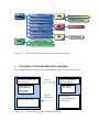
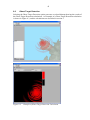
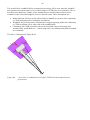
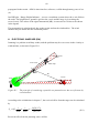
OVERALL DESCRIPTION
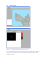
Figure 3.1
Results
Ojects
Geo info
WIMP (1) is used as a tool to enter objects used in the analysis and to present results from the
analyses. The project entered in WIMP will be stored in an xml-file. WTES reads the actual
xml file(s) and executes the selected calculations and analysis. To visualize the results of these
calculations and analysis, WTES generates an xml file and accompanying bitmap file, as
described later in this report (chapter 4).
Overview of the different programs involved.
The WTES includes all the blocks in the middle and right of Figure 3.1. The calculation
opportunities are shown in Figure 3.2.
The WTES is implemented in LabVIEW 8.2. The code is based on event handling and event
queuing. The executable code will be independent of having LabVIEW installed at your
computer (see chapter 5).
The Graphical User Interface is organized with pull-down menus and push buttons. The
results are shown in WTES, or written to files for presentation in WIMP.
11
Visibility
Second Reflections
Primary Reflections
Ghost Target
Second Reflections
APM
Exclusion Zone
RCS
Shadow Effects
Jamming Effects
Scattering
Signal Level
Ghost Target Detection
Figure 3.2
4
The calculation opportunities for the different modules.
EXCHANGE OF DATA BETWEEN WTES AND WIMP
The communication is done by use of xml and bitmap files, as shown in Figure 4.1.
Generate or load project
Save project
xml file
Execute calculations
Execute analysis
WTES
MARIA/
WIMP
xml file
bitmap file
View results on map
Figure 4.1
View results
Generate bitmap file
and xml file
Communication between WIMP and WTES
12
4.1
Reading WIMP data
WTES reads data from xml file(s) stored in WIMP. The xml file contains objects and
attributes, and the format of the xml file is given in (1).
The data are stored in global LabVIEW variables, containing clusters of data. The data are
used in calculations, analysis and presented to the user.
4.2
Writing WIMP data
WTES can make changes to existing projects and save the updated project. The object data
including their attributes will be written to an xml file according to the format described in (1).
5
INSTALLING WTES
The DVD contains DTED Map, Run LabVIEW_8.2_Runtime_Engine.exe and WTES
Installer.exe.
1) Copy the DTED Map folder to your computer (this path must be set in WTES main
settings, see section 6.1 and Figure 6.4)
2) Run LabVIEW_8.2_Runtime_Engine.exe
3) Run WTES Installer.exe
6
USER MANUAL
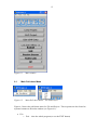
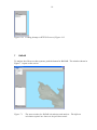
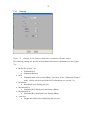
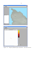
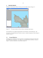
Starting the WTES program gives the main window shown in Figure 6.1.
13
Figure 6.1
6.1
Main window
Main Pull-down Menu
Figure 6.2
Main Pull-down Menu – File and Project
Figure 6.2 shows the pull-down menu for File and Project. These options are also found as
separate buttons on the main window (see Figure 6.1).
•
File
o Exit – close the whole program (or use the EXIT button)
14
•
Project
o Load – loads a project (see 6.2.1)
o Save – saves a project (see 6.2.2)
o Edit – Edit WIMP Data (see 6.2.3)
Figure 6.3
Main Pull-down Menu – Tools and Help
Figure 6.3 shows the pull-down menu for Tools and Help
•
•
Tools
o Settings (see below)
o Restore Default Settings – restores all default settings
Help
o About (see below)
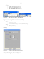
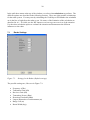
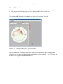
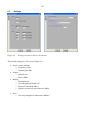
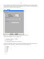
Settings:
Figure 6.4
Settings in Main Menu (Default values).
The possible settings are, like seen in Figure 6.4:
15
•
•
•
•
DTED Map Source
Tells WTES where the DTED map data are stored
DTED Level
Gives the resolution of the map, DTED2 gives the best resolution
Map Start Bound
The coordinates of the map (WGS84) (Default values gives Norway).
Map Matrix Size
The size of the map shown in WTES (in pixels)
Help:
Figure 6.5
6.2
About WTES.
Project handling
The project handling may be done by the main pull-down menu or the buttons on the main
window.
6.2.1
Load
Loads the xml-file from WIMP, the format of this file is given in (1). The objects attributes
may be changed in the Edit WIMP Data.
6.2.2
Save
Saves an xml-file from WTES, the format of this file is given in (1). If two or more projects
are loaded into WTES, they are stored together in one xml-file by SAVE.
6.2.3
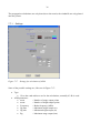
Edit WIMP Data
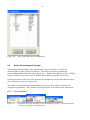
A new window opens and shows the WIMP data in tables. Select the actual object from the
list by double click the name. Another window opens showing the parameters for the chosen
object as shown in Figure 6.6. Change the desired parameter(s) and push OK. The updated
data can be saved by pushing the SAVE Project button (Figure 6.1).
16
Figure 6.6
6.3
Show, add, edit and save WIMP data.
Select Electromagnetic System
After locating the map (Figure 6.4) and loading a project (section 6.2.1) select the
electromagnetic system you want to analyze. The selection is done by pushing the
corresponding button in the main menu (Figure 6.1). Radar is described in section 7, SSR in
section 8, Passive sensors in section 9, Radio Link in section 10 and HF in section 11.
If no map is shown in the view of the selected electromagnetic system, check that the link to
your map data is correct (see Figure 6.4).
The windows for the different electromagnetic system are rather similar, except for the
calculation opportunities. They all have a pull-down menu as described in the subsections.
6.3.1
Pull-down Menu
Figure 6.7
Pull-down menu for the different electromagnetic systems. Calculation menu
will vary according to selected system.
17
Figure 6.7 shows the pull-down menu for all the electromagnetic systems
•
•
•
•
6.3.2
File
o Save MARIA Bitmap (see section 6.4)
o Save MARIA Bitmap As .. (see section 6.4)
o Exit – exit this electromagnetic system and return to the main window.
Calculations
o See the description of the different electromagnetic systems (section 7-11).
Map
o Zoom In – zoom the map in
o Zoom Out - zoom the map out
o Revert to Default – revert to the latest saved map settings
o Save as Default Map – save current settings as default map settings (using the
Restore Default Settings (6.1) will overwrite these settings)
Tools
o Settings – described for the different electromagnetic systems (section 7-11).
Mouse Menu
The mouse menu is different in the Map area and the Plot & Curves area.
In the Map area:
Right clicking the mouse gives a menu
•
•
•
Centre Map
Zoom In
Zoom Out
In the Plot & Curves area:
Moving the mouse onto the bitmap shows a short description (tip strip) for the bitmap.
Right clicking the mouse gives a menu
•
•
•
Copy Data
Description and Tip ..
Smooth Updates
By selecting the Description and Tip .. you see a description for the bitmap together with the
short description (Tip). You may copy the bitmap window by selecting Copy Data and choose
whether you want Smooth Updates or not.
18
6.3.3
Radars and Windmills
If your project has more than one radar and/or wind farm you have to select which one to do
the calculations on. This is done by selecting the tab “Plots & Curves”, and then select the
desired radar/windmill as shown in Figure 6.8.
Figure 6.8
6.4
Select the radar/windmill to do calculations on.
Saving WTES bitmaps
The bitmaps results form the different calculations in WTES appears in the Bitmaps list as
Current (see Figure 6.9). You may save the bitmap to be able to view it in the chart display on
WIMP/Maria or to recall it in the WTES later for instance to compare to other bitmaps. To
save a bitmap, select the “File” option in the main pull-down menu (section 6.1). The program
then generates two files with the same name but different extension; an xml file describing the
position, size and orientation and the bitmap file. The format of the file is described in (1).
Default file name and file location may be set in Settings for the different calculations.
Figure 6.9
Saving bitmaps in WTES. Extract of Figure 7.3 .
To load a stored bitmap, push the Load button (see Figure 6.10). Many bitmaps can be in the
list at the same time and you may choose which one to be shown in the map by marking the
actual bitmaps.
19
Figure 6.10 Loading bitmaps in WTES. Extract of Figure 10.2.
7
RADAR
To analyze the effects on radar systems, push the button for RADAR. The window shown in
Figure 7.1 opens on the screen.
Figure 7.1
The menu window for RADAR calculations and analysis. The different
calculation options are shown in the pull-down menu.
20
In the pull-down menu at the top of the window you select what calculations to perform. The
different options are described in the following sections. There are eight possible calculations
for the radar system. You may start by calculating the Visibility to find whether the windmills
are in the line-of-sight from the radar or not. Be aware of the limitation of the calculation as
described in A.1. If visible, use the WF Impact overview to get an overview of the situation.
Use the other calculation option to evaluate the situation and demonstrate the different
influences to the radar.
7.1
Radar Settings
Figure 7.2
Settings for the Radar (Default settings).
The possible settings are, like seen in Figure 7.2:
•
•
•
•
•
•
•
•
Frequency (GHz)
Transmitter Gain (dB)
Receiver Gain (dB)
Transmitter Power (dBm)
Detection Threshold (dBm)
Largest Dimension of radar antenna (m)
Range Cell (m)
Beam Width (deg)
21
These settings are used for all the radar calculations. In addition other parameters are set in
local settings for the different calculations (according to the different tabs on the settings left
side, see Figure 7.2).
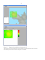
7.2
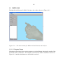
Visibility
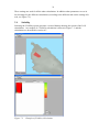
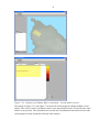
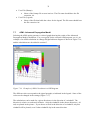
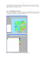
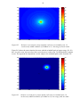
Selecting the Visibility option generates a colored bitmap showing the results of the LOS
calculations. An example of a Visibility calculation is shown in Figure 7.3, and the
calculations are described in section A.1.
Figure 7.3
Example of Visibility Calculation
22
The calculations prepare a bitmap file, using different colors to indicate whether the various
wind turbines are not visible (green), partly visible (yellow) or completely visible (red). These
are solely based on Line-of-sight calculations according to terrain, but not according to signal
deflection, as described in chapter A.1.
7.2.1
Settings
Figure 7.4
Settings for the calculations of visibility (Default settings).
The possible settings are, like seen in Figure 7.4:
•
•
•
Bitmap resolution
The resolution of the plot.
LOS Calculation Limits
The limits are automatically calculated from the wind farm area, as described in
chapter A.1. The limits may be changed manually.
LOS Calculation Resolution
The resolution of the calculations, as described in chapter A.1.
23
7.3
Windfarm Impact Overview
Figure 7.5
Example of WF Impact Overview diplay showing range and azimuth extent of
severely affected area (CFAR/C-map and false target) plus the two range rings
(absolute range limit and minimum range of calculation validity)
24
This calculation assumes that the wind park is within line-of-sight of the radar (see section
7.2).
The WF Impact Overview module calculates the area of severe radar influence by the wind
park. The module produces a range and azimuth limited sector around the windmill park where
false targets may appear due to false detections from the rotors or double reflections off the
wind park and real targets, and where targets may be lost due to deteriorated CFAR or clutter
map processing performance. The range rings show whether or not the specific situation being
analysed is within the validity area of the module. Within the innermost range ring the
calculations loose all validity, and between the innermost and outermost range ring additional
evaluations such as on-site experiments should be performed.
Calculations and assumptions used for this module are shown in chapter B.
7.3.1
Settings
The radar settings are shown in Figure 7.2, an extract is shown in Figure 7.6.
Figure 7.6
Extract of radar settings (Figure 7.2) actual for the WF Impact Overview
(Default values).
The possible parameter settings are, as seen in Figure 7.6:
•
•
•
Largest Dimension
Range Cell
Bean Width
Based on the parameters the Impact Zone is given by:
•
•
Range affected area = wind park range extent + Range Cell in both directions
o Should reflect actual radar clutter map or CFAR range extent
Azimuth affected area = wind park azimuth extent + 1 antenna beam width in both
directions
o Should reflect actual radar clutter map or CFAR azimuth extent
The Absolute Near Field is, according to the discussion in B:
•
Inner range ring radius = 1 km.
The Near Field is given by:
•
Outer range ring radius = 5 D 2 λ where D is the Largest dimension and λ is the
wavelength.
25
7.4
Primary reflections
Selecting the Primary Reflections option generates a colored bitmap showing the results of the
Primary Reflections calculations. An example of a Primary Reflections calculation is shown
in Figure 7.7. The theory is described in section C.
Figure 7.7
Example of a Primary Reflections calculation. Selected mode is Windmill RCS.
26
It is possible to choose between two different modes for the calculations:
1) Windmill RCS:
Calculates the RCS required for the windmill to be detected by the radar at a given distance
(assuming free line of sight between the radar and the windmill). See Figure 7.7.
2) Minimum Distance:
Calculates the minimum required distance between the radar and a windmill with given RCS
(see settings in Figure 7.9) in order for the radar not to detect the windmill (assuming free line
of sight between the radar and the windmill). Areas where the radar can detect the windmill are
shown in red colour, while areas where the radar cannot detect the windmill are shown in
green. See Figure 7.8.
Figure 7.8
Example of a Primary Reflections calculation. Selected mode is Minimum
Distance.
27
7.4.1
Settings
Figure 7.9
Settings for the Primary Reflections calculations (Default values).
The following settings are specific to the Primary Reflections calculations (see also Figure
7.2):
•
•
•
•
•
•
Mode (See section 7.4):
Windmill RCS
Minimum Distance
RCS
Windmill radar cross section (dBsm). Used only for the “Minimum Distance”
mode. Values may be found in the RCS calculations (see section 7.8).
Resolution
Resolution of the bitmap grid (m).
Minimum RCS
Minimum RCS displayed in the bitmap (dBsm).
Maximum RCS
Maximum RCS displayed in the bitmap (dBsm).
Area Size
Height and width of the bitmap/targeted area (m).
28
7.5
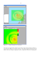
Second Reflection
Selecting the Second Reflection option generates a colored bitmap showing the results of the
second reflection calculations. An example of a Second Reflection calculation is shown in
Figure 7.10, and the calculations are described in section D.
Figure 7.10 Example of Second Reflection Calculation – Target RCS mode.
The calculation is done according to a certain target altitude, chosen in the settings (Figure
7.12).
29
By selecting the mode Target RCS, the lowest necessary RCS value for a target, in a given
altitude and position, to be detected by the radar is calculated. This is done for every position
in the defined area and for each windmill. The result in each of the positions is the lowest
value calculated for the different windmills. The result is divided into five levels; red, orange,
yellow, light green and dark green. Green corresponds to a low necessary RCS, while red
corresponds to a high necessary RCS.
Figure 7.11 Example of Second Reflection Calculation – Ghost target detection mode.
30
By selecting the mode Ghost target detection, the calculated necessary RCS values are
compared to a threshold-value, set by the Actual Target RCS in settings (see Figure 7.12). The
pixels containing RCS values below the threshold are red, the other are blank. This means that
targets having RCS equal to or below the threshold and being in the red positions, will
generate ghost targets behind the wind park.
7.5.1
Settings
Figure 7.12 Settings for calculations of second reflections (Values used in example).
Some of the possible settings are, like seen in Figure 7.12:
•
•
•
Mode:
Target RCS
Ghost Target Detection
Target altitude
The calculations are done for the given target altitude. Change the parameter to
make calculations for other altitudes.
Actual Target RCS
The typical RCS of the interested targets. Used in the Ghost target detection
mode as the threshold value.
31
7.6
Shadow Effects
Selecting the Shadow Effects option generates a colored bitmap showing the results of the
Shadow Effects calculations. An example of a Shadow Effects calculation is shown in Figure
7.13 and Figure 7.14. The theory is described in section E and in (3).
It is possible to choose between four different modes for the calculations:
1) Fast:
This is the fastest option. Calculates and plots the dark shadow region behind the windmill.
Calculations are based upon Equations (E.7)-(E.17). The shadow is plotted for all wind
turbines in the wind park.
2) Custom:
For showing the electromagnetic field both inside and outside of the dark shadow region, this
is the fastest option. Based on the given frequency a bitmap of fixed size (500x1000 m) and
resolution (2 m) is chosen from a library of previously generated bitmaps. Equations (E.1)(E.6) have been used for the calculations. The bitmap is shown for one wind turbine, but the
results are similar for the other wind turbines.
3) User Defined:
Calculates the electromagnetic field both inside and outside of the dark shadow region. Values
for all parameters are set by the user (see Figure 7.15). Calculations may take from a few
minutes up to several hours depending on the choice of frequency and the size and resolution
of the targeted area (bitmap). Equations (E.1)-(E.6) are used in the calculations. The bitmap is
shown for one wind turbine, but the results are similar for the other wind turbines.
4) User File:
Shows a previously user generated bitmap (see 3) above).
32
Figure 7.13 Example of Shadow Effect calculations – Fast mode selected.
33
Figure 7.14 Example of a Shadow Effects calculation – Custom mode selected.
The bitmap in Figure 7.13 and Figure 7.14 shows the electromagnetic shadow behind a wind
turbine. The electric field is calculated relative to the unperturbed electric field (when the wind
turbine is not present). The calculations do not take into consideration interactions between the
electromagnetic fields around the different wind turbines.
34
7.6.1
Settings
Figure 7.15 Settings for the Shadow Effects calculations (Default values).
The following settings are specific to the Shadow Effects calculations (see Figure 7.15):
•
•
•
•
•
•
•
Mode (See section 7.6):
Fast
Custom
User defined
User File
Maximum tower radius
Maximum tower radius (m).
Resolution
Resolution of the bitmap grid (m).
Minimum Electric Field
Minimum electric field displayed in the bitmap (dBV/m).
Maximum RCS
Maximum electric field displayed in the bitmap (dBV/m).
Area Size
Height and width of the bitmap/targeted area (m).
User File Path
The path to the location that user files will be stored/retrieved from.
35
•
•
7.7
User File (Bitmap)
Name of the bitmap-file to store/retrieve. The file name should have the file
extension .ini.
User File (Legend)
Name of the file that holds the values for the legend. The file name should have
the file extension .ini.
APM - Advanced Propagation Model
Selecting the APM option generates a colored graph showing the results of the Advanced
Propagation Model calculations. For a user guide for the external APM program, see (6). An
example of an APM calculation in a Range-Height-Indicator diagram is shown in Figure 7.16,
and the calculations are described in section G.
Figure 7.16 Example of APM Calculation in a RHI diagram.
The different colors correspond to the signal strength, as indicated in the legend. Some of the
colors can be changed in the settings (Figure 7.17).
The calculations can be made for a given direction or in the direction of a windmill. The
direction is relative to north and clockwise. Only the windmills in the chosen direction (± 0.1
rad) are plotted in the picture. If you choose to look in the direction of a windmill, only this
windmill will be plotted, even if other windmills lay in the same direction.
36
The propagation calculations are only done due to the terrain; the windmills are only plotted
onto the picture.
7.7.1
Settings
Figure 7.17 Settings for calculation of APM.
Some of the possible settings are, like seen in Figure 7.17:
•
•
Type
Gives the earth radius to use for the calculations, normally 4/3 Re is used.
APM parameters
nrout
= Number of range output points
nzout
= Number of height output points
Frequency
= Radar frequency (MHz)
Hg max
= Maximum height output (m)
Hg min
= Minimum height output (m)
Rg
= Maximum range output (km)
37
7.8
RCS-model
Simulations are accomplished for two different generic windmills (data are given in appendix
F). The program will automatically chose the predefined RCS model with best
correspondence to the actual windmills.
The predefined RCS models of windmills are described in section F and (4).
Figure 7.18 Example of RCS for a given elevation.
Select windmill (nr according to place in the xml-file) and percentile value. The program
calculates the elevation angle between the radar and the chosen windmill. The RCS values for
the most relevant generic windmill are shown.
38
7.8.1
Settings
Figure 7.19 Settings for plotting of RCS data (Default values).
The possible settings for RCS calculations are, as shown in Figure 7.19:
•
•
7.9
Percentile Threshold (%).
Plot colours.
Jamming Effects
Selecting the Jamming Effects option generates a colored bitmap showing the results of the
Jamming Effects calculations. An example of a Jamming Effects calculation is shown in
Figure 7.20, and the calculations are described in section H.
39
Figure 7.20 Example of Jamming Effects.
The different colors indicate the necessary RCS of a target to be detected in the different
positions under influence of jamming. The settings possible to adjust, is shown in Figure 7.21.
40
7.9.1
Settings
Figure 7.21 Settings for calculation of Jamming Effects.
Some of the possible settings are, like seen in Figure 7.21:
•
•
8
Jamming source
o Effect (W)
o Gain
o Frequency (GHz)
o Elevation angle (Jammer-windmill) (deg)
Miscellaneous
o Angular resolution (deg)
o Distance to target (m)
o RCS of target (m2)
o RCS colour scheme (colour for the five levels of target RCS)
SECONDARY SURVEILLANCE RADAR (SSR)
Pushing the radio button for SSR gives the window shown in Figure 8.1.
41
Figure 8.1
The menu window for SSR calculations and analysis
For the SSR there are two different opportunities for calculations, as described below. The
description of Signal Level is found in section 8.1 and the description of Ghost Target
Detection is found in section 8.2.
8.1
Signal Level
Selecting the Signal Level option generates a colored bitmap showing the results of the Signal
Level calculations. An example of a Signal Level calculation is shown in Figure 8.2, and the
calculations are described in section I.
42
Figure 8.2
Example of Signal Level Calculation
The colours correspond to the signal level received by a target in this position according to a
request from the SSR received via the wind farm. The signal strength is divided into 5 levels,
and the colours are dark green, light green, yellow, orange and red (form low to high signal).
43
8.2
Ghost Target Detection
Selecting the Ghost Target Detection option generates a colored bitmap showing the results of
the Ghost Target Detection calculations. An example of a Ghost Target Detection calculation
is shown in Figure 8.3, and the calculations are described in section I.
Figure 8.3
Example of Ghost Target Detection Calculation
44
When the signal level received by the target is above the sensitivity of the transponder, the
transponder will reply, and a ghost target is detected. The true target in the indicated position
will give a ghost target behind the wind farm. The sensitivity or detection threshold is given in
settings (Figure 8.4).
8.3
Settings
Figure 8.4
Settings for SSR calculations.
The possible settings are, like seen in Figure 8.4:
•
•
•
•
Secondary Surveillance Radar Antenna
Frequency (GHz)
Transmitter Power (dBm)
Antenna Gain (dB)
Aircraft (Target)
Altitude (m)
Receiver Gain (dB)
Bitmap
Resolution (m)
Height and Width of the calculated bitmap (m)
Detection threshold (dBm)
Maximum signal level (dBm)
Minimum signal level (dBm)
Misc
One-way atmospheric attenuation (dB/km)
45
9
PASSIVE SENSOR
Pushing the radio button for Passive Sensor gives the window shown in Figure 9.1.
Figure 9.1
The menu window for Passive Sensor calculations and analysis
For the PS there are two different opportunities for calculations, as described below. The
description of Second Reflection is found in section 9.1 and the description of Ghost Targets is
found in section 9.2.
9.1
Second Reflection
Selecting the Second Reflection option generates a colored bitmap showing the results of the
Second Reflection calculations. An example of a Second Reflection calculation is shown in
Figure 9.2, and the calculations are described in chapter K.
46
Figure 9.2
Example of Second Reflection Calculation for PS.
The signal level received at the passive sensor caused by a signal transmitted from an emitter
in the actual position reflected via the wind park is calculated.
47
9.2
Ghost Targets
Figure 9.3
Example of Ghost Targets Calculation for PS.
For every possible emitter position, inside a defined area, the calculations give whether the
signal received at the passive sensor is above the detection threshold. If so, the emitter
position is shown red.
48
9.3
Settings
Figure 9.4
Settings for Passive Sensor calculations.
The possible settings are, like seen in Figure 9.4:
•
•
•
•
Passive sensor antenna:
o Frequency (GHz)
o Antenna gain (dB)
Emitter
o Altitude (m)
o Power (dBm)
Bitmap
o Resolution (m)
o Area (Height and Width) (m)
o Detection Threshold (dBm)
o Signal level interval (min and max) (dBm)
Misc
o One-way atmospheric attenuation (dB/km)
49
10
RADIO LINK
Pushing the radio button for Radio Link gives the window shown in Figure 10.1.
Figure 10.1 The menu window for Radio Link calculations and analysis
10.1.1 Exclusion Zones
Selecting the Exclusion Zones option generates a colored bitmap showing the results of the
Exclusion Zones calculations. An example of an Exclusion Zones calculation is shown in
Figure 10.2, and the calculations are described in section J.
50
Figure 10.2 Example of Exclusion Zones Calculation
The exclusion zones are composed of a near field area around each radio (see section J.1) and a
fresnel zone around the link (see section J.2 and J.3). To avoid corruption of the signal, the
signal path directly between the radios and the signal path via the windmill should differ less
than λ (se equation (J.)).
To avoid signal corruption or obstruction, the windmills must be outside the read area.
51
10.2
Settings
Figure 10.3 Settings for calculation of Exclusion Zones.
The possible settings are, like seen in Figure 10.3:
•
•
•
11
The Radio Antenna
Efficiency (between 0 and 1)
Frequency (GHz)
Boresight Gain (dB)
Aperture diameter (m)
Aperture known (yes/no)
Miscellaneous
Worst-case RCS of Windmill (m2)
Minimum Carrier-to-Interference ratio (dB)
Bitmap
Resolution (m)
HIGH FREQUENCY (HF)
Pushing the radio button for HF gives the window shown in Figure 11.1.
52
Figure 11.1 The menu window for HF calculations and analysis
The HF module applies to passive sensors in the frequency range 740 kHz – 30 MHz. Passive
sensors in higher frequency bands should be handled by the Passive sensor module.
11.1
HF Scattering – far field
Selecting the HF Scattering Far Field option generates a colored bitmap showing the results of
the far field calculations. An example of a HF Scattering Far Field is shown in Figure 11.2,
and the calculations are described in (7) and (8).
Figure 11.2 Example of HF Scattering Far Field Calculation
53
Presented bitmap for far field calculations shows the ratio Ks between the direct scattered
signal and the reflected signal in dB. The far field bitmap show Ks as a function of azimuth
angle of incidence (0 = North, 90 = East).
11.2
HF Scattering – near field
Selecting the HF Scattering Near Field option generates a colored bitmap showing the results
of the near field calculations. An example of a HF Scattering Near Field is shown in Figure
11.3, and the calculations are described in (7) and (8).
Figure 11.3 Example of HF Scattering Near Field Calculation
54
Presented bitmap for near field calculations shows the ratio Ks between direct scattered signal
and the reflected signal in dB. The near field bitmap gives Ks as a function of azimuth angle of
incidence and Tx position within the inner area.
11.3
Settings
Figure 11.4 Settings for HF Scattering calculations (Default values).
The possible settings are, like seen in Figure 11.4:
•
•
•
Frequency (740 kHz – 30 MHz)
RCS of windmill
Conductivity Ground (mS/m2)(see Figure L.)
As long as the parameter Conductivity Ground is Undefined, the program will prompt the user
to select one of the valid values. Valid values for Norway is (see Figure L.1):
•
•
•
•
•
•
•
0,0001
0,0003
0,001
0,003
0,01
0,03
5
55
12
SUMMARY
This report describes the software tool WTES developed at FFI to assist the Norwegian
Defense in the management of Wind Turbine development applications.
The software tool will support the consideration of the applications for the Defence based on
the theoretical presumption described in the latter chapters. The software will not give the
answer of the application, but will give the action officer a better qualification to make the
decisions.
13
ACKNOWLEDGEMENTS
The authors wish to extend their thanks to the following persons: Hans Øhra who initiated the
project and was the project manager from the start in November 2004 until October 2006,
Morten Søderblom at FFI who simulated the RCS data and Roald Otnes for developing the
models for HF scattering. We also wish to thank the “Tiger Team” established in December
2006 to support the project in the final month. The FFI internal team was consisting of SveinErik Hamran, Terje Johnsen, Trygve Sparr, Aanund Storhaug, Steffen Tollisen and Stein
Kristoffersen.
56
References
(1)
Bente Jensløkken Meland, Hans Øhra (2007): Windfarm Impact on Electromagnetic
Systems (WIMP) – Software Documentation, FFI/RAPPORT-2007/00832
(2)
Yngve Steinheim, Stig Petersen (2004): Analysis of possible consequences of
collocating Avinors Monopulse Secondary Surveillance Radar and wind turbines at
Urdalsnipa, Sintef report STF90 F04035 (Confidential)
(3)
Gudrun Høye (2007): Electromagnetic shadow effects behind wind
turbines,FFI/RAPPORT-2007/00842
(4)
Morten Søderblom (2007): RCS simulation of wind turbines, FFI/RAPPORT2007/00896
(5)
Hans Øhra (2003): Vindkraftverks konsekvenser for Forsvarets installasjoner Innledende studie for radar, FFI/RAPPORT-2003/02784
(6)
(APM): http://www.spawar.navy.mil/sti/publications/pubs/td/3145/td3145.pdf.
(7)
Otnes, Roald (2007): Modelling of Electromagnetic Influence fram Wind Farms at
Frequencies below 30 MHz - Interference and scattering, FFI/RAPPORT-2007/00086
(8)
Otnes Roald, Hjelmstad Jens (2006): Observability at HF direction finding sites of
scattering from wind farms - measurements at Smøla 2006, FFI/RAPPORT-2006/02701
(9)
Steffen Tollisen, Aanund Storhaug (2007): Wind farm impact assessment on radars in
the North-Cape area, FFI/NOTAT-2007/00793
(10) (1999): Rec. ITU-R P-832-2: World Atlas of Ground Conductivites.
57
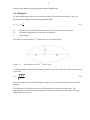
A
GEOMETRY
The basic calculations of geometry are mostly organized in the library files. Positions are
given in latitude, longitude and height of WGS84.
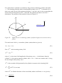
A.1 Line-of-sight (LOS)
LOS is calculated based on dted height data. The LabVIEW program gathers height profile
data for an area as shown in Figure A.1. The data must be collected with dense sampling in
angle. For each height profile, calculations are made step by step to estimate the highest point
possibly seen by the radar. The principle of screened height is shown in Figure A.2.
The LOS calculations does not account for the radar signal propagation. the propagation
effects are given by the APM module (see section 7.7).
Figure A.1
Start and stop angle for the area seen from the radar.
Figure A.2
The principle of screened height.
58
B
RADAR IMPACT OVERVIEW
The WF Impact Overview module encompasses two effects that windmills may have on a
radar:
1. Reflections via the windmill park where real targets may result in false targets with
apparent different position than the original target.
2. Increased clutter levels in automatic detection processing such as clutter maps and
CFAR.
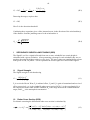
The first situation is illustrated in Figure B., where a reflection of the radar Tx signal via the
windmill (blue star, σw), to the real target (green target, σT), and back via the windmill results
in a false target at a position directly behind the windmill (pink target).
4
PRT =
4
σW
ERP
σT
(4π RT2 ) 2
σT
RWT
RT
PRWT =
=
ERP
1
1
1
σ WT
σT
σ TW
2
2
2
4π RW
4π RWT
4π RTW
4π RW2
2
ERP ⋅ σ T σ WT
4
(4π ) 4 RW4 RWT
RW
2
σ WT
PRWT
RT4
RT4
2
σ WT = 4
=
4
(4π ) 2 RW4 RWT
PRT
RWT (4π ) 2 RW4
Figure B.1
Reflections via windmill.
Figure B.1 also contains the equations to calculate the relative received power level from the
double reflection case, PRWT/PRT. PRWT/PRT is the power received via the double reflection
when the antenna points at the windmill, relative to the power received from the direct path to
the target when the antenna points directly at the target. It is a measure of how strong a false
target a given real target may produce.
PRWT/PRT = -30dB means that a target in this position with an RCS of 30dBsm would result in a
false target behind the windmills of 0dBsm. A reasonable threshold for PRWT/PRT could be -50
dB, which means a 10.000 m2 real target could result in 0,1 m2 false target in another position.
The equations above (Figure B.) does not take into account the fact that many radars adjust
their sensitivity as a function of the range to a target, so called STC – Sensitivity Time Control.
The range to the real target generating the false target is generally shorter than the range to the
false target, so the power ratio of Figure B. should be adjusted with the appropriate range
factor. Assuming a perfect R4 STC regime, PRWT/PRT should be multiplied by
(RW + RWT)4/RT 4.
Figure B.2 shows a calculation of the equations above using σw = 50 dBsm. The radar is at
(0,0) and the windmill park is at (10, 10) km. Figure B. shows that only real targets within a
few kilometres from the windmill park can generate false targets above the -50 dB threshold.
59
100
-30
80
-35
60
-40
40
-45
20
-50
0
-55
-20
-60
-40
-65
-60
-70
-80
-75
-100
-100
Figure B.2
-50
0
50
100
-80
Relative received power from a double reflection via windmill park, 16
incoherently added windmills of 50 dBsm at 14,1 km range from the radar.
Figure B.3 shows the same situation, but now with the windmill park at longer range; (50, 50)
km. As can be seen, the area where the received power is above the -50 dB threshold is similar
in size. The apparent low dependence on the range to the windmill park results from the STC.
100
-30
80
-35
60
-40
40
-45
20
-50
0
-55
-20
-60
-40
-65
-60
-70
-80
-75
-100
-100
Figure B.3
-50
0
50
100
-80
Relative received power from a double reflection via windmill park, 16
incoherently added windmills of 50 dBsm at 14,1 km range from the radar.
60
The second effect, windmill effects on detection processing, will be seen when the windmill
park produces increased clutter levels in clutter maps or CFAR noise level estimation. This is
not analyzed in detail here. Rather, some assumptions are described that result in course
estimates on the effects that might be seen on a specific radar. These assumptions are:
•
•
•
Radar detection will be severely affected when windmills are present in the cluttermap
or CFAR background level estimation calculations.
Windmills are present in these calculations for targets appearing within one cluttermap
or CFAR resolution cell to either side of the windmill park.
Cluttermap and CFAR resolution cells can be described using a fixed range and
azimuth value, and defaults of ± 1 km in range and ± one antenna beamwith in azimuth
are reasonable.
The above is illustrated in Figure B.44.
RCAFR/C-map
θaz
θaz
RCAFR/C-map
θaz
Figure B.4
Area where a windmill park will affect CFAR and cluttermap detection
performance
61
θaz
Figure B.5 Ranges where assumption may not be valid
Figure B.5 above shows two range rings around the radar. These are also included in the
WTES WF Impact Overview module (section 7.3) to point to the fact that all calculations and
discussions in this section assumes far field free space conditions. If the windmills are within
the innermost ring (dark red) they are well within the radar near field. In that case most of the
discussions above are not valid. The exact range to the near field limit is not possible to
determine exactly, since the transfer from near filed to far field is continuous. Even so, a
reasonable estimate could be that windmills within a range of 1 km off a radar will produce
near field effects that are very difficult to estimate in any detail. Windmills should not be
placed within this range without very careful evaluation, and preferably on-site experiments
using synthetically generated signals to simulate windmill effects.
The outer range ring is there to point to the fact that there is a transition region where the
calculations and discussions above are very uncertain, especially in terms of magnitude of the
effects the wind park may have. This uncertainty may go in both directions, but at close range
between the radar and the wind park (e.g. less than 5 or 10 km) special care should be taken,
and other effects than the ones described above may dominate. The quality and fidelity of these
calculations do not allow for evaluation of closely separated radar and windmill sites. Again
on-site experiments are suggested.
C
PRIMARY REFLECTIONS
The strength of the reflected signal is important for the evaluation on the wind turbines
influence on the radar (5).
An electromagnetic signal, with an effect Pt sent from an antenna with gain Gt , will at a range
of Rt from the transmitter have the power density
62
St = PG
t t
1
4π Rt2
(W m 2 )
(C.1)
When the signal hits an object, the received effect will be scattered in different directions. The
transmitted effect is
Pσ = Stσ
(W )
(C.2)
when σ is the targets radar cross section.
In the distance Rr from the object the power density of the reradiated effect, Pσ , can be
calculated similar to (C.1):
Sσ = Pσ
1
4π Rr2
(W m 2 )
(C.3)
The received signal effect of a receiver antenna with an effective area, Ae , receive this signal,
will be
Pr = Sσ Ae
(W )
(C.4)
The effective area of the receiver may be expressed by the antenna gain, Gr :
Ae =
Gr λ2
4π
(C.5)
where λ is the signals wavelength. By combining the equations (C.2), (C.3), (C.4) and (C.5),
the effect in the receiver will be
Pr =
Pt Gt Gr λ2σ
(4π )3 Rt2 Rr2
(W )
(C.6)
To be able to detect the object, with some simplifications, the effect, Pr must satisfaction the
following hypothesis:
H0 :
Pr < PD
object is NOT detected
H1 :
Pr ≥ PD
object is detected
(C.7)
where PD is the necessary effect to detect a target.
In the purchase of a monostatic radar system, the minimum detection range, R0 , for a given ,
σ 0 ,(usually 1 m2), is often specified. The received effect for monostatic radars is then
63
PD =
2
PG
t t Gr λ σ 0
( 4π )
3
(W )
R04
(C.8)
The maximum detection range for monostatic radars is then
⎛ PG G λ 2σ
R = ⎜ t t r3
⎜ ( 4π ) P
D
⎝
1/ 4
⎞
⎟
⎟
⎠
(m)
(C.9)
In this equation the radar designer controls all the parameters except the radar cross section σ .
Equation (C.9) can also be used to calculate the radar cross section σ D that is required for a
target to be detected at distance R
σD =
D
(4π )3 PD R 4
2
PG
t t Gr λ
(m 2 )
(C.10)
SECOND REFLECTIONS
The calculations for the Second Reflections are much the same as for the SSR described in
section I. The difference is that you calculate the Radar Cross Section (RCS) any possible
target must have to be detected as a ghost target when the signal is reflected from a windmill.
This is done by
4
4
P0 ( 4π ) Rw Rwt
σt =
Pt Gt Gr λ 2σ w
5
(D.1)
This is a variation of the equation (5.2) in (5). P0 is the signal strength needed at the receiver
to detect a target, Pt is the signal strength radiated, Rw is the range from the radar to the
windmill, Rwt is the range from the windmill to the target, Gt og Gr is the gain at transmitter and
receiver respectively, λ is the wavelength and σw is the windmill RCS.
Low RCS corresponds to ”worst-case”, and the colour scale is chosen so that red corresponds
to a low necessary RCS, while green corresponds to a high necessary RCS. Every pixel in the
bitmap will be the lowest necessary RCS value for every windmill.
E
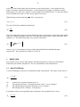
SHADOW EFFECT
When an electromagnetic wave is obstructed by an object that has a size comparable with the
wavelength, the electromagnetic wave is diffracted and creates a shadow region behind the
object. This will be the case when a wind turbine (size of several meters) is obstructing the
electromagnetic wave from a radar (wavelength of centimeters to meters).
64
The wind turbine is modeled as an infinitely long perfectly conducting cylinder with radius
rcyl . The incoming (from the radar) electromagnetic primary wave Ezprim is assumed to be a
plane wave with electric field component along the z -axis only, and it is also assumed that the
electric field is homogeneous in the z -direction. The problem can then be solved in 2
dimensions. The geometry of the problem is shown in Figure E.1.
y
Hy
r
Primary wave
Ez
rcyl
φ
x
Figure E.1
Diffraction on a conducting cylinder of infinite length (cross-section in the xyplane).
The total electric field Eztot around the cylinder (wind turbine) is given by
Eztot = Ezprim + Ezsec
(E.1)
Here Ezprim is the incoming primary field
Ezprim = E0 e jkr cosϕ
(E.2)
where E0 is the electric field amplitude of the primary wave, r is the distance from the
cylinder, ϕ is the angle around the cylinder, and k = 2π / λ is the wave number with λ being
the wavelength of the primary wave.
Ezsec is the secondary field generated by the cylinder in response to the incoming field
∞
Ezsec = ∑ Am H m(2) (kr ) cos(mϕ )
(E.3)
m=0
where H m(2) are Hankel functions of the second kind, and the coefficients Am are given by
A0 = −
E0 J 0 (krcyl )
H 0(2) (krcyl )
(E.4)
65
and
Am = −2 j m E0
J m (krcyl )
(E.5)
H m(2) (krcyl )
The summation in the expression for the secondary field (Equation (E.3)) can be terminated
when m = M , where M is calculated from
⎡
⎛ rcyl
M = ceil ⎢10 + 6.4 ⋅ ⎜
⎝ λ
⎣
⎞⎤
⎟⎥
⎠⎦
(E.6)
Equation (E.6) is valid for rcyl / λ ≤ 1000 .
For large rcyl / λ , i.e., high frequencies, Equation (E.6) shows that M becomes large and the
calculations become time consuming. Equations have been derived in (3) that can be used to
quickly calculate the boundary and depth of the shadow region behind the wind turbine. The
shadow boundary Yb (equal to half the width of the shadow) at distance d behind the wind
turbine can be calculated from
⎧ yb (d ),
⎪
Yb = ± ⎨
⎛ yb (d 0 ) − rcyl
⎪rcyl + ⎜
d0
⎝
⎩
d > d0
⎞
⎟⋅ d,
⎠
d ≤ d0
(E.7)
where
yb (d ) =
d ⋅ rcyl
(E.8)
w
and
⎧
⎛ rcyl
⎪5rcyl ⋅ ⎜
⎪
⎝ λ
d0 = ⎨
⎪
⎪⎩5rcyl ,
⎞
⎟,
⎠
rcyl
λ
rcyl
λ
>1
(E.9)
≤1
The parameter w is given by
⎛ rcyl ⎞
w = g ⋅⎜ ⎟
⎝ λ ⎠
k
where g and k are two constants given by
(E.10)
66
g = 1.6
(E.11)
k = 0.96
The shadow depth is calculated from
20 lg E
tot
z
⎛ d
= a ⋅⎜
⎜r
⎝ cyl
⎞
⎟⎟
⎠
−b
(E.12)
where a is given by
⎛ rcyl ⎞
a = u ⋅⎜ ⎟
⎝ λ ⎠
s
(E.13)
and u and s are two constants given by
u = −27.714
(E.14)
s = 0.22298
Finally, the parameter b is given by
lg b = q3 ⋅ ⎡⎣lg ( rcyl / λ ) ⎤⎦ + q2 ⋅ ⎡⎣ lg ( rcyl / λ ) ⎤⎦ + q1 ⋅ lg ( rcyl / λ ) + q0
3
2
(E.15)
where the coefficients q0 − q3 have the following values
0.1 ≤
rcyl
λ
≤ 10 :
q0 = −0.2395
q1 = −0.02645
q2 = −0.01852
(E.16)
q3 = −0.003527
and
10 <
rcyl
λ
≤ 1000 :
q0 = −0.2395
q1 = 0.01692
q2 = −0.08798
q3 = 0.02256
The infinitely long conducting cylinder model has one input parameter rcyl that can be
adjusted. This gives the model the flexibility to represent wind turbines of different size.
(E.17)
67
Studies of existing literature (3) indicate that the cylinder radius should be set equal to the
maximum tower radius (at the base of the tower). The shadow effects on wind turbines are
discussed in more detail in (3).
The shadow effects on windmills are discussed in more detail in (3).
F
RADAR CROSS SECTION (RCS)
Two windmill models are chosen for simulation, as seen in Table F.1.
Navn
Tower
modell t-rad b-rad h
90m
120m
1
1.5
Table F.1
2
2.5
Nacelle options
Rotor options
rad off-a l
h-l b-l con-a blad-a
90 2
120 2.5
3
3
8 4
10 5
50
65
0
0
0
0
f
10
10
Parameters for the two generic windmill models.
The different parameters in Table F.1 are:
•
•
•
•
Tower
o t-rad
o b-rad
o h
Nacelle options
o rad
o off-a
o l
o h-l
Rotor options
o b-l
o con-a
o blad-a
f
tower, top radius
tower, bottom radius
tower, height
nacelle, radius (round structure)
nacelle, offset angle
nacelle, length
nacelle, spindle (hub) length
rotor, wing blade length
rotor, wing conicity angle
rotor, wing angle (rotation angle)
maximal frequency in GHz the model is generated for
The simulations and the theory will be described in a separate report (4).
G
ADVANCED PROPAGATION MODEL (APM)
APM - Advanced propagation model, is a program calculating how electromagnetic radiation
propagates. WTES uses the program to find how the intensity of the radar beam changes when
68
propagated in the terrain. APM is American free software, verified through many years of use
(6).
In a RHI plot – Range Height Indicator – you use a coordinate system where the x-axis follows
the earth. The height above ground is given at the y-axis and the range is given along the
curved x-axis. The values of the signal attenuation (dB), is converted to a colour scale shown
in the legend.
The propagation is calculated only due to the terrain and not the wind turbine. The wind
turbines are just drawn onto the calculated picture.
H
ELECTRONIC WARFARE (EW)
Jamming is a problem to military radars, and the problem may be even worse in the vicinity or
wind turbines, as shown in Figure H.11.
Potensial jammed
sector
σt
Wind Turbine
Rt
Radar target
σw
Rw
ß
Rwj
Jammer
Radar
Jammed sector
Figure H.1
The principle of considering a possible new jammed sector due to reflections by
a wind turbine.
According to the calculations in chapter C, the received effect from the target can be calculated
by
Prt = PG
t t
2
1
1
PG
t t Gr λ σ t
σ
A
=
t
r
3
4π Rt2 4π Rt2
( 4π ) Rt4
Received effect from the jamming source will be
(H.1)
69
Prj = PjG j
PjG jGr λ 2σ w
1
1
σ
=
A
w
r
3
4π Rwj2
4π Rw2
( 4π ) Rw2 Rwj2
(H.2)
Detecting the target, requires that
Prt > DPrj
(H.3)
Here D is the detection threshold.
Combining these equations gives a false jammed sector in the direction of the wind turbine(s)
if the distance from the jamming source to the wind turbine is
Rwj <
I
Rt2
Rwr
DPjG jσ w
(H.4)
PG
t tσ t
SECONDARY SURVEILLANCE RADAR (SSR)
The Signal Level for a signal reflected from one or more windmills in a certain height is
calculated with a given resolution. After generating a pixmap for each windmill, they are set
together choosing the highest value in every pixel. The pixel values are translated into colours
from green to red, via yellow. Green represents the lowest signal level and red the highest.
I.1
Signal Strength
The Signal strength is calculated using
Pr =
2
PG
t t Grσ w λ
(4π ) 2 R12 R2 2 Latm
(I.1)
Pr is received effect in Watt, Pt is radiated effect, Gt and Gr is gain of transmitted and received
effect respectively, σw is the windmills radar cross section (RCS), λ is the wavelength, R1 is
the range between the radar and the windmill, R2 is the range between the windmill and the
target, and Latm is the atmospheric attenuation.
I.2
Radar Cross Section (RCS)
For bistatic scattering the differential radar cross section is calculated by
⎛ β ⎞ cos 2 (τ − α ) ⎡ sin(k0l {sin(ε − α ) + sin(τ − α )}) ⎤
σ ( β , ε ,τ ) = k0l r cos ⎜ ⎟
⎢
⎥
⎝ 2 ⎠ cos(ε − α ) ⎣ k0l {sin(ε − α ) + sin(τ − α )} ⎦
2
2
(I.2)
70
where β is the bistatic angle projected down on the horizon plane, ε is the angle between
angle of incidence and the horizon plane, τ is the angle between angle of departure and the
horizon plane, k0 is the wave number, l is the height of the windmill tower, r is the mean radius
of the windmill tower and α is the conicity angle of the tower.
When having forward scattering ( β =180o) you must use
σ (ε ,τ ) = 0
(I.3)
The near field of the windmill is defined by
R≥
2D 2
(I.4)
λ
where D is the objects largest relevant dimension, (the tower height is used). If the radar and/or
target are within this distance, the tower is divided into smaller pieces, which separately fulfil
equation (I.). The differential radar cross section will then be
σw =
N
∑
n =1
2
σne
ik0 ( rni + rno )
(I.5)
where rni og rno is the distance between radar and windmill and windmill and target
respectively. The equations are found in (2) and (5).
J
RADIO LINK
The exclusion zones for the radio link are calculated separately for the near field and the
diffraction part and the summarized. The two calculations are described below.
J.1
Near Field Range
A Near Field Range (in meters) is calculated around each antenna. The radius of this circle is
Dnf =
Nnf
η
Da
λ
N nf η Da 2
λ2
(J.1)
Conservative constant (primary set to 3)
The antenna efficiency (a number between 0 and 1, set in “settings”)
The antenna physical aperture diameter (set in “settings”)
Wavelength (set in “settings”, as frequency)
For antenna with out a recognisable physical aperture, the equation below is used
Dnf =
N nf λ g
π2
(J.2)
71
where g is the antenna larger linear gain (usually right ahead).
J.2
Diffraction
To avoid diffraction effects an exclusion zone called a Fresnel zone is defined. The n’th
Fresnel zone is defined to include all points that fulfils
d rp − d sw = n
drp
dws
λ
λ
2
(J.3)
Distance of signal reflected in the point on the way between two antennas
Distance of signal directly between two antennas
Wavelength
It is chosen to use the whole 2nd Fresnel zone as an exclusion zone.
Figure J.3
Approximation to the 2nd Fresnel zone.
A sufficient approximation of the distance from the centre line to the end of the exclusion zone
is given by
RF 2 =
2λ d1d 2
d1 + d 2
(J.4)
RF2 is the radius for the ellipsoid along the centre line, d1 and d2 is the distance to each of the
antennas.
The definition of a Fresnel zone gives an ellipsoid with an antenna in each focus. The
approximation will the fail near the antennas, but this is accounted for in the near field rage
calculations (section J.1).
72
J.3
Reflection or scattering
Figure J.2
Reflection or scattering.
In the reflection or scattering zone the signal to noise ratio is below a threshold. The signal is
the direct path between T and R, while noise is the path T-W-R. W is the windmill reflecting
the signal. The ratio is given by the equation
rci =
4π s12 s2 2 g1 (0) g 2 (0)
σ D p 2 g1 (θ1 ) g 2 (θ 2 )
(J.5)
gi(θi) is the antenna gain as a function of the angle θi (i=1,2). The reflection zone is then
dependent of the antenna radiation pattern. In the calculations the functions gi is chosen to be a
non-normalized Gauss function, N(x,μ,σ), with a standard deviation σ = 0.07 radians and a
mean value μ = 0.
N ( x, μ , σ ) = e
−
( x − μ )2
2σ 2
(J.6)
The reflection zone is then drawn iterative until the desired ratio rci is achieved. This is done
for every point between the two antennas.
K
PASSIVE SENSOR
The calculations for the Passive Sensor are restricted to the radar frequencies where the radar
equation is valid. The signal strength received at the passive sensor is calculated by the
equation
Pr =
2
PG
t t Grσ w λ
(4π ) 2 R12 R2 2 Latm
(K.1)
Pr is received effect in Watt, Pt is radiated effect by the emitter, Gt and Gr is gain of transmitted
and received effect respectively, σw is the windmills radar cross section (RCS), λ is the
wavelength, R1 is the range between the emitter and the windmill, R2 is the range between the
windmill and the passive sensor, and Latm is the atmospheric attenuation.
73
L
HIGH FREQUENCY (HF)
The HF calculations are described in (7) and (8). The Ground conductivity map of Norway is
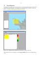
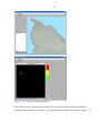
given in Figure L.1 and in (10).
Figure L.1
Ground conductivity map of Norway, from (10). Numbers are given in units of
mS/m.


![[SANTIAGOLITEM.NET]](http://vs1.manualzilla.com/store/data/006051955_1-6793608479d1e718412b318dacd9cbdc-150x150.png)