Download QuickFil User Manual

4XLFN)LO
8VHU0DQXDO
4XLFN)LO
© OMICRON electronics 2002. All rights reserved.
The product information, specifications, and all technical data contained within this manual are not
contractually binding. OMICRON reserves the right to make technical changes without announcement.
OMICRON electronics is not to be held liable for statements and declarations given in this manual. The
user is responsible for every application described in this manual. OMICRON electronics explicitly
exonerates itself from all liability for mistakes in this manual. Copying or reproducing this manual,
wholly or in part, is not permitted without the expressed written consent of OMICRON electronics.
2
7DEOHRI&RQWHQWV
7DEOHRI&RQWHQWV
7DEOHRI&RQWHQWV
,QWURGXFWLRQ 1.1 Structure Of The Manual . . . . . . . . . . . . . . . . . . . . . . . . . . . . . . . . . . . . . .9
1.2 Typefaces . . . . . . . . . . . . . . . . . . . . . . . . . . . . . . . . . . . . . . . . . . . . . . . . .9
1.3 Installing QuickFil . . . . . . . . . . . . . . . . . . . . . . . . . . . . . . . . . . . . . . . . . .10
1.4 Starting QuickFil . . . . . . . . . . . . . . . . . . . . . . . . . . . . . . . . . . . . . . . . . . .13
1.5 Remove QuickFil . . . . . . . . . . . . . . . . . . . . . . . . . . . . . . . . . . . . . . . . . . .13
1.6 Hints for the DOS version . . . . . . . . . . . . . . . . . . . . . . . . . . . . . . . . . . . .13
1.7 Quitting QuickFil . . . . . . . . . . . . . . . . . . . . . . . . . . . . . . . . . . . . . . . . . . .14
3URJUDP,QWURGXFWLRQ 2.1 Features . . . . . . . . . . . . . . . . . . . . . . . . . . . . . . . . . . . . . . . . . . . . . . . . .15
2.2 Program Structure . . . . . . . . . . . . . . . . . . . . . . . . . . . . . . . . . . . . . . . . . .18
2.3 Program Support . . . . . . . . . . . . . . . . . . . . . . . . . . . . . . . . . . . . . . . . . . .19
7XWRULDO
3.1 Starting The Program . . . . . . . . . . . . . . . . . . . . . . . . . . . . . . . . . . . . . . .21
3.2 Specifying The Filter . . . . . . . . . . . . . . . . . . . . . . . . . . . . . . . . . . . . . . . .23
3.3 Designing The Circuit . . . . . . . . . . . . . . . . . . . . . . . . . . . . . . . . . . . . . . .28
3.4 Analyzing Circuits . . . . . . . . . . . . . . . . . . . . . . . . . . . . . . . . . . . . . . . . . .30
2SHUDWLQJ,QVWUXFWLRQV 4.1 Selecting Menu Options . . . . . . . . . . . . . . . . . . . . . . . . . . . . . . . . . . . . .33
4.2 Selecting Options Using The Keyboard. . . . . . . . . . . . . . . . . . . . . . . . . .33
4.3 Selecting Options Using The Mouse . . . . . . . . . . . . . . . . . . . . . . . . . . . .34
4.4 Dialog Fields . . . . . . . . . . . . . . . . . . . . . . . . . . . . . . . . . . . . . . . . . . . . . .35
4.5 Entering Data In Fields . . . . . . . . . . . . . . . . . . . . . . . . . . . . . . . . . . . . . .35
3
4XLFN)LO
4.6 Entering Filenames . . . . . . . . . . . . . . . . . . . . . . . . . . . . . . . . . . . . . . . . .36
4.7 On-Line Help Text . . . . . . . . . . . . . . . . . . . . . . . . . . . . . . . . . . . . . . . . . .37
4.8 Output . . . . . . . . . . . . . . . . . . . . . . . . . . . . . . . . . . . . . . . . . . . . . . . . . . .38
4.9 Graphic Output . . . . . . . . . . . . . . . . . . . . . . . . . . . . . . . . . . . . . . . . . . . .39
4.10 Program Setup . . . . . . . . . . . . . . . . . . . . . . . . . . . . . . . . . . . . . . . . . . . .39
3URJUDP)XQFWLRQV 5.1 Specifications . . . . . . . . . . . . . . . . . . . . . . . . . . . . . . . . . . . . . . . . . . . . .43
5.2 Standard Approximations . . . . . . . . . . . . . . . . . . . . . . . . . . . . . . . . . . . .43
5.3 Bessel Lowpass Approximations. . . . . . . . . . . . . . . . . . . . . . . . . . . . . . .48
5.4 General Amplitude Approximations . . . . . . . . . . . . . . . . . . . . . . . . . . . . .51
5.5 SPECIFICATION Menu (for general amplitude approx.). . . . . . . . . . . . .52
5.6 OPTIMIZATION Menu . . . . . . . . . . . . . . . . . . . . . . . . . . . . . . . . . . . . . . .58
5.7 STOPBAND SPECIFICATION Menu . . . . . . . . . . . . . . . . . . . . . . . . . . .65
5.8 TRANSMISSIONZERO INPUT Menu . . . . . . . . . . . . . . . . . . . . . . . . . . .67
5.9 Example 1: Lowpass Filter . . . . . . . . . . . . . . . . . . . . . . . . . . . . . . . . . . .68
5.10 Example 2: Bandpass Filter. . . . . . . . . . . . . . . . . . . . . . . . . . . . . . . . . . .72
5.11 Group delay . . . . . . . . . . . . . . . . . . . . . . . . . . . . . . . . . . . . . . . . . . . . . . .77
5.12 Group delay specification . . . . . . . . . . . . . . . . . . . . . . . . . . . . . . . . . . . .82
5.13 Group delay transmission zeros . . . . . . . . . . . . . . . . . . . . . . . . . . . . . . .83
5.14 Example for Group delay correction . . . . . . . . . . . . . . . . . . . . . . . . . . . .85
5.15 Circuit Design . . . . . . . . . . . . . . . . . . . . . . . . . . . . . . . . . . . . . . . . . . . . .92
5.16 PASSIVE DESIGN menu . . . . . . . . . . . . . . . . . . . . . . . . . . . . . . . . . . . .92
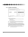
5.17 OUTPUT CIRCUIT Menu . . . . . . . . . . . . . . . . . . . . . . . . . . . . . . . . . . . .94
5.18 SPICE Menu . . . . . . . . . . . . . . . . . . . . . . . . . . . . . . . . . . . . . . . . . . . . . .95
5.19 TOUCHSTONE Menu . . . . . . . . . . . . . . . . . . . . . . . . . . . . . . . . . . . . . . .96
5.20 INPUT CIRCUIT Menu . . . . . . . . . . . . . . . . . . . . . . . . . . . . . . . . . . . . . .97
4
7DEOHRI&RQWHQWV
5.21 Circuits with positive elements . . . . . . . . . . . . . . . . . . . . . . . . . . . . . . . .98
5.22 Computer Circuit . . . . . . . . . . . . . . . . . . . . . . . . . . . . . . . . . . . . . . . . . .103
5.23 Dual Circuit . . . . . . . . . . . . . . . . . . . . . . . . . . . . . . . . . . . . . . . . . . . . . .103
5.24 TERMINATION Menu . . . . . . . . . . . . . . . . . . . . . . . . . . . . . . . . . . . . . .104
5.25 ACCURACY Menu . . . . . . . . . . . . . . . . . . . . . . . . . . . . . . . . . . . . . . . .104
5.26 Sign of the real part of the reflection zeros . . . . . . . . . . . . . . . . . . . . . .105
5.27 MANIPULATION AND ANALYSIS Menu . . . . . . . . . . . . . . . . . . . . . . .107
5.28 DUAL CIRCUIT Menu . . . . . . . . . . . . . . . . . . . . . . . . . . . . . . . . . . . . . .109
5.29 CHANGE VALUES Menu . . . . . . . . . . . . . . . . . . . . . . . . . . . . . . . . . . .110
5.30 NORTON’S TRANSFORMATION Menu . . . . . . . . . . . . . . . . . . . . . . . .111
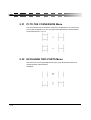
5.31 PI-TO-TEE CONVERSION Menu . . . . . . . . . . . . . . . . . . . . . . . . . . . . .114
5.32 EXCHANGE TWO-PORTS Menu . . . . . . . . . . . . . . . . . . . . . . . . . . . . .114
5.33 SPLIT TWO-PORTS Menu . . . . . . . . . . . . . . . . . . . . . . . . . . . . . . . . . .115
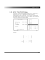
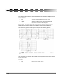
5.34 Example: Bandpass Filter . . . . . . . . . . . . . . . . . . . . . . . . . . . . . . . . . . .116
5.35 Analysis . . . . . . . . . . . . . . . . . . . . . . . . . . . . . . . . . . . . . . . . . . . . . . . . .126
5.36 PROPERTY menu. . . . . . . . . . . . . . . . . . . . . . . . . . . . . . . . . . . . . . . . .130
5.37 REPRESENTATION Menu . . . . . . . . . . . . . . . . . . . . . . . . . . . . . . . . . .131
5.38 TRANSFER menu . . . . . . . . . . . . . . . . . . . . . . . . . . . . . . . . . . . . . . . . .133
5.39 GRAPH_LOAD Menu . . . . . . . . . . . . . . . . . . . . . . . . . . . . . . . . . . . . . .134
5.40 Example: Elliptic Bandpass . . . . . . . . . . . . . . . . . . . . . . . . . . . . . . . . . .135
5.41 Graphics . . . . . . . . . . . . . . . . . . . . . . . . . . . . . . . . . . . . . . . . . . . . . . . .141
5.42 X-Y Menu. . . . . . . . . . . . . . . . . . . . . . . . . . . . . . . . . . . . . . . . . . . . . . . .142
5.43 X-Y PARAMETERS Menu. . . . . . . . . . . . . . . . . . . . . . . . . . . . . . . . . . .143
5.44 X(Y)-SCALE Menu . . . . . . . . . . . . . . . . . . . . . . . . . . . . . . . . . . . . . . . .144
5.45 OUTPUT GRAPHIC Menu . . . . . . . . . . . . . . . . . . . . . . . . . . . . . . . . . .146
5.46 PRINTER OPTIONS Menu . . . . . . . . . . . . . . . . . . . . . . . . . . . . . . . . . .147
5
4XLFN)LO
5.47 X-Y MARKER Menu . . . . . . . . . . . . . . . . . . . . . . . . . . . . . . . . . . . . . . .148
5.48 Output of the roots of the polynomials. . . . . . . . . . . . . . . . . . . . . . . . . .149
5.49 PZ-chart. . . . . . . . . . . . . . . . . . . . . . . . . . . . . . . . . . . . . . . . . . . . . . . . .152
5.50 Macros. . . . . . . . . . . . . . . . . . . . . . . . . . . . . . . . . . . . . . . . . . . . . . . . . .154
5.51 Example: Keystroke Macros . . . . . . . . . . . . . . . . . . . . . . . . . . . . . . . . .157
,663,&(,QWHUIDFH
6.1 QuickFil Output to ISSPICE. . . . . . . . . . . . . . . . . . . . . . . . . . . . . . . . . .165
6.2 Stand-alone Netlist . . . . . . . . . . . . . . . . . . . . . . . . . . . . . . . . . . . . . . . .165
6.3 Subcircuit Netlist . . . . . . . . . . . . . . . . . . . . . . . . . . . . . . . . . . . . . . . . . .167
$SSHQGLFHV
Appendix A - Comparison of Approximations . . . . . . . . . . . . . . . . . .173
Appendix B - Case, Terminating Resistance Ratio . . . . . . . . . . . . . .182
Appendix C - Conventional/Parametric Bandpass Filters . . . . . . . . .191
Appendix D - Design With User Defined Circuits . . . . . . . . . . . . . . .195
Appendix E - Calculation Speed . . . . . . . . . . . . . . . . . . . . . . . . . . . .199
Appendix F - Calculating Component Values . . . . . . . . . . . . . . . . . .200
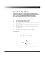
Appendix G - Output Roots . . . . . . . . . . . . . . . . . . . . . . . . . . . . . . . .203
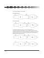
Appendix H - Dual Circuits . . . . . . . . . . . . . . . . . . . . . . . . . . . . . . . .206
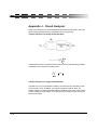
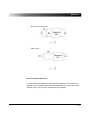
Appendix I - Norton’s Transformation . . . . . . . . . . . . . . . . . . . . . . . .207
Appendix J - Circuit Analysis. . . . . . . . . . . . . . . . . . . . . . . . . . . . . . .212
Appendix K - Circuits with positive elements. . . . . . . . . . . . . . . . . . .215
Appendix L - Group delay correction. . . . . . . . . . . . . . . . . . . . . . . . .217
Appendix M - Key Macro Function . . . . . . . . . . . . . . . . . . . . . . . . . .221
Appendix N - Data Filenames . . . . . . . . . . . . . . . . . . . . . . . . . . . . . .225
Appendix O - Macro File Format (.KDO) . . . . . . . . . . . . . . . . . . . . . .226
Appendix P - Filter Specification Protocol (.SPZ) . . . . . . . . . . . . . . .228
Appendix Q - Polynomial Pole/Zero Protocol (.FDT). . . . . . . . . . . . .229
Appendix R - Circuit Protocol (.SCH) . . . . . . . . . . . . . . . . . . . . . . . .231
Appendix S - Internal Format(.QFT) . . . . . . . . . . . . . . . . . . . . . . . . .232
Appendix T - SPICE Format(.CIR) . . . . . . . . . . . . . . . . . . . . . . . . . .233
Appendix U - Touchstone Format(.CKT). . . . . . . . . . . . . . . . . . . . . .235
Appendix V - Graphics Data Format(.PLT) . . . . . . . . . . . . . . . . . . . .236
Appendix W - Definition File Format (QF.DEF) . . . . . . . . . . . . . . . . .237
Appendix X - Frequently Asked Questions . . . . . . . . . . . . . . . . . . . .247
6
7DEOHRI&RQWHQWV
Appendix Y - Literature . . . . . . . . . . . . . . . . . . . . . . . . . . . . . . . . . . .248
,QGH[
7
4XLFN)LO
8
,QWURGXFWLRQ
,QWURGXFWLRQ
6WUXFWXUH2I7KH0DQXDO
Welcome to 4XLFN)LO
This manual is divided into the following sections:
Chapter 1 “INSTALLATION” - specifies the minimum hardware requirements
and shows how to install the software.
Chapter 2 “PROGRAM INTRODUCTION” - provides you with a short summary
of the program’s features.
Chapter 3 “TUTORIAL” - will acquaint you with the software using a simple
example.
Chapter 4 “OPERATING INSTRUCTIONS” - tells you about the operation of
4XLFN)LO.
Chapter 5 “PROGRAM FUNCTIONS” - provides you with detailed information
on the functions of the program.
Chapter 6 "ISSPICE INTERFACE" - explains the interface to ISSPICE
“APPENDIX” - contains background information on the technical aspects of the
program, instructions for creation of key macros for automatic sequences, and
a list of useful literature.
“INDEX” - allows you to find specific explanations of certain key words.
7\SHIDFHV
In this manual, instructions for communicating with the program through the
keyboard are given as follows:
Examples:
•
10M[↵]
Enter character sequence “10M”, followed by the
ENTER key.
•
[A]
Press “A” to access a menu field.
•
[Ctrl+U]
Press and hold the CTRL key down while pressing
“U”.
9
4XLFN)LO
•
Uppercase letters, followed by a colon, are 4XLFN)LOmenu entries. For
example, SPECIFICATION would refer to the Specification menu.
•
Characters or messages which the program displays on the screen are
shown as follows:
FILTER NOT YET SPECIFIED.
,QVWDOOLQJ4XLFN)LO
4XLFN)LO is a DOS program which can be performed in Windows environment. A
comfortable installation program will reduce the efforts of the user.
There are following versions available:
10
•
CD
The program is on a compact disk (CD ROM)
available for the languages English and German.
Please insert the CD and the installation program
will start automatically. Please choose the
language and follow the further instructions.
•
ZIP-version
This is a ZIP archive for the installation program.
After extracting the ZIP file (using Winzip or some
other extracting program) to some temporary
directory, you can start the installation program by
executing SETUP.EXE. If the installation is
finished, you can remove the temporary directory
and all its files.
•
Executable version
By starting the executable file, a temporary
directory is created and all files are extracted to
that directory. Afterwards, the setup program is
started automatically. If the installation is finished,
this temporary directory is removed.
,QWURGXFWLRQ
+DUGZDUH5HTXLUHPHQWV
Minimum configuration:
•
IBM PC or compatible
•
CGA, HGC, EGA or VGA graphics
Optional:
•
Printer
•
Plotter (HPGL format)
•
Serial interface for output device: only available for Windows 95, Windows
98 and Windows Me
2SHUDWLQJ6\VWHP5HTXLUHPHQWV
•
Windows 95, Windows 98, Windows Me, Windows NT4, Windows 2000
or Windows XP
•
A special DOS version is available on request.
,QVWDOOLQJWKH6RIWZDUH
Before installing 4XLFN)LO:
•
Make a backup copy of the program.
The installation program is an up to date Windows installation program, and is
self explanatory.
After agreeing to the License agreement, you must specify your name and the
name of the company:
11
4XLFN)LO
Afterwards you can specify the directory where the program will be installed:
The default path will be Drive:\Program Files\OMICRON\4XLFN)LO. The default
drive is the drive where the operation system is installed (system drive).
The program will be installed to the specified directory and a short cut to the
desktop will be created. Further, there will be a shortcut to the menu START |
PROGRAMS.
12
,QWURGXFWLRQ
6WDUWLQJ4XLFN)LO
For starting the program 4XLFN)LO, simply click at the icon at the desktop or use
the list in START | PROGRAMS, and choose the program 4XLFN)LO.
5HPRYH4XLFN)LO
Using the menu: START | SETTINGS | CONTROL PANEL | ADD/REMOVE
PROGRAMS, you can remove the program in the standard way for Windows.
If you install a new version of 4XLFN)LO, the old version of the program is removed
automatically.
+LQWVIRUWKH'26YHUVLRQ
Since the basic program is a DOS program, the following hints are for DOS
users.
*UDSKLFV5HODWHG,QVWDOODWLRQ3UREOHPV
Computers with color graphics adapter, but only a monochrome display (e.g.
laptops):
If you are not pleased with the display representation on your screen:
•
Exit the program (by entering [Q], acknowledge with [Y]) and use
extended start command.
•
Type either QF /bw[↵] or QF /lcd[↵].
This switches your computer’s screen to another display mode. If you start the
program properly but still get “junk” on your screen: When the program starts,
4XLFN)LO will automatically check which graphics card is in your computer and set
itself accordingly. However, there are certain circumstances that it may not be
able to identify the card.
7RVROYHWKLVSUREOHP
•
Exit the program.
•
Edit the file QF.DEF in any word processing program (e.g. IsEd, MS
Word, etc.)
•
After the line BEGIN GRAPHICDEFAULTS, change the entry in the line
DISPLAYTYPE to suit your screen.
13
4XLFN)LO
Possible inputs include:
CGAHi
(640x200, mono)
MCGAHi
(640x48, 2-color)
MCGAMed
(640x200, mono)
EGAHi
(640x350, 16 colors (256K))
EGA64Hi
(640x350, 4-color (64K))
EGAMonoHi
(640x350, mono)
HERCMonoHi
(720x348, mono)
ATT400Hi
(640x400, mono)
ATT400Med
(640x200, mono)
)RU([DPSOH
The line, DISPLAYTYPE IBM8514HI, will set the display type to the IBM8514
1024x768 standard.
•
Save the QF.DEF file as an ASCII file.
4XLWWLQJ4XLFN)LO
To quit the 4XLFN)LO program:
14
•
Select Quit, or press Q, or Esc until you are at the 4XLFN)LO main menu.
•
Press Q, while in the 4XLFN)LO menu. Answer yes, to confirm and exit the
program.
3URJUDP,QWURGXFWLRQ
3URJUDP,QWURGXFWLRQ
)HDWXUHV
4XLFN)LOis a CAE software program for specifying, dimensioning and analyzing
passive analog filters. The program offers the following features:
),/7(57<3(6
•
Lowpass
•
Highpass
•
Bandpass
•
Bandstop
$3352;,0$7,216
Standard approximations
•
Elliptic (Cauer filter)
•
Butterworth (potence filter)
•
Chebyshev
•
Inverse Chebyshev
•
Bessel (for lowpass only)
•
Modified Bessel (for lowpass only)
General amplitude approximations
•
Maximally flat
•
Equal ripple
each referring to the passband.
15
4XLFN)LO
&,5&8,7'(6,*1
Passive LC/reactance filters
•
Calculation of filters with topologies suggested by the program, or
•
Design of filters on a modular (piece by piece) basis. With this approach,
the user can synthesize the filter step-by-step. 4XLFN)LOwill provide
selections for each element at each step.
•
Modifications of synthesized circuits (Norton’s transformation etc.)
•
Different terminating resistances and extreme terminations may be
selected.
•
Graphic analysis of the characteristics of the current circuit
•
Interface with the ICAP and Touchstone analysis programs Active RC
filters.
$1$/<6,66(&7,21
Graphical analysis of
•
Transmission characteristics (magnitude, phase response, group delay
etc.)
•
Reflections
•
Impedances
•
Up to four diagrams can be displayed at one time.
•
Linear or logarithmic scaling
•
Auto or manual scaling
•
Waveform Cursor function
•
Output to plotters, printers, or file
$33/,&$7,216
16
•
Design of passive reactance filter circuits
•
Optimization of filter specifications
•
Rapid cost estimating
•
Feasibility studies of different specifications
•
Compare different realization possibilities (approximations, circuit
structures etc.)
3URJUDP,QWURGXFWLRQ
,17(5)$&(
•
Menu-driven
•
Mouse support
•
On-line help information
•
Keystroke macro support
17
4XLFN)LO
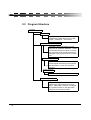
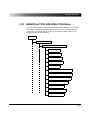
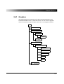
3URJUDP6WUXFWXUH
QuickFil
Specification
Input of filter specifications and
optimization of filter data from “FILTERTYPE:”, “SPECIFIC.:” menu items.
Passive LC / reactance filters
Calculation and optimization of circuit
proposal via “PASSIVE DESIGN:”. Output
circuits with component values. Transfer
the proposed circuit to external analysis
packages. Use proposed circuit or create
one.
Circuits Manipulation
Optimize component values for a design
criteria (equal inductances) using Norton
transformation, Pi-Tee, and Two Port
function.
Circuit Analysis
Graphical display of circuit characteristics.
Analysis of Specification
Graphical display of filter characteristics
based on the characteristic zeros from
“POLY. ANALYSIS:” function. Investigate
the Transfer function or step and pulse
responses of the proposed filter.
18
3URJUDP,QWURGXFWLRQ
3URJUDP6XSSRUW
4XLFN)LO offers interfaces to the following programs:
,663,&(63,&(1(7
Output the filter circuit in an ISSPICE subcircuit format, or as a stand-alone
ISSPICE netlist. When output as a subcircuit, the file created will have the same
format as other SPICE model library files included in the Intusoft ICAPS
package. Netlists may also contain component tolerances for use in the Monte
Carlo statistical yield analysis.
7RXFKVWRQH
Output the filter circuit in a Touchstone netlist format.
All SPICE netlists are in an ASCII format and can be used with virtually any
SPICE program.
19
4XLFN)LO
20
7XWRULDO
7XWRULDO
This chapter will acquaint you with 4XLFN)LO by using a simple example. You will
learn how to:
•
Operate the program
•
Activate the on-line help
•
Enter a filter’s specifications
•
Obtain recommendations for complete filter design
•
Analyze a filter’s characteristics graphically
Hint for mouse users
All examples in this manual are written based on operation from the keyboard.
If you would like to use your mouse in the examples, please read the remarks in
the “Selecting Options Using The Mouse” section.
For this tutorial example, we will design a bandpass filter with the following
specifications:
•
Passband: 87.5 MHz ... 108 MHz
•
Stopband: 0 - 70 MHz and from 140 MHz
•
Stopband attenuation: 45 dB
•
Return loss (matching): 16 dB
Selected approximation: Elliptic filter (Cauer)
6WDUWLQJ7KH3URJUDP
After we have installed 4XLFN)LO, we can start the program by clicking at the icon
on the desktop. Alternatively, we can start the program from the Windows menu
START | PROGRAMS. After a short period, while the program is being
initialized, the Main Menu will be displayed:
21
4XLFN)LO
We are now in the 4XLFN)LO main menu. To get to a defined initial state, we will
reset the program:
•
[O]
Go to the OPTIONS menu. (You can select various
menu functions by entering the appropriate capital
letter. In the letter ‘O’).
•
[R]
Select the program_Reset option.
•
[↵]
Answer to query (Y/N).
•
[Q]
Back to the main menu.
Now we are ready to start the filter design.
22
7XWRULDO
6SHFLI\LQJ7KH)LOWHU
From the main menu, press:
•
[↵]
Change to the FILTERTYPE menu. The screen
will now display the following options:
Initially a Butterworth lowpass is selected. However, we want to calculate a
bandpass filter with an Elliptic approximation. To change to the bandpass filter
type:
•
[↵]
Go to TYPE menu.
•
[B]
Bandpass
Now, we specify the desired approximation.
•
[A]
Change to the APPROXIMATION menu.
•
[E][↵]
Elliptic approximation (Cauer filter)
The screen will show changed settings by highlighting the entries.
23
4XLFN)LO
To use the mouse to activate functions:
•
Just click on the desired settings on the screen.
It is now time to enter the filter specifications.
•
[Q]
Back to the main menu.
•
[S]
Go to the SPECIFICATION menu.
The following screen will appear:
If you’re not clear about any of the terms on the screen, you can call up the online help:
•
[?]
Activates the on-line help.
The following help text will appear:
24
7XWRULDO
The page number in the top right-hand corner, tells us that there are more pages
available on this topic:
•
[N]
Next page
25
4XLFN)LO
Now, we have all the needed information so let’s continue entering our
specifications:
•
[R]
Return to the point in program where the help was
called up.
Now, let’s choose case “c” for equal terminating resistances:
•
[I][C][Enter]
Case “c”
Enter the following specifications:
•
[A]
Lower passband edge frequency
•
87.5M[↓]
Value: 87.5 MHz
Note: please make sure you use the right upper case/lower case scaling units
(e.g. m= milli-, M = mega- etc.) This could also be input as 87.5E6.
•
108M[↓]
Upper passband edge frequency: 108 MHz
•
70M[↵]
Lower stopband edge frequency: 70 MHz
When you confirm the last input, the upper stopband edge frequency will also
appear in the mask (135 MHz). This occurs because with symmetrical bandpass
filters, if any three frequencies are known, the fourth can be calculated. Every
time you enter a value, 4XLFN)LOchecks to see if the entry affects or generates
any other values. We are happy with this value. In fact, it’s less than the value
we wanted! Now let’s enter the required return loss:
•
[F]16[↵]
Return loss: 16 dB
Entering the return loss, automatically gives the passband attenuation:
approximately 0.11 dB.
Next, the stopband attenuation:
•
[G]45[↵]
Stopband loss: 45 dB
Once this input is confirmed, the program automatically calculates the filter
degree and displays it on the screen:
26
7XWRULDO
No doubt you’ve noticed that when the program calculated the degree, it also
revised the stopband attenuation, increasing it to 53.95 dB. With the current
value, this specification still has a margin that can be used to improve other filter
specifications.
We would rather have a better return loss (matching) than a higher stopband
loss. So lets’ try to use this “margin” to improve the return loss.
Degree, stopband attenuation, return loss and passband attenuation vary with
one another, so before we start changing any of these parameters, we need to
know which of the others we can or should change. We can do this by setting
any of these fields to “variable”.
In this case, we want to optimize return loss:
•
[J]
Variable value
•
[F][↵]
Return loss set to “variable”
The position of the arrows, in the right-hand part of the screen, shows us that
changes were made. The three values are set to variable because all three
values are directly linked to one another.
27
4XLFN)LO
Alternatively you can use the mouse:
A change of the variable value can be effected by clicking on the empty space
behind the respective field. 4XLFN)LO then sets the marking to the selected
position. Now let’s enter a new stopband loss which we would prefer - let’s say
50 dB.
•
[G]50[↵]
Stopband attenuation: 50 dB
The screen will now appear as follows:
The return loss has changed and with it, the passband loss.These two factors
are directly connected. (With loss-free filters, the wave (energy), which does not
reach the output, returns to the input).
Now we’re happy with our specifications, so we’ll go on and design the filter:
•
[Q]
Back to the main menu, calculating roots in the
process.
'HVLJQLQJ7KH&LUFXLW
From the main menu type:
•
[D]
Go to the PASSIVE DESIGN menu.
The screen will display the following:
28
7XWRULDO
This screen already shows the circuit topology but not the component values. To
show the values, press:
•
[↵]
Go to the OUTPUT CIRCUIT menu
The program takes a moment while performing the calculations (reactances,
components) and then, displays the circuit on the screen, along with all the
component values.
29
4XLFN)LO
To see the next part of the circuit:
•
[↓]
Scroll through the circuit.
The circuit is displayed with the filter input at the top, the output at the bottom
and the solid line on the left as the ground.
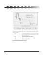
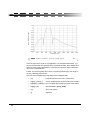
$QDO\]LQJ&LUFXLWV
Let’s take a look at the frequency response of the filter circuit we have designed:
•
[Q]
Back to the PASSIVE DESIGN menu.
•
[M][A]
Go to the CIRCUIT ANALYSIS menu.
•
[X][X][X][↵]200M[↵]
Upper limit X-axis = 200 MHz
•
[O]300[↵]
300 calculated points
•
[↵]
Switch to the waveform plotting mode.
Once the screen display is complete, it will appear as follows:
30
7XWRULDO
Of course, this leaves a lot of room for improvement (limits, scaling etc.). Let’s
get back to our starting point:
•
[Q][Q][Q][Q]
Back to main menu.
In the last step, we will save the filter data and program status for later use:
•
[T][S]example1[↵]
The file is saved under Example1.QF.
This ends the tutorial example!
6800$5<
In this example, you have seen:
•
How to operate the program;
•
How to ask for help;
•
How to specify a filter;
•
How a complete circuit is designed;
•
How to analyze a circuit’s transmission characteristics;
•
How fast 4XLFN)LOactually runs; and
•
How easy it is to design an Elliptic filter.
Further examples are provided in the descriptions of the individual program
functions (Chapter 5).
31
4XLFN)LO
32
2SHUDWLQJ,QVWUXFWLRQV
2SHUDWLQJ,QVWUXFWLRQV
6HOHFWLQJ0HQX2SWLRQV
The 4XLFN)LO menu system is based on a hierarchical tree structure. Selecting a
menu option will take you:
•
to another menu;
•
to an instruction; or
•
to the appropriate data field.
The following key functions are valid throughout the whole program:
[ESC]
Interrupt key. Calculations are also stopped. For
mouse users: The same function can be achieved
by pressing both mouse buttons.
[?]
Invokes the on-line help system.
[Q]
Selects the quit command. Exits from a menu by
maintaining all changes and returns to the
previous menu.
[F1]
Calls up a list of files when the program expects
the entry of a filename.
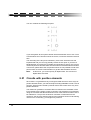
6HOHFWLQJ2SWLRQV8VLQJ7KH.H\ERDUG
You can select any menu option by pressing the first UPPER CASE letter in the
particular menu entry (usually the first letter, but not always).
In most menu functions, each upper case letter occurs only once. If that letter is
pressed, the appropriate command will be immediately executed.
For example:
To move from the main menu to the OPTIONS menu:
33
4XLFN)LO
•
Press [O].
The OPTIONS: menu will be activated.
In menus where the same letter applies to more than one function, the
commands are executed as follows:
•
Successive presses of the capital letter will alternate between the
appropriate functions. To select the desired function, press Enter.
For Example:
You’re in the APPROXIMATION menu and you want to select the Elliptic entry.
Procedure:
•
[E]
Highligth Elliptic
•
[↵]
Confirm selection
The items in the menu can also be selected with the [←], [→].
[Spacebar] or [Backspace] keys and confirmed with [↵].
6HOHFWLQJ2SWLRQV8VLQJ7KH0RXVH
To select menu functions with the mouse:
•
Move the mouse pointer over the desired function.
•
Click the left or right mouse button.
The function you selected will be executed immediately.
34
2SHUDWLQJ,QVWUXFWLRQV
To back up one menu level:
•
Press both the left and right mouse buttons simultaneously.
'LDORJ)LHOGV
In many parts of the program, the dialog with the program takes place through
fields in the screen. Highlighted entries can be selected directly by the user.
Entries in normal video contain additional information and cannot be selected.
The highlighted entries can either be:
•
numbers/texts that can be edited;
•
functions that are executed after being selected; or
•
the valid setting from a range of options.
(QWHULQJ'DWD,Q)LHOGV
Keystrokes Results:
[↵]
End and accept the entry.
[ESC]
End without accepting the entry.
[←], [→]
Move cursor one character to the left/right.
[Ctrl+←], [Ctrl+→]
Move cursor one word to the left/right.
[Home], [End]
Move cursor to the beginning/end of a string of
characters.
[Backspace]
Delete character left of the cursor.
[Ctrl+Backspace]
Delete the whole entry in the input field.
[Ctrl+T]
Delete until the next blank.
[Del]
Delete character at the cursor position.
[Ins]
Switch from “Insert” to “Overwrite” mode.
Additional input options in numerical fields include:
min[↵]
Smallest possible value desired
max[↵]
Highest possible value desired
nn%[↵]
nn% of the presently shown value desired
35
4XLFN)LO
Scaling abbreviations for numbers include:
a
Atto = 1.0E-18
f
Femto = 1.0E-15
p
Pico = 1.0E-12
n
Nano = 1.0E-9
u
Micro = 1.0E-6
m
Milli = 1.0E-3
k
Kilo = 1.0E+3
M
Mega = 1.0E+6
G
Giga = 1.0E+9
T
Tera = 1.0E+12
P
Peta = 1.0E+15
E
Exa = 1.0E+18
(QWHULQJ)LOHQDPHV
Some program functions require a filename to be entered. For these functions,
you can enter filenames in two different ways:
•
Direct entry of a filename in the corresponding field; or
•
Selection of a filename from a list.
Filename extension note: 4XLFN)LO automatically adds the extension the
program expects for the respective data format (see “Data Formats”). If you want
to use another extension, you can enter it along with the filename.
Filename path note: If you enter the filename only, data will be transferred with
the path specified in the OPTIONS menu. If you want to use another path, you
can enter it along with the filename (e.g. a:\test\filter1.ini [↵]).
The scaling abbreviations differ from those used with the ISSPICE analog circuit
simulation program.
Instead of entering a filename, you can call up a list of files and select the one
you want.
36
2SHUDWLQJ,QVWUXFWLRQV
7RVHOHFWDILOHXVLQJWKHNH\ERDUG
•
Press [F1] to call up the list of existing files.
•
Select the file you want by entering the first letter or using the cursor keys.
•
Press [↵] to confirm.
7RVHOHFWDILOHXVLQJWKHPRXVH
•
Place the mouse pointer in the filename field.
•
Press the right mouse button;
•
Then, either press the left mouse button for selection and Enter for
confirmation; or
•
Press the right mouse button for selection and simultaneous confirmation.
2SWLRQVIRUOLVWLQJILOHV
Path names and wildcards such as “?” and “∗” can be used for listing files.
Examples of entries:
∗.∗[F1]
All files (no matter what extension) are listed in the
directory as stated in the OPTIONS menu.
C:\QF\∗.FMT[F1]
All files are listed that have the extension FMT, and
that are contained in the directory, as stated in the
OPTIONS menu.
The first file displayed in the list on the screen is automatically copied to the input
field. After confirming the filename, the data will be transferred.
2Q/LQH+HOS7H[W
To invoke the on-line help text:
•
Press “?”.
You can issue the following instructions from the menu line:
5HVXPH
Return to the 4XLFN)LOmenu screen.
1H[WBSDJH
Display the next help screen.
3UHYLRXVBSDJH
Move back to the previous screen.
37
4XLFN)LO
&RQWHQWV
Open the HELP CONTENTS menu to obtain a list of all the help topics that
you can access.
2XWSXW
4XLFN)LOprovides two types of printer output, text and graphics.
7H[W2XWSXW
This type of output is used in 4XLFN)LOfor printing tables of data, such as
specifications, zero positions, etc.
The printer specifications (type of font, margin, etc.) are set in the OPTIONS
menu, either by entering the respective data field directly (mouse users), or by
the menu items in the PRINTER submenu.
QUICKFIL
OPTIONS
PRINTER
,QWHUIDFHSULQWHUSORWWHU
This item is used for selecting the desired interface for the output device.
,%0FKDUVHW
Determines if the printer is able to print the whole IBM character set (line
symbols).
/LQHVSDJH
Determines the number of lines to begin a new page.
/HIWERUGHU
Determines the left margin in characters.
38
2SHUDWLQJ,QVWUXFWLRQV
3RVW6FULSW
Determines whether your printer is a postscript printer. Relevant only for text
outputs.
&KDUOLQH
Determines the number of characters per line.
,QLW
Offers the option of sending an initialization sequence to your printer. This
sequence is sent to the printer before each printout. Non printable control
characters are provided in the form \nnn, with nnn being a three-digit decimal
number (e.g. ESC = \027). Hint: Don’t enter a sequence if you have a
postscript printer.
)RUH[DPSOH
Control sequence for the HP laser printer IID for 10 pt Courier font is:
\027(10U\027(s0p12.00h10.0u0s0b3T
*UDSKLF2XWSXW
This type of output is used in 4XLFN)LO for printouts of the filter analysis results.
As different output formats are required for the individual printers, 4XLFN)LOfirst
“translates” the respective graphics data into the printer language, and then
transmits the data through the predefined interface. The program contains its
own conversion software for this purpose.
The printer settings (type of printer, desired size of the drawing, etc.) are made
in the PRINTER OPTIONS menu (from the menu OUTPUT GRAPHIC, select in
the graphics section). For more details, please refer to the “Output Graphic”
section.
3URJUDP6HWXS
4XLFN)LOallows you to set certain program options. The program automatically
switches to these settings at start-up. The respective settings are made in the
OPTIONS menu. For settings activated from the keyboard (without mouse
support), there are additional submenus.
39
4XLFN)LO
QUICKFIL
OPTIONS
PRINTER
INTERFACE
For example, the following settings can be programmed:
•
The DOS path where data is searched/saved. (If no alternate path has
been added to the filename.)
•
Interface parameters for the peripheral output devices (printer, plotters,
etc.).
•
The type of decimal point used (./,).
•
Number groupings (yes/no).
The OPTIONS menu also tells how much memory is left and gives the precise
version number of this program.
The entries in the OPTIONS menu are:
'ULYH3DWK
This entry contains the path to the DOS directory where data files will be
saved. (If an alternate path was not provided when the filename was
entered.)
,QWHUIDFH3ULQWHU
This sets the printer interface parameters.
,QWHUIDFH3ORWWHU
This sets the plotter interface parameters.
40
2SHUDWLQJ,QVWUXFWLRQV
If you would like to print your diagrams through another interface (e.g. IEC
interface), you can proceed as follows:
•
Instead of printing the output on a printer, save the graphics data to a file
using the HPGL format. (menu item File in the OUTPUT GRAPHIC menu)
•
Exit from 4XLFN)LOand plot the graphics from the DOS prompt (copy the
contents of the file to the respective plotter port).
'HFLPDOVLJQ
Determines whether the “.” or “,” is used as the decimal point.
*URXSLQJ
Determines whether “longer” numbers in fixed point displays are to be
divided into groups of three for clarity. When selecting the groups of
numbers, the decimal separating point is used that is inverse to the selected
decimal sign.
3ULQWHU6HWXS
Determines the printer settings for text output.
3DUDPHWHUV2I6HULDO3RUWV
Determines the parameters for the serial interface(s) COM1/ COM2:. If the
mouse is installed on one of these ports, the settings cannot be altered.
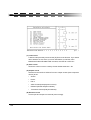
The following parameters can be selected:
Baud rate: 110, 150, 300, 600, 1200, 2400, 4800, 9600
Parity: No, Even, Odd
Data bits: 7, 8
Stop bits: 1, 2
1RWH
Since the 4XLFN)LO is a DOS Program and it will communicate with
the serial ports directly, you will have problems in Windows,
especially for Windows NT, Windows 2000 and Windows XP. In
Windows, all serial ports are normally switched off.
4XLFN)LOautomatically determines which ports are present in the computer.
The OPTIONS menu also contains the Prog_Reset menu item through which
the program can be reset to a defined initial state.
You should be absolutely sure when activating this function because all
previously entered information will be lost!
41
4XLFN)LO
1RWH
42
The saving/loading of program status (program setups with filter
data, graphic parameter, etc.) is possible through the TRANSFER
menu item in the main menu.
3URJUDP)XQFWLRQV
3URJUDP)XQFWLRQV
6SHFLILFDWLRQV
The desired type of filter and the approximation are selected in the FILTERTYPE
menu. The FILTERTYPE menu is selected from the main menu.
QUICKFIL
FILTERTYPE
TYPE
APPROXIMATION
After determining the desired filter type, various filter characteristics are entered
in the SPECIFICATION menu.
6WDQGDUG$SSUR[LPDWLRQV
For standard filter approximations(Butterworth, Chebychev, inverse Chebychev,
Elliptic), specifications are made in the SPECIFICATION menu.
QUICKFIL
SPECIFICATION
43
4XLFN)LO
Depending on the filter type, the following menu will be shown:
/RZSDVVRUKLJKSDVVILOWHUV
%DQGSDVVRUEDQGVWRSILOWHUV
Selections are made by pressing the appropriate key letter which corresponds
to the field on the screen that you wish to edit. Depending on the filter type, only
the relevant settings will be available for entry.
44
3URJUDP)XQFWLRQV
Following menu items are available:
/RZHUSDVVEDQGHGJHIUHTXHQF\
The (lower) frequency at which the loss reaches the specified passband loss
(see diagram at the end of this section).
8SSHUSDVVEDQGHGJHIUHTXHQF\
The upper frequency at which the loss reaches the specified passband loss
(for bandpass and bandstop only, see diagram at the end of this section).
/RZHUVWRSEDQGHGJHIUHTXHQF\
The (lower) frequency at which the loss reaches the specified stopband loss
(see diagram at the end of this section).
8SSHUVWRSEDQGHGJHIUHTXHQF\
The upper frequency at which the loss reaches the specified stopband loss
(for bandpass and bandstop only, see diagram at the end of this section).
As an alternative to the individual edge frequency values, 4XLFN)LO also allows
you to enter data in the bandwidth/relative display. (Only for the standard
approximations of bandpass or bandstop filters using symmetrical responses.)
Change through the menu items EDQGZLGWKUHSUH6. and reL.bandwidthrepres.;
with IUHT8HQF\UHSUHV. You can return to the frequency display.
The center frequency, stated in the bandwidth display, refers to the geometrical
center with reference to the logarithmically applied frequency axis.
3DVVEDQGEDQGHGJHORVV
Maximum loss in the passband (see diagram at the end of this section).
3DVVEDQGEDQGHGJHUHWXUQORVV
This entry is only relevant to passive LC filters (reactance filters). The return
loss is the reflection factor in "dB" Format.
Examples:
•
r=1
return loss = 0 dB
•
r = 0.1
return loss = 20dB
Return loss is directly coupled to passband attenuation.
45
4XLFN)LO
3DVVEDQGUHIOHFWLRQIDFWRU
Ratio of the amount of the reflected signal to the amount of the input signal,
in percent. The reflection factor can be calculated from the input impedance,
directly (see appendix J).
The reflection factor is directly coupled to the passband and return loss.
6WRSEDQGORVV
Minimum loss in the stopband (see diagram at the end of this section).
)LOWHUGHJUHH
The number of attenuation peaks of the filter circuit (peaks where s -> infinity
included). The degree of a filter is an indication of the number of components
required.
&DVH
For even degree lowpass and highpass filters, and for bandpass and
bandstop filters whose degree is divisible by four, there are frequency
transformations available which are represented by cases.
D Case "a" is available for Invers Chebychev and for Elliptical filters. Case "a"
means that no frequency transformation is used. Invers Chebychev and
Elliptical filters are not realizable if it’s an even degree lowpass/highpass, or
a bandpass or bandstop filter whose degree is divisible by four, since there
is no transmission zero at zero and no transmission zero at infinity.
Therefore, no passive ladder filter can be realized. By using a frequency
transformation, you can get a realizable filter.
E Case "b" is available for Chebychev, Invers Chebychev and for Elliptical
filters. Case "b" guarantees that there is at least one transmission zero at
zero or at infinity. For Chebychev filters case "b" is the standard not
transformed filter. For Invers Chebychev and for Elliptical, the largest
transmission zero of the even degree prototype lowpass is transformed to
infinity. For even degree filters and Chebychev or Elliptical approximation,
input and output resistance are different.
F Case "c" is available for Chebychev and for Elliptical filters. Case "c"
guarantees that there is at least one transmission zero at zero or at infinity,
and the input and output resistance of the passive filter are equal. The largest
transmission zero of the even degree prototype lowpass is transformed to
infinity, and the lowest reflection zero is transformed to zero.
For more information, see the section “Case, terminating resistance ratio”.
46
3URJUDP)XQFWLRQV
9DULDEOHYDOXH
You can use this field to specify which characteristic of a filter 4XLFN)LO can,
or should change, if any of the screen inputs changes (e.g. during editing the
specifications). The variable value is shown by an arrow at the end of the
editing field.
The screen contains the following additional information:
G%HGJHIUHTXHQF\
The frequency at which the passband loss reaches -3 dB of its maximum
value (precisely: 3.0103 dB). This value is calculated for the user as further
information. It cannot be changed like parameters of input fields directly.
)LOWHUTXDOLW\
Maximum pole quality of the zeros of polynomial e(s). This value is calculated
for the user as further information. It cannot be changed like parameters of
input fields directly. For passive LC-filters, the inductors quality should be
designed with a factor of 3 to 5 higher than the stated filter quality when
realizing the filter.
The following options are also available:
1HZ
Deletes all data contained on the screen in preparation for new input.
F2PPHQW
4XLFN)LOautomatically labels all outputs (roots, circuits, graphs) with
comments that you can enter via this option.
IL/H
Saves the entered filter specifications in a file. The default extension is .SPZ.
For more information on this data format, see the section on “Filter
Specification Protocol”.
For more details, please refer to the section on “Output”.
3ULQWHU
Prints the filter specifications.
47
4XLFN)LO
You can specify the filter demands by simply editing the input fields (pressing
the letter, defined at the beginning), using the cursor key to skip to the next input
field, or by simply using the mouse. If all input fields are specified, you can
change the values of the input fields. Since all possible specifications are
dependent on each other, every change will produce changes to other fields.
The variable field is shown by an arrow at the end of the field. You can specify
the variable field which should change if you edit one input field by the special
menu item 9DULDEOHYDOXHor by simply clicking on the field where you would
like to have the "variable arrow".
The possibility to adjust the filter parameters to the users demands is one of the
main and unique features of 4XLFN)LO.
%HVVHO/RZSDVV$SSUR[LPDWLRQV
Bessel filters are lowpass filters which have a flat group delay response. Since
the transformations from lowpass to highpass, bandpass and bandstop filters do
not preserve the flat group delay response, only lowpass filters make sense.
There are two approximations available: Bessel and Modified Bessel.
48
3URJUDP)XQFWLRQV
Selections are made by pressing the appropriate key letter corresponding to the
field on the screen that you would like to edit. Depending on the type of filter,
only the relevant settings will be available for entry.
Following menu items are available:
G%HGJHIUHTXHQF\
The frequency at which the loss reaches -3 dB of its maximum value
(precisely: 3.0103 dB). Here you can specify a kind of cut off frequency of the
lowpass filter.
*URXSGHOD\DW]HUR
The group delay at the frequency zero. Here, you can specify the group delay
at the frequency zero. The group delay is maximally flat and will decrease
with increasing frequency.
6WRSEDQGHGJHIUHTXHQF\
The frequency at which the loss reaches the specified stopband loss.
49
4XLFN)LO
6WRSEDQGORVV
Minimum loss in the stopband.
)LOWHUGHJUHH
The number of attenuation peaks of the filter circuit (peaks where s -> infinity
included). The degree of a filter is an indication of the number of components
required.
&DVH
For Modified Bessel approximations and even degree filters, we differentiate
between various “cases”.
D This is the basic approximation without any frequency transformation. Since
even degree Modified Bessel lowpass filters have no transmission zeros at
infinity, the required transmission characteristic cannot be realized by a
passive ladder filter. This feature is included for analysis possibilities.
E The largest transmission zero of the Modified Bessel lowpass of even degree
is transformed to infinity. Therefore, there is at least one transmission zero at
infinity and the transfer function can be realized by a passive ladder circuit.
For more information, see the section “Case, terminating resistance ratio”.
9DULDEOHYDOXH
You can use this field to specify which characteristic of a filter 4XLFN)LO can,
or should change if any of the screen inputs change (e.g. during editing the
specifications). The variable value is shown by an arrow at the end of the
editing field.
The screen contains the following additional information:
)LOWHUTXDOLW\
Maximum pole quality of the zeros of polynomial e(s). This value is calculated
for the user as a further information. It cannot be changed like parameters of
input fields directly. For passive LC-filters, the inductors quality should be
designed with a factor of 3 to 5 higher than the stated filter quality when
realizing the filter.
)UHTXHQF\DWJURXSGHOD\
The frequency at which the group delay will be reduced to 90% of the delay
at zero frequency. This item is only for information of the user so he can
estimate the bandwidth of the flat delay.
50
3URJUDP)XQFWLRQV
The following options are also available:
1HZ
Deletes all data contained on the screen in preparation for new input.
F2PPHQW
4XLFN)LOautomatically labels all outputs (roots, circuits, graphs) with
comments that you can enter via this option.
IL/H
Saves the entered filter specifications in a file. The default extension is .SPZ.
For more information on this data format, see the section on “Filter
Specification Protocol”.
For more details, please refer to the section on “Output”.
3ULQWHU
Prints the filter specifications.
*HQHUDO$PSOLWXGH$SSUR[LPDWLRQV
When selecting a general amplitude approximation (equal ripple or maximally
flat), further specifications for the filter are made in the SPECIFICATION menu
and its respective submenus:
QUICKFIL
SPECIFICATION
OPTIMIZATION
STOPBAND SPECIFICATION
TRANSMISSIONZERO INPUT
TRANSMISSIONZERO INPUT
51
4XLFN)LO
63(&,),&$7,210HQXIRUJHQHUDODPSOLWXGH
DSSUR[
Depending on the type of the filter, the following menu will be shown:
/RZSDVVRUKLJKSDVVILOWHUV
%DQGSDVVILOWHUV
52
3URJUDP)XQFWLRQV
%DQGVWRSILOWHUV
Once you have entered the filter type and the approximation (FILTERTYPE
menu), use this menu to specify the filter. Selecting one of the letters in the menu
will take you to the corresponding field on the screen. The program will only
allow you to enter the characteristics that apply to the selected filter type. The
available characteristics are:
/RZHUSDVVEDQGHGJHIUHTXHQF\
The (lower) frequency at which the loss reaches the specified passband loss.
8SSHUSDVVEDQGHGJHIUHTXHQF\
The upper frequency at which the loss reaches the specified passband loss
(only for Bandpass and Bandstop filters).
1RWH
After completing the specification for bandstop filters, it is only
possible to change one of the edge frequencies. When one edge
frequency is changed, the other edge frequency is automatically
changed while the center frequency is kept constant. This is due to
the fact that bandstop filters are always symmetrical.
1RWH
Ifyou would like to specify a very narrow band bandpass or
bandstop filters, there are limits in the program to avoid wrong data
and numerical problems. But if you need this very narrow band
filters, you can change that limit in the 4XLFN)LODefaults File
(QF.DEF) (see Appendix)
53
4XLFN)LO
3DUDPHWHU
This parameter is only available for parametric bandpass filters. In bandpass
filters, you have to distinguish between conventional or parametric types of
responses (change in Parametric/Conventional menu item). If the parametric
form is selected, the screen will contain an input field for the parameter. This
gives you more freedom for dimensioning. (For more details please refer to
the section “Parametric Bandpass Filter” and the explanations in the
Appendix “Conventional/Parametric Bandpass Filters”).
By selecting the 'HIDXOWSDUDP menu item you may accept the default
parameter provided by the program. It is the geometric mean of the lower and
upper passband edge frequencies.
A negative parameter value can also be entered. However, it will only have
an influence on the structure of the circuit in parametric filters of odd degree.
Passband bandedge loss
3DVVEDQGEDQGHGJHORVV
Maximum allowable loss in passband.
3DVVEDQGEDQGHGJHUHWXUQORVV
This entry is relevant only to passive LC filters (reactance filters). The return
loss is the reflection factor in "dB" Format.
Examples:
•
r=1
return loss = 0 dB
•
r = 0.1
return loss = 20dB
3DVVEDQGUHIOHFWLRQIDFWRU
Ratio of the amount of the reflected signal to the amount of the input signal
in percent. The reflection factor can be calculated from the input impedance,
directly (see appendix J).
The reflection factor is directly coupled to the passband and return loss.
7UDQVP]HURVDW]HURLQILQLW\%DQGVWRS7UDQVP]HURSDLUVDWFHQWHU
The number of transmission zeros desired can be entered here in the
“extreme” frequencies, depending on the filter type. The entries are
understood as fixed transmission zeros.
Default settings:
Lowpass: 1 transmission zero at infinity
Highpass: 1 transmission zero at zero
54
3URJUDP)XQFWLRQV
Bandpass: 1 transmission zero at zero and one at infinity
Bandstop: 1 pair of transmission zeros at center frequency
When entering the transmission zeros at zero in conventional bandpass
filters, the number of transmission zeros at infinity is corrected in such a way
that the filter always has an even degree, since odd degree conventional
bandpass filters don’t exist. Parametric bandpass filters require at least one
transmission zero at zero and one at infinity.
How the number of fixed transmission zeros can be determined in a given
circuit is discussed in the “Design With User-DefinedCircuits” section.
1RWH
If a sufficient number of transmission zeros is set at zero and/or
infinity, for achieving the minimum losses (with no fixed or variable
transmission zeros in the finite stopband), you will receive a filter
with a monotonic loss curve in the stopband.
/RVVDW]HURLQILQLW\
This parameter is only available for equal ripple approximation but not for
bandpass filters. For lowpass and highpass filters, the degree of the filter has
to be even. For bandstop filters the degree is divisible by four. You can adjust
the resistance ratio of the ladder circuit by this parameter. If you would like to
have the best filter for the given limits of loss in the passband, please choose
the same value as you took for the passband bandedge loss. If it is important
to have a passive ladder filter which has the same terminating resistance at
the input and at the output, please take the value 0 dB.
For more details please refer to the section on “Equal Ripple
Approximations”.
5HVLVWDQFHUDWLR
This parameter is only available for equal ripple approximation but not for
bandpass filters. For lowpass and highpass filters, the degree of the filter has
to be even. For bandstop filters the degree is divisible by four. Here you can
explicitly adjust the resistance ratio of the passive ladder circuit. The
"resistance ratio" is directly coupled with the "loss at zero/infinity".
For more details please refer to the section on “Equal Ripple
Approximations”.
55
4XLFN)LO
For a better overview of the overall filter specifications, the following data is also
available:
)L[HGWUDQVP]HURSDLUV
This entry informs you about how many fixed pairs of transmission zeros
(these are notch frequencies) you have provided with finite frequencies
(menu item IL;WUDQV]HURV).
9DUWUDQVP]HURSDLUV
This entry informs you how many variable pairs of transmission zeros are
within the finite stopband. If the position of the variable pairs of transmission
zeros was optimized by 4XLFN)LO(OPTIMIZATION menu), the remark opt.
can be seen in this screen (field directly behind their number).
1RWH
4XLFN)LO exclusively deals with symmetrical bandstops. The
number of pairs of transmission zeros is always even in the finite
frequency range because there is no theory available for bandstop
filters, which are not symmetrical and can be realized by ladder
filters.
)LOWHUGHJUHH
The degree is the number of attenuation peaks of the circuit (the
transmisssion zeros at zero and at infinity are also counted). Beware: Pairs
of transmission zeros always mean two transmission zeros. The degree of a
filter is an indication for the number of components required. Maximum
degree: 50
The entry in this screen depends on the settings in the OPTIMIZATION: menu.
Note: In conventional bandpass and bandstop filters the degree must be even.
G%HGJHIUHTXHQF\
Provides the setting at which frequency/frequencies the loss passes the 3dB
edge (precisely: 3.0103 dB).
1RWH
The calculation of the 3dB limits after changing the data requires a
certain amount of time. In higher degrees, however, waiting periods
can become quite lengthy. Therefore, it is also possible to turn off
the calculation of the 3dB limits (For more details see the Appendix
on the 4XLFN)LO Defaults File (QF.DEF)). The calculation will take
place when the filter quality, if desired, is to be calculated.
)LOWHUTXDOLW\
Maximum pole quality of the zeros of polynomial e(s). This value is calculated
for the user as a further information. It cannot be changed like parameters of
56
3URJUDP)XQFWLRQV
input fields directly. For passive LC-filters the inductors quality should be
designed with a factor of 3 to 5 higher than the stated filter quality when
realizing the filter.
1RWH
The filter quality is only calculated if the TXDOLW< menu item is
selected. The calculation of the filter quality requires the calculation
of the whole filter characteristics and will take time. If you leave the
specification menu and enter it again, the calculation of the filter
characteristics is calculated too and you can see the filter quality on
the screen.
6WRSEDQGRSW
Activates the OPTIMIZATION menu. Here, the required minimum loss curve
in the stopband (entry of the tolerance scheme) is specified and the
optimization of the position of the transmission zeros lying in the finite
stopband is performed. For further details please refer to OPTIMIZATION:
Menu section.
IL;WUDQV]HURV
Activates the TRANSMISSIONZERO INPUT submenu for entering the
position of fixed transmission zeros. These will also be considered when
optimizing the position of the variable transmission zeros in the
OPTIMIZATION menu. A practical application would be the suppression of
pilot frequencies. For further details, please refer to the
“TRANSMISSONZERO INPUT” section.
F2PPHQW
4XLFN)LO automatically labels all outputs (roots, circuits, diagrams) with
comments which you can enter via this option, e.g. If you specify a project
number, you will always know which printout belongs to which project.
1HZ
Clears the screen for the specification of a new filter.
IL/H
Saves the filter specifications in a file. Default extension: .SPZ
3ULQWHU
Sends the filter specifications to a printer.
57
4XLFN)LO
237,0,=$7,210HQX
In this menu you can enter the a curve of the minimum losses in the stopband
(tolerance scheme). You can also optimize the number and position of the
transmission zeros which are arranged within the stopband, allowing the
required stopband loss curve to be reached (modified Remez algorithm).
*HQHUDO6HTXHQFH2I(QWULHV
The “classical” sequence of entries in this program takes place in the following
order:
(QWU\2I7KH7ROHUDQFH6FKHPH
From the OPTIMIZATION menu...
For lowpass, highpass and bandstop filters, use the sTopband-specification
menu item.
For bandpass filters, use the Lower/Upper_stopband-spec menu item.
This brings you to the STOPBAND SPECIFICATION menu.
The tolerance scheme has a stepped profile. In the case of an individual curve,
the tolerance scheme can be approximated in small steps. The tolerance
scheme serves as a unilateral edge, i.e. the optimization tries, through the
optimal arrangement of the positions of the transmission zeros, to move the real
loss curve at each point as far away as possible from the tolerance scheme.
58
3URJUDP)XQFWLRQV
The tolerance scheme is only valid in the stopband and must be defined before
the optimization can proceed. In bandpass filters, you have to distinguish
between the upper and lower stopbands. If no particular requirements are set on
one of the two bands, the optimization can only be carried out with one specified
stopband (e.g. only the lower tolerance scheme).
1RWH
A maximum of fifty steps is allowed for the tolerance scheme.
4XLFN)LO does not care about the filter’s loss outside of the stopband frequency
range (transitional range between the stopband and the passband) and this
range will not be taken into account for determining the loss reserve.
([SODQDWLRQRIWKHWHUPV
Example bandpass:
Transitional Ranges
59
4XLFN)LO
Example bandstop:
Transitional Ranges
The specified tolerance scheme is automatically saved. It can be included in the
graphical display of the loss curve in dB, along with the actual filter response.
For more details, please refer to “Circuit Analysis” section.
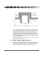
$XWRPDWLF,QLWLDOL]DWLRQ2I7KH9DULDEOHWUDQVPLVVLRQ]HURV
When exiting the STOPBAND SPECIFICATION menu, 4XLFN)LO will make a
proposal for the required number and position of the variable transmission zeros
that will achieve the required stopband loss curve in the respective frequency
range. These values are the initial values that will be used for the subsequent
optimization process.
1RWH
The evaluation does not take into account the number of already
specified fixed transmission zeros at zero, infinity, and the center
frequency (bandstop filters). It also does not take into account the
pairs of fixed transmission zeros in the finite frequency range already
entered by the user.
More details on how 4XLFN)LO establishes the number and position of the
transmission zeros for the initial values of the optimization can be found in the
“Determination Of Variable Transmission zero Pairs” section.
60
3URJUDP)XQFWLRQV
&KDQJLQJWKH1XPEHURI3URSRVHG7UDQVPLVVLRQ=HURV
The determined number of variable transmission zeros will be stated in the
OPTIMIZATION screen. This value can be increased or decreased, as desired,
before the optimization is started. A new initialization is made whenever the
number of transmission zeros is changed in this manner.
1RWH
From this menu it is also possible to change the number of
transmission zeros at zero, infinity, or the center frequency (in
bandstop filters). When making these changes, the entry in the
SPECIFICATION menu is also altered. If no variable transmission
zeros are entered, the loss reserve can, nevertheless, be determined
by selecting 2SWLPL]DWLRQor ,WHUDWLRQ. If there are also no fixed
transmission zeros, the loss curve in the stopband is monotonic.
9LHZLQJDQG(GLWLQJ9DULDEOH7UDQVPLVVLRQ=HURV
For special cases, 4XLFN)LO allows you to preset the individual positions of the
variable transmission zeros in the stopband, or to modify the result of the
program’s initialization. In order to perform these functions, enter the
TRANSMISSIONZERO INPUTmenu through the
9DULDEOHBWUDQVPLVVLRQ]HURV menu function. 4XLFN)LO presumes that the user
would like to pursue a particular goal, for example, changing the initial condition
for the optimization. Hence, there is no automatic initialization of the
transmission zeros afterwards. For more details on the TRANSMISSIONZERO
INPUT menu, please refer to the “Transmissionzero Input” section.
1RWH
Variable transmission zeros can only be positioned within the range of
the tolerance scheme.
2SWLPL]DWLRQRIWKH7UDQVPLVVLRQ=HURV
After having finished determining the number and the initial positions of the
variable transmission zeros in the stopband, the optimization can be carried out
by the program. The optimization is started by the OPTIMIZATIONmenu
function.
The variable transmission zeros lead to "arcs” in the loss curve. Each of these
“arcs” comprises a minimum distance to the predetermined tolerance scheme
(in most cases the “cusp point” of the arc). During the optimization the variable
transmission zeros are moved in iterative steps in the stopband in such a way
that all the minimum distances have the same distance and that the difference
between the highest and the lowest minimal distance converges towards zero.
The program proposes a difference of 0.1 dB as the stop limit for the
61
4XLFN)LO
optimization. However, this value can be changed individually, if desired. If after
concluding the optimization, better values can be achieved, further single
iterations can be carried out through the Iteration menu item.
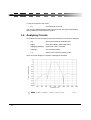
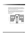
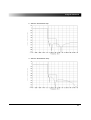
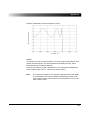
Example for a lowpass:
1. Arrangement after the initialization:
62
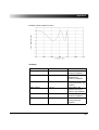
3URJUDP)XQFWLRQV
2. After the first iteration step:
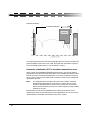
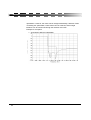
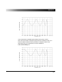
3. After the third iteration step:
63
4XLFN)LO
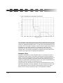
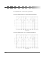
4. After completing the optimization (6 iterations):
The optimization may lead to a loss reserve that is greater than required. If this
is the case, then either the degree of the filter can be reduced by decreasing the
number of variable transmission zeros, or a reduction in the passband loss can
be made. One can usually increase the return loss by the approximate value of
the reserve. In both cases, however, it is necessary to carry out a new
optimization and check whether the change makes the loss fall below the
required value. This would be indicated by a negative sign in the value of the
minimum loss reserve after completing the optimization.
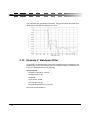
%DQGSDVVILOWHUV
During the optimization of certain bandpass filters, it is possible for a pair of
transmission zeros to assume real values instead of the required imaginary
values. You can recognize this by the number of pairs of transmisssion zeros in
the upper and lower stopband. The total of which does not result in the set
number of variable pairs of transmission zeros. In any case, the optimization can
maximally yield one real pair of transmission zeros.
However, there are cases where such real pairs of transmission zeros occur
during the optimization and then disappear. It is also possible that such a real
pair of transmission zeros is required for the optimum solution. But, with a
passive circuit of the form presently used, it is not possible to realize it.
64
3URJUDP)XQFWLRQV
In order to remedy this problem, you can displace the real pair of transmission
zeros to zero or infinity, or split them to zero and infinity. This solution is
successively requested by 4XLFN)LO in such a case. If you do not agree with any
proposal, the optimization is ignored and 4XLFN)LO will use the values provided
before the optimization as the variable transmission zeros.
It is also possible to make only one iteration. Again, the same problems with real
pairs of transmission zeros might occur. Variable transmission zeros can also be
moved back and forth between the upper and lower stopband during the
optimization.
6723%$1'63(&,),&$7,210HQX
In this menu, the stopband settings for general equal ripple and maximally flat
approximations are entered.
)LUVWHQWU\
The edge frequencies of the stopband specifications are numbered
consecutively and listed according to frequency.
Proceed as follows for the first entry:
•
Select the Add menu item.
•
Confirm the proposed number in the range.
The following steps will depend on the type of filter being synthesized:
/RZSDVV
•
Enter the frequency from which a certain stopband loss is to be achieved.
•
Then, enter the desired loss value. The range ends at infinity if no further
range is specified afterwards or at the beginning of the next range.
+LJKSDVV
•
Enter the frequency up to which a specific stopband loss is desired.
•
Then, enter the desired loss value. The range begins at zero, if a range
was not entered before or from the end of a previous range.
%DQGSDVV
Lower stopband: like highpass
Upper stopband: like lowpass
65
4XLFN)LO
%DQGVWRS
•
Enter the frequency from which a specific loss is to be reached, and then
the frequency up from which this is desired.
•
Then, enter the desired loss value. In the next range, 4XLFN)LO will use the
upper edge frequency of the last range as the “initial frequency” and
expects the entry of the frequency up to which the new loss is set. Then,
enter the loss value for this range.
1RWH
The number of frequency ranges that can be entered for lowpass,
highpass and bandpass filters is 50 (bandstop 49).
&KDQJHVWRSEDQGVHWWLQJV
To change individual values:
•
Click on the fields in the screen with your mouse (scroll with the mouse
pointer on the screen edge if the table is longer);
or
•
Select the Edit menu item, then select the desired value with up and down
arrows and make the pertinent changes.
,QVHUWLRQRIDQHZUDQJH
A range with another loss can also be “inserted” afterwards by entering the
number of the range within which a new range is to be specified. 4XLFN)LO will
then allow you to enter frequency values which lie within the range that has
already been specified.
'HOHWH
Deletes individual ranges by entering the respective number.
1HZ
Deletes all stopband settings shown on the screen.
When exiting the menu, the transmission zeros are initialized first, i.e. 4XLFN)LO
makes a first proposal for the number and positions of the variable transmission
in the stopband. This serves as the initial setting for the following optimization.
For more details please refer to the OPTIMIZATION menu section.
66
3URJUDP)XQFWLRQV
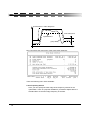
75$160,66,21=(52,13870HQX
This menu is used for entering and changing fixed, as well as, variable
transmission zeros.
In lowpass, highpass and bandstop filters, the entered transmission zeros are
sorted in two columns with rising frequencies. In bandpass filters, the
transmission zeros of the lower stopband are entered in the left column and the
transmission zeros of the upper stopband in the right column.
Bandpass filters: If there is insufficient space in the column for all of the stopband
transmission zeros, the sorting arrangement according to the upper and lower
stopband is dropped. The frequencies will also be sorted according to rising
frequencies in the two columns. For optical separation, a blank line is inserted
between the transmission zeros of the upper and lower stopband.
Bandstop filters: In bandstop filters, two transmission zeros are always treated
symmetrically to the center frequency. It is only possible to have an even
number of pairs of transmission zeros. When making entries or changes, the
complementary frequency belonging to a specific transmission zero is also
updated automatically.
$GG
Used to add a transmission zero to the existing list.
(GLW
To edit a specific field:
•
Select the field with the up or down arrows and enter the data.
•
Then, confirm the entry with [↵].
Under certain circumstances, the table might be sorted again (in accordance
with rising frequencies).
1HZ
Deletes all entries in preparation for a new filter.
67
4XLFN)LO
7RGHOHWHLQGLYLGXDOWUDQVPLVVLRQ]HURIUHTXHQFLHV
•
Switch to the editing mode using Edit menu item.
•
Select the transmission zero to be deleted using the down arrow.
•
Delete the entry in the field using the control backspace key combination.
•
Then, confirm the entry with [↵].
•
Mouse users: Instead of performing the first two items, just click on the
respective field with the mouse pointer.
([DPSOH/RZSDVV)LOWHU
For this filter, we desire a loss curve in the passband with equal ripple. The
stopband will be optimized to a tolerance scheme with stepped profile.
6SHFLILFDWLRQV
Passband edge frequency: 1 kHz
Maximum allowed ripple in dB: 1 dB
Stopband loss:
from 1.05 kHz: 45 dB
from 1.6 kHz: 75 dB
From the main menu proceed as follows:
68
•
[↵]
Change to the FILTERTYPE menu.
•
[↵]
Change to the TYPE submenu.
•
[↵]
Set the type of filter to lowpass.
•
[A]
Change to the APPROXIMATION submenu.
•
[↵]
Set the equal ripple approximation.
3URJUDP)XQFWLRQV
The following entries are selected in the screen:
Now select:
•
[Q]
Return to main menu (If any other requirements
were entered, confirm the request with [Y]).
•
[S][N]
Change to the SPECIFICATION menu and
prepare for a new filter.
•
[↵]1k[↓]
Passband edge frequency: 1 kHz
•
1[↵]
Passband bandedge loss: 1 dB
The following will be seen on the screen:
69
4XLFN)LO
Now enter the stopband specifications:
•
[S]
Enter the OPTIMIZATION menu
•
[T]
Enter the STOPBAND SPECIFICATION menu
•
[↵][↵]1.05k[↵] 45[↵]
Enter the stopband loss of 45 dB from 1.05k
•
[↵][↵]1.6k[↵]75[↵]
Enter the stopband loss of 75 dB from 1.6k
The following screen will appear:
Now continue with the optimization of the transmission zero positions:
•
[Q]
Return to the OPTIMIZATION menu.
In the OPTIMIZATION menu, 4XLFN)LOproposes as the initial values for the
optimization four variable pairs of transmission zeros in the finite stopband and
one transmission zero at infinity. This will result in a filter of the 9th degree. We
accept this proposal and continue.
•
[O]
Select the optimization function.
After six iterations (see the entry in the Iteration field), the variable pairs of
transmission zeros are positioned in the finite stopband in such a manner that
the resultant loss curve fills the tolerance scheme throughout the whole
stopband.
70
3URJUDP)XQFWLRQV
The screen after the optimization:
The screen shows us that there is a loss reserve of 1.1 dB. We will use this
reserve to obtain a slightly higher return loss.
•
[Q]
Return to the SPECIFICATION menu.
•
[F]7.7[↵]
Increase the return loss by a little less than the
value of the loss reserve.
•
[S]
Enter the OPTIMIZATION menu.
•
[O]
Optimize of the position of the variable pairs of
transmission zeros.
1RWH
Since the results of the last optimization are used as initial values, it is
not necessary to repeat all of the iterations.
We can see on the screen that there is only a minimal loss reserve of 0.07 dB,
which is sufficient for our purposes.
Let's return to the main menu.
•
[Q][Q]
Return to the main menu.
71
4XLFN)LO
This completes the specification of the filter. Using these values we would have
developed a filter with the following loss curve:
([DPSOH%DQGSDVV)LOWHU
For this filter, we desire the loss curve in the passband to be maximally flat. The
stopband will have a fixed blocking point at a certain frequency. Otherwise, the
loss in the stopband will rise monotonically.
6SHFLILFDWLRQV
Passband: 100 kHz to 150 kHz
Passband loss: 1 dB
Stopband:
up to 70 kHz: 35 dB
from 190 kHz: 45 dB
fixed blocking frequency at 210 kHz
First enter the specifications:
72
3URJUDP)XQFWLRQV
Starting point: Main menu
•
[↵]
Enter the FILTERTYPE menu.
•
[↵]
Enter the TYPE submenu.
•
[B]
Select Bandpass.
•
[A]
Enter the APPROXIMATION menu.
•
[M]
Select Maximally-flat.
•
[Q][Y][S][N]
Enter the SPECIFICATION menu, delete all
entries (if any).
•
[A]100k[↓]
Lower passband edge frequency = 100 kHz
•
150k[↓]
Upper passband edge frequency = 150 kHz
•
1[↵]
Passband bandedge loss: 1 dB
•
[S]
Enter the OPTIMIZATION menu.
•
[L]
Enter the STOPBAND SPECIFICATION menu for
entering the lower tolerance scheme.
•
[↵][↵]70k[↵]35[↵]
up to 70 kHz: minimum loss 35 dB
•
[Q][U]
Enter the STOPBAND SPECIFICATION menu for
entering the upper tolerance scheme.
•
[↵][↵]190k[↵]45[↵]
from 190 kHz: minimum loss 45 dB
•
[Q][Q]
Return to the SPECIFICATION menu.
73
4XLFN)LO
The following screen will be displayed:
We will now set the desired losses in the stopband:
Enter the fixed blocking frequency at 210 kHz.
•
[X]
Jump into the TRANSMISSIONZERO INPUT
menu.
•
[↵]210k[↵]
Fixed transmission zero at 210 kHz
Now, enter the setting that transmission zeros are only desired at extreme
frequencies.
•
[Q][S]
Jump into the OPTIMIZATION menu.
•
[↵]0[↓]0[↵]
The number of the variable pairs of transmission
zeros in the lower and upper stopband is set to 0
for each of these ranges.
It is quite clear that we can no longer manage with only one transmission zero
at zero and infinity. Let's set their number to 4.
74
•
[C]4[↓]4[↵]
4 transmission zeros each at frequency, zero and
infinity
•
[O]
Selects the OPTIMIZATION menu in order to
calculate the minimal loss reserve.
3URJUDP)XQFWLRQV
The negative value of the minimum of loss reserve shows us that we have to
slightly increase the number of transmission zeros and thus, the degree of the
filter.
•
[C]5[↵]
5 transmission zeros at zero
You can see that the number of transmission zeros at infinity was reduced to
three. This was due to the fact that conventional bandpass filters can only have
an even degree, therefore, 4XLFN)LO corrects the number of transmission zeros
accordingly. As we are not able to fulfill the requirements with only 3
transmission zeros at infinity (check by selecting Optimization), we also set the
number of transmission zeros at infinity to 5.
•
[D]5[↵]
5 transmission zeros at infinity
Let’s see whether our requirements have been met.
•
[O]
Evaluation of the minimal loss reserve.
It fits because we receive a loss reserve of 3.44 dB. The filter has a degree of
12 (equal to the total number of the transmission zeros: one pair of transmission
zeros at 210 kHz, five transmission zeros at zero and five transmission zeros at
infinity).
We have thus specified our filter.
•
[Q]
Return to the SPECIFICATION menu.
Let’s calculate the filter quality:
•
[Y][↵]
Calculate the filter quality.
75
4XLFN)LO
The following screen appears:
The filter we have designed will have the characteristic shown below:
76
3URJUDP)XQFWLRQV
*URXSGHOD\
In this section of the program, you can design allpass filters having arbitrary
group delay response.
There are two possible applications:
•
You can add the allpass filter to an existing filter. The groupdelay of the
whole filter is optimized. You design a filter as described before and enter
the menu *URXSBGHOD\ in the main menu.
•
You can design an allpass filter standalone. You specify an allpass filter
in the menu)LOWHUW\SHand enter the menu *URXSBGHOD\directly. You
can enter the specifications of the allpass in that menu.
The approximation of the group delay is performed in following steps:
•
You specify the interval of the frequency where you would like to optimize
the group delay.
•
You define the response of the group delay (normally flat).
•
You specify the degree of the allpass filter (4XLFN)LO will give you a
suggestion).
•
4XLFN)LO will initialize the real and complex transmission zeros of the
allpass filter.
•
You can optimize the transmission zeros using least-p optimization.
Normally, for the response of the filter, only the relative group delay is important.
It does not matter if you add a fixed group delay to the group delay response
since the shape of the step response will be the same. Its only delayed which
does not matter in most cases. Therefore, you can specify a
0DLQGHOD\WLPH7Jwhich is a fixed delay time added to the specified
response of the group delay. You take the main delay time as fixed, or you can
define it as a further parameter of the optimization and you will get better
performance for the allpass filter.
77
4XLFN)LO
specifications + main delay time
main delay time
specifications
group delay
Now, lets look at the main menu of the group delay optimizer:
There are following menu items available:
/RZHUIUHTXHQF\ERXQG
Here, you can specify the lower edge of the frequency interval for the
optimization. There is a proposal available if you add the allpass filter to a
standard filter. Its the lower edge frequency of the filter.
78
3URJUDP)XQFWLRQV
8SSHUIUHTXHQF\ERXQG
Here, you can specify the upper edge of the frequency interval for the
optimization. There is a proposal available if you add the allpass filter to a
standard filter. It is the upper edge frequency of the filter.
)LOWHUGHJUHH
Here, you can specify the degree of the allpass filter. The degree is a
measure of the number of components needed for the allpass filter. After you
have specified the Filter degree, the transmission zeros of the allpass filter
are initialized. There is a proposal available which is an estimate of 4XLFN)LO,
depending on the group delay specifications and the group delay
performance of the filter, which should be corrected.
([SRQHQW
The optimization of the group delay is using an error norm. The difference of
the group delay specifications and the real group delay is the error group
delay or the error function. Using a norm, you can determine for every error
function a real number, the error norm of the error function. The goal of the
optimization is to set the best parameters of the allpass filter to get the lowest
error norm.
The error norm is the least-p norm which is well know in the literature. At this
menu item, you can specify the exponent of the error norm. The limits for the
exponent are 2 and 100. Using the exponent 2, you will get least-square
optimization, using exponent 100, you will get about min-max optimization.
1XPEHURISRLQWV
The group delay is not considered a continuous function, it is investigated
only at discrete frequency points. You have to do that discrete optimization
because it is not possible to treat the continuous function in the algorithm.
Therefore, you define points at the frequency axis which are equally spaced.
At each of these frequency points, the group delay is calculated and an
approximation of the error norm is built using all these data. At this menu
item, you can specify the number of points used at the frequency axis. The
lower limit is 10, the upper limit is 250. For increasing calculation speed,
decrease the number of points. For increasing the accuracy and avoiding
that some peaks of the group delay could happen and are not considered by
the optimization, take a big number of points.
0DLQGHOD\WLPH7J
Here, you can specify the main delay time. However, it only makes sense if
you have switched off the RSWLPL]DWLRQRIWKHPDLQGHOD\WLPHHere, you
can shift the group delay response by a fixed delay time. If the RSWLPL]DWLRQ
79
4XLFN)LO
RIWKHPDLQGHOD\WLPH is switched on, the main delay time is a parameter
of the optimization and is initialized if you specify the degree of the allpass.
F2PPHQW
4XLFN)LO automatically labels all outputs (roots, circuits, diagrams) with
comments which you can enter via this option, e.g. If you specify a project
number, you will always know which printout belongs to which project.
2SWLPL]DWLRQ
If the all specifications of the allpass filters are defined, the optimization is
started. There are some results available for the user which are updated in
each cycle of the optimization:
•
group delay difference with correction
•
error norm
The optimization is necessary to get good results for the group delay. If you
forget the optimization and leave the menu, there will be a message:
*URXSGHOD\LVQRWRSWLPL]HG/HDYHQHYHUWKHOHVV"<HV1R
,WHUDWLRQ
An iteration is a single step of the optimization. Here, you can perform the
optimization step by step and watch what happens with the error norm.
6SHFLILFDWLRQV
Here, you can define the specifications of the group delay of the overall filter.
You will enter the menu GROUP DELAY SPECIFICATIONS:. If you do not
specify any group delay, the program will assume that the delay response is
zero independent of the frequency.
7UDQVP]HURV
Here, you can investigate and change the transmission zeros of the allpass
filter. You will enter the menu GR.-TRANSMISSION ZEROS:.
:LWKRSWLPL]DWLRQRIPDLQGHOD\WLPH
Here, you can specify if you want to add the main delay time as a further
parameter for the optimization (yes/no). If the overall delay time does not
matter, you can include the main delay time to the optimization parameters
to get better results. If you want to get an exactly specified group delay
response, please switch off the optimization of the main delay time.
80
3URJUDP)XQFWLRQV
IL/H
Saves the entered filter specifications in a file. The default extension is .SPZ.
For more information on this data format, see the section on “Filter
Specification Protocol”.
For more details, please refer to the section on “Output”.
3ULQWHU
Prints the filter specifications.
On the screen you can see following information which is helpful to get an
overview of the group delay optimization:
2ULJLQDOJURXSGHOD\GLIIHUHQFH
Here, the maximum difference of the target group delay to the actual group
delay in the defined frequency span is shown, considering that there is no
allpass filter.
*URXSGHOD\GLIIHUHQFHZLWKFRUUHFWLRQ
Here, the maximum difference of the target group delay to the actual group
delay (including the allpass filter) in the defined frequency span is show.
(UURUQRUP
Here, the error norm of the difference of the target group delay and the actual
group delay (including the allpass filter) is shown.
:LWKJURXSGHOD\VSHFLILFDWLRQV
Here, you can see if you have specified any target group delay response in
the menu GROUP DELAY SPECIFIACTION:.
81
4XLFN)LO
*URXSGHOD\VSHFLILFDWLRQ
In the menu GROUP DELAY SPECIFICATION: you can define the response of
the group delay.
You can specify discrete points of the group delay function by defining the
frequency and the group delay at that frequency.
•
The response of the specified group delay results by connecting the
defined points in the frequency - group delay response graph (linear
interpolation).
•
For frequency below the point which frequency is the lowest one, the
group delay is assumed to be constant and has the value of that point
(constant extrapolation).
•
Similar for frequencies above the point which frequency is the highest
one, the group delay is assumed to be constant and has the value of that
point (constant extrapolation)
Using these assumptions, the response of the specified group delay is defined
for all frequencies.
The target response of the optimization of the group delay is defined by:
target group delay = specified group delay + main delay time
82
3URJUDP)XQFWLRQV
1RWH
If you do not specify any group delay specifications, the specifications
are assumed to be zero group delay, independent of the frequency. In
this case, you will get a flat group delay response.
In the menu GROUP DELAY SPECIFICATION: you can enter and change the
group delay specifications.
$GG
You can add one point of the group delay specification by defining the
frequency and the group delay. This new point is added in the list of group
delay points, which is sorted by the frequency.
(GLW
Here, you can edit the list of group delay specification by following steps:
•
Select the menu item Edit and the curser jumps to the first editing field.
•
Using the cursor key, [↓] and [↑], select the input field.
•
edit the input field.
•
Finish the editing with [↵] key.
While editing the group delay specification points, the frequency is limited by
the frequency of the neighboring points.
'HOHWH
Here, you can delete single lines in the list, that is to say, you delete one point
of the group delay specification. You have to specify the number of that point
which you would like to delete.
1HZ
The whole list of group delay specification is deleted.
*URXSGHOD\WUDQVPLVVLRQ]HURV
The transmission zeros of the allpass filter are the parameters of the
optimization of the group delay response. There are real transmission and
conjugated complex transmission zeros available.
In this menu, you can change the transmission zeros and investigate and
initialize the optimization for better results.
1RWH
You will need experience to get the best start positions for the
optimization that are proposed by 4XLFN)LO. If you have bad start
83
4XLFN)LO
values for the transmission zeros, the optimization will not converge or
converge to a local minima which can prove to be very bad.
In the menu GR.-TRANSMISSION ZEROS: you can investigate and edit the
transmission zeros of the allpass filter.
Following menu items are available:
84
3URJUDP)XQFWLRQV
$GG
Here you can add further transmission zeros to the list of transmission zeros
in two steps:
•
Enter the real part of the transmission zero. The real part has to be
positive, negative values and zero are not allowed.
•
Enter the imaginary part of the transmission zero. The imaginary part is
positive or zero. If it is zero, there is only one real transmission zero
otherwise, there are two conjugated complex transmission zeros.
(GLW
Here, you can edit the transmission zeros by following steps:
•
Select the menu item Edit and the curser jumps to the first editing field.
•
Using the cursor key, [↓] and [↑], select the input field.
•
edit the input field
•
Finish the editing with [↵] key.
1HZ
All transmission zeros are deleted. After leaving the menu, the filter degree
is zero.
([DPSOHIRU*URXSGHOD\FRUUHFWLRQ
Now, let’s look at an example for group delay correction. In communications
engineering, digital signal transfer is often used. The importance of digital
modulations will increase more and more. Often, the modulation QPSK is used
for the transfer of data via satellites.
Now, let’s specify a IF (intermediate frequency) filter for 70 MHz for a DVB-S
signal:
•
data rate:
42 Mbit / sec.
•
roll off factor:
0.4
•
characteristics:
halve Nyquist
•
centre frequency:
70 MHz
•
stopband loss:
40 dB
85
4XLFN)LO
For this task, the "maximally flat" approximation is best suited but you need
group delay correction to reduce the inter symbol interference (ISI).
Let’s start the example beginning at the main menu:
•
[O]
Jump in the menu OPTIONS: For getting a defined
starting position for our example we will perform a
program reset.
•
[R][[↵][↵]
select the menu item: SURJUDPB5HVHW
•
[Q]
quit the OPTIONS menu
•
[↵]
jump to the menu FILTERTYPE
•
[↵]
jump to the menu TYPE
•
[B]
choose Bandpass
•
[A]
jump to the menu APPROXIMATION
•
[M][Q]
choose "maximally flat" and quit
Now let’s define the specifications of the filter:
86
•
[S][↵]
jump to the menu SPECIFICATION
•
[P][↵]
choose parametric bandpass filter
•
[M][25M][↓]
parameter = 25 MHz
•
[59.5M][↓]
lower passband edge frequency = 59.5MHz
•
[80.5M][↓]
upper passband edge frequency = 80.5 MHz
•
[3.01][↵]
passband bandedge loss = 3.01 dB
•
[G][↵][3][↓]
transmission zeros at zero = 3
•
[5][↵]
transmission zeros at infinity = 5
3URJUDP)XQFWLRQV
Further, we will specify two fixed transmission zeros:
•
[X]
jump to the menu TRANSMISSION ZERO INPUT:
•
[↵][49Μ][↵]
transmission zero at 49 MHz
•
[↵][91Μ][↵]
transmission zero at 91 MHz
•
[Q]
return to main menu
•
[Q]
jump back to the main menu, the zeros of the
transfer function are calculated
Using these specifications, we will get following loss function:
•
[A]
jump to the menu polynomial_Analysis
•
[O][1000]
number of points = 1000
•
[G]
show the loss performance graphically
87
4XLFN)LO
The loss response is good for our application. For a digital transmission, you
have to demand that the impulses which represent the data, don’t disturb each
other (ISI inter symbol interference). Therefore, the impulse of the transmitter
has to use a specified form.
Further, the receiving filter has to have a constant group delay in the range of
the two 3 dB edge frequencies.
First, we will investigate the group delay of the bandpass filter.
88
•
[Q]
jump back to the menu POLY. ANALYSIS
•
[X][X][↵][50Μ][[↵]
X-from 50 MHz (lower frequency limit of the graph)
•
[X][X][X][↵][100Μ][[↵] X-to 100 MHz (upper frequency limit of the graph)
•
[R][D][↵][Q]
Representation: JURXSB'HOD\
•
[G]
Show the graphic
•
[I]
Optimize
3URJUDP)XQFWLRQV
The group delay response differs from a flat response relatively heavy. Using the
group delay correction of 4XLFN)LO you can improve the performance.
Now, we change the program section GROUP DELAY:
•
[Q][H]
return to the menu POLY. ANALYSIS and store
the last diagram using the hold function.
(HOLD.GDF)
•
[Q][G]
Jump to the menu GROUP DELAY.
•
[A][↵]
lower frequency bound: accept the proposal:
59.5 MHz
•
[B][↵]
upper frequency bound: accept the proposal:
80.5 MHz
•
[C][4]
Filter degree = 4
•
[O][O][↵]
Chose the menu item2SWLPL]H. The group delay
correction allpass filter is calculated.
89
4XLFN)LO
Now, 4XLFN)LO has calculated the allpass filters for correcting the group delay
distortions.
Now, we will compare the group delay response of the original filter with the
group delay corrected filter.
90
•
[Q][A][G]
Jump to the menu POLY. ANALYSIS.
•
[O]
Optimize the diagram.
3URJUDP)XQFWLRQV
•
[Q][Q]
Return to main menu
Now, we have finished this example.
91
4XLFN)LO
&LUFXLW'HVLJQ
The polynomial roots are automatically calculated when the SPECIFICATION
menu is exited. By using these roots, 4XLFN)LO can calculate a complete proposal
for the LC (reactance) filter.
3$66,9('(6,*1PHQX
This menu is used to access various synthesis and analysis features.
QUICKFIL
PASSIVE DESIGN
OUTPUT CIRCUIT
INPUT CIRCUIT
CIRCUIT WITH POSITIVE ELEMENTS
COMPUTER CIRCUIT
DUAL CIRCUIT
TERMINATION RESISTANCE
ACCURACY
SIGN OF REAL PART OF REFLECTION ZEROS
MANIPULATION AND ANALYSIS
92
3URJUDP)XQFWLRQV
Following menu items are available:
22XWSXWFLUFXLW
In this menu, you can send the actual circuit topology (including component
values) to the screen, printer, or file. File formats include ASCII, SPICE, (for
programs such as ,663,&() or Touchstone.
,,QSXWFLUFXLW
Here, you can construct your own filter piece by piece.
6&LUFXLWVZLWKSRVLWLYHHOHPHQWV
Since the synthesis of ladder circuits does not guarantee that you will get a
circuit with realizable elements (positive element value for each component),
a special algorithm is implemented for searching ladder circuits which have
only positive elements. All possible circuits are investigated. Only the circuits
having positive elements are extracted.
&&RPSXWHUFLUFXLW
Returns you to 4XLFN)LO’s initial circuit suggestion.
''XDOFLUFXLW
Switches to the corresponding dual circuit. The duality constant used for this
transformation is the reference resistance entered via option (T) Terminating
resistance. For more details on dual circuits, see the “Dual Circuits” section.
77HUPLQDWLQJUHVLVWDQFH
Switches to the TERMINATION menu where you can specify the reference
resistance and the type of filter termination.
$$FFXUDF\
Switches to the ACCURACY menu where you can adjust the accuracy of
calculations by specifying the number of significant decimal places.
00DQLSXODWLRQDQGDQDO\VLV
Switches to the MANIPULATION AND ANALYSIS menu where you can
modify the filter and analyze the circuit characteristics graphically.
1RWH
If the message:
93
4XLFN)LO
appears when you enter the PASSIVE DESIGN menu from the main menu, then
you cannot realize the filter with classical passive ladder structure. But you can
realize an active or digital filter for that transfer function. These approximations
are included only for analyzing features and for comparison with other
approximations.
For passive ladder structure, you need at least one transmission zero at zero or
at infinity. To get realizable passive filters, please change:
In standard approximations:
•
Select a case that can be realized passively (case b or c); or
In equal ripple or maximally flat approximations
•
Select at least one transmission zero at zero or at infinity.
287387&,5&8,70HQX
This menu is used to output a circuit with component values. The circuit will be
shown on the screen as soon as you switch to this menu. Other destination
devices can be selected via the menu line.
QUICKFIL
PASSIVE DESIGN
OUTPUT CIRCUIT
FILE
PRINTER
SPICE
TOUCHSTONE
)LOH
Outputs the circuit to an ASCII file. Default extension: .SCH
94
3URJUDP)XQFWLRQV
3ULQWHU
Outputs the circuit to the printer.
6SLFH
Outputs the circuit, shown on the screen, to a file in a standard SPICE format
that is compatible with all ISSPICE versions. Default extension: .CIR
7RXFKVWRQH
Outputs circuit data to a file in a form which can be read by Touchstone.
Default extension: .CKT
1RWH
The following messages may appear:
*** The circuit calculation is inaccurate! ***
This means inaccuracies were found when the circuit was constructed.
The component values are calculated from the input and output sides
of the circuit. The quotient of the component values derived from both
calculations is obtained. An average of the quotients is used to
determine the output resistance. For calculations to be valid, they must
fall within a specified range around the calculated average. If the
quotients vary from the average too much, this error message will
appear.
Remedy: Increase the accuracy in the ACCURACY menu.
*** Attention: Negative component values! ***
Negative components are (physically) impossible. This is not a
calculation error - filter table books would have equivalent entries
except that they do not show them very often! Remedy: Manipulate the
circuit using the MANIPULATION AND ANALYSIS menu. 4XLFN)LO’s
analysis section can handle negative component values.
63,&(0HQX
Here you can preview and manipulate the ,663,&( netlist files generated by
4XLFN)LO.
6DYH
Saves the output in one of the two following formats:
95
4XLFN)LO
6WDQGDORQH
The output is written to a single circuit file, including terminating resistors,
input voltage source and analysis statements (.AC and .PRINT). It can be
used directly for in an,663,&( simulation. Default extension: .CIR
6XEFLUFXLW
The output is added to a library file in an ,663,&( subcircuit format and can
be identified by specifying a subcircuit name. Default extension of the library
file: .LIB
7RO5WRO/WRO&WRO
The component tolerances [in %] can be set for individual components with
the Tol function or for component groups with the R-tol, L-tol and C-tol
functions. These tolerances are for use with the Monte Carlo analysis
features of Intusoft’s ,&$36 package.
TXDOLW</TXDO&TXDO
The quality can be entered for individual components (qualitY) or for all
inductors or capacitors simultaneously (L-qual. or C-qual.). The
corresponding series or parallel resistors are added automatically.
I%HJLQI(QG3RLQWV/LQ'HF
These menu options define the,663,&( .AC frequency analysis.
I'HIDXOW
Set the .AC frequency sweep parameters to 4XLFN)LOdefaults.
'LJLWV
Select the number of digits used for numerical representation.
728&+6721(0HQX
In this menu, you can preview and manipulate the Touchstone output generated
by 4XLFN)LO The data window allows you to scroll through the entire file.
6DYH
Saves the output to a file in Touchstone format. Default extension: .CKT
1DPH
Allows you to enter an individual name for the subcircuit.
96
3URJUDP)XQFWLRQV
I%HJLQI(QG6WHS
These menu options define the AC-sweep.
I'HIDXOW
Set the AC-sweep parameters back to 4XLFN)LO
V defaults.
'LJLWV
Select the number of digits used for numerical representation.
,1387&,5&8,70HQX
This menu allows you to design your own circuits by putting the filter together
piece by piece in single steps.
Bandpass filter circuits allow a wide variety of representations - lowpass,
highpass and bandstop filters offer fewer representations.
At each stage, 4XLFN)LO checks which components can be used without losing
the desired filter characteristics and will only offer valid components.
Definition of the screen entries:
7UDQVPLVVLRQ]HURVDFWUHT
Indicates the number of transmission zeros at:
•
zero
•
infinity
•
pairs at finite frequencies
The first number indicates the actual number of transmission zeros that will
be achieved with the circuit, which you have already entered. It is assumed
that the circuit terminates with a resistor.
The second number indicates the required number of the transmission zeros
as specified in the specification menu. The entered filter must have the same
number of transmission zeros as the transfer function defines.
97
4XLFN)LO
You can combine the following two ports:
If you select SD or VH, the system will ask which transmission zero to use. Once
a transmission zero has been used in the circuit, it cannot be selected a second
time.
The cascading of the two-ports is limited by some rules. All these rules are
implemented and you can only possibly choose the two-ports. If you have a
bandpass filter circuit and if it is possible and would like to enter it, the circuit is
not the simplest one because there are some Norton’s transformations included.
In that case, please leave the components which are not possible to enter and
perform later on Norton’s transformation to get the desired ladder structure.
1RWH
In this menu, you cannot specify an allpass filter. The structure of
allpass filters are fixed.
&LUFXLWVZLWKSRVLWLYHHOHPHQWV
Since there is no guarantee that you will get a ladder structure which only has
positive element values, you will need help for finding realizable circuits. For that
purpose, 4XLFN)LO has included a powerful tool to find circuits which only have
positive elements.
The method of synthesis of reactance filters is based on the realization of the
input reactance if the output is open or shorted. This reactance is synthesized
using the constraint that the transmission zeros of the transfer function have to
be realized too. The process is based on extraction of elements from the
reactance, step by step, while the degree of the reactance function is decreasing
until it is zero. In that way, you will get every element.
98
3URJUDP)XQFWLRQV
There is some freedom by this realization process since there are many possible
extraction subcircuits. Now 4XLFN)LO will try all possible subcircuit combinations
until there is a circuit which only has positive elements.
The search algorithm can be treated as a tree with many branches, each with its
own branches, and those with their own branches, etc. The branches leading to
the end represents a ladder circuit and some of these circuits are realizable. If
there is one negative element at a branch, the remaining branching from that
branch will not be of use because no realizable circuits are on that branch. You
might say the branch is broken. Now the algorithm is searching the entire tree
until it finds a path to the end of the tree which represents a realizable circuit.
The menu screen looks like this:
The menu items are as follows:
6HDUFKDWWKHEHJLQQLQJ
The circuit search algorithm will be started at a defined starting circuit, which
will be the same every time.
&RQWLQXHVHDUFKLQJ
If you have found a realizable circuit and you would like to find another circuit
possibility, you can continue the search procedure. For many
approximations, you will get thousands of realizable circuits. Some
approximations do not have a realizable ladder circuit available.
0DQXDOVHDUFK
If you are not happy with the automatic search, you can perform a manual
search using some more intelligent algorithm. You will enter the menu
99
4XLFN)LO
MANUAL-SEARCH. In this menu 4XLFN)LO will show you all possible
subcircuits, which you can choose at this part of the synthesis process. You
can make a manual synthesis of the first part of the circuit and continue with
automatic synthesis further on. Perhaps you can find a solution in a much
shorter time, because the systematic search can take a long time.
2XWSXWFLUFXLW
Here you can investigate the circuit more in detail, including the element
values. This menu is identical to the menu in the PASSIV-DESIGN menu.
$XWRPDWLF1RUWRQ¶VWUDQVIRUPDWLRQ
For bandpass filters you can add Norton’s transformations into the circuit to
get a specified termination circuit. Only simple Norton’s transformation are
used (no series or parallel circuits). The termination resistance can be
specified.
2XWSXWWHUPLQDWLRQ
The termination resistance of the output of the filter for automatic Norton’s
transformation can be specified here.
6HDUFKXQWLOWHUPLQDWLRQ2.
This features makes any sense only for bandpass filters and if the automatic
Norton’s transformation is switched on. The automatic search will be
terminated only, if the termination resistance is OK.
1RWH
Allpass filters arn‘t considered in this menu, because every allpass
filter has positive element values.
&LUFXLWVZLWKSRVLWLYHHOHPHQWV0DQXDO6HDUFK
This is a submenu of the menu Circuits with positive elements.
100
3URJUDP)XQFWLRQV
Here you can choose subcircuits from a list of possible subcircuits, delete
subcircuits or the whole circuit. If there are more than four subcircuits possible
you can choose the menu item &RQWLQXH to get more possible subcircuits.
All subcircuits, which are shown, are realizable, that is to say, all elements of the
subcircuit are positive. Since the whole circuits consists of such subcircuits, the
whole circuit will have positive elements only.
There are following abbreviations used:
•
ls;
inductor series
•
lp;
inductor parallel
101
4XLFN)LO
102
•
cs;
capacitor in series
•
cp;
capacitor parallel
•
ls; se #;
series inductor and parallel a serial resonant circuit
using the transmission zero number #
•
cs; se #;
series capacitor and parallel a serial resonant
circuit using the transmission zero number #
•
lp; pa #;
parallel inductor and series a parallel resonant
circuit using the transmission zero number #
•
cp; pa #;
parallel capacitor and series a parallel resonant
circuit using the transmission zero number #
3URJUDP)XQFWLRQV
•
ls; cs; se #; se #;
series inductor, series capacitor parallel two serial
resonant circuits using two transmission zeros
specified by their numbers # #.
•
lp; cp; pa #; pa #;
parallel inductor, parallel inductor, series two
parallel resonant circuits using tow transmission
zeros specified by their numbers # #.
These abbreviations are about the same as used in the menu CIRCUIT-INPUT,
but there are some more restrictions, because you can design finite
transmission zeros only by a two-port combination.
&RPSXWHU&LUFXLW
If you choose the computer circuit, the program will build a circuit, which is
realizable normally. This computer circuit is chosen, if you enter the 3$66,9
menu the first time or if you change the transfer function in such a way, that it
cannot be realized with the last used circuit. That is to say, the number of
transmission zeros at zero, infinity and at finite frequencies has changed.
'XDO&LUFXLW
Here you can choose the dual circuit of the actual circuit. The duality constant is
fixed to the termination resistance specified in the termination menu.
103
4XLFN)LO
7(50,1$7,210HQX
In this menu you can determine whether the filter is doubly terminated or is
provided with an extreme termination either on the input or output side (shortcircuit or open, depending on the selected type of circuit (dual types of circuits!)).
You can also determine the value of the reference resistance.
Only the real resistance of the source, or the subsequently added network, is
taken into account.
1RWH
If the load impedances are complex, which happens from time to time,
it is possible to partly take this into account. If the load impedances can
be simulated by a model of an ohmic resistance and a parallel
capacitor, it is possible to synthesize the desired filter with a filter
structure that starts with a parallel capacitor. The capacity determined
by the program is then distributed by value to the capacity of the
model’s load impedance and a residual capacity of the filter. Naturally,
other models that are based on analog principles can also be realized.
$&&85$&<0HQX
You can use this menu to specify the accuracy of calculations by entering the
number of significant decimal places.
General remarks on the accuracy of filter design:
By its nature, circuit design is highly sensitive to round-off errors. This means
that almost all filter design programs fail with low pass filters from the 9th degree
on - even if they use the math coprocessor’s high-resolution data format.
4XLFN)LO uses its own computing algorithm, written in assembler, with a very high
internal accuracy (up to 120 decimal places). This enables filters up to the 50th
degree to be calculated. 4XLFN)LO's accuracy is one of its main strengths.
Following menu items are available:
$FFXUDF\
Indicates the number of significant decimal places being used. If the number
of places you enter is greater than the previously specified value, the roots
will be reiterated before the circuit is designed.
$FFXUDF\RIWKHUHILQHPHQW
This shows what accuracy was previously used.
104
3URJUDP)XQFWLRQV
4XLFN)LOSURSRVDO
4XLFN)LO makes its own proposal in light of the approximation and degree
selected. The system will then use this accuracy unless you specify a greater
accuracy.
1RWH
Internal calculations for4XLFN)LOuse 16-bit words. Therefore, the
program rounds accuracy up to the next highest number of decimal
places.
Refinement of the roots is only necessary for doubly-terminated filters. The
Feldtkeller equation (see “Zero Output” section) must be fulfilled.
6LJQRIWKHUHDOSDUWRIWKHUHIOHFWLRQ]HURV
This menu is very special for passive filters. If you define a transfer function, the
reflection factor isn’t defined uniquely in general. If the reflection zeros have a
non zero real part you can choose the sign of the real part of the reflection zeros
without any effect to the transfer function.
1RWH
The theoretical background can be found in the Feldtkeller equation. If
you know the transfer function G(s) you know the polynomials e(s) and
p(s) and you can calculate the polynomial f(s) * f(-s) using the
Feldtkeller equation. You can determine the roots of the product
polynomial f(s) * f(-s) uniquely, but you can’t allocate the roots to f(s)
in an unique manner.
This special case can occur only for Bessel Filters, Modified Bessel filters and
for parametric bandpass filters.
If you analyze the filter characteristics you will see only a difference in the phase
of the reflection factor and in the input and output impedance. All other
parameters will be the same. Further you will see different element values for
the passive circuit. It is possible, that some sign combinations of the reflection
zeros will produce realizable circuits, while others sing combinations will have
no realizable circuit.
105
4XLFN)LO
Here you will find a list of real and complex reflection zeros. The first number is
a counting number for identification of the reflection zero. The second item will
show you, if it is a real or a complex reflection zero:
•
(C)
complex reflection zero
•
(R)
real reflection zero
The following sign is the sign of the real part of the reflection zero.
&KDQJH
Here you can change the sign of the real part of the reflection zero. You need
specify the number of the reflection zero and the sign will change.
2SWLPL]H
A special optimization algorithm is used to find the optimum sign
combination. This algorithm tries to make the phase of the reflection factor at
the input and at the output at about equal.
106
3URJUDP)XQFWLRQV
0$1,38/$7,21$1'$1$/<6,60HQX
You can use this menu to modify the calculated circuits. Beware: Any changes
are lost upon exiting this program section, but the circuit is saved in the file
"LAST.SH", if you leave the menu. So you can load the circuit later on. The
following selections are available:
QUICKFIL
PASSIVE DESIGN
MANIPULATION AND ANALYSIS
LOAD CIRCUIT
SAVE CIRCUIT
OUTPUT CIRCUIT
REVERSE CIRCUIT
DUAL CIRCUIT
CHANGE COMPONENT VALUES
NORTON’S TRANSFORMATION
PI-TO-TEE TRANSFORMATION
EXCHANGE TWO-PORTS
SPLIT TWO-PORTS
COMBINE TWO-PORTS
CIRCUIT ANALYSIS
107
4XLFN)LO
//RDGFLUFXLW
Loads circuits previously saved via the (S) Save circuit function. If you would
like to load the circuit, which you have used before you left the menu
MANIPULATION AND ANALYSIS: last time, load the file "LAST.SH".
66DYHFLUFXLW
Saves the current circuit in a binary format. Default extension: .SH
22XWSXWFLUFXLW
Switches to the OUTPUT CIRCUIT menu to output circuits (with component
values) to the:
•
Screen
•
Printer
•
File in
•
ASCII format (as displayed on screen)
•
ISSPICE (SPICE analysis software)
•
Touchstone format (analysis software)
55HYHUVHFLUFXLW
Circuit input and output are reversed (mirror-image).
108
3URJUDP)XQFWLRQV
''XDOFLUFXLW
Used for selecting the dual circuit. Before 4XLFN)LO proposes the respective
dual circuit, the entry of the duality constant is requested. The reference
resistance determined in the PASSIVE DESIGN menu is used as the initial
proposal.
9&KDQJHFRPSRQHQWYDOXHV
Allows the component values to be changed.
11RUWRQ
VWUDQVIRUPDWLRQ
Switches to the NORTON’S TRANSFORMATION menu, where you can
optimize component values for bandpass filters without changing the filter’s
transmission characteristics.
73,WR7((FRQYHUVLRQ
Switches to the PI-TO-TEE CONVERSION menu where PI arrangements
can be transformed into TEE structures (or vice-versa), if such arrangements
arise due to Norton’s transformation.
(([FKDQJHWZRSRUWV
Switches to the EXCHANGE TWO-PORT menu, where you can switch any
two two-ports.
36SOLWWZRSRUWV
Switches to the SPLIT TWO-PORTS menu, where you can split any two-port
into two two-ports (L -> parallel circuit, C -> series circuit), giving another
degree of freedom for Norton’s transformation.
&&RPELQHWZRSRUWV
The system examines the circuit and combines similar two ports (switched in
series or parallel).
$&LUFXLWDQDO\VLV
Switches to the CIRCUIT ANALYSIS menu, where you can analyze the
characteristics of the filter.
'8$/&,5&8,70HQX
In this menu, you will be asked for the value of the duality constant to be used in
the transformation to the dual version of the current circuit. The transformation
is executed when you exit the menu using Quit.
109
4XLFN)LO
&+$1*(9$/8(60HQX
From this menu you can change component values.
7RFKDQJHDFRPSRQHQW¶VYDOXH
•
Use the arrow keys to move the cursor to the component you want to
change ([↓] or [↑])
•
Go to the appropriate field.
•
Enter the required value and execute the change by pressing [↵].
1RWH
4XLFN)LOwill take the new value as fixed, and will modify the filter’s
characteristics accordingly.
Normally you don‘t have the exact values for each component available.
Normally the components are available in some standard values and you can
combine elements in series and in parallel to get a better approximation for the
desired component value. Depending on the values of the components the filter
characteristics may be destroyed, more or less. In this menu you can change the
component values and test, what happens to the filter characteristic.
1RWH
110
The component values of an allpass filter can’t be changed in this
version of the program 4XLFN)LO.
3URJUDP)XQFWLRQV
125721¶675$16)250$7,210HQX
You can use this menu to optimize component values without affecting the
filter’s transmission characteristics. Since Norton’s transformation invariably
creates circuit components with bandpass characteristics, it is only available
with bandpass filters.
Norton’s transformation:
•
Multiplies (L’s and R), or divides (C), for all subsequent component
values, by the transformation factor (t), and
•
Gives a new component arrangement within the chosen combination of
components.
The following options are available:
11H[WFRPSRQHQWFRPELQDWLRQ
Norton’s transformation can only be used with certain circuit combinations.
Selecting this command switches you to the next combination which can be
subjected to Norton’s transformation.
93UHYLRXVFRPSRQHQWFRPELQDWLRQ
Switches to the previous component combination on which Norton’s
transformation can be performed.
$0LQIDFWRU%0D[IDFWRU
Positive component values can only be achieved if the transformation is kept
within certain limits. These limits are calculated for the selected combination
111
4XLFN)LO
and entered into this field. If you select (A) or (B), that value will be used as
the transformation factor (entered field (D) Factor), and the transformation
will be performed using that factor.
&1RPLQDOIDFWRU
4XLFN)LO uses this field to enter the transformation factor required to give the
value entered in (G) for the component in (E). If (G) is blank, then field (C) is
missing.
Nominal factor (C) = Nominal value (G) / Current component value (E)
This function replaces the pocket calculator commonly used for this purpose.
If you select (C), the corresponding value will be used as the transformation
factor (entered in (D) Factor), and the transformation will be carried out
accordingly. Values outside the limits are also allowed. (see notes on (D)).
')DFWRU
The transformation will be carried out using the factor entered here.
Entries can be made in two ways:
•
By using the value of (A), (B), or (C). This is accomplished by selecting
one of these options. 4XLFN)LO will assume that value and carry out the
transformation immediately.
•
By entering a value directly into the input field. The transformation will run
as soon as you confirm the value.
4XLFN)LO also allows transformations with factors outside the limits in each
case. This usually generates negative component values, but if negative
values already exist, it may be possible to convert them to positive ones.
(&RPSRQHQW1R
This is used to enter the number of the circuit component whose value is to
be modified to the nominal value in (G). Each component number is visible
in the circuit. If a number is allocated to a resonant circuit, then the number
always refers to the inductance. The current value of the component selected
at any time is shown under “Current value”. Only components, which are in
the component combination selected for transformation, can be selected.
)1RPLQDOFRPSRQHQW
This is used to enter a component whose value will be given to the
component shown under (E) once the transformation is complete. If a
nominal component is selected, its value is used as the nominal value (G).
Only those components, which are placed before the component
112
3URJUDP)XQFWLRQV
combination selected for transformation, can be used as nominal
components.
*1RPLQDOYDOXH
Specifies the value that the component shown under (E) is to have once the
transformation is complete. This nominal value can be input in two ways:
•
By selecting a nominal component via (F), whose value is then used as
the nominal value (useful in circuits with equal L values)
•
Entering the individual value directly.
+$XWRPDWLF1RUWRQ¶VWUDQVIRUPDWLRQ
The program will perform Norton’s transformations in automatic mode.
4XLFN)LO will search for possible element combinations for Norton’s
transformation and will perform Norton’s transformation in such a manner,
that the component specified in (E) will achieve the value specified in (G).
Only simple Norton’s transformations are used, that is to say, no resonant
circuits are used for the elements, which are used for the transformation.
88QGRWUDQVIRUPDWLRQ
You can undo one Norton’s transformation. 4XLFN)LO will store the circuit,
before it will perform the Norton’s transformation. If you will undo one
Norton’s transformation, the circuit is stored back and is equal as before the
transformation.
3,DQG7((
There are two possible subcircuits, which the Norton’s transformation can
build, the PI and the TEE circuit. These subcircuits are equivalent. Using this
menu options you can choose, which subcircuit you desire.
113
4XLFN)LO
3,727((&219(56,210HQX
You can use this menu to transform component combinations in a circuit from a
PI to a TEE configuration (or vice versa) provided that Norton’s transformation
produced these for L’s or C’s.
(;&+$1*(7:2325760HQX
Use this menu to exchange adjacent two-ports (only allowed if this does not
change the filter characteristics).
Examples:
114
3URJUDP)XQFWLRQV
63/,77:2325760HQX
In this menu, you can split two-ports into two two-ports (L - parallel circuit, C series circuit). This gives an extra degree of freedom for Norton’s
transformation. The value of component 1 can be entered; 4XLFN)LO will then
automatically calculate the value of component 2. Together, these two two-ports
will then have the same value as the original.
Examples:
115
4XLFN)LO
([DPSOH%DQGSDVV)LOWHU
In this example, we will design a filter for a satellite receiver’s second
intermediate frequency.
The example will demonstrate how to:
•
Make changes in a circuit proposed by 4XLFN)LO (for example, to achieve
equal inductor values),
•
Make use of the Norton’s transformation option,
•
Perform a PI-to-TEE transformation, and
•
Design a combinational filter structure (for example, for developing a
bandpass by placing a lowpass and a highpass in sequence).
6SHFLILFDWLRQV
Center frequency: 70 MHz
Bandwidth: 27 MHz
Upper stopband edge frequency: 97 MHz
Return loss: 20 dB
Stopband loss: 25 dB
Chosen approximation: Chebyshev
Additional requirement: For manufacturing reasons all inductors should have the
same value.
Let's enter the filter specifications first.
116
3URJUDP)XQFWLRQV
Enter the following from the main menu:
•
[↵]
Activate the FILTERTYPE menu
•
[↵][B]
Select Bandpass
•
[A][C]
Select the Chebyshev approximation
•
[Q][Y][S][N]
Activate the SPECIFICATION menu, delete all
existing entries (if any)
•
[A]56.5M[↓]
Lower passband edge frequency: Value 56.5 MHz
•
83.5M[↓][↓]
Upper passband edge frequency: 83.5 MHz
•
97M[↓][↓]
Upper stopband edge frequency: 97 MHz
•
20[↓][↓]
Passband bandedge return loss: 20 dB
•
25[↵]
Stopband loss: 25 dB
This completes the specification with the following results on the screen:
117
4XLFN)LO
Now let’s move on to the “Passive design” program section:
•
[Q][D]
1RWH
Activate the PASSIVE DESIGN menu The
following screen appears:
If your screen shows another circuit please enter [C][Y] to reset
4XLFN)LO.
Take a look at the component values for the proposed circuit.
•
[↵]
Activate the OUTPUT CIRCUIT menu
After a short calculation phase the following screen appears:
118
3URJUDP)XQFWLRQV
Use the arrow keys to move around screen. We can use the [↓] key to run
through the circuit step by step. Notice that our ‘equal inductances’ specification
is unfulfilled.
The next step is to modify the circuit with the appropriate transformations in
order to optimize the component values to suit our requirements without
affecting the filter’s transmission characteristics. To do this, we will use Norton’s
transformation.
•
[Q][M][N]
Switch to NORTON’S TRANSFORMATION menu
The screen appears follows:
The position of the “bars” in the circuit shows which combination of components
can be subjected to Norton’s transformation. These two elements are
transformed to 3 elements and the impedance level of the circuit behind these
elements is changed.
However, this is an L combination - which, of course, we can’t use for a
transformation (after all, we want equal inductances).
So let’s move to the next possible combination of components:
•
[N]
Next combination of components which can be
subjected to Norton’s transformation
Let's stop here. The components currently numbered 3 and 5 will be used for the
transformation (numbers are reallocated each time the circuit is transformed).
119
4XLFN)LO
1RWH
Don’t let the fact that the inductance we want to adjust is between the
capacitors mislead you. 4XLFN)LO is clever enough to put L4 behind C5.
Now let’s enter the current number of the component we want to change.
•
[E]4[↵]
Indicates that component 4 should have the
“nominal value” to be defined under “G” after the
transformation
The current value of component 4 is approx. 33.19 nH. We will use the
calculated value of the first inductance, L2, as the nominal value.
•
[F]2[↵]
After the transformation, component 4 should have
the same value as component 2
We enter the necessary transformation factor in field (C). Since it is between the
limits specified in (A) and (B) (anything outside these limits will usually give
negative component values), we can run the transformation using this nominal
factor.
•
• [C]
Enter nominal factor as the transformation factor in
field (D) and run the transformation
4XLFN)LO transforms the two capacitors into a new circuit with three capacitors.
The inductance, which was formerly numbered 4, now appears as 6. Now, let’s
check whether this does in fact have the value we want.
•
120
[Q][O]
Switch to the CIRCUIT OUTPUT menu
3URJUDP)XQFWLRQV
The screen shows that it has clearly worked:
Now change the value of the next inductance, component 7.
•
[Q][N]
Back to NORTON’S TRANSFORMATION menu
Since the capacitor 8 and inductor 7 can be exchanged without any effect and
the capacitor 5 and inductor 6 too, we can use the capacitor 5 and capacitor 8
for the next transformation. Using these two elements we don’t change the
inductor 6 but we can change the inductor 7.
Let’s go on to this combination of components eligible for Norton’s
transformation.
•
[N]
Next combination
We can’t use this either as it would change the value of 6.
•
[N]
Next combination
This combination will work because 4XLFN)LO is clever enough to avoid changing
6 (arranged before C5) and treat 7 as though it were past the components to be
transformed (after C8).
We can now specify our transformation.
•
[E]7[↵]
Indicates that the component currently numbered
7 should have the nominal value entered in “G”
after the transformation The current value of
component 7 is approx. 4.59 uH; but we want this
121
4XLFN)LO
inductance to have the calculated value of L2. So
we enter this as a nominal value once again.
•
[F]2[↵]
After the transformation, component 7 should have
the value as component 2
We enter the transformation factor required in (C) once again. This is also within
the limits set in (A) and (B); so there is nothing to stop the transformation.
•
[C]
Enter the nominal factor as the transformation
factor in field (D) and execute transformation
4XLFN)LO has transformed the two capacitors into a Pi circuit. The inductance,
which was numbered 7, is now numbered 9. If you like, you can switch to the
CIRCUIT OUTPUT menu again to see if this value is what we want.
Now if you try to transform the next inductor L11 to the same value as the other
ones, you don’t find a element combination for Norton’s transformation. But
there is a little trick. If you change the last PI circuit, which was built by the last
Norton’s transformation, to a TEE circuit, you will find further possibilities for
Norton´s transformation. You can change the circuit by the undo command in
Norton´s transformation, change the circuit from PI to TEE and repeat the
Norton’s transformation.
Alternatively you can transform the PI-circuit to a TEE-circuit by the special
menu: PI-TEE conversion. we proceed the synthesis in following way:
122
•
[Q][T][N][E]
PI to-TEE conversion of capacitors 6, 7 and 8
•
[Q][N][N][N][N]
Select capacitors 8 and 10 for the next
transformation, to optimize the value of L11
•
[E]11[↵]
Component 11 selected
•
[F]2[↵]
Value of component 2 selected as nominal
•
[C]
Execute transformation with nominal factor
•
[Q][N][N]
Select capacitors 11 and 14 for the next
transformation, to optimize value of L13
•
[E]13[↵]
Component 13 selected
•
[F]2[↵]
Value of component 2 selected as nominal
•
[C]
Execute transformation with nominal factor
3URJUDP)XQFWLRQV
That's it. Let’s look at the result.
•
[Q][O]
Switch to the circuit output
We can use the cursor keys to run through the circuit. We find that all the L’s do
in fact have the same value.
We will end this example by having a quick look at how you can use 4XLFN)LO to
generate your own circuits piece by piece.
Instead of using the circuit 4XLFN)LO suggests, our aim here is to build up our own
circuit as follows:
1st filter section: lowpass
2nd filter section: highpass
The first thing we need to do is to switch from the OUTPUT CIRCUIT menu,
where we were at the end of the last section, back to the PASSIVE DESIGN
menu.
123
4XLFN)LO
•
[Q][Q][Y]
Back to the PASSIVE DESIGN menu, with the
screen showing 4XLFN)LO¶V first suggested circuit
•
[I]
Switch to the INPUT CIRCUIT menu
•
• [H]
Delete the complete circuit
Now 4XLFN)LOwill expect us to specify which components to put together on a
modular basis. At each stage, 4XLFN)LO will check which components can be
used next without affecting the filter’s transmission characteristics.
We will only be allowed to select from among those components (highlighted).
Our inputs run:
124
•
[A]
Parallel capacitor
•
[D]
Series inductance
•
[A]
Parallel capacitor
•
[D]
Series inductance
•
[A]
Parallel capacitor
•
[C]
Parallel inductance
•
[B]
Series capacitor
•
[C]
Parallel inductance
•
[B]
Series capacitor
•
[C]
Parallel inductance
3URJUDP)XQFWLRQV
Our circuit will now look like the following:
Lowpass
Highpass
We could keep on rearranging this circuit to suit our own requirements, but that
is outside the scope of this example. So let’s end by going back to the main
menu.
•
[Q][Q]
Back to the main menu
6800$5<
In this example, you have learned how to:
•
Change a circuit suggested by 4XLFN)LO
•
Use Norton’s transformation facility
•
Execute PI-to-TEE transformations, and
•
Design circuits on a piece by piece basis.
125
4XLFN)LO
$QDO\VLV
The filter’s properties can be investigated graphically in one of two levels:
•
Analysis based on the determined polynomial roots.
•
Analysis of calculated circuits.
Before entering the actual graphics section, the waveforms which are to be
entered in the diagrams and their mode of display, are determined. The
respective program section has the following structure:
QUICKFIL
PASSIVE DESIGN
MANIPULATION AND ANALYSIS
CIRCUIT ANALYSIS
GRAPH
HOLD
PROPERTY
REPRESENTATION
TRANSFER
POLYNOMIAL_ANALYSIS
You can use this menu to analyze the characteristics of4XLFN)LOcircuits
(passive analysis) or simple analyze the characteristics of the transfer function.
Both menus POLY. ANALYSIS and CIRCUIT analysis are about the same
menus, there are little differences only.
126
3URJUDP)XQFWLRQV
7RDQDO\]HDILOWHU
•
Select a diagram 1 - 4
•
Select the property
•
Select the representation
•
Select the limits, scale, and number of analysis points
•
Select the quality factors (optional)
Following menu items are available:
*UDSK
Switches to the graphics mode. The characteristic(s) will be displayed in
accordance with the parameters entered in the dialog.
+ROG
This menu item saves the diagram(s) last shown in the graphics section to a
file called HOLD.GDF and then automatically integrates this file as future
curves are loaded. This process can be repeated several times. HOLD.GDF
will be overwritten, but the new data will be linked to the curves already
loaded. The data will remain integrated until they are deleted in the
GRAPH_LOAD menu.
127
4XLFN)LO
3URSHUW\
Here you can specify which property to use in the current diagram
(highlighted). The required diagram is selected by using the arrow keys.
1RWH
The Property selected will only be entered in the diagram field once
the Representation has also been specified.
5HSUHVHQWDWLRQ
Switches to the REPRESENTATION menu. Here you can specify the form
by which the desired Property is to be shown in the diagram. The entry will
be made in the appropriate field as soon as this is selected.
1RWH
When selecting the Magnitude [dB] of the transmission function,
4XLFN)LO allows you to include the tolerance scheme as specified in the
STOPBAND SPECIFICATION menu. The respective setting is made
in the ZLWK2XWVSHF:LWKBVSHF menu items, which is additionally
offered in the menu line.
7RGHOHWHDGLDJUDPILHOG¶VLQSXW
From the keyboard:
•
Select the diagram field using [PgUp]/[PgDn] keys, then select Delete
from the REPRESENTATION menu.
Using the mouse:
•
Point the mouse at the diagram field and click on the corresponding input
in the Representation section of the screen.
7UDQVIHU
Switches to the TRANSFER menu. This function is used to load and save
graphics parameters and curves.
;'HIDXOW
Sets the X limits of the current diagram automatically using the following
rules:
Linear scale:
X-from = 0
X-to: next highest default value (1 2 5 10 20 50 100) from 2 x f0
Logarithmic scale:
X-from = X-to/100
X-to: next highest default value from 5 x f0
128
3URJUDP)XQFWLRQV
f0 = reference frequency
In lowpass and highpass filters, the passband edge frequency.
In bandpass and bandstop filters, the center frequency (geometric mean of
the passband edge frequencies).
<'HIDXOW
Sets the Y limits of the current diagram automatically. The system will try to
find appropriate values in light of the desired diagram contents. The Y limits
will be reset to the default values each time the desired display content is
changed (property/representation).
<IURP<WR;IURP;WR
Enables you to enter limits manually for each diagram.
S2LQWV
Indicates the number of computation points within the specified frequency
range.
/LQ/RJ
Specifies the scale required for the diagram.
,QG&DS
This menu item is available only for the menu CIRCUIT ANALYSIS:.
This feature enables you to consider losses in components. If a quality factor
is entered, 4XLFN)LOallocates parallel resistors to capacitances and series
resistors to inductances:
It’s assumed, that the quality is independent of the frequency. The equivalent
resistances is dependent on the frequency.
129
4XLFN)LO
3523(57<PHQX
)RUFLUFXLWDQDO\VLV
)RUSRO\QRPLDODQDO\VLV
You can use this menu to specify which property of the filter will be represented
in the selected diagram. The menu line shows only those characteristics
applicable in any given case.
7UDQVIHUBIXQFWLRQ
Here you can analyze the transfer function of the filter as defined in the
appendix.
,QSXWBLPSHGDQFH2XWSXWBLPSHGDQFH
This menu item is only available for the menu CIRCUIT ANALYSIS: (passive
filter analysis). Here you can analyze the input impedance or the output
impedance, if the opposite port of the filter is terminated by the defined
termination (resistor, open, short circuit).
,QSXWBUHIOHFWLRQBIDFWRU2XWSXWBUHIOHFWLRQBIDFWRU
This menu item is only available for the menu CIRCUIT ANALYSIS: (passive
filter analysis). Here you can analyze the input reflection factor or the output
reflection factor, if the opposite port of the filter is terminated by the defined
termination (resistor, open, short circuit).
3XOVHBUHVSRQVH6WHSBUHVSRQVH
This menu item is only available for the menu POLY. ANALYSIS: (analysis
of the transfer function directly). Here you can analyze the pulse and step
response of the filter using the Laplace transformation.
1RWH
130
No entry will be made in the current diagram field (highlighted) until the
desired representation has been selected.
3URJUDP)XQFWLRQV
5(35(6(17$7,210HQX
You can use this menu to specify which form of the already chosen property you
want to display. To insert the waveform in the appropriate diagram field, exit the
menu by using Quit.
1RWH
The menu line will only show the representations available for the
selected property.
'HOHWH
Used to delete diagram field inputs.
To delete a diagram;
•
Select a diagram field using the [PgUp] or [PgDn] keys.
Then select Delete. You don’t have to leave the REPRESENTATION menu.
0DJQLWXGH>@
The magnitude in linear scale of the complex function defined in the 3URSHUW\
menu is shown in the diagram.
0DJQLWXGH>G%@
The magnitude in logarithmic dB-scale of the complex function defined in the
3URSHUW\ menu is shown in the diagram. This representation isn‘t available
for the input impedance and the output impedance in the CIRCUIT
ANALYSIS menu.
When selecting the display “Magnitude [dB]” of the transmission function,
4XLFN)LO allows you to include the tolerance scheme as specified in the
STOPBAND SPECIFICATION menu. The respective setting is made in the
ZLWK2XWBVSHF:LWKBVSHFmenu items, which is additionally offered in the
menu line.
3KDVH>UDG@
The phase of the complex function defined in the 3URSHUW\ menu is shown in
the diagram (mathematical: arg function). In the menu POLY. ANALYSIS: it
is possible to show a continuous phase response.
3KDVH>ƒ@
The phase in degrees of the complex function defined in the 3URSHUW\ menu
is shown in the diagram (mathematical: arg function). In the menu POLY.
ANALYSIS: it is possible to show a continuous phase response.
131
4XLFN)LO
*URXSGHOD\>V@
The group delay of the complex function, defined in the 3URSHUW\ menu, is
shown in the diagram. The group delay is the negative derivative of the phase
response. If you have selected group delay as representation, it is also
possible to show the specifications, if you add a group delay correction.
5HDOSDUW>@
The real part of the complex function, defined in the 3URSHUW\ menu, is
shown in the diagram.
,PDJLQDU\SDUW>@
The imaginary part of the complex function, defined in the 3URSHUW\ menu, is
shown in the diagram.
9ROWDJH>9@
This representation is only available in the menu POLY. ANALYSIS. The
voltage of the pulse response or the step response is shown in a diagram.
3XOVH6WUHQJWK>9V@
This representation is only available in the menu POLY. ANALYSIS. The
pulse strength is the voltage-time integral (area) of the very short input pulse
(Dirac pulse) and, is available if you select the property 3XOVHBUHVSRQVH
6WHSVWUHQJWK>9@
This representation is only available in the menu POLY. ANALYSIS. The
step strength is the voltage of the input signal step and, is available if you
select the property 6WHSBUHVSRQVH
3KDVHBERXQGHG3KDVHBFRQWLQXRXV
This representation is available only in the menu POLY. ANALYSIS if you
select the property WUDQVIHUIXQFWLRQIf the option Phase_bounded is
selected, you will get the standard phase representation, which is usually
used in every analysis program. The phase is limited to the interval [-π rad, π
rad] or [-180°, 180°]. If you choose the option continuous phase, the program
will build a phase function, which does not have jumps of a full period (2π or
360°) but, it can have jumps of half of a period.
132
3URJUDP)XQFWLRQV
75$16)(5PHQX
Menu line:
This menu allows you to:
•
Save diagrams.
•
Link diagram contents.
•
Save graphics settings for fast resetting.
/RDG3DUDPHWHUV
Loads settings saved with the Save(Parameter) option.
6DYH3DUDPHWHUV
Saves all settings (but not the data).
5HVHW3DUDPHWHUV
Resets graphics parameters to their default values and deletes selected
properties in diagram fields 1 - 4.
/RDG'DWD
Activates the LOAD_GRAPH menu where you can load saved curves and
merge them with the current diagram(s).
For more details see next section.
6DYH'DWD
Saves the last diagram(s) displayed in graphics mode. Default extension:
.GDF.
1RWH
Curves can only be re-merged with diagrams in which they were
included at the time they were saved. For example, a curve from
diagram 2 cannot be displayed in diagram 3.
'HOHWH'DWD
Deletes all diagram contents previously merged via the LOAD_GRAPH
menu.
133
4XLFN)LO
*5$3+B/2$'0HQX
Use this menu to merge stored graphics data from memory with current
diagram(s).
The menu options are as follows:
/RDG
Loads previously saved curves (together with their diagram’s data) into the
lower part of the screen where you can check their characteristics and units
before merging them with the current display.
Data from the following functions can be loaded:
•
Save(Data) in the TRANSFER menu.
•
Save(Curve) in the MARKER menu.
•
Hold in the POLY. ANALYSIS or CIRCUIT ANALYSIS menus (file
HOLD.GDF).
1RWH
It is necessary to invoke the Merge function in order to include
graphics in the diagram.
0HUJH
Use this command to merge loaded graphics data with the current display.
Merged graphics are numbered in sequence. Newly merged data is added
onto any already existing data.
Diagram parameters (units, axis data) are displayed in the upper part of the
screen, but are lost in the display. The display continues to use the units and
labels of the original diagram(s). Comments (input through the
SPECIFICATION menu) are retained to identify the curve. If units conflict
when merging, a message will be displayed.
'HOHWHBODVW
Deletes last curve block merged at any time.
'HOHWHBDOO
Deletes all merged curves (equivalent to the Delete(data) command in
TRANSFER menu).
6HOHFWLRQPHUJHGBJUDSKV
Displays a merged curve block at the top of the screen by selecting the
number 4XLFN)LO allocated to it when it was merged.
134
3URJUDP)XQFWLRQV
6HOHFWLRQORDGHGBJUDSKV
If the files INIPOLY.GDF or INIPASS.GDF are loaded (explanation below),
the curve block determined by this command can be displayed at the bottom
of the screen.
1RWH
You do not have to “copy and merge” stored graphics data each
time you want to display them together. If a number of curve blocks
have been merged when you exit the POLY. ANALYSIS or
PASSIVE ANALYSIS menus then, these will be saved. They will be
automatically retrieved the next time you go into analysis mode.
When you exit from the menu, the merged curve blocks will be stored in:
POLY. ANALYSIS: INIPOLY.GDF
PASSIVE ANALYSIS: INIPASS.GDF
([DPSOH(OOLSWLF%DQGSDVV
In this example, we will investigate the Elliptic bandpass specified in Chapter 3
more closely.
If you have saved the data for this example, it is fairly easy to make the
necessary initial settings.
Enter from the main menu:
•
[T]
Activate the TRANSFER menu.
•
[↵]
Select the Load menu item.
•
[F1]
List all filenames with the extensions.
Now select EXAMPLE1.QF (↑) and confirm it with [↵].
Briefly check the data in the SPECIFICATION menu.
•
[S]
Activate the SPECIFICATION menu.
135
4XLFN)LO
You should see the following screen:
1RWH
If the data on the screen does not coincide with this sample, please
make the necessary changes. The procedure details are shown in
Chapter 3.
Let’s investigate some of the filter’s properties more closely. Carry out an
analysis on the basis of the calculated polynomial roots through which the filter
is uniquely described:
136
•
[Q]
Return to the main menu.
•
[A]
Activate the polynomial_Analysis menu.
3URJUDP)XQFWLRQV
Accept the amount of the transfer function displayed in Diagram 1. Also include
the tolerance scheme.
•
[R]
Activate the REPRESENTATION menu.
•
[W][Q]
Select the With_spec menu item.
Hint for mouse users: Click on the word “stopband spec.” directly on the screen
to carry out these steps with the mouse.
Now read the diagram limits and the number of points to be calculated:
•
[X][X][X][↵]200M[↵]
Reduce the upper limit X to 200 MHz.
•
[O]300[↵]
Increase the number of points to be calculated to
300.
You can also click on the entry fields directly with your mouse.
137
4XLFN)LO
Now on to Diagram 2. Here the phase-frequency characteristics are entered.
•
[PgDn]
Change to Diagram 2.
•
[R][P][P][↵][Q]
Set the transfer function phase [°].
•
[X][X][X][↵]200M[↵]
Reduce the upper limit X to 200 MHz.
•
[O]300[↵] Increase the number of points to be calculated to 300.
Enter the group delay in Diagram 3:
•
[PgDn]
Change to Diagram 3.
•
[R][D][↵][Q]
Set the transfer function Group delay.
•
[X][X][X][↵]200M[↵]
Reduce the upper limit X to 200 MHz.
•
[O]300[↵]
Increase the number of points to be calculated to
300.
This completes the settings. However, one diagram is still free.
Let’s use this for displaying the pulse response.
•
[PgDn]
Change to diagram 4.
•
[P]
Activate the PROPERTY menu.
•
[P][Q]
Select pulse response.
•
[R][V][Q] I
include in the diagram field.
•
[O]300[↵]
Increase the number of points to be calculated to
300.
After all settings are made, activate the graphics section.
•
[↵]
Select the Graphic menu item.
After a few moments (depending on the type of computer you have), you will see
the following diagrams on your screen:
138
3URJUDP)XQFWLRQV
:
Naturally, you could make many changes to these diagrams. However, let’s only
do this for the Y-limits of Diagrams 2 and 3.
•
[PgDn]
Select Diagram 2 as the current diagram (stated on
the lower left hand side of the screen in brackets).
•
[I]
Optimize the Y-limits of Diagram 2.
•
[PgDn]
Select Diagram 3 as the current diagram.
•
[I]
Optimize the Y-upper limits of Diagram 3.
The contents of Diagram 3 are of particular interest. Let's zoom in on this
diagram.
•
[↵]
Activate the X-Y WINDOW menu.
•
3
Display Diagram 3 enlarged.
That is enough for the moment. Let’s have a look at how to delete the diagrams:
•
[Q] Return to the POLY. ANALYSIS menu.
139
4XLFN)LO
Let’s assume that we are no longer interested in the contents of Diagram 4 and
want to delete it.
•
[R]
Activate the REPRESENTATION menu.
•
[↵][Q]
Select the Delete menu item for deleting the
respective contents of the diagram.
Mouse users: The same effect can be achieved by clicking directly on the
display that you want to delete. For example: click on entry Voltage [V].
If we enter the graphics mode again, we will see the following picture:
This completes our example. More details on the graphics section are provided
in the next section.
Last step:
•
140
[Q]
Return to the main menu.
3URJUDP)XQFWLRQV
*UDSKLFV
After determining which properties of the filter should be displayed in the
PASSIVE DESIGN or POLY. ANALYSIS menus, we can enter the graphics
section of4XLFN)LOthrough the Graph menu item. It is arranged as follows:
X-Y
X-Y WINDOWS
X-Y PARAMETERS
X(Y)-SCALE
FORMAT
X-Y TEXT
OUTPUT GRAPHIC
PRINTER OPTIONS
PRINTER MODEL
PAPER FORMAT
RESOLUTION
SIZE
PENS
X-Y MARKER
141
4XLFN)LO
;<0HQX
This menu can be used to:
•
Change diagram parameters.
•
Output graphics to plotter, printer, or file.
•
Activate a waveform cursor.
•
Select which diagram(s) are to be displayed.
4XLFN)LO provides a special zoom function for enlarging portions of the diagram.
7R]RRPLQRQDSRUWLRQRIDJUDSK
•
Place the mouse pointer on one corner of a desired section and click the
left mouse button.
•
Move the mouse. As the mouse is moved, a box will be created. Pull the
box outline around the portion of the graph that you want to zoom in on.
•
Click the left mouse button again to zoom in on the section.
You can return to the previous display by selecting the ZoomOut menu item.
The X-Y menu offers the following options:
:LQGRZV
After selecting this menu item (if there is more than one diagram displayed),
the X-Y WINDOW submenu will be activated. This menu allows you to
display either a “full view” of one of the displayed diagrams or, if this has
already happened, to return to the display of all the diagrams.
Note: If you are currently in the “enlarged” mode, you can switch back to the
“full” display of the previous or following diagram in the X-Y menu by using
the [PgUp]/[PgDn] keys. You do not have to return to the simultaneous
display of all the diagrams through the X-Y WINDOWS menu.
Mouse users: You can select the full display of a diagram by clicking on the
diagram with the right mouse button. A further click on the right mouse button
will bring you back to the display of all the diagrams.
=RRP2XW
Only works after zooming in with the mouse. This menu item returns you to
the display mode that was set before the “zoom” was executed.
3DUDPHWHUV
Takes you into the X-Y PARAMETERS menu where you can alter various
diagram parameters. The current diagram is the one whose number is
142
3URJUDP)XQFWLRQV
indicated in brackets on the lower left-hand side of the screen. The current
diagram can be changed through the cursor keys [PgUp], [PgDn], [Home]
and [End].
RSW,PL]H
Automatic scaling of diagram axis/axes is set to “Auto” in XY PARAMETERS
screen.
2XWSXW
Takes you into the OUTPUT GRAPHIC menu where you can output the
diagrams to a:
•
Plotter (in HPGL format);
•
Printe; or
•
File (HPGL format).
0DUNHU
Switches to the X-Y MARKER menu. Here you can:
•
Analyze curves in more detail using various cursor/marker functions.
•
Optimize diagram limits with respect to a particular curve.
•
Save individual curves from a diagram.
;<3$5$0(7(560HQX
This menu allows you to:
•
Optimize diagram limits.
•
Switch to other menus where you can modify other diagram parameters.
•
Change the suggested diagram.
Options include:
:LQGRZ
Indicates which diagram you wish to use.
RSWLPL]H
Optimizes the diagram scaling.
143
4XLFN)LO
;6FDOH
Switches to X-SCALE menu where you can modify the following x-axis
parameters:
•
Axis limits.
•
Scaling Grid (linear or logarithmic).
•
Number of divisions.
•
Method used for number display.
<6FDOH
Same as the X-Scale function.
7H[W
Switches to X-Y TEXT menu where you can change the suggested diagram
labels.
1RWH
If desired, you can vary the size of the labels used for printing and
plotting. For more details see the section on the default file
(QF.DEF).
'DWDBSRLQWV
Indicates whether the data points in the diagram should be connected by
lines or not.
;<6&$/(0HQX
You can use this menu to set the following parameters:
•
Axis limits.
•
Scaling grid (linear/logarithmic).
•
Number of subdivisions.
•
Method used for number display.
Options Include:
$XWR
Determines whether the y-axis can be automatically rescaled from the X-Y
menu.
)URP
Accesses the lower y-axis limit input field.
144
3URJUDP)XQFWLRQV
7R
Accesses the upper y-axis limit input field.
/LQ
Selects linear y-axis scaling for this diagram.
/RJ
Selects logarithmic y-axis scaling for this diagram. If the spread between the
upper and lower limits is less than one decade, only linear scale is allowed.
'LYLVLRQV
Indicates the y-axis grid divisions. The variable “Units/ division” changes
each time this field is changed.
IRUPDW1XPEHU
Takes you to the FORMAT menu where you can specify how numbers are to
be shown in the fields and on the y-axis.
'HFLPDOV
If you select this option, the system will ask for the number of decimal places
you want. This applies to all display formats. If, for example, you specify 3
decimal places, the various display modes will appear as follows:
)L[SRLQW
Use this option to indicate that all figures must appear in fixed format mode.
For example: 12345.000
6FLHQWLILF
Display in powers of 10. For example: 1.234E+04
(QJLQHHU
Display in powers of 10 with the exponent divisible by 3. For example:
12.345E+03
7HFKQLFDO
Technical display mode. For example: 12.345 k
145
4XLFN)LO
<;6FDOH
Takes you to the Y(X)-SCALE menu where you can specify the y(x)-axis
parameters for the current diagram including:
•
Axis limits.
•
Scaling Grid (linear or logarithmic).
•
Number of divisions.
•
Method used for number display.
287387*5$3+,&0HQX
You can use this menu to output the screen contents to a:
•
Plotter, (HPGL format)
•
Printer, or
•
File (HPGL format)
The following options are available:
SU,QWHU
Prints the diagram to printer. The printer settings are made via the
printerOptions menu item.
SULQWHU2SWLRQV
Move to the PRINTER OPTIONS menu where various printer settings can be
changed.
3ORWWHU
Selecting this option causes 4XLFN)LOto start to plot the diagram on the plotter
(HPGL format).
)LOH
Saves the diagram in a file using the HPGL format (Hewlett-Packard
Graphics Language). This file can then be plotted at a later time from the
DOS prompt, moved to another system for plotting, or inserted into a desktop publishing program. Default extension: .PLT
146
3URJUDP)XQFWLRQV
35,17(5237,2160HQX
The printer settings for graphics output are made in this menu.
Options include:
WRB3ULQWHUWRB)LOH
Determines whether the output is made directly to the printer or to a file.
When selecting File, the contents of the file can be sent to the printer at a later
time through the DOS copy command.
For example: “Copy filename LPT1”
0RGHO
Selects the type of printer.
)RUPDW
Moves to a submenu where the paper format can be selected. The menu
items “Length” and “Width” allow you to set any desired size.
5HVROXWLRQ
In this submenu, you can determine your printer’s resolution. Some printers
only allow one resolution.
,QYHUW
Switches from normal to inverse video display.
5RWDWH
Rotates the output by 90°.
&RSLHV
Determines the number of copies to be printed.
6L]H
Switches to a submenu used for setting scale factors and displacements.
3HQV
Move to the PENS submenu where the line attributes (width, scale of grey)
for the individual diagram components can be set.
147
4XLFN)LO
3HQ1XPEHU2EMHFW
1 ... 8 curve 1 ... 8
9 logo
10 diagram border
11 gridpoint (at logarithmic scaling)
12 gridline (at linear scaling)
13 text y-axis
14 text x-axis
15 label y-axis (for printer/file output)
16 axis number
Options in the PENS menu include:
•
Selection of the desired “pen” with the arrow keys.
•
Width: Sets the line width in pixels.
•
Grayscale: Sets the grey scale (1...light grey, 9....black).
•
Copy: The values of the current pen are copied to all other pens.
;<0$5.(50HQX
This menu allows you to analyze the curve(s) displayed in more detail by using
a marker. The marker is also known as a waveform cursor. The following
paragraphs answer most common cursor questions.
:KHUHDQGKRZGRWKHFXUVRUVDSSHDUZKHQ,VZLWFKWRWKLVPHQX"
When you select the Marker option from the X-Y menu, a crosshair cursor will
appear in the diagram marked “current”. The current diagram is shown on the
screen on the bottom left-hand side and can be changed by using the [PgUp],
[PgDn], [Home] and [End] keys. The cursor can be moved to the left or right
using the cursor keys. The cursor will stop at the calculation points. The X and
Y coordinates of the cursor’s position will be displayed at the bottom of the
screen.
Mouse users: The cursor can also be positioned in the X-Y MARKER menu with
the mouse (left mouse button). Only the X-position of the mouse is taken into
account. The Y-position will be determined by the selected curve.
148
3URJUDP)XQFWLRQV
:KDWKDSSHQVLI,VHOHFWDQRWKHURSWLRQ"
&RDUVH
Causes the step width between the calculated points on the x-axis to be
increased by a factor of 2.
)LQH
Causes the step width to be reduced by a factor of 2.
RSWLPL]H&XUYH
Optimizes the limits of a diagram for a given curve on that diagram (the curve
on which the cursor is positioned). This diagram must have the “autoscale”
mode set for at least one axis in the parameters menu.
,IWKHUHLVPRUHWKDQRQHGLDJUDPKRZGR,VZLWFKIURPRQHWRDQRWKHU"
To move the cursor between diagrams, use the [PgUp], [PgDn], [Home] and
[End] keys.
,IWKHUHLVPRUHWKDQRQHFXUYHLQDGLDJUDPKRZGR,VZLWFKWRDQRWKHU
FXUYH"
You can use the arrow keys ([↑] and [↓]) to move the cursor from one curve to
another. If you are using a color monitor, the appropriate line and coordinate
details are shown in different colors, depending on which curve the cursor is
positioned.
2XWSXWRIWKHURRWVRIWKHSRO\QRPLDOV
(QUICKFIL:/Roots)
In the menu OUTPUT ROOTS: you can investigate the roots of the different
polynomials. You can save the roots as a text file or print them.
149
4XLFN)LO
QUICKFIL
OUTPUT ROOTS
FILE
PRINTER
Filterdata(File)
PZ-chart
Following menu items are available:
)LOH
Here, you can save the roots of the polynomials, as seen on the screen, as
a text file in ASCII format.
Default file extension: *.FDT
150
3URJUDP)XQFWLRQV
3ULQWHU
Here, you can print the roots of the polynomials, as seen on the screen, to a
line printer.
)LOWHUGDWD)LOH
Here, you can save the roots of the polynomial in a ASCII text format, which
can be read by other programs.
Default file extension: *.QFT
3=FKDUW
Here, you will jump to the menu PZ-CHART:, where you can show the poles
and zeros of the transfer function G(s).
151
4XLFN)LO
3=FKDUW
(QUICKFIL:/Roots/PZ-chart)
In this menu, you can investigate the poles and zeros of the transfer function
graphically. Poles and zeros are shown on the complex plane (x-axis: real part,
y--axis: imaginary part). You can investigate special parts of the complex plain
by zooming in.
.
QUICKFIL
OUTPUT ROOTS
PZ-chart
Full picture
same scale
Xbegin, Xend
Ybegin, Yend
Output
152
3URJUDP)XQFWLRQV
Following menu items are available:
)XOOBSLFWXUH
All the poles and zeros are shown on the screen. 4XLFN)LO will choose the
best possible scales for the x-axis and the y-axis. Both scales of the x-axis
and the y-axis are the same.
VDPHB6FDOH
Here, you can force the x-scale and the y-scale to be the same. If both scales
are the same, it is shown in the left part of the screen.
;EHJLQ;HQG
Here, you can define the beginning and the end of the x-axis. Alternatively,
you can use the mouse and click directly to the input fields.
<EHJLQ<HQG
Here, you can define the beginning and the end of the y-axis. Alternatively,
you can use the mouse and click directly to the input fields.
153
4XLFN)LO
2XWSXW
You will jump to the menu OUTPUT GRAPHIC: where you can print, plot,..
the shown graphic.
For better investigation of the PZ-chart, you can zoom inside the diagram by
using the mouse. Click the left mouse button at an edge of the interested field.
Move the mouse and you will see a rectangle, which is part of the chart and will
be shown next. By clicking the left mouse button a second time, you will zoom
in the PZ-chart, as defined by that rectangle.
1RWH
If you have clicked the left mouse button at the wrong position, you can
undo the zooming option by pressing the escape key.
To zoom outside of the diagram, use the right mouse button.
0DFURV
4XLFN)LO allows you to record certain sequences of commands and data, and to
replay them, whenever desired. Below, are some details on recording keystroke
macros.
*HQHUDWLRQRINH\VWRNHPDFURV
The first step consists of opening a macro. Enter the MACRO menu directly from
the main menu.
Depending on how you intend to invoke the macro, you can either:
•
Save the macro under a filename (Record menu item); or
•
Save the macro under a function keys (or a combination of function keys
(function_Key menu item)).
In the latter case, 4XLFN)LO allows you to use a maximum of 48 different key
combinations (depending on the keyboard):
[F1] to [F12]
[Shift+F1] to [Shift+F12]
[Ctrl]-[F1] to [Ctrl+F12]
[Alt+F1] to [Alt+F12]
After opening the macro, you will be in the program’s “record” mode. From this
point forward, each keystroke will be recorded until you exit the record mode by
pressing [Ctrl+z], or by exiting the program.
The main advantage of assigning macros to function keys, rather than storing
them as files, is that function key macros can be started from any menu. To start
a macro stored under a filename, you must first change to the MACRO menu.
154
3URJUDP)XQFWLRQV
While you are in the “record” mode, you have the following options:
6HWDQLQWHUUXSWLRQ
If you press [Ctrl+p] during the recording of a keystroke macro, the macro will
stop at this point when replayed. This gives you the ability to adjust various
entries, and change the result of the macro.
Practical example: When developing a parametric bandpass filter, the values
of the components can be optimized by changing the parameters. In order to
avoid having to re-enter all the data in each optimization step, we
recommend using a keystroke macro.
2XWSXWDWH[WILOHRUPHVVDJHSURYLGHDZDLWORRS
If you press [Ctrl+u] during the recording of a keystroke macro, the RECORD
menu will appear in the message line. Here, you can determine whether a
text file is displayed, a message is displayed, or a wait loop is initiated when
the keystroke macro is played back.
,QYRNLQJNH\PDFURV
Keystroke macro files can be invoked in various ways:
7RVWDUWDPDFURILOHIURP'26SURPSW
•
Add the name of the respective macro file to the program name “QF”
(separated by a blank). You do not have to add the extension .KDO.
For example (only for DOS application):
•
QF approx[↵] Start 4XLFN)LO and immediately begin the macro
APPROX.KDO.
1RWH
Macros can only be invoked in this way if they were saved to the
same directory where the4XLFN)LO program is stored (key macro
files are not searched according to the path name).
7RVWDUWDPDFURILOHIURPZLWKLQWKHSURJUDP
For filename macros:
•
Select the filename (with or without the path name) in the MACRO menu,
under the Call menu function.
The execution of the macro begins immediately after confirming the entry in
the field.
155
4XLFN)LO
For function key macros:
•
Press the appropriate key combination assigned to the macro.
The program automatically changes to the main menu where the macro
commences.
The default extension of macro files is .KDO.
For more information on the macro file format, see the section on “Macro
Files”.
The following “options” can be built into macros:
•
Predefined interruptions in the automatic execution of the macro. This
allows you to change the course of a macro.
To continue the macro, press [Ctrl+p]. Remember to return to the program
section where the macro was interrupted!
•
Time or wait loops, during which the contents on the screen remain
displayed, a message or text file can also be displayed on the screen.
&KDQJLQJWKHGHVLUHGPRGHRIH[HFXWLRQ
If the key combination [Ctrl+u] is pressed before invoking a macro, a menu
will appear in the message line, which allows you to determine whether you
intend to:
•
Continue the execution after pressing the space bar instead of using the
waiting periods (0 .. Waitmode);
•
Take into account the waiting periods provided in the macro file (1 ..
Timemode); or
•
Process the macro file without considering waiting periods or interruptions
(2 .. Fastmode).
1RWH
156
When creating macro files through the key combination [Ctrl+u],
the RECORD menu is called up instead of this menu.
3URJUDP)XQFWLRQV
([DPSOH.H\VWURNH0DFURV
When developing a parametric bandpass filter, the component values can be
optimized by changing the parameter field. To avoid having to enter all the
specifications again in each optimization step, we can use the keystroke macro
function.
The desired structure of the circuit is predefined. This example illustrates how to
enter your own circuit structure.
See the “Specification” and “Parametric Bandpasses” sections for more
information.
The filter must fulfill the following requirements:
•
Parametric equal ripple bandpass;
•
Passband: 100 kHz to 120 kHz; and
•
Passband loss: 1 dB.
Predefined structure of the circuit:
First step: Determine the number of transmission zeros at zero/infinity and pairs
of transmission zeros at finite frequencies (you can proceed in accordance with
the rules set out in the “Design with user-defined circuits” section):
157
4XLFN)LO
Number of transmission zeros at zero:
Result: 5 transmission zeros at zero.
Number of transmission zeros at infinity:
Result: 1 transmission zero at infinity.
1XPEHURISDLUVRIWUDQVPLVVLRQ]HURVDWILQLWHIUHTXHQFLHV
There are no pairs of transmission zeros because the circuit does not include
any resonating circuits.
The filter in question is a bandpass of the 6th degree (5 + 1).
Now, let’s enter the data.
158
3URJUDP)XQFWLRQV
2SHQLQJWKHPDFUR
From the main menu:
•
[↵]
Activate the FILTERTYPE menu.
•
[↵][B]
Set Bandpass.
•
[A][↵]
Set equal ripple approximation.
•
[Q][↵][S][N]
Activate SPECIFICATION menu, delete data (if
any).
•
[P][↵]
Select parametric type of bandpass.
•
[A]100k[↓]
Lower passband edge frequency = 100 kHz
•
120k[↓]
Upper passband edge frequency = 120 kHz
•
1[↵]
Passband loss = 1 dB
•
[G]5[↵]
Set 5 transmission zeros at zero.
•
[D]
Set the default parameter.
•
[Y]
Calculate the filter quality.
You will see the following screen:
159
4XLFN)LO
We will develop the filter based on this data. The optimization of the component
values is achieved by changing the parameter field in the SPECIFICATIONS
menu. As the same entries have to be made repeatedly, we will use the
keystroke macro function:
•
[Q]
Return to the main menu.
•
[M]
Activate the MACRO menu.
•
[K]
Select the function_Key menu item.
•
[F10]
Allocate the following macro to the function key
[F10].
•
[S]
Activate the SPECIFICATION menu.
Insert an interruption here, so that the value of the parameter can be changed
during the execution of the macro. The remainder of the calculations will be
continued automatically.
•
[Ctrl+P]
Insert an interruption into the keystroke macro.
Now, let’s go on to the circuit design.
•
[Q][D]
Activate the PASSIVE DESIGN menu.
The circuit proposed by 4XLFN)LO is not of interest. Delete it and replace it with
your own circuit.
•
[I][H]
delete the present circuit,
160
Activate the INPUT CIRCUIT menu,
3URJUDP)XQFWLRQV
Now create the circuit, piece by piece.
•
[B]
Series capacitance
•
[C]
Parallel inductor
•
[A]
Parallel capacitance
•
[B]
Series capacitance
•
[C]
Parallel inductor
•
[B]
Series capacitance
The circuit should look like this:
The missing C is added through the Norton's transformation, which is necessary
to achieve equal terminating resistances:
•
[Q][M][N]
Activate the NORTON’S TRANSFORMATION
menu.
•
[N]
Switch to the next combination of elements, which
can be applied to the Norton's transformation.
•
[F]1[↵]
Enter the value of the termination input resistance
as the reference value of the component. The
reference transformation factor (C) lies within the
161
4XLFN)LO
limits and, therefore, the transformation can be
carried out.
•
[C]
Carry out the transformation in accordance with
the reference factor.
Now you have your circuit. Take a closer look at the values of the components.
•
• [Q][O]
Output of the circuit.
Before investigating the circuit more closely, end the keystroke macro.
•
[Ctrl+Z]
End the key macro.
You have calculated the following circuit:
1RWH
If your circuit shows other values, you might have forgotten to enter the
value of 50 Ohms in the TERMINATION menu. You can enter this
menu from the PASSIVE DESIGN menu.
You can scroll through the circuit with the arrow, [↓] and [↑], keys. You will see
that all inductor values have the same value. However, we would like to have
them at a more “nominal” value.
Try changing the parameter to change the inductor values to 10µH:
•
• [F10]
Invoke the previously generated key macro.
If all entries were made correctly, the keystroke macro should stop in the
SPECIFICATION menu. Then enter:
•
[M]50k[↵]
Change the parameter to 50 kHz.
•
[Ctrl+P]
Continue the macro.
After carrying out the macro, the following circuit will appear on the screen:
162
3URJUDP)XQFWLRQV
The values of the inductors reveal you have overdone the change slightly. The
value of the parameter field was changed too much. The best value for the
parameter actually lies between the default value (approx. 110 kHz) and 50 kHz.
After several tries, you will find that the optimum value is: 77.38 kHz.
Again, execute the macro with this value.
•
[F10]
Start the macro.
When the interruption in the SPECIFICATION menu occurs, enter:
•
[M]77.38k[↵]
Change the parameter to 77.38 kHz.
•
[Ctrl+P]
Continue the macro.
After completing the macro you will have the following circuit:
163
4XLFN)LO
That’s it! This completes the example.
•
164
• [Q][Q][Y][Q]
Return to the main menu.
,663,&(,QWHUIDFH
,663,&(,QWHUIDFH
4XLFN)LO2XWSXWWR,663,&(
A special feature of the 4XLFN)LO program is its direct interface with the ,663,&(
and ,&$36 simulation system. Filters, designed with 4XLFN)LO, can be saved in
one of two 63,&( compatible netlists formats. As a stand-alone netlist, your filter
can immediately be simulated in ,663,&(or any other 63,&( compatible
simulator. This provides access to the powerful features of ,663,&(, such as
time domain and temperature analyses. As a subcircuit netlist, your filter design
can easily be integrated with the rest of your circuit, through the use of the
63,&(1(7 schematic entry module in ,&$36.
Component tolerances may also be included in either netlist format, allowing
Monte Carlo statistical yield analyses to be conducted on your filter, when used
in conjunction with Intusoft’s,&$36 package.
6WDQGDORQH1HWOLVW
This example will show how to use4XLFN)LO¶s ,663,&( interface to create a
stand-alone netlist. The filter specification is shown next.
•
Center frequency: 70 MHz
•
Bandwidth: 27 MHz
•
Upper stopband limit frequency: 97 MHz
•
Return loss: 20 dB
•
Stopband attenuation: 25 dB
•
Approximation: Chebyshev
After this information is entered, proceed to the 63,&( menu.
•
[D]
Activate the PASSIVE DESIGN menu.
•
[O]
Activate the OUTPUT CIRCUIT menu.
•
[S]
Activate the SPICE menu.
The following screen will appear as:
165
4XLFN)LO
Notice that the representation is already in a stand-alone format. If the format
was previously changed, it will have to be changed back to stand-alone by
typing:
•
[S][↵]
Activate the Standalone output format.
The ,663,&( analysis is controlled by the following parameters:
I%HJLQ
This is the FSTART parameter in the .AC statement (the starting frequency).
I(QG
This is the FSTOP parameter in the .AC statement (the ending frequency).
I'HIDXOW
Invokes the 4XLFN)LO defaults for the fBegin and fEnd parameters.
3RLQWV
This controls the number of points taken by the AC analysis.
/LQ'HF
This specifies how the Points will be taken, either linearly over the entire
frequency span, or per decade of frequency.
The syntax for the .AC statement is repeated for reference:
166
,663,&(,QWHUIDFH
.AC [LIN, DEC, OCT] [Number of points] [fStart] [fStop]
Since the center frequency is 70MHz and the bandwidth is 27MHz, satisfactory
start and stop frequencies for the .AC statement are 10MEG and 100MEG,
respectively.
•
[B]
Edit the fBegin field.
•
10M[↵]
Enter 10MEG as the start frequency.
•
[E]
Edit the fEnd field.
•
150M[↵]
Enter 150MEG as the stop frequency.
We will collect data in this frequency range linearly, by entering LIN in the .AC
statement.
•
[L][L][L][↵]
Enter LIN into the .AC statement.
Over this linear scale we will collect 200 points.
•
[P]
Edit the Points field.
•
200[↵]
Enter 200 points.
At any point, the number of digits used, after the decimal point for the component
values, can be altered. This is done by selecting the Digits option. We will now
alter the netlist to use 4 significant digits for all values.
•
[D][D][D][↵]
Edit Digits field.
•
4[↵]
Enter 4 as the number of significant digits.
At this point, we can save this circuit for simulation.
•
[↵]
Enter Save field.
•
CIRCUIT1[↵]
Enter a name for the file.
The file CIRCUIT1.CIR can now be simulated by ,663,&(.
6XEFLUFXLW1HWOLVW
This example will demonstrate how to output the filter as an ,663,&( subcircuit.
It may then be used with the ,&$36 package.
In addition to demonstrating the subcircuit feature, we will use 4XLFN)LO to
change the quality factor Q of the inductors in the filter.
We will use the filter from the previous circuit as a foundation.
167
4XLFN)LO
At this point type:
•
[S][S][↵]
Activate the Subcircuit representation of the filter
circuit.
The output will be shown in the standard ,663,&(subcircuit format, with three
connections to the filter - input, output, and reference (normally ground). The
netlist will also contain information about the particular filter in the form of the
approximation, reference frequency, and input and output resistances. An
example is shown below:
To investigate the filter further, the quality factor of a component can be altered
from its ideal initial position. Quality factors can be added in one of two ways:
either on a particular type of component (i.e. all inductors or all capacitors); or
on an individual component. In this case, we want to investigate the effect of low
inductor Q on the performance of the circuit.
•
[L][L][↵]
Edit the L-qual. field.
•
20[↵]
Enter a quality factor of 20 to all inductors.
The subcircuit representation will change to show the effect of the new inductor
Q. Series resistances will be added to all the inductors in the circuit. A comment
line is also added to each inductor/resistor combination as a reminder of the Q
value.
168
,663,&(,QWHUIDFH
68%&,5&8,71(7/,67
The subcircuit will now appear as:
Now, the subcircuit can be saved.
•
[↵]
Activate the Save field.
•
FILTER[↵]
Enter the name FILTER.
The file will be saved using the default extension of .LIB.
This is how multiple filter designs are saved in a single library file. The library file
will be in the format compatible with the 35(63,&( program. However, in order
to distinguish one filter from another in the library, it is necessary to change the
name of the subcircuit using the Name option. Do this by typing:
•
[N]
Edit the Name field.
•
FIL1[↵]
Enter the name for the altered subcircuit.
Notice that the name in the .SUBCKT line changes. There can be any number
of filter subcircuits in a library file. However, each must have its own unique
name.
Interface With 7KH63,&(1(73URJUDP
The easiest way to use the filter subcircuit is with the 63,&(1(7schematic
entry program. A symbol called FILTER has been created for 63,&(1(7It will
interface directly to the filters saved in the subcircuit format. The filters must be
stored in a library file called FILTER.LIB because the symbol causes an
*INCLUDE Filter.Lib to be entered into the final ,663,&(netlist.
169
4XLFN)LO
To include a 4XLFN)LO designed filter in a 63,&(1(7schematic:
•
Create the filter and select the Subcircuit netlist format in the SPICE
menu.
•
Change the name of the filter to a unique name (FIL1, for example).
•
Save the filter subcircuit netlist into a file called FILTER.LIB.
Make sure that the FILTER.LIB file is stored in your 63,&( model library
directory, normally C:\SPICE\PR.
•
Enter 63,&(1(7 and place the symbol called FILTER.
•
Select the FILTER symbol and display its label menu. Enter the unique
name you gave the filter (FIL1, for example) in the value field. The name
in the value field links the symbol to the unique name used in the
.SUBCKT line.
•
Enter “∗INCLUDE FILTER.LIB” in the control menu.
Stand-alone Netlist With Monte Carlo Syntax
The 63,&(1(7 schematic entry program is included in the ,&$36simulation
system.
The Get Symbol function can be used to get the Filter symbol.
The last example will deal with placing Monte Carlo tolerances on components
using a stand-alone netlist. The method is easy and straight forward. We will use
the same filter so there is no need to re-enter any information. However, we will
have to remove the Q placed on the inductors in the previous example and
switch the output to Standalone.
•
[L][L][↵]
Edit the L-qual. field.
•
0[↵]
Enter a 0 Quality factor. This changes the inductor
Q to infinite.
•
[S][↵]
Activate the Standalone netlist option.
Now that the screen is showing a stand-alone netlist, we will enter device
tolerances for the inductors and capacitors. We will place a 5% tolerance on the
inductors and a 10% tolerance on the capacitors.
170
•
[L][↵]
Edit the inductor tolerance field.
•
5[↵]
Enter a 5% tolerance on all inductors.
•
[C][↵]
Edit the capacitor tolerance field.
•
10[↵]
Enter a 10% tolerance on all capacitors.
,663,&(,QWHUIDFH
At this point, the screen should look similar to the first example, with the addition
of the TOL=% tolerance statements. This file can now be saved and used with
the,&$36 simulation system to run an extensive Monte Carlo statistical yield
analyses on this filter.
1RWH
Monte Carlo tolerances may be inserted in netlists that use the
subcircuit format, as well as non-ideal quality factors.
For more information about the Monte Carlo analysis, please refer to the 63,&(
User’s Guide.
171
4XLFN)LO
172
$SSHQGLFHV
$ SSHQGLFHV
$SSHQGL[$&RPSDULVRQRI$SSUR[LPDWLRQV
A comparison between all the approximations supported by 4XLFN)LO is shown
below. The following settings were used for the example:
/RZSDVV
Passband: up to 1 kHz
Stopband loss:
from 1.15 kHz: 55 dB
from 1.3 kHz: 40 dB
(The lower stopband loss from 1.3 kHz can only be taken into account in general
amplitude approximations).
Passband loss max. 3 dB
number of transmission zeros at infinity: 2
number of variable transmission zero pairs: 2
As an indicator of the amount of work required for the individual approximations,
we have included the respective degree in each diagram.
*HQHUDO$PSOLWXGH$SSUR[LPDWLRQV
(TXDO5LSSOH$SSUR[LPDWLRQ
•
Equal ripple in the passband.
•
Loss curve in the stopband can be selected with either monotonic rise or
optimized for the same minimum distance to the tolerance scheme
defined by the user.
•
Optional: setting of fixed blocking places.
173
4XLFN)LO
Example: Lowpass, Equal ripple approximation
0D[LPDOO\)ODW$SSUR[LPDWLRQ
•
Maximally flat loss curve in the passband.
•
Loss curve can be individually set in the stopband as in the equal ripple
case.
Example: Lowpass, Maximally flat approximation (degree: 12)
174
$SSHQGLFHV
6WDQGDUG$SSUR[LPDWLRQV
Listed below are special cases of the general amplitude approximations
described above. The most essential difference, as compared to the general
approximation, is the fact that in standard approximations only one specific
stopband loss can be set for the whole stopband.
%XWWHUZRUWK$SSUR[LPDWLRQ
•
Maximally flat loss curve in the passband.
•
Monotonic rise of the loss in the stopband (special maximally flat
approximation).
Example: Lowpass, Butterworth approximation (46th degree)
175
4XLFN)LO
&KHE\VKHY$SSUR[LPDWLRQ
•
Equal ripple in the passband.
•
Monotonic rise of the loss in the stopband (special equal ripple
approximation).
Example: Lowpass, Chebyshev approximation (13th degree):
176
$SSHQGLFHV
,QYHUVH&KHE\VKHY$SSUR[LPDWLRQ
•
Maximally flat loss curve in the passband.
•
Loss “arcs” with the same minimum in the stopband (special maximally
flat approximation).
Example: Inverse Chebyshev approximation (13th degree):
177
4XLFN)LO
(OOLSWLF$SSUR[LPDWLRQ&DXHUILOWHU
•
Equal ripple in the passband.
•
Loss “arcs” with the same minimum in the stopband (special equal ripple
approximation).
Example: Lowpass, Elliptic (7th degree):
%HVVHO7KRPVRQ$SSUR[LPDWLRQ
This approximation (only for lowpass filters) is optimized to constant group delay
(linear phase). In contrast to the other approximations described above, it is not
possible to always achieve a desired steepness in the amplitude-frequency
characteristic with the Bessel approximation.
The loss curve approaches a parabola with increasing order (see [1] “Literature”
section).
178
$SSHQGLFHV
Example Bessel 10th and 30th degree:
10th
30th
Generally, it is possible to transform a Bessel lowpass to a highpass, bandpass
or bandstop filter using the usual transformations, but these new filter types do
not have a linear phase response. Therefore, 4XLFN)LO does not allow these
derived filters from the Bessel lowpass filter.
0RGLILHG%HVVHO$SSUR[LPDWLRQ
This approximation (only for lowpass filters) is optimized to constant group delay
(linear phase). The difference to the Bessel lowpass filter is that the it has finite
transmission zeros for increasing the stopband attenuation which have no effect
to the group delay response.
Using the Modified Bessel approximation, you can get a lowpass filter which has
a very good step response and a good stopband performance. This
approximation is very interesting for measurement filters, which should remove
some disturbing frequencies and should have a low settle time too.
179
4XLFN)LO
Example: Lowpass, Modified Bessel(10th degree, case b)
For the same stopband performance, you will get better step response than for
Bessel approximation.
example:
stopband frequency: 1kHz, stopband loss: 60dB, degree: 10
modified Bessel
180
Bessel
$SSHQGLFHV
The advantages of the design with the general amplitude approximation over
that of the standard approximation are:
•
More freedom in the stopband specification - you can enter a tolerance
scheme with different loss values, set fixed transmission zeros (blocking
places), select the number of transmission zeros at extreme frequencies,
etc.
•
Save on costs for the components by exact approximation to the required
loss curve.
•
Calculation of unsymmetrical bandpass filters.
•
More freedom with regard to the ratio of the input/output resistance in
lowpass, highpass and bandstop filters.
181
4XLFN)LO
$SSHQGL[%&DVH7HUPLQDWLQJ5HVLVWDQFH
5DWLR
6WDQGDUG$SSUR[LPDWLRQV
&DVHD
In filters with transmission zeros in the finite stopband, (Elliptic and Inverse
Chebyshev filters) there exists an optimal approximation equal to the optimal
use of the tolerance scheme in the passband with a maximally achievable
minimum stopband loss. In commonly available literature, as well as in q,
this is termed “case a”.
Example: Elliptic (Cauer) lowpass in case a
1RWH
Since the loss has a finite value when the frequency is infinite, this
case can only be realized with active filters or with mutual inductances
in passive filters, neither of which are supported by 4XLFN)LO.
With Case “a” type Elliptic lowpass filters we find that due to the position of the
zeros in the passband, there is a loss at zero frequency equal to the value of the
maximally allowed passband loss. This leads to different values of the
terminating resistances (resistance ratio not equal 1) which does not disturb an
active realization.
182
$SSHQGLFHV
Example: Passband of a Cauer lowpass in case a.
&DVHE
It is possible, by way of a transformation, to move the highest transmission zero
position towards infinity in the approximations described previously, which
allows the filter to be realized passively.
However, this leads to a slight “deterioration” in the achievable stopband loss
when compared with case “a”. This case is named “case b”.
1RWH
The “initial loss” remains in zero frequency approximations with ripples
in the passband. This results in differing terminating resistances for
case b passive filters. If the resistors must be equivalent, then you will
have to select case c.
183
4XLFN)LO
Example: Cauer lowpass in case b:
&DVHF
In filters with ripples in the passband (Chebyshev and Cauer), it is possible to
displace, by way of a transformation, the first zero position in the passband to
zero frequency. This causes the ratio of the input and the output resistances to
become 1 (the two terminating resistances have the same value).
However, this leads to another slight deterioration in the filter data when
compared to the filter in case b. This case is referred to as “case c”.
184
$SSHQGLFHV
Example: Cauer lowpass in case c:
6XPPDU\
Approximation
Possible Cases
Remarks
Butterworth
none
monotonic passband
monotonic stopband
Chebyshev
b or c
equal ripple in the
passband and
monotonic stopband
Inv.-Chebyshev
a or b
monotonic passband
and equal minima in the
stopband
Elliptic (Cauer)
a, b or c
equal ripple in the
passband and equal
minima in the stopband
Bessel
none
monotonic passband
monotonic stopband
Modified Bessel
a or b
monotonic passband
and equal minima
stopband
185
4XLFN)LO
1RWH
The case studies only have an influence on the result of the calculation
in lowpass and highpass filters of even degree, and in bandpass and
bandstop filters whose degree can be divided by four.
(TXDO5LSSOH$SSUR[LPDWLRQ
As mentioned before, the position of the first zero position in the passband of a
lowpass can be displaced by a transformation, which changes the “initial loss”
at zero frequency.
This enables two extremes in the standard Chebyshev and Elliptic (Cauer)
approximations:
Case b: Loss at zero frequency = maximum allowed passband loss
Case c: Loss at zero frequency = zero
The ratio between the input and output resistance is determined by the initial
loss at zero frequency. For the standard approximation, this can either be a
specific value (case b) or 1 (case c).
In the equal ripple approximation, the user has the ability to select the resistance
ratio. 4XLFN)LO will then “displace” the respective zero position to the best position
in the passband using a special transformation.
This can be performed in lowpass filters of an even degree, highpass filters of
an even degree, and bandstop filters with a degree that can be divided by four.
Note: In lowpass and highpass filters with an odd degree and bandstop filters
whose degree cannot be divided by four (because bandstop filters are
transformed to lowpass filters with half degree), the resistance ratio is generally
1, i.e. the terminating resistances are equivalent.
It is not necessary to enter the resistance ratio in bandpass filters because it is
possible to influence the values of the terminating resistances by using Norton’s
transformation! The entry is made in the SPECIFICATION menu. The following
options are available:
/RVVDW]HURLQILQLW\ SDVVEDQGEDQGHGJHORVV
Results in the optimal equal ripple approximation by optimizing use of the
tolerance scheme in the passband and optimal stopband loss at the given
degree.
186
$SSHQGLFHV
This is equivalent to standard approximations using cases a and b.
Note: We recommend accepting the proposal for the resistance ratio if you
intend to realize the filter actively, because the resistance ratios of the
terminations are not of importance for active realizations.
/RVVDW]HURLQILQLW\ 187
4XLFN)LO
This is equivalent to case c in the standard approximations.
/RVVDW]HURLQILQLW\LVEHWZHHQ]HURDQGSDVVEDQGEDQGHGJHORVV
/RVVDW]HURLQILQLW\LVKLJKHUWKDQWKHSDVVEDQGEDQGHGJHORVV
188
$SSHQGLFHV
1RWH
The filter no longer fulfills the requirements! (This option is,
however,provided for special cases).
'HILQLWLRQRI³UHVLVWDQFHUDWLR´
The resistance ratio in the SPECIFICATION menu is the ratio between input and
output resistance. The higher of the two resistance values is understood to be
the numerator of this ratio. Therefore, the resistance ratio can be selected either
higher than, or equal to 1.
The value set in the TERMINATION menu refers to the input.
If the calculated output termination is not in a direct inverse ratio to this value,
the output termination can be changed to the desired value by selecting the dual
circuit.
Example (resistance ratio = 2):
Alternatively:
•
Set the terminating resistance in the TERMINATION menu to the value
which is desired at the output of the circuit.
•
Then, reverse the circuit in the MANIPULATION AND ANALYSIS menu.
189
4XLFN)LO
For example:
/LPLWDWLRQV
There are cases where the frequency transformation is not possible for certain
terminating resistances. This can happen in lowpass filters: if there is no
transmission zero at infinity and all the transmission zeros are located near the
passband edge.
Highpass filters: if there is no transmission zero at zero and all the transmission
zeros are located near the passband edge, and bandstops filters: if there are no
transmission zeros near the center frequency and all the transmission zeros are
located near the passband edge.
In such cases 4XLFN)LO will use the proposed resistance. This is indicated by a
message. The resistance ratio is purely theoretical in such cases, because
these approximations cannot be realized passively and the resistance ratio is
unimportant for the active filter.
190
$SSHQGLFHV
$SSHQGL[&&RQYHQWLRQDO3DUDPHWULF
%DQGSDVV)LOWHUV
For bandpass filters of the general, equal ripple, and maximally flat
approximations, 4XLFN)LO allows you to select between two different types of
circuits:
•
conventional
•
parametric
&RQYHQWLRQDO%DQGSDVV)LOWHUV
This type of bandpass was the only one used until about thirty years ago (hence
the name “conventional”). Conventional bandpass filters can only be developed
with an even degree. (4XLFN)LO automatically corrects the number of the
transmission zeros at zero and infinity in such a way as to automatically achieve
a filter of an even degree).
A significant feature of this type of filter is that its input impedance at zero and
infinite frequency always has the same extreme value (zero or infinite). The
same applies to the output impedance.
Examples of a conventional bandpass filter (8th degree):
191
4XLFN)LO
3DUDPHWULF%DQGSDVV)LOWHUV
The desire to obtain bandpass filters with fewer inductances led to the
development of the parametric type of bandpass. Parametric filters can be
designed with an even or odd degree.
However, it is necessary to have at least one transmission zero at zero and
infinity.
1RWH
For passive filters, only parametric bandpass filters of an even degree
are interesting.
In even degree parametric filters, the value of the input or output impedance at
infinite frequency assumes the opposite value (zero or infinite) of the impedance
at zero frequency.
In odd degree parametric filters, only the input or output impedance assumes
this behavior. If the output impedance assumes the behavior, then there is a
negative sign in the parameter field.
The term “parametric” is used because this type of bandpass filter has an
additional free parameter that is equal to the zero position of the polynomial f(s).
Through this parameter (actually labeled “parameter” in the 4XLFN)LO
SPECIFICATIONS menu) you can influence the values of the components
during the design.
Examples of parametric bandpass filters:
Bandpass filter of even (8th) degree:
Input and output impedance at zero frequency: infinite
Input and output impedance at infinite frequency: zero
192
$SSHQGLFHV
1RWH
The dual circuit is not of interest because it would yield a maximum
number of inductors.
Bandpass filter of odd (9th) degree:
Positive parameter value:
Input impedance at zero frequency: infinite
Input impedance at infinite frequency: zero
Output impedance: zero for each
Negative parameter value:
193
4XLFN)LO
Output impedance at zero frequency: infinite
Parameter refers to the value of the Parameters field in the SPECIFICATIONS
menu.
Output impedance at infinite frequency: zero
Input impedance: zero for each
Advantages of parametric bandpass filters over the conventional filters:
•
Fewer inductors (when selecting the best circuit).
•
Additional options for varying the values of the components through
parameter variation. This option does not require additional components
like the Norton’s transformation.
Disadvantages:
194
•
Less stopband loss with the same settings of a conventional filter.
•
No extreme terminations possible in even degrees.
$SSHQGLFHV
$SSHQGL[''HVLJQ:LWK8VHU'HILQHG
&LUFXLWV
It is often necessary to realize a filter with a given circuit structure. In order to
enter this circuit through the program section “Entry of circuits”, the number of
transmission zeros/ pairs of transmission zeros must already be known when
the filter is specified. These can be determined in the following way:
/RZSDVV+LJKSDVVDQG%DQGSDVV)LOWHUV
A passive filter circuit can be regarded as the sum of series connected two-ports.
You can distinguish between six different types of two-ports:
•
Series inductor (Is)
•
Parallel inductor (Ip)
•
Series capacitance (cs)
•
Parallel capacitance (cp)
•
Series-resonance circuit that is connected in parallel (se)
•
Parallel-resonance circuit that is connected in series (pa)
By mentally “manipulating the circuit” you can easily determine the desired
number of transmission zeros.
'HWHUPLQDWLRQRIWKHQXPEHURIWUDQVPLVVLRQ]HURVDW]HUR
All two-ports except cs and lp are left out of the circuit. The number of changes
between cs and lp results in the number of transmission zeros at zero with the
first element counting as a change.
'HWHUPLQDWLRQRIWKHQXPEHURIWUDQVPLVVLRQ]HURVDWLQILQLW\
All two-ports except cp and ls are left out of the circuit. The number of changes
between cp and ls results in the number of transmission zeros at infinity with the
first element counting as a change.
1XPEHURIWKHSDLUVRIILQLWHWUDQVPLVVLRQ]HURV
This number is equivalent to the number of all pa and se two ports. In the equal
ripple and maximally flat approximations, it can be set as the total of the number
of fixed and variable pairs of transmission zeros.
'LIIHUHQFHEHWZHHQFRQYHQWLRQDOSDUDPHWULFEDQGSDVVILOWHUV
In bandpass filters you have the additional problem of determining whether the
given circuit structure is a conventional or parametric filter.
195
4XLFN)LO
Some hints on distinguishing between the two:
•
If the degree is odd, the circuit represents a parametric filter (It is only
possible to produce conventional bandpass filters with an even degree).
•
If the proposed bandpass has an even degree, we recommend that you
check the input impedance’s behavior:
&RQYHQWLRQDOEDQGSDVVILOWHUVThe input impedance has the same value
(zero or infinite) at both zero and infinite frequency.
3DUDPHWULFEDQGSDVVILOWHUVThe value of the input and/ or output impedance
has the opposite extreme value (zero or infinite) at infinite frequency than at zero
frequency.
Important note concerning parametric filters:
If the proposed filter has the behavior described above at only the output, you
can either enter a negative parameter for the design, or enter the circuit in
reverse order and reverse it at the end of the dimensioning.
Example:
Given circuit structure:
Number of transmission zeros at zero:
196
$SSHQGLFHV
Result: 3 transmission zeros at 0.
Number of transmission zeros at infinity:
Result: 4 transmission zeros at infinity
Number of finite transmission zeros:
6XPPDU\
Type of filter: parametric bandpass, positive parameter
Filter degree: 3 + 4 + (2 x 3) = 13
197
4XLFN)LO
%DQGVWRS)LOWHUV
Bandstop filters are slightly more complicated. The best way to proceed is to
transform the symmetrical bandstop circuit into a lowpass circuit. The following
“transformation” allows you to determine from this circuit, the bandstop’s number
of pairs of transmission zeros.
1XPEHURISDLUVRIWUDQVPLVVLRQ]HURVDWWKHFHQWHUIUHTXHQF\
This is equal to the number of transmission zeros at infinity in the lowpass.
1XPEHURIILQLWHSDLUVRIWUDQVPLVVLRQ]HURVLQWKHEDQGVWRS
This is equal to twice the number of finite pairs of transmission zeros in the
lowpass.
198
$SSHQGLFHV
$SSHQGL[(&DOFXODWLRQ6SHHG
One outstanding feature of 4XLFN)LO is its calculation speed. A computing
algorithm, written in assembly code, with a very high internal accuracy which
allows you to design filters up to the 50th order. 4XLFN)LO avoids iterative
procedures where possible, preferring to use analytically-derived formula.
199
4XLFN)LO
$SSHQGL[)&DOFXODWLQJ&RPSRQHQW9DOXHV
The procedure below for calculating component values has proved itself for lossfree reactance filters (see [1]):
1. Choose a circuit design capable of creating the desired transmission
zeros (depending on the transfer function).
2. The input reactance, with no load or a short across the filter output, is
calculated from the transmission function H(s) and characteristic function
K(s) (for definitions, see the following pages).
3. The first component value is calculated based on the reactance function
and then the reactance of the remainder of the circuit is calculated. In
resonance circuits, the transmission zero value is used for the resonant
frequency. This step is repeated until all the component values are
known.
4. Reverse the circuit (mirror-image) and calculate the component values in
the same way.
5. The two theoretical circuits are compared and the output terminating
resistance calculated. This comparison may give rise to numerical
problems. With single-side terminated filters, only one circuit is designed.
Therefore, these numerical problems cannot arise.
'HWHUPLQDWLRQRI9DULDEOH7UDQVPLVVLRQ=HUR3DLUV
This is how 4XLFN)LO finds the proposal for the number of variable transmission
zeros:
$VVHVVPHQWLQORZSDVVILOWHUV
A mean stopband loss is determined from the entered tolerance scheme. This
is equivalent to the mean value of the stopband loss when displayed in the
gamma plane.
IJ 2
1
γ = --- ln  1 –  ---- 
 I 
2 
Then, the degree of a reference filter that has the same stopband edge
frequency and uses the previously calculated mean stopband loss as the
stopband loss, is determined.
200
$SSHQGLFHV
Type of reference filter:
•
For equal ripple lowpass filters: Elliptic lowpass.
•
For maximally flat lowpass filters: Inverse Chebyshev lowpass.
Half of the degree number of this reference filter is then entered in the program
as the proposal for the number of pairs of transmission zeros.
$VVHVVPHQWLQKLJKSDVVILOWHUV
The tolerance scheme is first transformed to that of a lowpass and, as described
above, the number of variable transmission zeros is determined.
$VVHVVPHQWLQEDQGSDVVILOWHUV
Here, the number of transmission zeros in the upper and lower stopband is
determined separately. First, the lower tolerance scheme is transformed to a
tolerance scheme of the lowpass and, as already described for the lowpass, the
number of variable transmission zeros is determined. It is presumed that the
bandpass filter is symmetrical. Hence, the same procedure is used to determine
the number of transmission zeros in the upper stopband.
$VVHVVPHQWLQEDQGVWRSILOWHUV
The tolerance scheme is transformed to a tolerance scheme of the lowpass.
However, due to ambiguities in the lowpass bandstop transformation, this
generally leads to two lowpass tolerance schemes. From these two schemes a
single tolerance scheme is formed which is equivalent to the respective
maximum of each of the two tolerance schemes. As was described for the
lowpass, the number of variable transmission zeros is determined. The double
values of these transmission zeros are used as the proposal for the bandstop.
,QLWLDOL]DWLRQRIWKHYDULDEOHWUDQVPLVVLRQ]HURSDLUV
This is how 4XLFN)LO finds the best initial values of the transmission zero for the
subsequent optimization. In lowpass, highpass, and bandstop filters, the
tolerance scheme is transformed to a lowpass. The variable transmission zeros
must be located in the stopband which results in the range [gammas, 0] in the
gamma plane. The variable transmission zeros are then favorably distributed in
this range in accordance with certain rules.
In bandpass filters, the transmission zeros in the upper and lower stopband are
initialized separately. In the gamma plane, the upper stopband is equivalent to
the range [gammas1, 0] and the lower stopband to the range [ln(1/a),
gammas2].
201
4XLFN)LO
The variable transmission zeros are initialized after entering their number or the
tolerance scheme. The transmission zero frequencies are only used as the initial
values for the following optimization. The arrangement of the transmission zero
frequencies takes place in such a way that, referring to the transformed
frequency variable gamma γ, they are evenly distributed in the stopband.
for lowpass:
IJ 2
1
γ = --- ln  1 –  ---- 
 I 
2 
fg ... passband edge frequency
for bandpass:
2
2
1  I – I JO -
γ = --- ln  ----------------
2  I2 – I2 
JX
fgl ... lower passband edge frequency
fgu... upper passband edge frequency
202
$SSHQGLFHV
$SSHQGL[*2XWSXW5RRWV
In the menu OUTPUT ROOTS: the characteristics of the passive filter are
specified. For passive filters, the scatter parameters or transmission parameters
S11, S12, S21, and S22 are used for the description of the performance.
Here is a short list of expressions used in the theory of passive filters:
s
is the complex radian frequency.
n
is the degree of the filter, degree of the polynomial e(s).
np
is the number of finite transmission zeros.
nf
is the number of finite reflection zeros.
Sek
are the normalized zeros of the polynomial e(s), poles of G(s), called
natural modes.
Spk
are the normalized zeros of the polynomial p(s), zeros of G(s), called
transmission zeros.
Sfk
are the normalized zeros of the polynomial f(s), zeros of ρ(s), called
refelection zeros.
ωo
is the reference radian frequency, used for normalization.
7UDQVIHUIXQFWLRQ
1
S(V)
* ( V ) = ----------- = 6 ( V ) = 612 ( V ) = ---------+(V)
H(V)
21
QS
V
-–V 
∏  ----ω 0 SN
1 =1
* ( V ) = --------- N----------------------------------& HS Q
V
-–V 
∏  ----ω 0 HN
N=1
1RWH
The terms for the "transfer function" in the book “Modern Filter Theory
and Design” [1] is different. In filter theory, normally the expression
203
4XLFN)LO
H(s) is called "transfer function". In most other technical areas, the
reciprocal value G(s) is called "transfer function".
&KDUDFWHULVWLFIXQFWLRQ
6 11 ( V )
I(V )
. ( V ) = --------------- = ---------6 21 ( V )
S(V )
QI
V
- – 6IN
∏  ----
ω0
N=1
. ( V ) = & IS -----------------------------------Q
S
V
- – 6 SN
∏  ----
ω0
N=1
5HIOHFWLRQ)DFWRU
I( V) .(V )
ρ ( V ) = 6 11 ( V ) = ---------- = ----------H( V) +(V )
QI
V
∏  ω-----0- – 6IN
N=1
ρ ( V ) = &IH -----------------------------------Q
S
V
- – 6SN
∏  ----
ω0
N=1
The relationship between the constants is given by the equation:
& IS = & HS ⋅ & IH
The following relationships is one of the most important equations in filter theory.
It is called "Feldtkeller equation" [1].
204
$SSHQGLFHV
1
+ ( V ) ⋅ + ( – V ) = ------------------------------- = 1 + . ( V ) ⋅ . ( – V )
* ( V ) ⋅ * ( –V )
For the polynomials e(s), p(s), f(s) you will get:
H (V ) ⋅ H ( –V ) = S( V ) ⋅ S( –V ) + I ( V ) ⋅ I( –V )
Due to this equation you will get following inequalities:
ρ( V )
*(V)
V = Mω
V = Mω
≤1
≤1
205
4XLFN)LO
$SSHQGL[+'XDO&LUFXLWV
In4XLFN)LO, you can create alternative circuits using the dual transformation. The
reference resistance is used as the duality constant.
The formula is:
=$ ⋅ =% = 5 %
2
where,
ZA
is the impedance of original circuit.
ZB
is the impedance of dual circuit.
RB
is the reference resistance. This is based
with single-termination: on the input resistance
with double-termination: on the resistance given.
If you design a dual circuit from the MANIPULATION AND ANALYSIS menu,
you can select your own reference resistance.
If you design a dual circuit from the PASSIVE DESIGN menu, the program will
use the specified terminating impedance.
Dualities:
/
2
-----1- = 5 %
&2
/
2
-----2- = 5 %
&1
/
2
-----1- = 5 %
&2
206
/
2
-----2- = 5%
&1
$SSHQGLFHV
$SSHQGL[,1RUWRQ¶V7UDQVIRUPDWLRQ
Norton´s transformation enables you to transform certain component
combinations within a circuit so that all subsequent components are multiplied
(L´s and R´s) or divided (C´s) by a given factor. This does not affect the
transmission characteristics. The circuit before and after Norton’s
transformation will have the same S-parameters.
In 4XLFN)LO, it can therefore be used to:
•
Achieve a desired termination.
•
Change problematic component values.
•
Achieve equal component values.
To perform a Norton’s transformation of a filter, you need a special structure of
the circuit. You need the same kind of elements in parallel and series. The
elements can be capacitors, inductors, parallel or serial resonant circuits. This
feature is only possible for bandpass filters.
3ULQFLSOH
before transformation:
after transformation:
t is the transformation factor and a, b and c are dependent on t.
Z1 is the impedance matrix of the two-port 1
Z2 is the impedance matrix of the two-port 2
207
4XLFN)LO
The second possibility is shown below:
before transformation:
after transformation:
t is the transformation factor and a’, b’ and c’ are dependent on t.
The result of Norton’s transformation is a PI or a TEE-circuit part, which are
equivalent. Using 4XLFN)LO you can choose between PI or TEE circuit. If you have
chosen the wrong, you can convert the PI to TEE circuit in a special menu of
MANIPULATION_ANALYSIS menu.
208
$SSHQGLFHV
Depending on the transformation factor t, the resulting elements of the PI or TEE
circuit can get zero or negative too. In the case that c or a’ will get zero, we say
the Norton‘s transformation is maximum or minimum. If the transformation factor
is outside the limits of maximum and minimum, you will get negative element
values which are not realizable.
Here are examples of simple Norton’s transformations:
before transformation after normal transformation
after max, min
transformation
A bit more complicated, are Norton’s transformations for resonant circuits. You
can choose series or parallel resonant circuits and perform Norton’s
transformation too.
Here are some examples:
209
4XLFN)LO
before transformation after normal transformation
after max, min
transformation
Resonance frequencies must be equal, before a transformation can be carried
out. This is achieved by splitting off either a C or an L.
210
$SSHQGLFHV
before transformation after normal transformation
after max, min
transformation
Normally, these special transformations are interesting when you have no other
possibility, but normally you will prefere the simple Norton’s transformation,
because you need less elements.
211
4XLFN)LO
$SSHQGL[-&LUFXLW$QDO\VLV
In the circuit analysis you can investigate the performance of the filter. There are
some expressions which will be explained here more precisely.
7UDQVIHUIXQFWLRQRIDGRXEO\WHUPLQDWHGILOWHU
2 ⋅ 8$ 5
* ( V ) = 6 21 = -------------- ------(
8 0 5$
The transfer function is a measure for the power, which is transferred by the filter
compared to the maximum possible power:
3D
2
-------------- = * ( Mω )
3 DPD[
7UDQVIHUIXQFWLRQRIDVLQJO\WHUPLQDWHGILOWHU
The filter has only one termination resistor, the second port of the filter is open
or has a short circuit. Therefore you cannot transfer any power. Now, the
transfer function for singly terminated filters is defined as the ratio of the output
to input voltage for open output, or as the ratio of the output to input current for
short circuit output.
212
$SSHQGLFHV
•
Short circuit at the output:
,$
* ( V ) = ----,0
•
Open output:
8$
* ( V ) = ------80
,QSXWDQG2XWSXWLPSHGDQFH
You can analyze the impedance at the input and output port of the filter if the
opposite port is terminated by the specified termination. The termination can be
a resistor, open or short circuit, as defined by the synthesis.
213
4XLFN)LO
Input impedance:
Output impedance:
,QSXWUHIOHFWLRQIDFWRU
The input reflection factor is defined as the input impedance and the input
termination:
=( ( V ) – 5(
ρ ( ( V ) = --------------------------=( ( V ) + 5(
2XWSXWUHIOHFWLRQIDFWRU
The output reflection factor is defined as the output impedance and the output
termination:
=$ ( V ) – 5$
ρ $ ( V ) = --------------------------=$ ( V ) + 5$
214
$SSHQGLFHV
$SSHQGL[.&LUFXLWVZLWKSRVLWLYHHOHPHQWV
At the synthesis of passive ladder circuits there is a fundamental problem that
not all transfer functions are realizable because there could be negative element
values. Negative capacitors and negative inductors are not realizable and the
calculated circuit has little practical meaning.
For the same transfer function, there is a large amount of different ladder circuits
possible, and some of the circuits have only positive element values and are
realizable, while other circuits are not realizable. Sometimes there is only one
circuit realizable and it is a little bit difficult to find. On the other side, you will find
the different circuits which are realizable, choose the best one for you.
7KHFDOFXODWLRQRIWKHFRPSRQHQWYDOXHV
Here, you will find a short summary of the algorithm for calculating the element
values of passive filters which many books cover.
First, the input impedance of the filter is calculated, assuming that the output of
the filter is open or there is a short circuit at the output. Since all elements of the
filter are reactances, there is no power loss and therefore the input impedance
function is a reactance function.
Now different two-ports can be extracted from this impedance function which will
reduce the degree of the reactance function. These two-ports represent sub
circuits of the filter, the reduced impedance function (remainder impedance
function) represents the rest of the filter. The condition for a realizable filter is
that the element values of the sub circuit are positive (realizable) and the
reduced impedance function is a reactance function. These conditions are
checked for the different sub circuits and the realization process is performed
recursively until the remainder impedance function vanishes.
For the manual search you can choose the sub circuit for realizing the filter
partly. 4XLFN)LO will calculate the impedance function of the rest of the filter and
will offer the possible sub circuits.
In the case that there is no sub circuit possible, which has positive elements
only, the only solution is to remove the last sub circuit. By doing this, you can
choose another sub circuit and perhaps you will find a solution.
The whole algorithm can be represented in a tree which has branches and each
branch has branches, etc. Some of the branches are broken (no sub circuit with
positive elements) and all branches of that branch aren’t available. Now, you
must search the whole tree for a path to the last branch and if you have found
such a path, you will get a realizable ladder circuit.
There is an automatic search available (default) which will search circuits with
positive elements systematically.
215
4XLFN)LO
You can combine manual search and automatic search so you can improve the
probability to find a solution very fast. Since the searching time depends on the
degree of the filter in an exponential context, this feature is an advantage for high
order filters. On the other hand, using the search algorithm, you can find all
possible solutions. If the automatic algorithm states that there is no filter
structure available, you can say, that this transfer function is not realizable by
ladder circuits.
A singly terminated filter which has the termination at the output is reversed for
the search of filters with positive elements otherwise, there is no impedance
available.
Since the dual circuit is a further possible circuit for the same transfer function,
but different input impedance, you can choose one of the two possible circuits.
216
$SSHQGLFHV
$SSHQGL[/*URXSGHOD\FRUUHFWLRQ
0HWKRGRIWKH$SSUR[LPDWLRQ
For the approximation of the group delay the least p-th / Taylor optimization is
used. First, the target response for the group delay is defined. Further, a transfer
function for the allpass filter is specified using the transmission zeros as
parameters. An error function is defined, which is the difference of the target
response to the actual response of the allpass filter. For this error function, the
least p-th norm is used to define a criterion for the optimum.
[%
I( [)
S
1
S
= ----------------- ∫ I ( [ ) G[
[% – [$
1-S
[$
The norm is defined in the interval [xA, xB] and has a further parameter, the
exponent p. If the parameter p tends to infinity, the norm will converge to the max
norm.
I( [)
∞
= PD[ [
$
≤ [ ≤ [%
I( [)
Since the calculation of the integral is difficult or impossible normally, the integral
is approximated by a sum.
For the group delay optimization following error norm is used:
Q
1
( = --Q
∑
WJ ( I N ) – W JW ( I N )
S
N=1
tg ... group delay of the actual filter
tgt .. target group delay
fk ... discrete frequencies
n ... number of points
p ... exponent
The discrete frequencies are linear spaced between the minimum and the
maximum frequency which can be specified in the group delay menu.
For the optimization the p-th / Taylor optimization is used. The target of the
optimization is to reach the minimum of the error Norm E. The parameters of the
optimization are the locations of the transmission zero of the allpass filter and
217
4XLFN)LO
further, you can choose the main delay time as a further parameter. For better
convergence, the optimization includes a damping property, which guarantees,
that the error norm will decrease in each step. But the optimization algorithm can
converge to a local minimum, which can’t be checked anyway. The starting
values of the optimization determine the result of the optimization.
Much effort was made for getting good starting values for the transmission zeros
of the allpass filter. First, the target phase response of the allpass filter is
calculated and, using this function, a good estimate for the transmission zeros
is made by a special algorithm.
The optimization algorithm will stop, if the error norm will decrease by less than
1ppm (1E-6) at one iteration, or the user will interrupt it using the escape key. If
the algorithms will stop automatically the message "optimized" will be shown. If
there are more than 10 iterations and the algorithm is stopped by the user, the
allpass is considered as optimized too.
&LUFXLWVRIDOOSDVVILOWHUV
The design of allpass filters is very easy because you can cascade allpass filters
of first and second order, without any influence of each other since every allpass
filter has the same wave impedance.
For distinction of different allpass circuits for complex transmission zeros, there
will be defined a phase angle for the transmission zero:
φ = arg ( 6 )
S ... transmission zero (complex number)
Φ ... phase angle of the transmission zero
There are four different circuits available:
218
•
one real transmission zero (allpass degree = 1):
There is only one circuit available for a real transmission zero which
includes a mutual inductance.
•
two conjugated complex transmission zeros, circuit 1:
This special circuit for a pair of complex conjugated transmission zeros
$SSHQGLFHV
includes a mutual inductance and will be used, only if it is necessary.
usable for: 0 < Φ < 90°
used for : 0 < Φ < 45° (4XLFN)LO automatic choice)
•
two conjugate complex transmission zeros, circuit 2:
This is a special circuit, which has no mutual inductances but has
relatively many elements.
usable for: 45° < Φ < 90°
used for : 45° < Φ < 60° (4XLFN)LO automatic choice)
•
two conjugate complex transmission zeros, circuit 3
This circuits is used if the quality factor of the transmission zero is
relatively high.
usable for: 60° < Φ < 90°
used for : 60° < Φ < 90° (4XLFN)LO automatic choice)
219
4XLFN)LO
$OOSDVV)LOWHUVDQG6SLFHILOHVDQG7RXFKVWRQHILOHV
For Spice files, the quality factor and the tolerances of components of allpass
filters cannot be specified individually, but you can specify the same quality
factor and the same tolerance for all inductors and for all capacitors.
If there are mutual inductors necessary, the coupling factor has to be one. For
Spice there will be troubles if you choose a quality factor of one. Therefore, the
quality factor of 0.999999 = (1 - 1E-6) is used.
For Touchstone, there are no coupled inductors used. The circuit in the
Touchstone file will include negative inductors, which are equivalent to mutual
inductors.
220
$SSHQGLFHV
$SSHQGL[0.H\0DFUR)XQFWLRQ
4XLFN)LO allows you to save command and data sequences and retrieve them
automatically at a later time (creating and recalling macros). This can save a
great deal of time in many areas, e.g. in comparative analysis or calculations at
the design stage. (Example: selecting the most appropriate approximation for
realizing a given specification.) Below are some notes on using macros.
&UHDWLQJ0DFURV
The first step is to open the macro. This is done via the MACRO menu and
Record option. Once you have entered and confirmed the file name, you will be
in the program’s create mode.
Each keystroke will be recorded and saved until you exit this mode using [Ctrl+z]
or the program.
Reactance filter
In Record mode, you can:
Set a break
If you press [Ctrl + p] while creating a macro and then recall the macro at a later
date, the sequence will break at this point, enabling you to change inputs/
settings etc. at that point.
([DPSOH
Let’s assume you are looking for the best approximation for a given filter. Before
running the first approximation type, you open a macro which you can interrupt
before you decide on the approximation. Now continue with the macro and
complete the calculation sequence. For the next approximation type, you can
call up the macro and switch to the new approximation when the break occurs.
Set a text/message output or delay loop
Pressing the key combination [Ctrl+u] makes the RECORD menu appear in the
message line. At this point, you can use this to specify whether you want to:
•
Display a file
•
Issue a message
•
Insert a break
at this point when running the macro at a later date.
1RWH
When inserting delay loops in macros, it may be worth setting the
macromode to “timemode” in the macro itself (via the OPTIONS or
RECORD menu). Otherwise, the automatic sequence does not run
without a break as desired (e.g. if “waitmode” is still set as the result of
running a previous macro).
221
4XLFN)LO
5XQQLQJ0DFURV
7RFDOODSURJUDPIURP'26
•
At the DOS prompt type the name of the appropriate command file after
QF. The .KDO extension is not necessary.
•
For example, at the DOS prompt type: QF bandp1 [↵]
•
This will start 4XLFN)LO and call the BANDP1.KDO macro.
5HVWULFWLRQMacros can only be called up in this way if they are saved in the
same directory as the 4XLFN)LO program and 4XLFN)LO is called up from that
directory (the system does not look for macro files on a path).
7RFDOODSURJUDPIURPZLWKLQ4XLFN)LO
•
Select the Call option from the CONTROL menu and enter the name of the
macro file. The macro will start running as soon as you confirm the input field
entry.
The following options can be built into macros:
•
Preset breaks in the automatic sequence, where you can change inputs,
analyze curves or tables and much more. Continue the sequence with
[Ctrl+p], but first, remember to go back to the same section of the program
where you interrupted the sequence.
•
Time loops or delay points during which the screen display is ‘frozen’, or
a message or text appears on the screen.
&KDQJLQJWKH0DFUR0RGH
Pressing the key combination [Ctrl+u] will make the message line display a
menu indicating whether you want the automatic sequence to
•
Observe the wait times specified in the command file (1 ... Timemode)
•
Instead of having a wait time, continue only once the spacebar is pressed
(0 ... Waitmode)
•
Or, whether the command file should be run without wait points or times
(2 ... Fastmode).
When creating command files, you can use the key combination [Ctrl+u] to call
up the RECORD menu instead.
([Ctrl+U] while recording a macro)
RECORD: 0 .. Filename, 1 .. Message, 2 .. Timedelay, 3 .. Macromode
222
$SSHQGLFHV
This is used to:
•
Show the contents of a text file.
•
Display a message.
•
Bring the macro to a temporary stop.
•
Alter the macro sequence at this point during macro execution.
The following options are available:
)LOHQDPH
This menu option lets you integrate a macro pause to display the contents of
a text file. When you activate this option, the program will prompt you for the
name of the text file you want the macro to display on the screen. You will
also have to specify how long you want the text to remain on the screen.
0HVVDJH
When you activate this option, the program will prompt you for the desired
message and the time (number of seconds) during which the inserted
message is to be displayed.
'HOD\
Prompts you for the number of seconds you wish the macro to pause during
execution.
0DFURPRGH
Select this command to enter a submenu which offers the following special
macro options:
:DLWPRGH
Instead of stopping for a subsequently specified pause duration, the macro
pauses until the spacebar is pressed. This allows the user to determine
execution speed.
7LPHPRGH
Macro pauses for the subsequently specified duration.
)DVWPRGH
The specified pauses are ignored, the macro is executed without a break.
Caution is advised when selecting “Waitmode” or “Fastmode”, as all
subsequent pauses will be ignored. If you want to use this for a particular
223
4XLFN)LO
section of your macro, remember to switch back to “Timemode” when
defining the macro.
$SSOLFDWLRQ
Is used if you want to invoke a macro while executing another macro, but don’t
want the wait loops or wait locations which the second macro contains for this
particular application. Before invoking the second macro file, switch to
“fastmode” while creating the primary macro, and switch back to “Timemode”
after the secondary has been terminated. The macro stops again for all
subsequent pauses.
224
$SSHQGLFHV
$SSHQGL[1'DWD)LOHQDPHV
Most files saved in 4XLFN)LO are stored in a text format. Because of this, any word
processing package can be used to view them. Listed below are the extensions
corresponding to text files created by 4XLFN)LO.
'HIDXOW([WHQVLRQ)LOH&RQWHQW
.KDO
Macros
.SPZ
Filter specifications (protocol form)
.FDT
Polynomial zeros (protocol form)
.SCH
Circuits (circuit designs with component values, protocol form)
.CIR
Circuit descriptions in a form readable by the,663,&( circuit analysis
program.
.CKT
Circuit descriptions in a form readable by the Touchstone analysis
program.
.LIB
A Collection of filter subcircuits in an ,663,&( format.
.PLT
Graphics in HPGL format.
.BAK
Backup file, which 4XLFN)LO automatically makes if an existing file is
overwritten.
Some files are designed solely for use within 4XLFN)LO and are not in a text
format. The extensions for these files are:
.QF
Stored filter characteristics.
.SH
Stored circuit description.
.GDF
Graphics (diagrams, curves)
1RWH
The program adds these extensions unless otherwise specified. If you
specify another extension, 4XLFN)LO will of course use this when saving
the file.
The QF.DEF file is used to store 4XLFN)LO preferences. Every time the program
is started this file is read for program defaults.
225
4XLFN)LO
$SSHQGL[20DFUR)LOH)RUPDW.'2
(QUICKFIL:\Macro:\Record)
Keyboard inputs are saved as ASCII characters, together with remarks enabling
them to be edited. Command files can also be created or changed in other
programs (word processors).
The remarks, which are separated from the commands themselves by spaces,
do not need to be input.
226
$SSHQGLFHV
Example:
f
MAIN: Filtertype
b
t
FILTERTYPE: Type
b
TYPE: Bandpass
a
FILTERTYPE: Approximation
e
#13 []
APPROXIMATION: Elliptic
q
FILTERTYPE: Quit
s
MAIN: Specification
a
SPECIFICATION: A
100k
#24 Ctrl-X (CuDn)
120k
#24 Ctrl-X (CuDn)
80k
#24 Ctrl-X (CuDn)
150k
#24 Ctrl-X (CuDn)
0.2
#24 Ctrl-X (CuDn)
13.47
#24 Ctrl-X (CuDn)
21.21
#24 Ctrl-X (CuDn)
60
#24 Ctrl-X (CuDn)
8
#13 []
i
SPECIFICATION: I
c
#13 []
q
SPECIFICATION: Quit
a
QUICKFIL: polynomial_Analysis
#32 [Spacebar]
#32 [Spacebar]
#13 []
POLY. ANALYSIS: Property
p
PROPERTY: Pulse_response
q
PROPERTY: Quit
r
POLY. ANALYSIS: Repres.
v
REPRESENTATION: Voltage[V]
q
REPRESENTATION: Quit
#13 []
POLY. ANALYSIS: Graph
i
X-Y: optImize
227
4XLFN)LO
$SSHQGL[3)LOWHU6SHFLILFDWLRQ3URWRFRO
63=
(QUICKFIL:\Specification:\File)
The contents of the SPECIFICATION menu are held in an open text format.
For example:
Elliptic (Cauer) - bandpass filter
Lower
Upper
Lower
Upper
passband
passband
stopband
stopband
Passband
Passband
Passband
Stopband
228
edge
edge
edge
edge
frequency
frequency
frequency
frequency
:
:
:
:
bandedge loss
bandedge return loss
reflection factor
loss
:
:
:
:
100.000
120.000
80.000
150.000
000
000
000
000
0.200 000
13.47
21.21
60.17
kHz
kHz
kHz
kHz
dB
dB
%
dB
Filter degree
Case
:
:
8
c
Lower 3dB edge frequency
Upper 3dB edge frequency
:
:
98.441 053 kHz
121.900 362 kHz
Filter quality
:
22.16
$SSHQGLFHV
$SSHQGL[43RO\QRPLDO3ROH=HUR3URWRFRO
)'7
(QUICKFIL:\Roots:\File)
Polynomial zeros are saved in an ASCII text format. Natural modes are the roots
of the denominator e(s) of the transfer function shown in Appendix D.
Transmission zeros are the roots of the numerator p(s) of the transfer function.
For example:
Elliptic (Cauer) - bandpass filter
Reference frequency
:
Reference quality factor :
109.544 512 kHz
5.477 226
Normalized natural modes
------------------------0.060
-0.065
-0.024
-0.020
400
374
913
433
102
221
546
069
832
149
144
874
+-j
+-j
+-j
+-j
0.959
1.038
1.103
0.905
304
305
927
395
425
842
100
781
752
840
460
437
Normalized transmission zeros
----------------------------0.000
0.000
0.000
0.000
000
000
000
000
000
000
000
000
000
000
000
000
+-j
+-j
0.709 492 119 176
1.409 458 925 579
Normalized reflection zeros
---------------------------0.000
-0.000
-0.000
-0.000
000
000
000
000
000
000
000
000
000
000
000
000
+-j
+-j
+-j
+-j
0.920
1.000
1.000
1.086
129
000
000
803
257
000
000
828
947
000
000
226
229
4XLFN)LO
Constants of transfer function and characteristic function
Cep =
Cfe =
230
54.575 938 dB
0.000 000 dB
$SSHQGLFHV
$SSHQGL[5&LUFXLW3URWRFRO6&+
(QUICKFIL:\Passive Design:\Output Circuit:\File) or
(QUICKFIL:\Passive Design:\Manipulation and Analysis:\Output Circuit:\File)
Circuits are saved in an open text format.
For example:
231
4XLFN)LO
$SSHQGL[6,QWHUQDO)RUPDW4)7
(QUICKFIL:\Roots:\Filterdata(File))
Using this format, you can store data which can be read by other programs (for
example DPA 1000). The transfer function is described by the zeros of the
polynomials e(s), p(s) and f(s).
Example:
BEGIN QUICKFIL-FILTERDATA
REM
FILTERTYPE
BANDPASS
APPROXIMATION MAXIMALLYFLAT
OMEGA-0
4.34846812935856E+0008
QUALITY-B 3.29561998888086E+0000
LN(CE/CP) 4.49763012936068E+0000
LN(CF/CE) 0.00000000000000E+0000
BEGIN POLYNOM-E
COMPLEX-NUMBER 1 -1.70512680075770E-0001
COMPLEX-NUMBER 2 -1.28820623915199E-0001
COMPLEX-NUMBER 3 -1.25762679983376E-0001
COMPLEX-NUMBER 4 -4.27524489411997E-0002
COMPLEX-NUMBER 5 -4.17321656663104E-0002
COMPLEX-NUMBER 6 -8.79603647435484E-0002
COMPLEX-NUMBER 7 -8.75294078569296E-0002
REAL-NUMBER
1 -3.61644716246129E-0001
REAL-NUMBER
2 -3.60816734676719E-0001
POLYNOM E 16 7 2
END POLYNOM-E
BEGIN POLYNOM-P
COMPLEX-NUMBER 1 0.00000000000000E+0000
COMPLEX-NUMBER 2 0.00000000000000E+0000
COMPLEX-NUMBER 3 8.79603647435484E-0002
COMPLEX-NUMBER 4 8.75294078569296E-0002
REAL-NUMBER
1 0.00000000000000E+0000
REAL-NUMBER
2 0.00000000000000E+0000
REAL-NUMBER
3 0.00000000000000E+0000
POLYNOM P 11 4 3
END POLYNOM-P
BEGIN POLYNOM-F
COMPLEX-NUMBER 1 -0.00000000000000E+0000
COMPLEX-NUMBER 2 -0.00000000000000E+0000
COMPLEX-NUMBER 3 -0.00000000000000E+0000
COMPLEX-NUMBER 4 -0.00000000000000E+0000
COMPLEX-NUMBER 5 -0.00000000000000E+0000
REAL-NUMBER
1 -3.61229812445838E-0001
REAL-NUMBER
2 3.61229812445838E-0001
POLYNOM F 12 5 2
END POLYNOM-F
END QUICKFIL-FILTERDATA
232
1.01433646235328E+0000
9.08973458805813E-0001
1.11625558978868E+0000
8.63910978936925E-0001
1.15910149081302E+0000
9.50884795309847E-0001
1.07058173393246E+0000
7.08010432393843E-0001
1.31487651730285E+0000
9.50884795309847E-0001
1.07058173393246E+0000
1.01251572229799E+0000
1.01251572229799E+0000
1.01251572229799E+0000
1.01251572229799E+0000
1.01251572229799E+0000
$SSHQGLFHV
$SSHQGL[763,&()RUPDW&,5
(QUICKFIL:\Passive Design:\Output Circuit:\Spice) or
(QUICKFIL:\Passive Design:\Manipulation and Analysis:\Output Circuit:\Spice)
This format is used to save the filter circuit for use with the ,663,&( circuit
analysis program, or any other SPICE compatible simulator. Circuits can be
saved using standalone (ready to simulate) or subcircuit (,663,&( Library)
formats. Monte Carlo component tolerance syntax can also be activated on any
component.
Below, is an example of ,663,&( output generated using a standalone netlist
format with component tolerance statements set up for a Monte Carlo analysis.
Example:
In the standalone format, a source is added to the input. Its AC value, 1 or 2, will
depend on the type of termination. 2 when input and output terminations exist,
and 1 for other orientations.
*
* QuickFil 5.1
OMICRON electronics
2002-06-04
* Elliptic (Cauer) - bandpass filter
*
* Lower passband edge frequency
:
100.000 000 kHz
* Upper passband edge frequency
:
120.000 000 kHz
* Lower stopband edge frequency
:
80.000 000 kHz
* Upper stopband edge frequency
:
150.000 000 kHz
* Passband bandedge loss
:
0.200 000 dB
* Stopband loss
:
60.17 dB
* Filter degree
:
8
* Case
:
c
*
L2
2
3
405.987U
C3
3
4
5.19932N
L4
200
0
57.1678U
C4
4
200
73.3521N
L5
201
0
28.7771U
C5
4
201
36.9239N
L6
4
5
581.217U
C7
5
500
3.63179N
RH7
5
500
1.00000T
L8
500
0
12.4309U
C9
500
0
169.807N
VIN
1
0
AC
2
0
R1
1
2
50.0000
R10
500
0
50.0000
.AC DEC 100
10.0000K
1.00000MEG
.OPTIONS LIMPTS=201
.PRINT AC V(500) VP(500)
.END
13:55:52
233
4XLFN)LO
1RWH
234
In the standalone format a source is added to the input. Its AC value,
1 or 2, depends on the type of termination. 2V is used, if the filter is a
doubly terminated filter, 1V is used for singly terminated filters.
$SSHQGLFHV
$SSHQGL[87RXFKVWRQH)RUPDW&.7
(QUICKFIL:\Passive Design:\Output Circuit:\Touchstone) or
(QUICKFIL:\Passive Design:\Manipulation and
Analysis:\OutputCircuit:\Touchstone)
This format is used to save the filter circuit for use with the Touchstone circuit
analysis program.
Here is an example:
!
!
!
!
!
!
!
!
!
!
!
!
!
QuickFil 5.1
OMICRON electronics
Elliptic (Cauer) - bandpass filter
Lower passband edge frequency
Upper passband edge frequency
Lower stopband edge frequency
Upper stopband edge frequency
Passband bandedge loss
Stopband loss
Filter degree
Case
:
:
:
:
:
:
:
:
2002-06-04
14:05:09
100.000 000 kHz
120.000 000 kHz
80.000 000 kHz
150.000 000 kHz
0.200 000 dB
60.17 dB
8
c
DIM
FREQ
RES
IND
CAP
TIME
HZ
OH
H
F
SEC
CKT
SLC
SLC
SLC
SLC
PLC
DEF2P
1
2
2
2
3
1
2
0
0
3
0
3
L = 4.0599E-04
L = 5.7168E-05
L = 2.8777E-05
L = 5.8122E-04
L = 1.2431E-05
FILTER
C
C
C
C
C
=
=
=
=
=
5.1993E-09
7.3352E-08
3.6924E-08
3.6318E-09
1.6981E-07
TERM
Z0 = 5.0000E+01
FILTER 0.0000E+00
0
0.0000E+00
0
OUT
FILTER
DB[S21] GR1
SWEEP
1.0000E+04
FREQ
1.0000E+06
1.0000E+04
235
4XLFN)LO
$SSHQGL[9*UDSKLFV'DWD)RUPDW3/7
?;<?2XWSXW*UDSKLF?)LOH
This stores graphics displayed on the screen in the X-Y menu, in HPGL format,
under the name entered. This data can be used in DOS to output a diagram to
a plotter or to a DTP package.
Here is an example of a file:
SC0.00,639.00,0.00,479.00;
SP10;
PU63.90,123.99;
PD619.83,123.99;
PD619.83,470.23;
PD63.90,470.23;
PD63.90,123.99;
SP14;
PU243.46,82.75;
PD243.46,104.27;
PD252.83,104.27;
PU243.46,94.70;
PD251.27,94.70;
PU259.08,82.75;
PD259.08,97.09;
PU259.08,92.31;
PD262.20,97.09;
PD265.33,97.09;
PU271.58,89.92;
PD279.39,89.92;
PD279.39,92.31;
PD277.82,97.09;
PD273.14,97.09;
PD271.58,92.31;
PD271.58,87.53;
PD273.14,82.75;
PD277.82,82.75;
PD279.39,85.14;
PU293.44,77.97;
PD293.44,97.09;
PU293.44,94.70;
PD291.88,97.09;
PD287.20,97.09;
PD285.63,92.31;
PD285.63,87.53;
PD287.20,82.75;
PD291.88,82.75;
...
...
236
$SSHQGLFHV
$SSHQGL[:'HILQLWLRQ)LOH)RUPDW4)'()
This file is used to save program parameters (e.g. printer and plotter interface,
extensions, etc.). This file is read every time 4XLFN)LO is started. Any attribute
changes made within 4XLFN)LO will be added to this file when 4XLFN)LO is exited.
These attributes include:
•
Graphics attributes (linestyle, color, height, width etc.)
•
Default extensions
•
Default limits
The definition file is divided into subsections, which will be explained in detail:
3URJUDPPGHIDXOWV
The program defaults describe the interface parameters, which can be changed
in the OPTION menu.
Here is an example of the Block:
BEGIN PROGRAMDEFAULTS
DECIMALSIGN
.
GROUPING
ON
PRINTINTERFACE LPT1:
IBMPRINTER
FALSE
POSTSCRIPT
FALSE
PRINTERINIT
PRINTBORDER
8
PRINTLINES
60
CHARPERLINE
80
PLOTINTERFACE LPT2:
SERIALPORT
COM1:
SERIALPORT
COM2:
SERIALPORT
COM3:
SERIALPORT
COM4:
END PROGRAMDEFAULTS
DISABLED
DISABLED
DISABLED
DISABLED
237
4XLFN)LO
Some brief notes on the individual entries:
•
REM last update:
Contains details of when QF.DEF was last
overwritten or otherwise amended.
•
DECIMALSIGN
"." OPTIONS: Decimal_point
"," OPTIONS: Decimal_comma
•
GROUPING
OFF OPTIONS: Grouping_off,
ON OPTIONS: Grouping_on
•
PRINTINTERFACE
LPT1(2,3): Printer interface: LPT1(2,3):
COM1(2): Printer interface: COM1(2):
•
IBMPRINTER
Here, you can specify if the printer can print IBM
characters. If the printer cannot print the IBM
characters, substitutions of the characters are
made.
•
POSTSCRIPT
Here, you can specify if the printer is a postscript
printer.
•
PRINTERINIT
Here, you can specify an initialization sequence at
the beginning of each printing (see OPTION
menu).
•
PRINTBORDER
Here, you can specify the number of blanks at the
beginning of each line.
•
PRINTLINES
Here, you can specify the number of lines per
page.
•
CHARPERLINE
Here, you can specify the number of characters
per line, which can be printed by the printer.
•
PLOTINTERFACE
LPT1(2,3): Plotter interface: LPT1(2,3):
COM1(2): Plotter interface: COM1(2):
•
SERIALPORT
Specifies interface parameters for COM1:, COM2:
COM3: and COM4: For Windows operation
system it is recommended to disable all serial
ports. You can specify the parameters in the
OPTION menu of 4XLFN)LO.
),/(180%(56
This block is used by the library which is used by 4XLFN)LO. However, the
program itself does not need these items.
238
$SSHQGLFHV
BEGIN FILENUMBERS
FILENUMBER 1,
FILENUMBER 2,
FILENUMBER 3,
FILENUMBER 4,
FILENUMBER 5,
FILENUMBER 6,
FILENUMBER 7,
FILENUMBER 8,
FILENUMBER 9,
END FILENUMBERS
1
1
1
1
1
1
1
1
1
*5$3+,&'()$8/76
Here, you will find all the necessary information for the graphic of 4XLFN)LO.
Here is an example:
BEGIN GRAPHICDEFAULTS
DISPLAYTYPE
Autodetect (Last used: 640 x 480 VGA)
FONTFILE
FONT1.FON
MAXPEN
4
FASTTEXT
FALSE
REM Format for LineAttr: Id,Color,LineStyle,PrPen,PlPen
REM Format for TextAttr: Id,Height,Width,Angle,Color,PrPen,PlPen
TEXTATTR AXISNUMBERX,3.0000,1.1000,0.0000,WHITE,16,16
TEXTATTR AXISNUMBERY,2.0000,1.7000,90.0000,WHITE,15,15
TEXTATTR AXISTEXTX,6.0000,2.2000,0.0000,WHITE,14,14
TEXTATTR AXISTEXTY,4.0000,3.4000,90.0000,WHITE,13,13
LINEATTR GRIDPOINT,LIGHTGRAY,DOT,12,12
LINEATTR GRIDLINE,LIGHTGRAY,DASH,11,11
LINEATTR GRIDBORDER,WHITE,FULL,10,10
LINEATTR LOGOLINE,LIGHTCYAN,FULL,9,9
LINEATTR CURVE1,YELLOW,FULL,1,1
LINEATTR CURVE2,LIGHTGREEN,FULL,2,2
LINEATTR CURVE3,LIGHTCYAN,FULL,3,3
LINEATTR CURVE4,LIGHTRED,FULL,4,4
LINEATTR CURVE5,LIGHTMAGENTA,FULL,5,5
LINEATTR CURVE6,BROWN,FULL,6,6
LINEATTR CURVE7,GREEN,FULL,7,7
LINEATTR CURVE8,LIGHTBLUE,FULL,8,8
LINEATTR AXISLINE,LIGHTGRAY,FULL,11,11
LINEATTR UNITCIRCLE,LIGHTGRAY,FULL,11,11
TEXTATTR POLTEXT,2.0000,1.1000,0.0000,YELLOW,1,1
TEXTATTR ZEROTEXT,2.0000,1.1000,0.0000,LIGHTRED,4,4
TEXTATTR KOORDTEXT,2.0000,1.1000,0.0000,YELLOW,1,1
TEXTATTR PNHEADERTEXT,2.0000,1.1000,0.0000,WHITE,15,15
END GRAPHICDEFAULTS
1RWH
GraphicDefaults contains parameters that cannot be changed in the
program, but the user may alter them in special cases.
239
4XLFN)LO
The entry in the first line, “DISPLAYTYPE”, tells the program which monitor to
use. This normally contains the entry “Autodetect”. This means that the program
automatically detects what graphics card is installed. If it fails to do so, the
appropriate monitor data can be entered manually at this point, requiring the
program to use the proper resolution.
The “DEF” file can also be used to change line and text attributes, which govern
the appearance of lines and text on the screen and when printed/plotted. The
following diagram components can be changed: Curve 1 through Curve 8,
Logoline, Gridborder, Gridpoint, AxistextX, Axistexty, AxisnumberX, and
AxisNumberY.
Listed below are some hints for possible settings:
LINEATTR Id, Color, LineStyle, Pen
"Id" can be:
CURVE1 to CURVE8, GRIDBORDER, GRIDLINE, GRIDPOINT,
LOGOLINE
“Color” can be set to:
BLACK, BLUE, GREEN, CYAN, RED, MAGENTA, BROWN,
LIGHTGRAY, DARKGRAY, LIGHTBLUE, LIGHTGREEN, LIGHTCYAN,
LIGHTRED, LIGHTMAGENTA, YELLOW, WHITE
“LineStyle” can be set to:
FULL, DOT, DASH, DASHDOT
“Pen (number of pen in plotter output) can be set to: 1 to 16
TEXTATTR Id, High, Width, Angle, Color
"Id" can be:
AXISTEXTX, AXISTEXTY, AXISNUMBERX, AXISNUMBERY
“Height” and “width” are stated (approximately) as a percentage of the screen
width/height. We recommend that you try this out for yourself until you find the
settings you want.
The “angle” is reckoned counter-clockwise (0 degrees is horizontal). “Color” is
like LINEATTR.
Practical Example:
If you would like to double the font size in the graphic output;
240
$SSHQGLFHV
• Change the lines
“TEXTATTR AXISTEXTY 4.0 3.4 90.0 WHITE, 13”
“TEXTATTR AXISTEXTX 6.0 2.2 0.0 WHITE, 14”
Id is the identity of the attribute and must NOT be changed. Id is the identity of
the attribute and must NOT be altered.
5$67(5,=(5
In this section, 4XLFN)LO saves all printer parameters for prints of the graphical
output which is set in the PRINTER OPTIONS menu.
Here is an example:
BEGIN RASTERIZER
DRIVER
HP LaserJet
RESOLUTION 2
PAPER
198,270
COPIES
1
INVERSE
FALSE
ROTATE
0
SCALE
1.000,1.000
OFFSET
0.000,0.000
PEN
1,4,9
PEN
2,4,8
PEN
3,4,7
PEN
4,4,6
PEN
5,4,5
PEN
6,4,4
PEN
7,4,3
PEN
8,4,2
PEN
9,6,8
PEN
10,1,9
PEN
11,1,9
PEN
12,1,9
PEN
13,5,9
PEN
14,5,9
PEN
15,3,9
PEN
16,3,9
PEN
17,1,9
PEN
18,1,9
PEN
19,1,9
PEN
20,1,9
END RASTERIZER
4XLFN)LO
In this section, you can change the extensions which 4XLFN)LO automatically
adds to a filename if no extension is specified. Also, it is possible to enter an
initialization resistance for the passive design part.
241
4XLFN)LO
BEGIN QuickFil
EXTENSION-SPICE CIR
EXTENSION-TOUCHSTONE CKT
EXTENSION-CIRCUIT-PICTURE SCH
EXTENSION-CIRCUIT SH
EXTENSION-ZEROS FDT
EXTENSION-AFIL QFT
EXTENSION-QFINIT QF
EXTENSION-SPEZ SPZ
EXTENSION-PASSIVPARAM PP
EXTENSION-POLYPARAM PN
EXTENSION-GRAFIK GDF
END QuickFil
%7,&),/7
This part contains constants which control the input limits for Butterworth,
Chebyshev, inverse Chebyshev and Elliptic filter calculations. For example (with
default values):
BEGIN BTICFILT
FMIN 1.000000m
FMAX 100.000000G
KPMIN 0.001000
KPMAX 1.000000
DSMIN 5.000000
DSMAX 200.000000
KFMIN 0.010000
KFMAX 0.999900
QMAX 1000.000000
END BTICFILT
Meaning:
242
•
FMIN
Lowest edge frequency to be entered. This is the
lower limit for passband edge frequencies and
stopband edge frequencies.
•
FMAX
Maximum edge frequency as in FMIN.The
calculated values can either exceed or fall below
the values mentioned above. However, it is not
possible to enter values outside of these limits.
This also applies to the entry of the bandwidth or
relative bandwidth, if the results are to be
"retransformed" to frequency values.
•
KPMIN
Minimum value of the factor kp Typical value:
0.001 The factor kp depends on the passband
loss, return loss, the reflection factor, and the
proposed resistance ratio. A value of 0.001 is
$SSHQGLFHV
equivalent to a maximum return loss of 60 dB and
a minimum reflection factor of 0.1%. The minimum
must be higher than zero.
•
KPMAX
Maximum value of the factor kp. Typical value
1.000. The maximum must be less than or equal 1,
so that the 3 dB edge frequencies are calculated
correctly. If you drop the 3 dB limits, you can
increase the factor as much you like. The value
KPMAX = 1 is equivalent to a maximum passband
loss of 3.0103 dB.
•
DSMIN
Minimum stopband loss
•
DSMAX
Maximum stopband loss When calculating
stopband losses it is possible for your values to
exceed or fall below the above limits. However, it is
not possible to make entries outside of these limits.
•
KFMIN
Minimum frequency factor (0 < kfmin < kfmax < 1).
This factor determines the minimum ratio between
the passband edge frequency and the stopband
edge frequency in a lowpass. In the other types of
filters, the factor refers to the transformed lowpass
filter.
•
KFMAX
Maximum frequency factor (0 < kfmin < kfmax < 1).
The value is slightly less than 1, and should not be
selected too high to avoid "runtime errors". This
factor determines the maximum ratio between the
passband edge frequency and the stopband edge
frequency in a lowpass. In the other types of filters,
the factor refers to the transformed lowpass filter.
•
QMAX
Determines the maximum operating quality for the
bandpass and bandstop.
I GR ⋅ IGX
4 = ---------------------IGR – IGX
(50)),/7
This part contains constants which control the entry limits for equal ripple and
maximally flat filters calculations.
243
4XLFN)LO
Example:
BEGIN ERMFFILT
AUSG3DB TRUE
FMIN 1.000000m
FMAX 100.000000G
KPMIN 0.001000
KPMAX 1.000000
DSMAX 200.000000
KFMIN 0.000010
KFMAX 0.999900
PAMAX 1.000000k
D0MAX5.000000
MINOPT 0.010000
END ERMFFILT
Meaning:
244
•
AUSG3dB
(TRUE/FALSE) The automatic calculation of the
3dB edge frequency can be switched off.The 3dB
edge frequency is only calculated in combination
with the filter quality. This parameter can always be
changed.
•
FMIN
Minimum frequency of the passband edges
•
FMAX
Maximum frequency of the passband edges
•
KPMIN
Minimum value of the factor kp. The factor kp
depends on the passband loss, return loss, the
reflection factor and the proposed resistance ratio.
A value of 0.001 is equivalent to a maximum return
loss of 60 dB and a minimum reflection factor of 0.1
%. The minimum must be higher than zero.
•
KPMAX
Maximum value of the factor kpThe maximum
must be less than or equal 1, so that the 3dB edge
frequencies are calculated correctly. If you drop
the 3 dB edges, you can increase the factor as
much you like. The value KPMAX = 1 is equivalent
to a maximum passband loss of 3.0103dB.
•
DSMAX
Maximum stopband loss. This limit is used as the
maximum when the tolerance scheme of the
stopband loss is entered. KFMIN Minimum
frequency factor (0 < kfmin < kfmax < 1). This
factor serves as the limit when entering the
transmission zero frequencies. It limits the
transmission zero frequencies that are farthest
$SSHQGLFHV
away from the passband edge frequency. This
also applies when entering the tolerance scheme.
•
KFMAX
Maximum frequency factor(0 < kfmin < kfmax < 1).
This factor sets the limitations for transmission
zero frequencies closest to the passband edge
frequency. This also applies to the tolerance
scheme, the minimum distance of the passband
edge frequencies of the bandpass, and the
bandstop.
•
PAMAX
Maximum ratio of the parameter to the default
parameter in parametric bandpass filters. The
minimum ratio is equal to 1 / PAMAX.
•
D0MAX
Attenuation at zero or infinity for in lowpass,
highpass filters, whose degree is even and for
bandstops filters, whose degree is divisible by four.
The minimum attenuation is zero. This parameter
is only important for equal ripple approximation.
•
MINOPT
Minimum terminating edge for the optimization.
This parameter also influences the calculation
precision when determining the extreme values of
the loss function in the stopband. The precision lies
around 1/4 of MINOPT. If MINOPT is reduced
considerably, the calculating time increases during
the optimization.
%(66(/),/7(5
This section contains constants controlling the entry limits for Bessel lowpass
filter calculations.
Example:
BEGIN BESSELFILT
FMIN 1.000000m
FMAX 100.000000G
END BESSELFILT
Meaning:
•
FMIN
Minimum passband edge frequency
•
FMAX
Maximum passband edge frequency. Calculated
frequencies might exceed or fall below these
values. However, it is not possible to make entries
outside of these limits.
245
4XLFN)LO
3$66,9
In this block you can specify the initialization resistance for passive filter
realization. Further, you can specify that all circuit elements be displayed as
graphical symbols (European symbols).
BEGIN PASSIV
RINIT 50.000000
GRAPHCIRCUIT FALSE
END PASSIV
246
$SSHQGLFHV
$SSHQGL[;)UHTXHQWO\$VNHG4XHVWLRQV
8SWRZKDWIUHTXHQF\UDQJHFDQ4XLFN)LOEHXVHG"
Estimates: no practical upper limit; for circuit design, only as far as designs are
feasible with discrete components (L’s and C’s).
'RHVWKHFLUFXLWV\QWKHVLVFRQVLGHUSDUDVLWLFFRPSRQHQWV"
No. Synthesis assumes that components are ideal. In analysis, the quality of
inductors and capacitors can be taken into account when assessing the
expected filter characteristics.
:KDWODQJXDJHLVWKHSURJUDPZULWWHQLQ"
Mostly Turbo Pascal, with some parts in assembler.
'RHVWKHSURJUDPVXSSRUWWKHQXPHULFFRSURFHVVRU"
Partially. But not for calculations since the coprocessor is not accurate enough.
This is why we have written our own mathematical routines in the assembler.
The coprocessor is used mainly for graphics.
247
4XLFN)LO
$SSHQGL[</LWHUDWXUH
[1] Gabor C. Temes and Sanjit K. Mitra, “Modern Filter Theory and Design”,
ISBN 0-471-85130-2, John Wiley & Sons, New York
[2] W. Cauer, “Theorie der linearen Wechselstromschaltungen” Akademie Vertragsgesellschaft, Berlin, Ger., 2nd ed. 1954
[3] R. Saal and E. Ulbrich, “On the design of filters by synthesis"IRE Trans.
Circuit Theory, vol. CT-5, pp. 284-327, December 1958
[4] R. Saal und W. Entenmann, “Handbook of Filter Design” Elitera Verlag,
Berlin, 1979
[5] H.J. Orchard and G.C. Temes, “Filter design using transformed variables”,
IEEE Trans. Circuit Theory, vol. CT-15, pp. 385-408, December 1968
[6] Jozef k. Skwirzynski, “On Synthesis of filters”, IEEE Trans. Circuit Theory,
vol. CT-18, pp. 152-163, January 1971
[7] F. Kaufmann, "Synthese von Reaktanzfiltern", ISBN 3-486-22884-6,
Oldenbourg Verlag, 1994
248
,QGH[
,QGH[
*INCLUDE statement . . . . . . . . . . . . . . . . . 170
.AC analyzis . . . . . . . . . . . . . . . . . . . . . . . . 167
.CIR extension . . . . . . . . . . . . . . . . 95, 96, 233
.CKT extension . . . . . . . . . . . . . . . . . . . 96, 235
.FDT extension . . . . . . . . . . . . . . . . . . . . . . 229
.KDO extension . . . . . . . . . . . . . . . . . . . . . . 221
.PLT extension . . . . . . . . . . . . . . . . . . . . . . 236
.QFT extension . . . . . . . . . . . . . . . . . . . . . . 232
.SCH extension . . . . . . . . . . . . . . . . . . . . . . 231
.SPZ extension . . . . . . . . . . . . . . . . . . . . . . 228
? key . . . . . . . . . . . . . . . . . . . . . . . . . . . . . . . 33
3dB edge frequency . . . . . . . . . . . . . 47, 49, 56
$
a Atto . . . . . . . . . . . . . . . . . . . . . . . . . . . . . . . 36
Accuracy . . . . . . . . . . . . . . . . . . . . . . . . 93, 104
Accuracy menu . . . . . . . . . . . . . . . . . . . . . . 104
Accuracy of the refinement . . . . . . . . . . . . . 104
Add . . . . . . . . . . . . . . . . . . . . . . . . . . 67, 83, 85
Advantages of parametric bandpass filters . 194
Allpass Filters and Spice files . . . . . . . . . . . 220
Analysis . . . . . . . . . . . . . . . . . . . . . . . . . . . . 126
Applications . . . . . . . . . . . . . . . . . . . . . . . . . . 16
Approximations . . . . . . . . . . . . . . . . . . . . . . . 15
Arc . . . . . . . . . . . . . . . . . . . . . . . . . . . . . . . . . 61
arrow left . . . . . . . . . . . . . . . . . . . . . . . . . . . . 35
arrow right . . . . . . . . . . . . . . . . . . . . . . . . . . . 35
Assembly code . . . . . . . . . . . . . . . . . . . . . . 199
Auto . . . . . . . . . . . . . . . . . . . . . . . . . . . . . . . 144
Automatic Norton’s transformation . . . 100, 113
%
Backspace . . . . . . . . . . . . . . . . . . . . . . . . . . 35
Bandpass filter . . . . . . . . . . . . . . . . . . . . . . . 64
Bandstop filter . . . . . . . . . . . . . . . . . . . . . . . 198
Bandwidth display . . . . . . . . . . . . . . . . . . . . . 45
bandwidthrepreS. . . . . . . . . . . . . . . . . . . . . . 45
Baud rate . . . . . . . . . . . . . . . . . . . . . . . . . . . 41
Bessel approximation . . . . . . . . . . . . . . 48, 178
BESSELFILTER . . . . . . . . . . . . . . . . . . . . . 245
BTICFILT . . . . . . . . . . . . . . . . . . . . . . . . . . 242
Butterworth approximation . . . . . . . . . . . . . 175
&
Calculation of the component values . 200, 215
Calculation speed . . . . . . . . . . . . . . . . . . . . 199
Cap . . . . . . . . . . . . . . . . . . . . . . . . . . . . . . . 129
Case . . . . . . . . . . . . . . . . . . . . . . . . 46, 50, 182
Case a . . . . . . . . . . . . . . . . . . . . . . . . . . . . 182
Case b . . . . . . . . . . . . . . . . . . . . . . . . . . . . 183
Case c . . . . . . . . . . . . . . . . . . . . . . . . . . . . 184
Change . . . . . . . . . . . . . . . . . . . . . . . . . . . . 106
Change component values . . . . . . . . . . . . 109
Change stopband settings . . . . . . . . . . . . . . 66
Change values menu . . . . . . . . . . . . . . . . . 110
Changing the macro mode . . . . . . . . . . . . . 222
Changing the number of transmission zeros 61
Characteristic function . . . . . . . . . . . . . . . . 204
Chebyshev approximation . . . . . . . . . . . . . 176
Circuit analysis . . . . . . . . . . . . 16, 30, 109, 212
Circuit design . . . . . . . . . . . . . . . . . . . . . 16, 92
Circuit Input . . . . . . . . . . . . . . . . . . . . . . . . 123
Circuit protocol . . . . . . . . . . . . . . . . . . . . . . 231
Circuits of allpass filters . . . . . . . . . . . . . . . 218
Circuits with positive elements . . . . 93, 98, 215
Manual search . . . . . . . . . . . . . . . . . . . . 100
Coarse . . . . . . . . . . . . . . . . . . . . . . . . . . . . 149
Combine two-ports . . . . . . . . . . . . . . . . . . . 109
Comment . . . . . . . . . . . . . . . . . . 47, 51, 57, 80
Comparison of approximations . . . . . 173, 185
Complex plane . . . . . . . . . . . . . . . . . . . . . . 152
Component No. . . . . . . . . . . . . . . . . . . . . . 112
Computer circuit . . . . . . . . . . . . . . . . . . 93, 103
Continue search . . . . . . . . . . . . . . . . . . . . . . 99
Conventional bandpass filter . . . 191, 195, 196
Copies . . . . . . . . . . . . . . . . . . . . . . . . . . . . 147
Coprocessor . . . . . . . . . . . . . . . . . . . . . . . . 247
C-quality . . . . . . . . . . . . . . . . . . . . . . . . . . . . 96
249
3URGXFW1DPH
Creating macros . . . . . . . . . . . . . . . . . . . . . 221
Criterion for the optimum . . . . . . . . . . . . . . 217
C-tol . . . . . . . . . . . . . . . . . . . . . . . . . . . . . . . 96
Ctrl+Backspace . . . . . . . . . . . . . . . . . . . . . . . 35
Ctrl+p . . . . . . . . . . . . . . . . . . . . . . . . . . . . . 222
Ctrl+T . . . . . . . . . . . . . . . . . . . . . . . . . . . . . . 35
Ctrl+u . . . . . . . . . . . . . . . . . . . . . . . . . . . . . 222
Cusp point . . . . . . . . . . . . . . . . . . . . . . . . . . . 61
'
Data filenames . . . . . . . . . . . . . . . . . . . . . . 225
Data points . . . . . . . . . . . . . . . . . . . . . . . . . 144
Dec . . . . . . . . . . . . . . . . . . . . . . . . . . . . 96, 166
Decimals . . . . . . . . . . . . . . . . . . . . . . . . . . . 145
Default extension . . . . . . . . . . . . . . . . . . . . 225
Defaultparam . . . . . . . . . . . . . . . . . . . . . . . . 54
Definition file format (FM.DEF) . . . . . . . . . . 237
Del . . . . . . . . . . . . . . . . . . . . . . . . . . . . . . . . . 35
Delete . . . . . . . . . . . . . . . . . . . . . . . . . . . 66, 83
Delete all . . . . . . . . . . . . . . . . . . . . . . . . . . . 134
Delete last . . . . . . . . . . . . . . . . . . . . . . . . . . 134
Delete(Data) . . . . . . . . . . . . . . . . . . . . . . . . 133
Determination
Transmission zeros . . . . . . . . . . . . . . . . 195
Variable transmission zeros . . . . . . . . . . 200
Dialog fields . . . . . . . . . . . . . . . . . . . . . . . . . 35
Digits . . . . . . . . . . . . . . . . . . . . . . . . . . . . 96, 97
Divisions . . . . . . . . . . . . . . . . . . . . . . . . . . . 145
DOS program . . . . . . . . . . . . . . . . . . . . . . . . 10
Doubly terminated filter . . . . . . . . . . . . . . . . 212
Dual circuit . . . . . . . . . . . . . . 93, 103, 109, 206
Dual circuit menu . . . . . . . . . . . . . . . . . . . . 109
DVB-S signal . . . . . . . . . . . . . . . . . . . . . . . . . 85
(
E Exa . . . . . . . . . . . . . . . . . . . . . . . . . . . . . . 36
Edit . . . . . . . . . . . . . . . . . . . . . . . . . . 67, 83, 85
Elliptic approximation (Cauer filter) . . . . . . . 178
End . . . . . . . . . . . . . . . . . . . . . . . . . . . . . . . . 35
250
Engineer . . . . . . . . . . . . . . . . . . . . . . . . . . . 145
Enter . . . . . . . . . . . . . . . . . . . . . . . . . . . . . . . 35
Entering data in fields . . . . . . . . . . . . . . . . . . 35
Entering filenames . . . . . . . . . . . . . . . . . . . . 36
Equal ripple approximation . . . . . . . . . 173, 186
error message . . . . . . . . . . . . . . . . . . . . . . . 95
Error norm . . . . . . . . . . . . . . . . . . . . . . . . . . 81
ESC . . . . . . . . . . . . . . . . . . . . . . . . . . . . . . . 35
ESC key . . . . . . . . . . . . . . . . . . . . . . . . . . . . 33
Even degree parametric filter . . . . . . . . . . . 192
Example
Bandpass filter . . . . . . . . . . . . . . . . . . . . 72
Bandpass filter - Norton’s trans. . . . . . . 116
Elliptic bandpass . . . . . . . . . . . . . . . . . . 135
Group delay correction . . . . . . . . . . . . . . 85
Keystroke macros . . . . . . . . . . . . . . . . . 157
Lowpass filter . . . . . . . . . . . . . . . . . . . . . 68
Exchange two-ports . . . . . . . . . . . . . . . . . . 109
Exchange two-ports menu . . . . . . . . . . . . . 114
EXE-version . . . . . . . . . . . . . . . . . . . . . . . . . 10
Exponent . . . . . . . . . . . . . . . . . . . . . . . 79, 217
)
f Femto . . . . . . . . . . . . . . . . . . . . . . . . . . . . . 36
F1 key . . . . . . . . . . . . . . . . . . . . . . . . . . . . . 33
Factor . . . . . . . . . . . . . . . . . . . . . . . . . . . . . 112
Fastmode . . . . . . . . . . . . . . . . . . . . . . . . . . 222
fBegin . . . . . . . . . . . . . . . . . . . . . . . 96, 97, 166
fDefault . . . . . . . . . . . . . . . . . . . . . . 96, 97, 166
Feldtkeller equation . . . . . . . . . . . . . . . . . . 204
fEnd . . . . . . . . . . . . . . . . . . . . . . . . 96, 97, 166
Fewer inductances . . . . . . . . . . . . . . . . . . . 192
File . . . . . . . . . . . . 47, 51, 57, 81, 94, 146, 150
Filter degree . . . . . . . . . . . . . . . . 46, 50, 56, 79
Filter quality . . . . . . . . . . . . . . . . . . . 47, 50, 56
Filter specification protocol . . . . . . . . . . . . . 228
Filterdata(File) . . . . . . . . . . . . . . . . . . . . . . 151
Filtertype . . . . . . . . . . . . . . . . . . . . . . . . . . . 15
Fine . . . . . . . . . . . . . . . . . . . . . . . . . . . . . . 149
Fixed transmission zeros . . . . . . . . . . . . 56, 57
Fixpoint . . . . . . . . . . . . . . . . . . . . . . . . . . . . 145
Format . . . . . . . . . . . . . . . . . . . . . . . . . . . . 147
,QGH[
Format(Number) . . . . . . . . . . . . . . . . . . . . . 145
Frequency at 90% group delay . . . . . . . . . . . 50
freqUencyrepres. . . . . . . . . . . . . . . . . . . . . . 45
Frequently asked questions . . . . . . . . . . . . 247
From . . . . . . . . . . . . . . . . . . . . . . . . . . . . . . 144
Full picture . . . . . . . . . . . . . . . . . . . . . . . . . 153
*
G Giga . . . . . . . . . . . . . . . . . . . . . . . . . . . . . . 36
General amplitude approximations . . . . 51, 173
General menu items . . . . . . . . . . . . . . . . . . . 33
Good starting values . . . . . . . . . . . . . . . . . . 218
Graph . . . . . . . . . . . . . . . . . . . . . . . . . . . . . 127
Graph load menu . . . . . . . . . . . . . . . . . . . . 134
Graphic output . . . . . . . . . . . . . . . . . . . . . . . 39
GRAPHICDEFAULTS . . . . . . . . . . . . . . . . . 239
Graphics . . . . . . . . . . . . . . . . . . . . . . . . . . . 141
Graphics data format(.PLT) . . . . . . . . . . . . 236
grid divisions . . . . . . . . . . . . . . . . . . . . . . . . 145
Group delay . . . . . . . . . . . . . . . . . . . . . 77, 132
Group delay at zero . . . . . . . . . . . . . . . . . . . 49
Group delay correction . . . . . . . . . . . . . . . . 217
Group delay difference with correction . . . . . 81
Group delay specification . . . . . . . . . . . . . . . 82
Group delay specifications . . . . . . . . . . . . . . 80
Group delay transmission zeros . . . . . . . . . . 83
+
Hardware requirements . . . . . . . . . . . . . . . . 11
Hold . . . . . . . . . . . . . . . . . . . . . . . . . . . . . . . 127
Home . . . . . . . . . . . . . . . . . . . . . . . . . . . . . . 35
,
Imaginary part . . . . . . . . . . . . . . . . . . . . . . . 132
Inaccurate calculation . . . . . . . . . . . . . . . . . . 95
Ind . . . . . . . . . . . . . . . . . . . . . . . . . . . . . . . . 129
Initialization of variable transmission zeros . 60,
201
Input and output impedance . . . . . . . . . . . . 213
Input circuit . . . . . . . . . . . . . . . . . . . . . . . . . . 93
Input circuit menu . . . . . . . . . . . . . . . . . . . . . 97
Input impedance . . . . . . . . . . . . . . . . . . . . . 130
Input reflection factor . . . . . . . . . . . . . 130, 214
Ins . . . . . . . . . . . . . . . . . . . . . . . . . . . . . . . . 35
Insertion of a new range . . . . . . . . . . . . . . . . 66
Installation . . . . . . . . . . . . . . . . . . . . . . . 10, 11
Inter symbol interference . . . . . . . . . . . . 86, 88
Interface . . . . . . . . . . . . . . . . . . . . . . . . . . . . 17
Interface plotter . . . . . . . . . . . . . . . . . . . . . . 40
Interface printer . . . . . . . . . . . . . . . . . . . . . . 40
Internal format(.QFT) . . . . . . . . . . . . . . . . . 232
Introduction . . . . . . . . . . . . . . . . . . . . . . . . . 15
Inverse Chebyshev approximation . . . . . . . 177
Invert . . . . . . . . . . . . . . . . . . . . . . . . . . . . . 147
Invoking key macros . . . . . . . . . . . . . . . . . 155
ISSPICE Interface . . . . . . . . . . . . . . . . . . . 165
Iteration . . . . . . . . . . . . . . . . . . . . . . . . . 61, 80
.
k Kilo . . . . . . . . . . . . . . . . . . . . . . . . . . . . . . 36
Key macro function . . . . . . . . . . . . . . . . . . 221
/
Ladder structure . . . . . . . . . . . . . . . . . . . . . . 98
least p-th / Taylor . . . . . . . . . . . . . . . . . . . . 217
least p-th norm . . . . . . . . . . . . . . . . . . . . . . 217
least-p optimization . . . . . . . . . . . . . . . . . . . 77
Lin . . . . . . . . . . . . . . . . . . . . 96, 129, 145, 166
Literature . . . . . . . . . . . . . . . . . . . . . . . . . . 248
Load . . . . . . . . . . . . . . . . . . . . . . . . . . . . . . 134
Load circuit . . . . . . . . . . . . . . . . . . . . . . . . . 108
Load(Data) . . . . . . . . . . . . . . . . . . . . . . . . . 133
Load(Parameters) . . . . . . . . . . . . . . . . . . . 133
Log . . . . . . . . . . . . . . . . . . . . . . . . . . . 129, 145
Loss at infinity . . . . . . . . . . . . . . . 55, 186, 187
251
3URGXFW1DPH
Loss at zero . . . . . . . . . . . . . . . . . 55, 186, 187
Lossy components . . . . . . . . . . . . . . . . . . . 129
Lower frequency bound . . . . . . . . . . . . . . . . 78
L-quality . . . . . . . . . . . . . . . . . . . . . . . . . . . . 96
L-tol . . . . . . . . . . . . . . . . . . . . . . . . . . . . . . . . 96
Norton’s transformation . . . . . . . . . . . . . . . 109
Norton’s transformation . . . . . . . . . . . . . . . 207
Norton’s transformation menu . . . . . . . . . . 111
Norton’s transformation, resonant circuit . . 209
Number of points . . . . . . . . . . . . . . . . . . . . . 79
0
2
M Mega . . . . . . . . . . . . . . . . . . . . . . . . . . . . . 36
m Milli . . . . . . . . . . . . . . . . . . . . . . . . . . . . . . 36
Macro - execution mode change . . . . . . . . . 156
Macro file format . . . . . . . . . . . . . . . . . . . . . 226
Macro file start from DOS prompt . . . . . . . . 155
Macros . . . . . . . . . . . . . . . . . . . . . . . . . . . . 154
Magnetude . . . . . . . . . . . . . . . . . . . . . . . . . 131
Main delay time . . . . . . . . . . . . . . . . . . . . 77, 79
Main menu . . . . . . . . . . . . . . . . . . . . . . . . . . 22
Manipulation and analysis . . . . . . . . . . . . . . . 93
Manipulation and analysis menu . . . . . . . . . 107
Manual search . . . . . . . . . . . . . . . . . . . . . . . 99
Marker . . . . . . . . . . . . . . . . . . . . . . . . . . . . . 143
max . . . . . . . . . . . . . . . . . . . . . . . . . . . . . . . . 35
Max. factor . . . . . . . . . . . . . . . . . . . . . . . . . 111
Maximally flat approximation . . . . . . . . . . . . 174
Merge . . . . . . . . . . . . . . . . . . . . . . . . . . . . . 134
min . . . . . . . . . . . . . . . . . . . . . . . . . . . . . . . . 35
Min. factor . . . . . . . . . . . . . . . . . . . . . . . . . . 111
Model . . . . . . . . . . . . . . . . . . . . . . . . . . . . . 147
Modified Bessel approximation . . . . . . . . . . 179
Odd degree parametric filter . . . . . . . . . . . 192
Online help . . . . . . . . . . . . . . . . . . . . . . . 24, 37
Operating system . . . . . . . . . . . . . . . . . . . . . 11
Optimization . . . . . . . . . . . . . . . . . . . . . . . . . 80
Optimization menu . . . . . . . . . . . . . . . . . . . . 58
Optimization of transmission zeros . . . . . . . 61
Optimize . . . . . . . . . . . . . . . . . . . . . . . 106, 143
Optimize (Curve) . . . . . . . . . . . . . . . . . . . . 149
Optimize graphics . . . . . . . . . . . . . . . . . . . 143
Original group delay difference . . . . . . . . . . 81
Output . . . . . . . . . . . . . . . . . . . . . . . . . . . . 154
Output a text file or message . . . . . . . . . . . 155
Output circuit . . . . . . . . . . . . . . . . 93, 100, 108
Output circuit menu . . . . . . . . . . . . . . . . . . . 94
Output graphic menu . . . . . . . . . . . . . . . . . 146
Output graphics . . . . . . . . . . . . . . . . . . . . . 143
Output impedance . . . . . . . . . . . . . . . . . . . 130
Output reflection factor . . . . . . . . . . . . 130, 214
Output Roots . . . . . . . . . . . . . . . . . . . . . . . 203
Output termination . . . . . . . . . . . . . . . . . . . 100
1
n Nano . . . . . . . . . . . . . . . . . . . . . . . . . . . . . 36
Name . . . . . . . . . . . . . . . . . . . . . . . . . . . . . . 96
natural modes . . . . . . . . . . . . . . . . . . . . . . . 203
Negative component values . . . . . . . . . . . . . 95
New . . . . . . . . . . . . . . 47, 51, 57, 66, 67, 83, 85
Next component combination . . . . . . . . . . . 111
Nominal component . . . . . . . . . . . . . . . . . . 112
Nominal factor . . . . . . . . . . . . . . . . . . . . . . . 112
Nominal value . . . . . . . . . . . . . . . . . . . . . . . 113
252
3
P Peta . . . . . . . . . . . . . . . . . . . . . . . . . . . . . 36
p Pico . . . . . . . . . . . . . . . . . . . . . . . . . . . . . . 36
Parameter . . . . . . . . . . . . . . . . . . . . . . . . . . 54
Parameters - graphics . . . . . . . . . . . . . . . . 142
Parameters of serial ports . . . . . . . . . . . . . . 41
Parametric bandpass . . . . . . . . . . . . . . . . . . 54
Parametric bandpass filter . . . . . 192, 195, 196
Passband bandedge loss . . . . . . . . . . . . 45, 54
Passband bandedge return loss . . . . . . 45, 54
Passband edge frequency . . . . . . . . . . . 45, 53
,QGH[
Passband reflection factor . . . . . . . . . . . 46, 54
Passive analysis . . . . . . . . . . . . . . . . . . . . . 126
Passive circuit design . . . . . . . . . . . . 16, 28, 92
Passive design menu . . . . . . . . . . . . . . . . . . 92
Pen number object . . . . . . . . . . . . . . . . . . . 148
Pens . . . . . . . . . . . . . . . . . . . . . . . . . . . . . . 147
percent input . . . . . . . . . . . . . . . . . . . . . . . . . 35
Phase . . . . . . . . . . . . . . . . . . . . . . . . . . . . . 131
Phase angle for the transmission zero . . . . 218
Phase bounded . . . . . . . . . . . . . . . . . . . . . . 132
Phase continuous . . . . . . . . . . . . . . . . . . . . 132
PI and TEE . . . . . . . . . . . . . . . . . . . . . . . . . 113
PI-to-TEE conversion . . . . . . . . . . . . . . . . . 109
PI-to-TEE conversion menu . . . . . . . . . . . . 114
Plotter . . . . . . . . . . . . . . . . . . . . . . . . . . 11, 146
Points . . . . . . . . . . . . . . . . . . . . . . 96, 129, 166
polynomial . . . . . . . . . . . . . . . . . . . . . . . . . . 203
Polynomial analysis . . . . . . . . . . . . . . . . . . 126
polynomial e(s) . . . . . . . . . . . . . . . . . . . . . . 203
polynomial f(s) . . . . . . . . . . . . . . . . . . . . . . . 203
polynomial p(s) . . . . . . . . . . . . . . . . . . . . . . 203
Polynomial pole/zero protocol . . . . . . . . . . . 229
polynomials . . . . . . . . . . . . . . . . . . . . . 149, 205
Possible subcircuits . . . . . . . . . . . . . . . . . . 101
Previous component combination . . . . . . . . 111
Printer . . . . . . . 11, 47, 51, 57, 81, 95, 146, 151
Printer options . . . . . . . . . . . . . . . . . . . . . . . 146
printer options menu . . . . . . . . . . . . . . . . . . 147
Printer setup . . . . . . . . . . . . . . . . . . . . . . . . . 41
Program functions . . . . . . . . . . . . . . . . . . . . . 43
Program setup . . . . . . . . . . . . . . . . . . . . . . . 39
Program structure . . . . . . . . . . . . . . . . . . . . . 18
Property . . . . . . . . . . . . . . . . . . . . . . . . . . . 128
Property menu . . . . . . . . . . . . . . . . . . . . . . 130
Pulse response . . . . . . . . . . . . . . . . . . . . . . 130
Pulse strength . . . . . . . . . . . . . . . . . . . . . . . 132
PZ-chart . . . . . . . . . . . . . . . . . . . . . . . 151, 152
4
QPSK . . . . . . . . . . . . . . . . . . . . . . . . . . . . . . 85
qualitY . . . . . . . . . . . . . . . . . . . . . . . . . . . . . . 96
Quit . . . . . . . . . . . . . . . . . . . . . . . . . . . . . . . . 33
5
Real part . . . . . . . . . . . . . . . . . . . . . . . . . . . 132
Record mode . . . . . . . . . . . . . . . . . . . . . . . 154
Reference resistance . . . . . . . . . . . . . . . . . 206
Reflection Factor . . . . . . . . . . . . . . . . . . . . 204
Reflection zeros . . . . . . . . . . . . . . . . . . . . . 203
Relative bandwidth display . . . . . . . . . . . . . . 45
Remez algorithm . . . . . . . . . . . . . . . . . . . . . 58
Remove the program . . . . . . . . . . . . . . . . . . 13
Representation . . . . . . . . . . . . . . . . . . . . . . 128
Representation menu . . . . . . . . . . . . . . . . . 131
Reset(Parameters) . . . . . . . . . . . . . . . . . . . 133
Resistance ratio . . . . . . . . . . . . . . . . . . 55, 189
Resolution . . . . . . . . . . . . . . . . . . . . . . . . . 147
Reverse circuit . . . . . . . . . . . . . . . . . . . . . . 108
Roots of the polynomials . . . . . . . . . . . . . . 149
Rotate . . . . . . . . . . . . . . . . . . . . . . . . . . . . . 147
R-tol . . . . . . . . . . . . . . . . . . . . . . . . . . . . . . . 96
Running macros . . . . . . . . . . . . . . . . . . . . . 222
6
Same scale . . . . . . . . . . . . . . . . . . . . . . . . 153
Save . . . . . . . . . . . . . . . . . . . . . . . . . . . . 95, 96
Save circuit . . . . . . . . . . . . . . . . . . . . . . . . . 108
Save(Data) . . . . . . . . . . . . . . . . . . . . . . . . . 133
Save(Parameters) . . . . . . . . . . . . . . . . . . . 133
Scatter parameters . . . . . . . . . . . . . . . . . . . 203
Scientific . . . . . . . . . . . . . . . . . . . . . . . . . . . 145
Search algorithm . . . . . . . . . . . . . . . . . . . . . 99
Search at the begin . . . . . . . . . . . . . . . . . . . 99
Search until termination OK . . . . . . . . . . . . 100
Selecting menu items . . . . . . . . . . . . . . . . . . 33
Selecting menu items using the mouse . . . . 34
Selection (loaded graphs) . . . . . . . . . . . . . 135
Selection (merged graphs) . . . . . . . . . . . . . 134
Set an interruption . . . . . . . . . . . . . . . . . . . 155
Sign of the real part of the reflection zeros 105
Singly terminated filter . . . . . . . . . . . . . . . . 212
Size . . . . . . . . . . . . . . . . . . . . . . . . . . . . . . 147
Specifications . . . . . . . . . . . . . . . . . . . . . . . . 43
253
3URGXFW1DPH
Specifying a filter . . . . . . . . . . . . . . . . . . . . . . 23
Spice . . . . . . . . . . . . . . . . . . . . . . . . . . . . 19, 95
SPICE Format(.CIR) . . . . . . . . . . . . . . . . . . 233
SPICE Menu . . . . . . . . . . . . . . . . . . . . . . . . . 95
Split two-ports . . . . . . . . . . . . . . . . . . . . . . . 109
Split two-ports menu . . . . . . . . . . . . . . . . . . 115
Standalone . . . . . . . . . . . . . . . . . . . . . . . . . . 96
Stand-alone netlist . . . . . . . . . . . . . . . . . . . 165
Standard approximations . . . . . . . 43, 175, 182
Starting the program . . . . . . . . . . . . . . . . 13, 21
Step . . . . . . . . . . . . . . . . . . . . . . . . . . . . . . . . 97
Step response . . . . . . . . . . . . . . . . . . . . . . . 130
Step strength . . . . . . . . . . . . . . . . . . . . . . . . 132
Stopband edge frequency . . . . . . . . . . . . 45, 49
Stopband loss . . . . . . . . . . . . . . . . . . . . . 46, 50
Stopband optimization . . . . . . . . . . . . . . . . . 57
Stopband specification menu . . . . . . . . . . . . 65
Structure . . . . . . . . . . . . . . . . . . . . . . . . . . . . . 9
Structure of the manual . . . . . . . . . . . . . . . . . . 9
Subcircuit . . . . . . . . . . . . . . . . . . . . . . . . . . . 96
Subcircuit netlist . . . . . . . . . . . . . . . . . . . . . 167
7
T Tera . . . . . . . . . . . . . . . . . . . . . . . . . . . . . . 36
Technical . . . . . . . . . . . . . . . . . . . . . . . . . . . 145
Terminating resistance . . . . . . . . . . . . . . . . . 93
Termination menu . . . . . . . . . . . . . . . . . . . . 104
Text . . . . . . . . . . . . . . . . . . . . . . . . . . . . . . . 144
Text output . . . . . . . . . . . . . . . . . . . . . . . . . . 38
TEXTATTR . . . . . . . . . . . . . . . . . . . . . . . . . 240
Timemode . . . . . . . . . . . . . . . . . . . . . . . . . . 222
To . . . . . . . . . . . . . . . . . . . . . . . . . . . . . . . . 145
Tol . . . . . . . . . . . . . . . . . . . . . . . . . . . . . . . . . 96
Tolerance scheme . . . . . . . . . . . . . . . . . . . . 58
Touchstone . . . . . . . . . . . . . . . . . . . . . . . 19, 95
Touchstone format(.CKT) . . . . . . . . . . . . . . 235
Touchstone menu . . . . . . . . . . . . . . . . . . . . . 96
Transfer . . . . . . . . . . . . . . . . . . . . . . . . . . . . 128
Transfer function . . . . . . . . . . . . . 130, 203, 212
Transfer menu - graphics . . . . . . . . . . . . . . 133
transmission parameters . . . . . . . . . . . . . . . 203
transmission zero input menu . . . . . . . . . . . . 67
254
Transmission zero pairs at center frequency 54
Transmission zeros . . . . . . . . . . . . . . . 80, 203
Transmission zeros actual . . . . . . . . . . . . . . 97
Transmission zeros at infinity . . . . . . . . . . . . 54
Transmission zeros at zero . . . . . . . . . . . . . 54
Transmission zeros required . . . . . . . . . . . . 97
Tree . . . . . . . . . . . . . . . . . . . . . . . . . . . . . . . 99
Turbo Pascal . . . . . . . . . . . . . . . . . . . . . . . 247
Tutorial . . . . . . . . . . . . . . . . . . . . . . . . . . . . . 21
Typefaces . . . . . . . . . . . . . . . . . . . . . . . . . . . . 9
8
u Micro . . . . . . . . . . . . . . . . . . . . . . . . . . . . . 36
Undo transformation . . . . . . . . . . . . . . . . . . 113
Unsymmetrical bandpass . . . . . . . . . . . . . . 181
Upper frequency bound . . . . . . . . . . . . . . . . 79
User defined circuit . . . . . . . . . . . . . . . . . . 195
9
Variable arrow . . . . . . . . . . . . . . . . . . . . . . . 48
Variable transmission zeros . . . . . . . . . . . . . 56
Variable value . . . . . . . . . . . . . . . . . 28, 47, 50
Viewing variable transmission zeros . . . . . . 61
Voltage . . . . . . . . . . . . . . . . . . . . . . . . . . . . 132
:
Wait loop . . . . . . . . . . . . . . . . . . . . . . . . . . 155
Waitmode . . . . . . . . . . . . . . . . . . . . . . . . . . 222
Window . . . . . . . . . . . . . . . . . . . . . . . . . . . 143
Windows . . . . . . . . . . . . . . . . . . . . . . . . . . . 142
Windows environment . . . . . . . . . . . . . . . . . 10
With group delay specifications . . . . . . . . . . 81
With optimization of main delay time . . . . . . 80
,QGH[
;
X(Y)-scale menu . . . . . . . . . . . . . . . . . . . . . 144
Xbegin . . . . . . . . . . . . . . . . . . . . . . . . . . . . . 153
XDefault . . . . . . . . . . . . . . . . . . . . . . . . . . . 128
Xend . . . . . . . . . . . . . . . . . . . . . . . . . . . . . . 153
X-from . . . . . . . . . . . . . . . . . . . . . . . . . . . . . 129
X-scale . . . . . . . . . . . . . . . . . . . . . . . . . . . . 144
X-to . . . . . . . . . . . . . . . . . . . . . . . . . . . . . . . 129
X-Y marker menu . . . . . . . . . . . . . . . . . . . . 148
X-Y menu . . . . . . . . . . . . . . . . . . . . . . . . . . 142
X-Y parameters menu . . . . . . . . . . . . . . . . . 143
<
Y(X)-scale . . . . . . . . . . . . . . . . . . . . . . . . . . 146
Ybegin . . . . . . . . . . . . . . . . . . . . . . . . . . . . . 153
YDefault . . . . . . . . . . . . . . . . . . . . . . . . . . . 129
Yend . . . . . . . . . . . . . . . . . . . . . . . . . . . . . . 153
Y-from . . . . . . . . . . . . . . . . . . . . . . . . . . . . . 129
Y-scale . . . . . . . . . . . . . . . . . . . . . . . . . . . . 144
Y-to . . . . . . . . . . . . . . . . . . . . . . . . . . . . . . . 129
=
ZIP-version . . . . . . . . . . . . . . . . . . . . . . . . . . 10
Zoom in on a portion of a graph . . . . . . . . . 142
Zoom out . . . . . . . . . . . . . . . . . . . . . . . . . . . 142
255
3URGXFW1DPH
256