1
CF_EDIT
D. Lindler, February 2004
V. Dixon, May 2004
1.0 Introduction
CF_EDIT is an Interactive Data Language (IDL) visualization tool for the examination and
modification of Far Ultraviolet Spectrographic Explorer (FUSE) intermediate data files (IDF)
containing calibrated time-tag photon lists. It is started from IDL by typing cf_edit at the
command prompt. Figure 1.1 shows the layout of the primary CF_EDIT interface. It contains
4
3
2
5
6
1
Figure 1.1: CF_EDIT
Table 1
Summary of the CF_EDIT Menu Bar
Section
File
Read IDF File(s)
Write IDF File
Default Parameters
PS Output
Exit
Colors
Scale
Display
Plot
Row
Column
Row Sum
Column Sum
PHA
Overlay
Event Selection
GTI Selection
Extract Spectrum
Background
Adjust Region
Create New Region
Delete Region
Header
Display
Add Comments
Register
Y CENTROID
TTAG Analysis
Exptime
Select and read CALFUSE intermediate data files.
Write intermediate data file.
Modify CF_EDIT control parameters
Produce PostScript file of the current display
Exit CF_EDIT
Load Pseudo-color table
Select contrast scaling
Select time-tag event X/Y coordinates
2.1
2.2
11.0
2.3
Plot a row of the displayed image
Plot a column of the displayed image
Plot a sum of rows of the displayed image
Plot a sum of columns of the displayed image
Plot a histogram of the pulse heights of the time-tag
events
Control overlayed graphics on the displayed image
Select criteria for good events
Select/Modify Good-time intervals
Perform unweighted slit extraction of the specified
aperture
4.0
4.0
4.0
4.0
4.0
Adjust region used for scaling the background
Create a new background region
Delete a background region
6.0
6.0
6.0
Display FITS Header of the input IDF file(s)
Add comments that will apear in the output header.
Wavelength registration
Calculate Y centroid of a target spectrum
Analyze time-tag list (count rates, centriods, movies)
Displays total exposure time for current good time
intervals
7.0
7.0
8.0
9.0
10.0
3.1
3.2
3.5
3.6
5.1
5.2
4.0
three graphic windows (labeled 1, 2, and 3). The long window at the bottom (number 1) shows
the entire detector image, the large window (number 2) shows a portion of the image with one
data pixel per screen pixel, and the small window in the upper right corner (number 3) is a zoom
window. Commands are issued using the two-row menu bar at the top of the widget (labeled 4 in
Figure 1). A summary of the menu bar commands is given in Table 1. The region of the interface
labeled 5 contains the minimum and maximum image values and can be used to control the
contrast of the displayed images. Region 6 shows the X and Y position of the cursor position
along with the image’s intensity value at that point.
2.0 File Input/Output
2.1 Reading input IDF files
Your first step when using CF_EDIT is to read one or more input IDF files. Select Read IDF
File(s) from the FILE menu. A standard file Selection interface will appear. You can move to the
directory containing the data file(s) that you want. Select the data files and exit. Multiple files
are selected by holding down the <shift> key (to select a continuous range of files) or the <Ctrl>
key to select individual files. It is sometimes helpful to limit the files on the Selection list by
modifying the filter. For example, you might change the filter from *idf.fit to *1a*idf.fit to limit
the list to segment 1a. You can then quickly highlight the files you want by selecting the first file
followed by the last file (while pushing the shift key).
If you select multiple input files, they must all be from the same detector segment. Each segment
must be processed independently.
2.2 Writing the output IDF file
Once you have completed your operations on the input IDF files, you can write a merged IDF
file. Select Write IDF File(s) on the FILE menu. The standard file selection interface will
appear. Use the default output filename or create your own. The output file contains the events
from all of the input files and may be reread by CF_EDIT. However, if you have changed the
selection of good events with CF_EDIT, you may have to go back to the original data to make
additional changes. For example, if you told CF_EDIT to ignore the burst event flag, it will be
set to zero for all events in the output IDF file. If you want to turn it back on, you must go back
and reread the original data.
2.3 Postscript output of the displayed images.
Select PS output on the FILE menu to create a postscript file of the current images displayed by
CF_EDIT. It has three options: B/W for black and white, B/W reversed, and Color.
3.0 Controlling the Displayed Images
3.1 Selection of pseudo-colors
Push the Color button on the menu bar to change the pseudo-color table used to display the
images. The standard IDL color table Selection interface will appear. Select the desired color
table and exit.
3.2 Image Contrast
Contrast can be controlled using the Scale pull-down menu to the right of the Scale label button.
Four intensity transformations are available (linear, square root, logarithmic, and histogram
equalization). Further control of the intensity scaling is accomplished with the MIN and MAX
fields (see the region labeled with the number 5 in Figure 1.1). Anything with a value less than
MIN is set to zero in the display. Anything with a value greater then MAX is set to the
maximum display value. If you change the MIN or MAX value, the new value does not take
effect until you either hit a carriage return while in the MIN or MAX window or select a new
intensity transformation with the Contrast menu button. If you plan to change both the MIN
and MAX values, you can save time by not hitting the carriage return until both values are
changed. The Reset Min/Max button will reset the MIN and MAX fields to the original image
minimum and maximum values.
The MIN and MAX fields are reset to the minimum and maximum image values whenever a new
image is loaded. If you want to freeze values to the current levels, push the Freeze Min/Max
button. The MIN and MAX values will be left unchanged when new images are loaded. When
hit, the Freeze Min/Max button will change to an UnFreeze Min/Max button. Hit the button
again when you want to change back to normal operation.
3.3 Controlling the region of the image displayed
The long bottom display window (region 1 in Figure 1.1) always shows the entire image binned
to the window size. Note that the x and y aspect ratios do not match. Window number 2 in
Figure 1 shows a portion of the image with the display pixel size equal to the image pixel size (as
binned during file reading; see Section 11.0). There are two ways to control what region of the
image is displayed in this window.
1. Use the scroll bars on the side of the window. If no scroll bar is present, it indicates that the
image fits within the display in either or both the X and Y directions.
2. Move the cursor to the lower window and hit any mouse button. The position of the cursor
in the lower window will be the center of the region displayed in display window 2. You can
hold down the mouse button while moving the cursor in the lower window to roam around the
image.
There are two ways to control the region of the image that is displayed in the zoomed image
window (number 3 in Figure 1.1).
1. Move the cursor to the large window (number 2 in Figure 1.1) and hit any mouse button.
The position of the cursor in the large window will be the center of the region displayed in the
zoomed image window.
2. Position the cursor at any point within the zoomed image window and push a mouse button.
The position of the image selected will be moved to the center of the zoomed image window.
The zoom factor of the zoomed image window can be changed using the Zoom Factor button
above the zoom window.
3.5 The image coordinate system
Any of four coordinate systems can be selected with the Display button:
1.
2.
3.
4.
Raw X/Y
XFARF/YFARF
Final X/Y
Wavelength/Y
Click on the current coordinate system name to the right of the Display label and select the
desired coordinate system from the pop-up menu. Raw X/Y are the original raw X and Y
coordinate system, XFARF/YFARF are the coordinates after correction for various detector
distortions, and Final X/Y are the coordinates after the image-motion correction. In the
Wavelength/Y coordinate system, the horizontal axis is constructed by linearizing the
wavelengths of the time-tag events. Only events with assigned wavelengths (those within the
aperture extraction regions) are displayed. The Wavelength/Y coordinate system will show the
results of the astigmatism correction.
You can adjust the binning of the data when constructing the image using the Default
Parameters option on the menus File button (Section 11.0). The default 2 x 2 binning is
recommended, as 1x1 binning may cause memory problems on some machines.
3.6 Graphic Overlays
The Overlay button on the menu bar can be used to turn on and
off graphic overlays on the images. It will display the interface
shown in Figure 3.1. Push the buttons to turn the overlays on
and off. If an extraction region is selected, CF_EDIT must have
access to the extraction limit calibration file listed in the FITS
header (keyword CHID_CAL). The calibration file must be in
the directory specified in the default parameters (controlled by
the Default Parameters option on the FILE button; Section
11.0). The default value of this directory is the definition of the
environment variable CF_CALDIR.
Figure 3.1
Graphic Overlays
4.0 Generation of Plots
Plots of the data can be generated using the Plot button or the Extract Spectrum button on the
menu bar. The plot button offers five types of plots: row, column, row sum, column sum, and
PHA. After selecting either the row or column option, place the cursor on a row or column in
any of the three display windows and push a mouse button. When selecting a row or column
sum, place the cursor on the first row or column and push a mouse button. Select the last row or
column and push a mouse button again. PHA will display a histogram of the pulse heights of the
events.
With the Extract Spectrum button, you must select the channel/aperture to extract. The
spectrum will be extracted in wavelength bins versus flux or counts as specified in File/Default
Parameters (Section 11.0).
WARNING: While spectra generated with the Extract Spectrum button may be written to an
external file, they are not background subtracted and are not meant for scientific analysis.
Instead, we recommend that you write out your modified IDF file and use the CalFUSE
extraction software to extract a final spectrum.
When a plot is requested with Plot or Extract Spectrum, a plotting tool, LINEPLOT, will
appear containing the plot. This tool can remain active while you continue using CF_EDIT.
This will allow you to generate overplots. If you leave the plotting tool active, new plots will
appear in the same window. For example, you could use the tool to compare an extraction of a
spectrum with and without the daytime events included. If you do not want the new plot to be
overplotted, you must exit the plotting tool before generating the new plot. Up to 10 overplots
are supported. See the documentation for LINEPLOT in the FUSE_SCAN reference manual for
additional information on the use of the plotting tool.
5.0 Selection of Time-Tag Events
The Event Selection and GTI Selection buttons on the menu bar control which events are
displayed in the image, extracted with Extract Spectrum, or flagged as usable in the output IDF
file. Event Selection allows you to turn Selection criteria on and off (Section 5.1). GTI
Selection allows you to specify the good and bad time intervals interactively using plots of
various observation parameters versus time (Section 5.2).
5.1 Event Selection
When you push Event Selection, the interface shown in Figure 5.1 will appear. Events are
flagged with eight conditions that may make an event unusable or suspect:
1.
2.
3.
4.
5.
6.
7.
8.
User Defined
Jitter
Not in OPUS good time interval
Bursts
High Voltage
SAA
Limb Angle
Day/Night
To reject events with any of these
conditions, select the “Good” button. To
ignore the condition, press “Either.” If
you want to investigate what the bad
events look like without the good ones,
select the “Bad.” For example, if you
want to display an image of the burst
events, set Bursts to “Bad.” You can
limit the range of displayed pulse heights
by entering new values in the PHA
Range minimum and maximum fields.
Use my GTI Selection allows you to
turn off and on the use of any good-time
interval Selection that you may have done
with the GTI Selection button (Section
5.2).
Figure 5.1
Event Selection
When you have completed your Selections, push Done. The displayed images will be updated
using only the events that you have selected. Your Selections will also be used when Extract
Spectrum or FILE/Write IDF file are performed. To exit the event Selection tool without
Figure 5.2
Selection of Good Time Intervals
modifying the data, press Abort. Reset can be used to reset the Selections to those upon entry
into the Event Selection interface. Select All will cause all conditions to be ignored and all
events selected.
5.2 Selection of good time intervals
The GTI Selection button on the menu bar allows you to reject events from time periods
selected using plots of any of the following parameters:
1. Time since sunrise
2. Time since sunset
3. Limb Angle
4. Spacecraft Longitude
5. Spacecraft Latitude
6. Orbital Velocity
7. High Voltage
8. LiF count rate
9. SiC count rate
10. FEC count rate
11. AIC count rate
12. Background count rate
13. Y centroid of the LiF target spectrum
14. Y centroid of the SiC target spectrum
When you select a condition on the pull-down menu of the GTI Selection button, the tool
shown in Figure 5.2 will appear. Time regions that you flag as bad will appear in red. Regions
that are bad for other conditions (as specified by the Event Selection tool; Section 5.1) will
appear as green. As you move the cursor over a green region, the condition that causes it to be
bad is displayed below the menu bar.
To mark data as bad, use the Delete All or Delete Region buttons. Delete All marks all data
as bad. It is useful if most of the data is bad and you would prefer to mark it as all bad and then
select the regions of good data. Delete Region marks data within a user specified box as bad.
After pushing the button, you must position the cursor on the first corner of the box and press
the left mouse button. Next position the cursor on the opposite corner and again press the left
mouse button. All data points lying within the box will be marked as bad. If you make a mistake
in this process, just hit the UNDO button or use Keep Region to select the portion of the data
that you did not want marked as bad. Keep Region works the same as Delete Region. All data
points within the selected box will be marked as good. Keep All will mark all data points as
good.
The X and Y ranges of the plot can be changed using the Zoom and UnZoom buttons on the
menu bar. After pushing the Zoom button, position the cursor in the plot window at one corner
of the rectangular region you want to expand. Push the left mouse button and repeat for the
opposite corner of the region. Alternately, you can zoom without first pushing the Zoom button
by placing the cursor at one corner of the box, pushing and holding the center mouse button while
dragging the cursor to the opposite corner, and releasing the center mouse button. Another
method of changing the X and Y ranges of the plot is to enter values into the X Min, X Max, Y
Min, and Y Max fields at the bottom of the widget.
Zooming in on selected regions allows you to refine the data masks. By zooming to very small
regions, you can easily mark good and bad data points individually. When zoomed to a
sufficiently small region of the data, individual data points will be marked as diamonds.
To change the X or Y axis to logarithmic scaling, push the X Log or Y Log button. The plot will
change, and the button will be renamed X Linear or Y Linear. It can now be used to change
back to linear scaling.
When you exit from the GTI Selection tool, the displayed images will be updated to remove
data from the bad time intervals that you have selected (provided that you have not turned off
the “Use my GTI Selection” in the Event Selection; Section 5.0). Any spectral extractions or
output IDF files will also have your good/bad time intervals flagged. You may re-enter the GTI
Selection tool to make changes to your good time intervals or to apply additional selection
criteria using a different plotted parameter.
6.0 Background Region Selection
With the Background button on the main menu, you can adjust the background regions used to
scale the background reference file in CalFUSE. It has three options: Adjust Region, Create
New Region, and Delete Region. When any of these options are selected, the background
overlay will be turned on and the background regions displayed on the images as rectangles.
Hint: Change the X binning to 32 in the File/Default Parameters (Section 11.0) when
changing the background regions. This causes the entire spectral range to appear in the large
display window.
If Adjust Region is selected, place the cursor on one of the horizontal boundaries of a
background region, click a mouse button, move cursor to the new location for the boundary, and
click again. You need not worry about the light from the airglow lines. These regions are
automatically ignored by CalFUSE.
If New Region is selected, place the cursor at the first Y boundary and click a mouse button.
Move to the second position and click again. The new region will be added. If it overlaps with
an existing region, the boundary of the existing region will be adjusted to resolve the overlap.
If Delete Region is selected, place the cursor in the region and push a mouse button.
WARNING: background regions are specified in Final X/Y coordinates. Be sure your images
are displayed in these coordinates (Section 11.0) before adjusting the regions.
7.0 Header Manipulation
The Header button can be used to display the input headers and to add comments to an output
header. To display an input header select the Display option on the pull-down menu. If you
have read multiple input files, you will be requested to select which header to display. The
header is displayed in a scrollable text window. When you finish examining the header, push the
DONE button at the top of the window.
The Add Comments option on the Header pull-down menu allows you to enter comments to be
placed into the output IDF file. A text window will appear. Enter the comments into the
window and push DONE.
8.0 Wavelength Registration
The Register button allows you to register the
wavelengths of spectra from multiple exposures
interactively. Select the desired aperture from the pulldown menu. The requested spectra will be extracted
and displayed in an interactive wavelength-registration
tool. Refer to the FUSE_REGISTER user manual for
instructions on using this tool. The registration tool
will accept a maximum of ten spectra. If you have read
more than ten, you will be asked to select up to 10 files
to register (Figure 8.1). Use the Selection buttons to
select or deselect the files to process and then push
DONE. When you have registered the selected
spectra, the Selection process will be repeated. The
computed wavelength shifts will be applied to all
photons in the desired aperture. Files previously
processed will show the computed wavelength offsets
(in Angstroms) to the right of the filename. This will
assist you so that you do not repeat or miss any of the
files. In the example in Figure 8.1, the first spectrum is
used as a reference spectrum. You are free to choose
any of the spectra as a reference. To exit the
registration tool, press DONE without selecting any files.
Figure 8.1
Registration File Selection
Although all of the capabilities in the FUSE_REGISTER
registration tool are available, only the wavelengths offsets are returned and have any effect on
the output IDF file of CF_EDIT. You are welcome to rescale the data and coadd it. You can even
write the coadded spectrum to a file. However, such actions have no effect on the operation of
CF_EDIT. Also, note that no statistical errors are loaded into the registration tool by CF_EDIT.
It is suggested that coaddition of extracted spectra be performed with the final CalFUSE outputs
using FUSE_REGISTER.
9.0 Recomputing the Y Centroid
The Y CENTROID button will allow you to recompute the Y centroid for a particular aperture.
Centroids for each aperture are stored in the IDF file header. By default, the header of the first
input file is copied to any output IDF file created by CF_EDIT. If your target is faint, you may
be able to improve on the YCENT values in the input header by recalculating centroids for the
combined data set. To do it, press the Y CENTROID button and select and aperture. Then
decide how the centroid should be determined:
Target events only
Airglow events only
Default
User select
This is the standard.
Useful for diffuse or faint targets.
Reads value from aperture calibration file.
Presents a window in which to enter the Y centroid value.
To check your result, use the Overlay button to plot the extraction window on the displayed
image. The new value of YCENT will be written to the output IDF file and used by the
CalFUSE spectral-extraction software.
10.0 Time-Tag Event Analysis
The TTAG Analysis button allows you to examine count rates and compute centroids of
selected regions of the image. When pressed, it activates the tool shown in Figure 10.1. Initially,
the image display will be blank and the buttons below the
PROCESS button will not be active. To begin, first
specify the range of data to be analyzed. The default upon
entry is the area in the zoomed image of the main CF_EDIT
display. The range can be changed by editing the X Range
and Y Range fields. The area in the region will be centroided
and the total counts within the region computed as a
function of time. Next, you must specify a time interval by
which to bin the time-tag events. The default is 120
seconds. The minimum counts needed within each time
interval in order to attempt a centroid can also be changed.
When you are ready, press the PROCESS button. The
bottom display window will show the region of the image
that you selected. You can now generate plots of the
centroids, counts within the region, and total counts within
the image versus time using one of the four plot buttons
(PLOT X Centroids, PLOT Y Centroids, PLOT Counts,
or PLOT Total Counts). Any of these buttons will bring
up the line-plotting widget (LINEPLOT). Refer to the
FUSE_SCAN users manual for documentation on the use of
LINEPLOT. Exit the plotting widget if you do not want the
next plot you request to be overplotted on the existing plot.
The Movie button on the time-tag analysis tool allows you
to create a movie with the time-tag events. Pressing it will
bring up the widget shown in Figure 10.2. There are four
regions to this tool. The first (labeled 1 in Figure 10.2)
controls the portion of the image and the time range to be
displayed as a movie. The default image range is the zoom
Figure 10.1
TTAG Analysis
window in the CF_EDIT main display. The default
time period is the entire observation. The second
region (2) controls the binning of the image and the time
intervals binned for each movie frame. Region 3
displays the size of the movie as specified and region 4
controls the contrast of the movie. The total size must
be less than 128 megabytes and typically should be
much smaller. If the movie is too large, adjust the
binning or range to make it an appropriate size. Any
time you edit one of the range or binning fields, you
must enter a carriage return within the field to update
the information in the movie-size region (3) of the
widget.
1
2
When you are satisfied with your Selections, hit the
LIGHTS, CAMERA, ACTION button. This will
bring up the IDL animation tool. Initially the movie
will appear slow as the frames are created and loaded.
Once the frames are loaded, away it goes. Use the top
buttons on the animation widget to stop the movie or
change directions. The Frames/Sec slider can be used
to control the speed of the movie. When done, hit the
End Animation button to return to the Movie
Creator widget.
11.0 Default Parameters
3
4
Figure 10.2
Movie Creation
The Default Parameters option on the File menu will
allow you to a number of parameters used by
CF_EDIT. When selected, the tool in Figure 11.1 is displayed. The Image Binning applied
before displaying the images can be changed in the two pull-down menus. The Extracted
wavelength spacing and Extracted spectral units give wavelength binsize and output units
when spectra are extracted with the Extract Spectrum tool. The Cal File Directory is the
location of the CalFUSE calibration files.
12.0 IDL Virtual Machine
CF_EDIT can be run either in the standard IDL environment or using the IDL Virtual Machine
(VM). IDL VM allows users who do not have an IDL license to run IDL packages prepared for
VM. To obtain IDL VM (free of charge), visit the Research Systems, Inc., web site
Figure 11.1: Default Parameters
(www.rsinc.com/idlvm). When installed, load the file cf_edit.sav into the IDL VM to start the
program.
13.0 Additional Information
You’ll find CF_EDIT easier to use if you know something about its internal logic. First of all,
the program always ignores the status flags associated with individual photons in the first
extension of an IDF file. Instead, it uses the status flags stored in the third extension (the
timeline table) to determine the good and bad time intervals of an exposure or series of exposures.
It uses these intervals to determine whether individual photons are good or bad based on their
arrival times. If you use the Event Selection tool to change the definition of good and bad
photons, or the GTI selection tool to define time intervals as good or bad, both the program’s
internal set of good-time intervals and the list of photons included in the image display are
modified accordingly. Only when the program writes out a new IDF file are the status flags of
individual photons updated.
Because we lack arrival-time information for data obtained in HIST mode, exposures affected by
bursts, SAA’s, or low limb angles must be accepted or rejected in total. These conditions are
likely to increase the background level, but probably not enough to overwhelm bright HIST
targets. CF_EDIT deals with such situations in two ways. First, if asked to read a file affected
by one of these conditions (that is, if the header keyword EXP_STAT > 0), CF_EDIT issues a
warning message, but does not reject the data set. Second, CF_EDIT by default ignores the
BRST, SAA, and LIMB flags in the timeline table. You can see this in the Event Selection tool:
for HIST data, the acceptance criteria for Bursts, SAA, and Limb Angle are set to “Either.”