1
USER MANUAL August 2014 1 Automated Valuation Technologies, Inc. Regression + For Real Estate Professionals© with Market Conditions Module & Data Scrubbing Tools This Regression + software program and this user’s manual have been created by Automated Valuation Technologies, Inc. (AVT). The purpose of AVT is to fill the voids in appraisal practice that result from the rapidly changing appraisal environment. Appraisers often find themselves engaged in new activities which require the use of technology that has not yet been created. This is both unfortunate and unacceptable. It is unfortunate because appraisers are not fully effective in carrying out their duties. It is unacceptable because it compromises the vital role appraisers perform in the safekeeping of their country’s greatest wealth: real property. It is AVT’s mission to provide the technologies real estate appraisers require to fulfill their duties. AVT operates under the belief that there is no substitute for the “Neighborhood Appraiser.” Their knowledge of the local market is unique and cannot be duplicated by remote computer analysis. These local appraisers are hardworking and dependable. Without question, these gritty individuals will carry out their duties as long as they have the knowledge and tools to do so. This manual and the accompanying software program are copyrighted. © 2014 Automated Valuation Technologies, Inc. 439 Sun Valley Drive, Maryville, TN 37801 (Send mail to: P.O. Box 5839, Maryville, TN 37802) 2 TABLE OF CONTENTS Contents PURPOSE................................................................................................................................................. 3 COMPONENTS ........................................................................................................................................ 5 THRESHHOLDS .................................................................................................................................... 6 IMPORT FEATURE ............................................................................................................................... 7 DATA SCRUBBER ................................................................................................................................. 8 DEFINE THE VARIABLES .................................................................................................................... 22 PROPERTY VALUATION PARAMETERS .............................................................................................. 23 REGRESSION SCREEN ........................................................................................................................ 24 TREND ANALYSIS .............................................................................................................................. 26 CONFIDENCE RATING CHECK LIST .................................................................................................... 27 PRINT & SAVE ................................................................................................................................... 31 STEPS TO PERFORM A REGRESSION ANALYSIS..................................................................................... 32 MARKET CONDITIONS MODULE ........................................................................................................... 33 PURPOSE The purpose of the Regression + application is to provide all of the power of a regression analysis in a format that is simple and easy for real estate professionals to use. This product is 3 suitable for variety of uses; by most any real estate professional. A partial list of users includes; appraisers, sales agents, review appraisers, mortgage lenders, investors, etc. A partial list of uses includes extracting adjustments, and predicting; sales price, rent rates, capitalization rates, etc. The purpose of this user manual is to provide instructions on using the Regression + application. It is not intended to teach the theory of Regression Analysis or how to best perform such an analysis. DEVELOPER: David A. Braun, MAI, SRA David has been appraising real property since 1976. During this period assignments have been performed on most all types of properties ranging from residential lots to complex commercial properties. David’s appraisal company reached over 20 employees. He founded AVT in 1997. He is currently an approved instructor for the Appraisal Institute and is certified as a USPAP instructor by the Appraisal Foundation. He has published articles on a variety of appraisal subjects in the Real Estate Valuation Magazine, The Working RE Magazine, The Live Valuation Magazine, and the Appraisal Journal. He authored the book APPRAISING IN THE NEW MILLENNIUM- Due Diligence & Scope of Work. David Earned a Bachelor of Science in Business Administration, with a major in Corporate Finance, from the University of Tennessee in Knoxville. BETA TESTER: Gustavo Mejido Gustavo is a State Certified Residential Appraiser in Miami, FL. Gustavo has extensive experience valuing residential properties including, Single Family Residential Homes, Condominium units, MultiFamily Residential (2-4 units), and Vacant Land. Gustavo’s primary area of focus is on residential properties: Especially those requiring significant research and market analysis. In addition, he has specific expertise in Valuation modeling. Gustavo has taken several courses on regression analysis and statistics over the past several years and performed much “self-studies”. Regression Analysis has been an invaluable tool in my appraisal practice. Using regression has greatly improved my market analysis ability: to trend values over time, estimate market values in a specific market area, and as one gets more advanced to extract certain line item adjustments. It has also given me more confidence to tackle more challenging appraisal assignments. 4 COMPONENTS 1. Import Feature a. Directly from an open or unopened Excel workbook b. Directly from most comma separated value (.csv) files c. Directly from the MS Clipboard 2. Data Scrubber 3. Loader (loads the scrubbed data into the regress analysis) 4. Regression Engine 5. A chart depicting the absolute error of each record in the data sample 6. A remove outlier feature a. Records can be marked excluding them from being removed b. Any removed record can easily be added back in by a simple click. 7. Numerous readings to help complete the analysis a. The number of records considered in the sample b. Coefficient of Variance; a measure of the Market Model’s predictive power. c. The R-squared and the adjusted R-squared d. The weight assigned to each property component by the model e. The P-factor for each property characteristic f. The standard error of the regression and for each variable considered. g. A measure of each of the subject property’s components “fit” to the components in the data sample (SubDev). h. A means of identifying sudden changes in the value relationship of each property component by “Residual Trend Analysis”. 8. Perform Step-wise or reverse step-wise methods of analysis by simple clicks of a button. 9. Select or deselect any record on the fly. 10. A comprehensive checklist to help the user assign an “Over-all” confidence rating to the prediction. 11. A comment box for any narrative that the user wishes to include in the report. 12. The Valuation Settings a. Where the subject property’s characteristics (independent variables) are entered. b. Add or deduct for any property characteristics not considered in the regression analysis. 13. Set the rounding of the final value. 5 THRESHHOLDS The P-Values and Subject Deviation values are coded as follows: P-Value Green <= 0.1 Red > 0.3 Yellow otherwise (between 0.1 and 0.3). Subject Deviation Green < 1.0 Yellow >= 1.0 but within the observation range Red = Outside the observation range 6 IMPORT FEATURE You can load the Regression+ two ways: 1. “From File”- In this method you will browse for the file containing the data. It can be an Excel file or most comma separated values (.CSV) formats. 2. Paste form the “Clipboard”- In this method you would copy the data directly from Excel and then paste the data into the Regression+ The comparable data list must be scrubbed before it can be analyzed by a regression program. Scrubbing data is the process of converting individual pieces of data to a form and format that can be analyzed. Scrubbing can include omitting properties (records) entirely, and omitting individual fields which are not pertinent to the analysis at hand. It also includes formatting and restructuring of the data fields. Each type of analysis will require different data formats and fields. Scrubbing data is a new task for most appraisers. The analysis that the data is intended for determines how the data should be scrubbed. In a build-up analysis method such as regression all of the data must be converted to a number format. This is because regression analysis is handled by solving equations; therefore, all pertinent data must be converted to a number format so the computer can perform the calculations. This includes dates; however Excel will automatically convert the dates to a number format in its built-in regression module. A blank or empty data field is not allowed in regression. Typically any field should be omitted where all of the properties (records/observations) have the same value in one field. An example would be if all of the observations had three bedrooms. Keep in mind that you can do all of your scrubbing in Excel and then copy and paste the scrubbed data directly into the Regression+ and skip the automatic scrubbing features. 7 DATA SCRUBBER Scrubbing Feature 1: Add Additional Records This is found on the “Step 1: Load Data” drop-down. Once the data has been loaded, you can add additional records by clicking the “New Row” button and then entering the data into each field. You must use the “Tab” key to move to the right, and the “Shift” + “Tab” to move to the left. Note: The data table is “read-only”, so once you leave the new row you just entered you cannot go back and edit it. If you leave a row and need to edit it you can: Close the window and simply reload the data. Leave as is and then complete the fields in the regression analysis. The data table there is read-wright”. The blank fields will be highlighted in a red color. You can omit the incomplete record (row) at several points during the scrubbing process. 8 Step 2: Scrub Data Scrubbing Feature 2: Calculate the Days Since Sale This feature is found on the “Step 2: Scrub Data” drop-down. A date field is not a number format so it must be converted to “Days Since Sale”. Click on the dropdown arrow and select the name of the field that contains the dates. Next, identify the date of the appraisal opening the calendar and then selecting the appropriate day. The Days Since Sale is calculated for each record (sale) by subtracting the date of sale from the appraisal date. 9 Scrubbing Feature 3: “Divide Dates into Dummy Fields” This feature is found on the “Step 2: Scrub Data” drop-down. It will automatically set up and populate dummy fields (time spans) based on the days since sale. The goal is to be able to trend values over time when there is a curvilinear relationship between the dates of sale and value. The algorithm considers the time span from the oldest sale date to the date of the appraisal. This total interval is then divided into periods (60, 90, 120, or 180) day spans. This allows for the adjusted sales prices to be charted over time, indicating the trend in values. It is important that there are multiple sales in each time span. If not, the time interval must be increased. The longer the time spans the more sales are likely to have occurred during that period. When leaving this page the scrubber will alert you to the number of hits that are in the first MCA period, and the lowest number in the other MCA periods. 10 Scrubbing Feature 4: “Combine Full & Half Baths” This feature is found on the “Step 2: Scrub Data” dropdown. Many multiple listing services store baths in two categories; full baths and half baths. Once these fields are identified the Regression+ has an algorithm which treats blanks as a zero and totals the sum of the full baths with the sum of the half baths. For example 2 Full baths and 3 half baths will total to 4.5 baths. The scrubber will also convert the half bath field where they are entered in a decimal format. For example a .3 would be converted to 3 half baths. It would be alright to not combine these two fields if the analyst is trying to find the coefficient for both categories. Most markets have limited sales, making it impossible to extract line-item adjustments rate for baths. This is probably because of the high degree of multicollinearity, but also because buyers may rate baths as either acceptable or unacceptable; rather than valuing them on a per unit basis. 11 Scrubbing Feature 5: “Calculate the Age of Property” This feature is found on the “Step 2: Scrub Data” drop-down. Many databases store the age of the property by the Year Built. Using the year built is mathematically sound, but will result in a very large intercept value. For this reason it is best to calculate the age of the property at the date it sold. The calculation is based on the Sale Date less the year built. In this example below, the database uses “Year Built” and “Closing Date” to make this calculation. 12 Scrubbing Feature 6: “Concatenate Multiple Fields” This feature is found on the “Step 2: Scrub Data” drop-down. To access this feature select the “Add New Combination” button. On the drop-down select the “A Textual” Button and give a name for the new field. Then select the fields you wish to combine by double clicking on the appropriate field names. Add spaces, commas, etc. so that the syntax is appropriate. In this example the new field will be named “Address”. An entry for the new field might be: “1221 Brookhaven Drive, Knoxville”. The three original fields will be removed and not be brought forward to the regression analysis. 13 Scrubbing Feature 7: “Combine Fields based on Mathematical Operations” This feature is found on the “Step 2: Scrub Data” drop-down. To access this feature select the “Add New Combination” button. On the drop-down select the “fx Mathematical” Button and give a name for the new field. Then select the fields you wish to combine by double clicking on the appropriate field names. Add the appropriate mathematical operator (+, -, /, *) to direct the calculation. In this example the new field will be named “GLA”. It sums the square feet in the fields named “Upper” and “Main”. The entry for the new field might be: “2,345” square feet. The original fields will not be removed. 14 Scrubbing Feature 8: “Data Transformation” This feature is found on the “Step 2: Scrub Data” drop-down. To access this feature select the “Add New Combination” button. On the drop-down select the “fx Mathematical” Button and give a name for the new field. Then select the field you wish to transform by double clicking on the appropriate field name. Transformation methods are limited by the mathematical operators available to direct the calculation. Valid numerical combination operators are + - * / % (Modulus), and round parentheses. Logarithmic transformations are not available. Data transformation is primarily used to aid the regression formula (Multiple Linear Regression) deal with a curvilinear relationship. Data transformation is an intermediate level activity and should not be attempted by novice analysts. To edit any of the combined fields double click on it. To omit the function simply uncheck it. To delete a combination select it and press the “Delete” key. 15 Step 3: Scrub Data Some More Scrubbing Feature 9: “No Change” This feature is found on the “Step 3: Scrub Data Some More” drop-down. When the “No Change” is selected then that field is not modified and will be available to transfer into the Regression+ for analysis as is. Scrubbing Feature 10: “Exclude Field” This feature is found on the “Step 3: Scrub Data Some More” drop-down. When this is selected the field will not be carried forward to the regression analysis. 16 Scrubbing Feature 11: “Vertical Rating” This feature is found on the “Step 3: Scrub Data Some More” drop-down. It is used: 1. To rate specific property characteristics up to 6 levels (0-5). 2. To convert a “Yes/No” to “1/0”. As an example for rating the property characteristic consider automobile storage. You might have the following types and ratings: Keep in mind that the values must be lowest for “0” and highest for “5”. Also, regression outputs will be based on there being an equal amount of value between each number rating. If this is not the case then dummy fields will have to be used. A pool is a good example of when to use the vertical rating to enter “0” for no and “1” for yes. In this case Blank Fields and “above Ground” entries will be marked “0” for no, and the entries for “Gunite” and “In Ground” will be marked “1” for yes. 17 Scrubbing Feature 12: “Create Dummy Fields” This feature is found on the “Step 3: Scrub Data Some More” drop-down. It is used to create dummy fields where there is only one entry in each field. For example fields for [Subdivision] where each datum can only be a single subdivision name. In the situation below there are 33 records listing “Allenbrook”, 1 listing “Allenbrook Phase 2”, 2 listing “Raulston”, and 20 listing “Raulston View”. In this case two dummy fields, “Allenbrook” and “Raulston View” will be created with “0” posted for no and “1” for yes. The original field will be removed. 18 Scrubbing Feature 13: “Separate Delimited Fields” This feature is found on the “Step 3: Scrub Data Some More” drop-down. It is used to separate datum from a field where multiple entries are made in the same field (see illustration below for [Exterior Features]. Notice how the first record identifies a patio, covered porch, insulated windows, Professional Landscaping, etc. all in one field. This is a very special situation which some MLS systems use and some do not. In the example above the delimiter is the comma (,). However, many characters could be used to separate the entries such as; colon, semicolon, dash, slash, pipe, etc. The scrubber in Regression Plus will try to determine the correct delimiter and separate the entries into individual fields. Once that is complete it will construct a page with the data fields on the left side and a table of the individual fields with check boxes. 19 A new column will be created automatically for the first 10 fields. The user can add more fields by clicking the “Add Fields” button opening the following drop box: Occasionally, the scrubber will not be able to choose the correct delimiter and the fields that are built automatically will not be useful. In this case you will have to delete the fields and use the “Add Field” button to type in the word or phrase you are looking for. You can either type in a word or phrase you are looking for or select one of the fields in the drop list. The scrubber will create the field and check the checkboxes if the record has the property characteristic. 20 Notice: that some fields have the option to “Filter records in which this field is blank”. This means that one or more of the fields are blank in that column. This has to be dealt with sooner or later as the regression formula cannot run if even one field is blank. In cases where you have an abundance of data you could check this option and any records (sales) that have a blank in that column will be removed. It is alright not to check this field and the Regression+ will load the record, but automatically uncheck the record and highlight the field in “Red” so you can easily locate it and fill in the proper entry and select the record for inclusion in the analysis. 21 DEFINE THE VARIABLES Identify and choose the data to be used. Descriptive Columns contain information like address or listing number. This information is not used in the analysis. The Dependent Variable is what you are trying to find, such as sales price, rent per square foot, etc. The Independent Variables are the things that are analyzed to predict the dependent variable. 22 PROPERTY VALUATION PARAMETERS Set the Rounding here Enter the Independent Variables for the subject property here Set the Decimals here Set the effective date of the appraisal here List Other Factors here that should be added or subtracted from the regression analysis value. This includes anything that effects value, but was not considered in the data sample. Some examples might be view, lot size, closing costs etc. 23 REGRESSION SCREEN This Chart shows the percentage that the model missed actual sales price by. Select and deselect the sales used in the analysis. Select the sales that you want exempted from the “Remove Outlier” button. Click these buttons to change the order of the sales. 24 Use this button to remove outliers automatically starting with the record that has the largest absolute residual. This is the value that the regression analysis predicts. R-squared is the amount of the market’s behavior that is described by the regression model. The Adjusted R-squared is a more conservative approach to R-squared. Standard Error Is for the regression analysis. Coef. Of Variation is the coefficient of variation. Avg Abs Residual is the Average Absolute Residual. A-D Normality is the AndersonDarling test for normality of the residuals. The Valuation Settings button allows you to enter the subject information. The Set Valuation Confidence Rating button allows you to complete the “confidence” checklist. The Confidence Interval setting can be set from 80% to 98%. This affects the CIs for each variable. The Coefficient is the model’s output for the characteristic. The Weight is the weight that each of the variables has in the model. The “SubDev” is a measure of how similar each subject variable is to those in the model. The P-value is a measure of the likely-hood that the variable does not have a linear relationship to value. The “Std.Err” is the standard error for each variable. No color coding is set for this as its impact is relational to the size of the coefficient. 25 TREND ANALYSIS To begin the trend analysis The user should explore why any straight line varies more than about 3-5% in accuracy. The polynomial feature may help in the analysis. 26 CONFIDENCE RATING CHECK LIST The purpose of the Check-list Rating System is to organize information so that an opinion can be formed about the reliability of the final value estimate for the subject property. The reliability of the value prediction for the subject property is based on: 1. The quality (robustness) of the model, and 2. how well the subject property fits the sales data used in the model. This check-list can shed some light on the reliability of the individual coefficients (value assigned to each property characteristic), but it is not a complete check-list for that purpose. Each item on the check-list is addressed below when used to form an opinion as to the reliability of the predicted value for the subject property. 27 Number of observations The number of sales needed depends on a lot of things like the amount of random variance in the market, the quality of the data, the number of variables which affect value, the similarity of the subject to the sales used, etc. However, as a rule of thumb 25-35 might be acceptable, 36-49 Good, 50 and more Excellent. Quality and Accuracy of Data Sample The appraiser should have a feel for the quality of the data source. For example if the sales were all inspected and measured by the appraiser and the sales terms have been verified, then the data would be of “Excellent” quality. If the sales came from an MLS where the sales agents inconsistently handle the basement square footage and the subject and/or some of the sales have basements then the data may not even be of “Acceptable” quality. Model’s Prediction Accuracy (CV & Avg. Residual) This is the model’s prediction accuracy as measured by residual analysis. The coefficient of variation and the average absolute residuals are measures of the disbursement of the residuals. The range of random variance should also be considered (this is taken from the Residual Scatter Plot). In model building it is important not to strive to get the residuals as low as possible. The average absolute residual, coefficient of variation, and the maximum random variance will not typically be below; 5%, 7%, and 12% respectively. Subject Properties Fit to the Data Sample The relationship of each of the subject property’s characteristics to the average of those of the sales can give an indication of where in the range of random variation the appraiser (analyst) would expect the subject property’s residual to be. The Regression+ indicates the subject’s deviation (in terms of standard deviations) from the sales for each property characteristic by the “SubDev” rating. In general, the lower the SubDev rating for the subject the lower the subject property’s residual would be expected to be. This is especially true for the property characteristics which have the greatest weight in the model. 28 Reasonableness of Model’s Outputs for Characteristics This is the coefficients for each variable or property characteristic. Appraisers that are familiar with a market have some idea of a reasonable value per unit of a characteristic. For example if a model returns a coefficient of -43,000 for a double attached garage then the model is not very robust regardless of how good the residual analysis looks. A value of $22.00 per square foot of GLA would not appear to be reasonable for most markets. However, be aware of oddities that may be legitimate. For example, I once appraised a large 100+ year old home. In this market it was popular to purchase these older homes and “re4store” them to their earlier grandeur. This process was very expensive based on the craftsmanship required. I found that in this market GLAs over 2,500 square foot had a negative value. After careful consideration I believe that buyers simply cannot afford to restore houses larger than $2,500 square feet. Weights Applied by the Model Again here we are trying to gauge the “robustness” of the model. You will get a feel for which items markets typically put the most weight on. In most of my markets the GLA for a residential dwelling is given the most weight (usually around 60%). So I know that if a model recognizes the GLA to have only 15% then I know that the model is not very robust. R2, Adjusted R2, and Standard Error The R2 and Adjusted R2 will be in the range of 60-69% for “Acceptable”, 70-79% for “Good”, and >79% for “Excellent”. The standard error is a type of residual measurement. The lower the better, however do not try to minimize this when model building. P Values Color codes of mostly yellow and no reds is “Acceptable”, Mostly greens and no reds is “Good”, and all greens is “Excellent. The MCA modules (a series of dummy fields) can still be meaningful even with moderately high P-values. 29 Trend Analysis of Individual Components This is the test for curvilinear relationships between a property characteristic and value. Small amounts are acceptable. In the test itself an amount of variance of up to 3% is inconclusive. Variances exceeding the range of 5-8% indicate some curvilinear relationship. The Anderson-Darling test for the normality of the residuals When using less than 30-40 observations the normality of the residuals must be confirmed. The A-D test is a well-known and accepted test. A value of 0.5 or greater indicates that the residuals follow a normal data set. The Over-all Confidence Rating In the end, each of the parameters mentioned has an effect on the expected accuracy of the prediction of the subject property’s value. In reality, it is not just the size of each of these parameters which affect the appraiser’s value opinion, but the interaction of each of these on each other. This check-list is a good start to organizing the indicators of the predictive power of the market model on the specific subject property, but a seasoned analysis will have developed an intuitive feel for this data. If the appraiser feels the market model will predict the subject property’s value within a range of 95% to 100% then it should have an over-all rating of “Excellent”; for a range of 90% to <95% then use “Good”; and for a range of 85% to <90% then rate as “Acceptable. 30 PRINT & SAVE 31 STEPS TO PERFORM A REGRESSION ANALYSIS Be sure to watch the three part video and work through the Case Studies which are found on the Regression CD. 1. Collect the data 2. Organize the data on an Excel Spreadsheet 3. Identify and make a note of the columns that will utilize the Regression +’s scrubber system. a. Days since sale (DSS) must be used instead of the date of sale as a date is an illegal format. b. If your MLS or other data source has a field for full and half baths the scrubber can combine these fields for you. c. The year built is best converted to age as this will result in a smaller intercept. d. The scrubber will convert a column of text entries into numeric columns for each unique value. e. The scrubber will add two columns together and create a new column for the sum. 4. Transfer the data to the Regression + by either; a. Directly from the Excel workbook via a browser, or b. Copy the data to the MS Clipboard and paste into the Regression +. 5. Set up the scrubber 6. Identify the columns to be used by categories; a. Descriptive b. Dependent Variable c. Independent Variable 7. Load the data into the regression analysis and check the data for; a. Blanks b. Text, and c. Outliers 8. Enter the subject information 9. Perform the regression analysis by adding or subtracting variables and checking the “Trend Analysis” for each individual variable used. 10. Complete the confidence rating check-list. 11. Report a. Print out the report b. Copy the report into MS Word or your appraisal report c. Convert to an Adobe .pdf file 32 MARKET CONDITIONS MODULE The Regression+ program is a multi-linear system. This system is easy to understand and works reasonably well for most real estate applications. However, there are times when a property characteristic simply does not conform to a straight line analysis tool. The market condition “Value” adjustment (MCVA) that has resulted in many areas of the Country since the Real Estate Crash of 2007 is a good example of such a property characteristic. The new Market Conditions Analysis module is designed to provide additional tools, based on multi-linear regression analysis, to aid the valuation professional in meeting the challenges in market condition changes other than a constant straight-line scenario. The above chart plots the sales price per square foot over time. Notice that the “blue” line tends to fit the data better than the straight “red” line. In a situation like this an analysis based on a straight line may not return accurate results. 33 The new Market Condition Analysis Module is designed to help you perform the following: Extract the market’s value trend line based on the adjusted sales price using “dummy” fields. It will create both, a value trend line and a volume trend line. Utilize the trend line to: o Determine if a straight line analysis is appropriate for the market condition trend. o Form an opinion concerning the direction of the value trend. o Make the appropriate market condition adjustments to the comparable sales used in the direct comparison approach. o Adjust all of the sales in the regression analysis for market conditions and then rerun the regression based on the time adjusted sales prices. Utilizing a trend of the adjusted sales price per property is much more accurate that one based on the unadjusted sales price or based on the adjusted sales price per square foot. These new features are enhanced with reporting options. 34 The emphasis of this module is to enable the user to perform these advanced techniques in a matter of just a few minutes. This accomplished by programming these tools into the user interface. Note the “Dummy” field set up in the scrubber. Use both the “Calculate number of days since sale” and the Dummy field set up. You can decide which one to use later. 35 Be sure to load the “(MCA Fields)” as an independent variable. 36 Note the “Dummy” fields will be set up automatically for you. The data spanned six sixty day periods. You will just have to select them when you are ready. Click on “Valuation” then “Market Condition Analysis” 37 The following interface will appear. Choose the Chart Choose the best fit, but keep it as low as possible while still telling the story. Click here to adjust all of the sales used in the regression analysis for time and then re-run the regression analysis based on the time adjusted sales price. Print a report or copy directly into your appraisal report. 38 Enter comments for the report here. Enter the date and sales price of the sales comparables here and the time adjustments will be returned (based on the trend line) for use in the direct sales comparison approach. Note: For illustrative purposes the example used here has an extreme fall in the value trend; hopefully your real trend line will not fall so steeply. 39