1
Vector Xpression
Tutorial: Latin Squares/Dye Swap Analysis
November 21, 2002
Copyright Information
Copyright
Notice
© 2002 InforMax, Inc. All rights reserved. The unauthorized disclosure,
copying, or altering of this document, whether in hardcopy, personal
computer diskette format, through any electronic medium or otherwise, is
strictly prohibited. While every effort has been made to ensure the accuracy
of this publication, InforMax, Inc. assumes no liability for error or omission
from use of the information contained herein.
Vector Xpression is a registered trademark of InforMax, Inc. in the United
States and other countries. Logos of InforMax, Inc. are also trademarks
registered in the United States and may be registered in other countries.
Other product and brand names are trademarks of their respective owners.
ii
Table of Contents
Introduction ...................................................................................................................................1
Opening Vector Xpression Database Explorer .............................................................................4
Importing the Raw Data ................................................................................................................6
Importing Data From the First Microarray .................................................................................6
Viewing and Defining Raw Data From the Source File .............................................................8
Building the Chip Design.........................................................................................................13
Importing Data From the Second Microarray ..........................................................................20
Preprocessing the Data ..............................................................................................................24
Calculating the Antilog for Microarray 1 ..................................................................................24
Creating Expression Runs from the Raw Data for Microarray 1 .............................................26
Calculating the Antilog for Microarray 2 ..................................................................................29
Creating Expression Runs from the Raw Data for Microarray 2 .............................................30
Performing the Latin Squares/Dye Swap Analysis .....................................................................32
Estimating the ANOVA Model Variables .................................................................................34
Calculating the ANOVA Table.................................................................................................37
Estimating the Significance of Microarray and Gene Variable ................................................38
Calculating Differential Tissue Expression..............................................................................40
Calculating Significance of Differential Tissue Expression .....................................................41
Reviewing Graphics From the Latin Squares/Dye Swap Analysis..............................................43
Histogram of Gene Effects ......................................................................................................44
Histogram of Differential Tissue Expressions .........................................................................45
Scatter Plot of Predicted Expression versus Model Residuals ...............................................47
Scatter Plot of Predicted Expression versus Absolute Model Residuals ................................48
Normal Quartile Plot of Model Residuals ................................................................................50
Plot of Bootstrap Intervals for Differential Tissue Expression .................................................51
Important: Please Read
STOP:
This tutorial assumes that you are familiar with the standard Windows user
interface and basic Windows techniques, such as maximizing windows,
selecting objects, zooming in and out on objects, switching between panes in a
viewer window, etc. For more information about basic Windows operations, see
Chapter 3 of the Vector Xpression User’s Manual.
It is also assumed that you are somewhat familiar with microarray techniques
and expression data files generated from microarray data analysis. For more
information, see the “Gene Expression Overview” section in Chapter 4 of the
Vector Xpression User’s Manual.
Before beginning this tutorial, complete the following actions if you have not yet
performed them:
1. Install Vector Xpression.
For more information about installing Vector Xpression, see the Vector
Xpression Installation Guide that can be accessed from the InforMax, Inc.
Web site:
iii
http://www.informaxinc.com/vnti/vntisuite/Installation_VXpression_100302.p
df
Be sure that you are not running a demo version of the software. (The fully
licensed version does not limit the number of genes.)
2. In Windows, click Start > Settings > Control Panel. Click Display. In the
Display Properties dialog box, make sure that Colors is set to a minimum of
High Color (16 bit). (Lower settings will cause scatter plots shown in this
tutorial to display black.)
GO:
If you have completed Steps 1 and 2 listed above, proceed with this tutorial.
Tutorial
Suite
Other tutorials are available from InforMax to teach you how to use the Vector
Xpression Module:
“Analysis of Diauxic Shift Microarray Data”
“Statistical-Significance Testing and Analysis of Differentially Expressed Genes”
“Intensity- and Spatially-Dependent Normalization”
iv
Tutorial: Latin Squares/Dye Swap Analysis
Introduction
Purpose
The purpose of this tutorial is to teach you how to import expression data,
process the data, and perform a Latin Squares/Dye Swap Analysis of the data.
This tutorial involves four major steps:
1. Import raw data derived from two microarrays of dye-swapped data that has
been numerically transformed.
You will load the data from the same file twice, once for each microarray.
This will produce two Raw Data objects in the database, each with both dye
channels of information.
2. Preprocess the data by calculating the antilog and creating Expression
Runs for each microarray-dye combination.
3. Perform a complete Latin Squares/Dye Swap analysis of the data.
4. Interpret the graphics that are associated with the Latin Squares/Dye Swap
analysis.
If you follow the directions as outlined, your tutorial will produce the same
answers (except where otherwise noted) as those published in the paper by
Kerr, Martin and Churchill that outlined this analysis. Information on this paper is
presented in the next section.
1
Tutorial: Latin Squares/Dye Swap Analysis
Background/
Reference
This tutorial is based on the complete Latin Squares/Dye Swap model as
presented by Kerr, M.K., Martin, M. and Churchill, G.A. (2000). Analysis of
variance for gene expression microarray data. Journal of Computational
Biology, 7:819-837. To download a preprint of this paper in pdf format, click the
following link:
http://www.jax.org/research/churchill/research/expression/kerr-synteni.pdf
Note: This paper is viewed in Adobe Acrobat Reader, which you can download at no
charge from this Adobe link:
http://www.adobe.com/products/acrobat/readstep.html
Note: Although the Kerr paper presents two different analysis approaches for the
expression data, this tutorial covers only the Latin Square Analysis.
Because this tutorial uses the same data analyzed in the publication, you can
download the data from the author’s Web page. Click this link:
http://www.jax.org/research/churchill/datasets/expression/synteni/index.html
Then, under the Synteni Arrays section, right-click on the link titled
latinsquare.dat. In the shortcut menu, click the option Save Target As… and
save this file to a convenient location (such as your desktop) on your
computer. In the Download Complete dialog box, click Open, Open Folder or
Close, depending on whether you want to access the data now or later.
IMPORTANT:
This tutorial covers several major Vector Xpression functions you will perform
during this analysis. However, you should use this tutorial in conjunction with
the Vector Xpression User’s Manual for clarification of all functionality.
VECTOR
XPRESSION
DEFINITIONS:
Chip Designs: When loading raw data, required elements that link the spot
locations of Raw Data objects to their gene names.
Expression Database Explorer: A component of Vector Xpression used to
manage data.
Expression Run: An array of numbers (equal in length to the number of
Expression Genes that were measured) that corresponds to the expression
values obtained when a microarray is hybridized with an Expression Sample
whose identity/abundance is being detected.
2
Tutorial: Latin Squares/Dye Swap Analysis
Expression Viewer: A component of Vector Xpression used to analyze and
manipulate raw data, Expression Runs/Run Projects, and/or Expression
experiments.
Import Scheme: A template that identifies the position of the various types of
data in the expression data file being imported. This template provides a map
for the expression data in the file so it is correctly parsed and imported into the
appropriate fields in the Vector Xpression Database.
Import Tool: A tool that creates the necessary import scheme for an
expression data file and then uses that scheme to import the expression data
file into Vector Xpression.
Raw Data (Source Files): Data processed from an image of a microarray. The
processed image file contains information about measurements, such as
Signal, Background, Signal to Noise ratio, etc. for each individual spot. One
Raw Data object can contain data for one or two channels. The two-channel
data is usually collected with the Cy3 and Cy5 dyes.
3
Tutorial: Latin Squares/Dye Swap Analysis
Opening Vector Xpression Database Explorer
Overview
The Vector Xpression Database is a collection of expression objects
(information and data) organized for easy retrieval and management in the
Vector Xpression Database Explorer. Similar in functionality to the Windows
95/98/NT Explorer interface, the Vector Xpression Database Explorer
supports intuitive browsing of databases, drag and drop operations, and
other functions typical of window-based database management.
You will use the Database Explorer to import the data into a new empty
database to store the products and objects in this tutorial.
Action
1. From the Windows Start button, select Start > Programs > InforMax > Vector Xpression > Vector
Xpression Database to open Vector Xpression Database Explorer (Figure 1).
Figure 1. Opening Vector Xpression Database Explorer
4
Tutorial: Latin Squares/Dye Swap Analysis
2. From the Vector Xpression Database Explorer menu bar, select Database > New Empty Database. The
Select a Location of New Database dialog box displays (Figure 2).
Figure 2. Select a Location of a New Database Dialog Box
3. In the Select a Location of New Database dialog box, type Dye Swap Analysis in the File name text box
to name the database, and click Save.
4. In the Vector Xpression Database confirmation message, click OK.
Result
You have successfully opened Vector Xpression Database Explorer and a new database.
5
Tutorial: Latin Squares/Dye Swap Analysis
Importing the Raw Data
Overview
Vector Xpression provides a tool called Import that creates the necessary
import scheme for an expression data file and then uses that scheme to
import the file into Vector Xpression. You will create an import scheme and
use that scheme to import data from the same source text file twice, each
time specifying values from a different microarray. This produces two Raw
Data objects in the Vector Xpression database. (Each object has both dye
channels of information.)
Instead of the actual expression values, the data is represented as the
natural log of the observed expression values. Because the data is in this
format, you must import it as Raw Data. You can then calculate the antilog to
get back to the untransformed data for Vector Xpression to do the analysis.
Importing Data From the First Microarray
Overview
You will now import data from the first microarray.
Action
1. In the Vector Xpression Database Explorer (Figure 3), select Tools > Import Expression Data.
Figure 3. Vector Xpression Database Explorer – Tools Menu
6
Tutorial: Latin Squares/Dye Swap Analysis
The Select Expression Data File(s) to Import dialog box displays (Figure 4).
Figure 4. Select Expression Data File(s) to Import Dialog Box
2. In the Select Expression Data File(s) to Import dialog box, perform these steps:
a. In the Look in list, navigate to the directory where you saved the source data file that you downloaded
(see page 2 for the file location). Do not click Open yet.
b. Because the file does not have a .txt extension, click All files in the Files of type list.
c.
In the box below the Look in list, click the latinsquare file. This enters the file name in the File Name
text box.
d. In the Delimiter area, click Whitespace because the file is a space-delimited file.
e. Click Open.
The software searches for an import scheme compatible with your data. Because such an import
scheme does not exist, the following message appears (Figure 5):
Figure 5. Import Message
3. Click Yes to confirm building an import scheme for this file type.
7
Tutorial: Latin Squares/Dye Swap Analysis
4. In the Import dialog box that opens (not shown), click the Raw Data radio button and click OK.
The main Import dialog box displays (Figure 6).
Figure 6. Import Dialog Box – Data from Source File
Result
You have successfully loaded the raw data for the first microarray in the Import dialog box.
Viewing and Defining Raw Data From the Source File
Overview
Because Vector Xpression cannot find an import scheme for this data type,
the main Import dialog box has opened. This dialog box gives you a chance
to review the raw data. The Source File Pane of the Import dialog box
displays data from the loaded source file. This source file will remain open for
your referral as you step through each window using the Import Wizard.
8
Tutorial: Latin Squares/Dye Swap Analysis
Action
1. In the Import dialog box (Figure 7), click Wizard to build an import scheme.
Figure 7. Import Dialog Box – Click Wizard to Build an Import Scheme
NOTE:
The Import and Chip design buttons in this dialog box are for use later
in the import process. The Test and Cancel this file buttons are not
used in this tutorial.
9
Tutorial: Latin Squares/Dye Swap Analysis
2. Once the Header and Data dialog box opens (Figure 8), examine the source file back in the Import dialog
box (Figure 7), noting the location of the Data start and end rows. (Here, the header is row 0, meaning that
there is no header row.) Then, enter the appropriate rows in the Header and Data text boxes as shown in
Figure 8 if they are not entered by default.
Figure 8. Header and Data Dialog Box
3. Click Next to continue.
4. In the Coordinates dialog box (Figure 9), you need to identify that the Gene IDs are present in Column 5 of
the source file. To do this, select 1 in the Gene IDs in column # text box and change it to 5.
Figure 9. Coordinates Dialog Box
5. Click Next to continue.
10
Tutorial: Latin Squares/Dye Swap Analysis
6. In the Channels dialog box (Figure 10), click Two Channels (Two-color experiment).
Figure 10. Channels Dialog Box
7. Click Next to continue.
8. In the Data (Enter Data names) dialog box (Figure 11), select the Signal check box because only signals
are given in this file.
Figure 11. Data (Enter Data names) Dialog Box
9. Click Next to continue.
11
Tutorial: Latin Squares/Dye Swap Analysis
10. The Data (Enter column number for Signal of Channel 1) dialog box, which correctly guesses the column
for the Signal value of Channel 1 to be Column 1, displays as shown in Figure 12. Click Next to continue.
Figure 12. Data (Enter column number for Signal of Channel 1) Dialog Box
Referring back to Figure 7 on page 9, column 1 is signal data for the first channel. Column 2 is signal data
for the second channel, which you will identify in the next step.
11. Another Data (Enter column number for Signal of Channel 2) dialog box, which correctly guesses the
column for the Signal value of Channel 2 to be Column 2, displays (not shown). Click Next to continue.
12. The Data (Check) dialog box displays (Figure 13), showing a summary of your selections so you can verify
that the information is correct. If necessary, click Back to adjust any incorrect entries. Make sure your
dialog box looks like Figure 13.
Figure 13. Data (Check) Dialog Box
12
Tutorial: Latin Squares/Dye Swap Analysis
13. Click Next to continue, and continue clicking Next in the Additional Spot Data and Flag Information dialog
boxes. (These dialog boxes are bypassed because the file does not contain this information.) After clicking
the last Next button, you will reach the Final Message dialog box. Click Finish.
The Import dialog box now displays the column and row titles you specified in the Import Wizard. It will
look like Figure 14 if you have identified your information correctly.
Figure 14. Import Dialog Box – Assigned Data Names
Result
You have successfully viewed and defined the raw data source file.
Building the Chip Design
Overview
To continue the import process, you must build the chip design and associate
it with the raw data. Chip designs link the spot locations of Raw Data objects
to their gene names.
There are two ways to configure a chip design: through the Chip Design
Wizard or in the Chip Design window. You have already defined data using
the Import Wizard, which functions similarly to the Chip Design Wizard. To
teach you an alternative technique, in this section you will configure the chip
design directly through the Chip Design window. Note that you can also
define the data for the import scheme using either method.
13
Tutorial: Latin Squares/Dye Swap Analysis
Action
1. To start building the chip design, click the Chip design… button circled in the main Import dialog box
(Figure 15).
Figure 15. Import Dialog Box – Click Chip Design to Build a Chip Design
2. In the Chip Design dialog box (Figure 16), make sure that the Current file radio button is clicked and click
OK.
Figure 16. Chip Design Dialog Box
14
Tutorial: Latin Squares/Dye Swap Analysis
The Chip Design window (Figure 17) displays, showing the source file. The lower panel is initially empty,
but will be populated once the chip design is built.
Figure 17. Chip Design Window
15
Tutorial: Latin Squares/Dye Swap Analysis
3. Right-click on the Gene ID column header (circled in Figure 17) and click Gene Names on the shortcut
menu. The term Gene Names is added to the column header after the term Gene ID (Figure 18), and the
entire new header now displays in red.
Figure 18. Chip Design Window with Lower Panel Populated
To see the new header, you may need to resize column widths. Place the cursor on the column divider
and drag to the left or right. See also that the lower panel of the Chip Design window is now populated with
information.
4. Click OK to finish the chip design.
16
Tutorial: Latin Squares/Dye Swap Analysis
Vector Xpression returns you to the main Import dialog box (Figure 19).
Figure 19. Import Dialog Box
5. Click the Import button (circled in Figure 19) to finish loading the data into the database.
6. In the Import message that asks you whether you want to remember this file format (not shown), click No.
The Finalize Import dialog box that opens (Figure 20) displays a summary of the file features for the
database and allows you to change them, if necessary. Now you will provide new names for the file
features.
Figure 20. Finalize Import Dialog Box (Label the Microarray)
17
Tutorial: Latin Squares/Dye Swap Analysis
7. Under File Name, click in the cell containing latinsquare.dat. Now click the text edit icon ( ) to edit the
file name. Enter the name Microarray 1 in the cell and press the ENTER key (see the circle in Figure 21).
Similarly, change all six of the <unknown> entries so that the information reads as shown in Figure 21.
(Ignore the Base Channel columns to the far right.)
Figure 21. Finalize Import Dialog Box (Name Chip Design)
8. Now you need to name the chip design and assign it to the Microarray 1 data. Click the empty space
under Chip and click the (…) button.
9. In the Create New Chip dialog box (Figure 22), enter Dye Swap in the Name text box. In the Description
text box, type Data from Kerr, Martin and Churchill paper. Click Create to create a new chip type name.
Figure 22. Create New Chip Dialog Box
18
Tutorial: Latin Squares/Dye Swap Analysis
The Finalize Import dialog box now displays, as shown in Figure 23.
Figure 23. Finalize Import Dialog Box for Microarray 1
10. Click Save to DB.
11. In the Select subset dialog box (Figure 24), specify the subset where the data is to be stored. For
simplicity, put it in the root directory, which is already selected. Click OK.
Figure 24. Select Subset Dialog Box
12. In the Import message dialog box (not shown), click Yes to close the Import dialog box.
19
Tutorial: Latin Squares/Dye Swap Analysis
You are returned to the Vector Xpression Database Explorer (Figure 25). With the Raw Data table
selected, you can see the first microarray.
Figure 25. Vector Xpression Database Explorer
Result
You have successfully built the chip design, and associated it with the raw data. In addition, you have
saved the chip and raw data for the first microarray to the Vector Xpression database.
Importing Data From the Second Microarray
Overview
Now you will import data from the second microarray of using the method
you already used, although this time specifying different values.
Because the import process for the second microarray is the same as the
import process for the first microarray (with slight changes), the applicable
steps for the second microarray are summarized in the following table. Refer
to the sections beginning with “Importing Data From the First Microarray” on
page 6 through page 20 for the related figures and details.
Action
Step
Dialog Box
Action
Next step ( - if automated)
1.
Vector Xpression Database
Explorer
Select Tools > Import Expression
Data.
-
2.a.
Select Expression Data
File(s) to Import dialog box
Navigate to the directory where you
saved the source data file.
-
2.b.
Click All files in the Files of type
list.
-
2.c.
Click the latinsquare file in the area
under the Look in list. This action
populates the File name box.
-
20
Tutorial: Latin Squares/Dye Swap Analysis
Step
Dialog Box
2.d.
Action
Next step ( - if automated)
Click Whitespace in the Delimiter
area.
Click Open.
3.
Import message
None.
Click Yes.
4.
Import dialog box
Click Raw Data.
Click OK.
5.
Main Import dialog box
None.
Click Wizard.
6.
Header and Data dialog box
If not defined by default, click Guess
to instruct the Wizard to detect the
Header row and Data start and end
rows automatically. Be sure it
selects 0 for At row #, 1 for Start at
row #, and 1286 for Stop at row #.
Click Next.
7.
Coordinates dialog box
Select 1 in the Gene IDs in column
# text box and change it to 5.
Click Next.
8.
Channels dialog box
Click Two Channels (Two-color
experiment).
Click Next.
9.
Data (Enter Data names)
dialog box
Select the Signal check box.
Click Next.
10.
Data (Enter column number
for Signal of Channel 1)
dialog box
None. Enter Column # 3 for the
Signal value for Channel 1.
Click Next.
11.
Data (Enter column number
for Signal of Channel 2)
dialog box
None. Dialog box correctly guesses
the Column # 4 for the Signal value
for Channel 2.
Click Next.
12.
Data (Check) dialog box
None, unless you need to correct
any data using the Back button.
Click Next.
13.
Additional Spot Data
None.
Click Next.
14.
Flag Information dialog
None.
Click Next.
15.
Final Message dialog box
None.
Click Finish.
16.
Main Import dialog box
Check that data is correct.
Click the Chip design…
button.
17.
Chip Design dialog box
Make sure that Current file radio
button is clicked.
Click OK.
18.
Chip Design window
Right-click on the Gene ID column
and click Gene Names on the
shortcut menu.
Click OK.
19.
Main Import dialog box
None.
Click the Import button.
20.
Import message
None.
Click No.
21
Tutorial: Latin Squares/Dye Swap Analysis
Step
Dialog Box
Action
Next step ( - if automated)
21.a.
Finalize Import dialog box
Under File Name, click in the cell
containing latinsquares.dat. Now
click the text edit icon ( ) to edit the
file name. Enter Microarray 2 in the
File Name cell and press the ENTER
key. Enter:
-
•
Dye 1 for Channel Name
Channel 1
•
Dye 2 for Channel Name
Channel 2
•
Muscle for Target Name
Channel 1
•
Liver for Target Name
Channel 2
•
Muscle for Tissue Name
Channel 1
•
Liver for Tissue Name
Channel 2
Click the down arrow under Chip
and select Dye Swap.
21.b.
-
The Finalize Import dialog box should look like Figure 26 when you’ve entered all your data for Microarray
2:
Figure 26. Finalize Import Dialog Box for Microarray 2
22. In the Finalize Import dialog box, click Save to DB.
23. In the Select subset dialog box, click OK.
24. In the Import message, click Yes.
22
Tutorial: Latin Squares/Dye Swap Analysis
25. If you have completed all the steps in the table and everything goes well, the Vector Xpression Database
Explorer now displays Microarray 2 as shown in Figure 27.
Figure 27. Vector Xpression Database Explorer (Import Complete for Both Microarrays)
If your screen does not look like this, make sure you select Raw Data in the table list (circled) and then
press the F5 key to refresh the view.
Result
This completes the import process for your dye-swap microarray data. You have successfully imported
the raw data for the two microarrays into Vector Xpression.
23
Tutorial: Latin Squares/Dye Swap Analysis
Preprocessing the Data
Overview
To preprocess the raw data you have imported, you will now calculate the
antilog and create two Expression Runs for the each microarray-dye
combination.
Calculating the Antilog for Microarray 1
Overview
You will now calculate the antilog for the first microarray-dye combination.
This is necessary because the imported data is represented as the natural
log of the observed expression values (for example, ln(3274)=8.09). The
antilog of each value is the opposite of the logarithm (for example,
e8.09=3274). See the signal for Dye2 in Figure 31 for this example.
To do this, you will use the Vector Xpression Raw Data Viewer. The Raw
Data Viewer is the user interface in Vector Xpression designed to display
raw data. It allows you to normalize and consolidate raw data into
Expression Runs, assess the quality, and edit the data when necessary.
You can review the raw data manually or optimize the results by filtering.
Finally, you can save the conversion of raw data into Expression Runs.
Action
1. In the Vector Xpression Database Explorer in the Database Objects Pane, double-click on Microarray 1
(Figure 28).
Figure 28. Vector Xpression Database Explorer – Select Microarray 1
24
Tutorial: Latin Squares/Dye Swap Analysis
If Microarray 1 is not visible, make sure Raw Data is selected in the list in the upper left corner (circled in
Figure 28). If this screen still does not display, press the F5 key to refresh the view.
The Vector Xpression Viewer opens, displaying the raw data as shown in Figure 29.
Figure 29. Vector Xpression (Raw Data) Viewer
The Vector Xpression Viewer consists of a menu bar, a tool bar, a Text Pane that displays the raw data,
and a Spot List spreadsheet that contains imported data for all spots on the chip. Because this Viewer
displays Raw Data, this screen will be called the Raw Data Viewer from here forward.
2. As mentioned in the introduction, you must take the antilog of the data so that it is in the correct format for
the Latin Squares analysis tool. To do this, select Calculations > Log transform… on the menu bar. The
Log/Anti Log Transform dialog box displays (Figure 30).
Figure 30. Log/Anti Log Transform Dialog Box
3. In the Log/Anti Log Transform dialog box, click the Anti Log radio button and select Natural in the Base
list. Make sure the Process both channels check box is selected. Click OK to finish.
25
Tutorial: Latin Squares/Dye Swap Analysis
The spreadsheet now displays in the Raw Data Viewer containing two additional columns entitled Log
transform – one column for each dye (see Figure 31).
Figure 31. Raw Data Viewer with Additional Columns
Result
Now that you have calculated the antilog of the data, you can create an Expression Run from the
transformed data of the first microarray.
Creating Expression Runs from the Raw Data for Microarray 1
Overview
You will now create two Expression Runs for the first microarray-dye
combination.
26
Tutorial: Latin Squares/Dye Swap Analysis
Action
1. In the Raw Data Viewer (Figure 32), select Tools > Save Column as Expression Run….
Figure 32. Raw Data Viewer – Select Tools > Save Column as Expression Run
The Save Column as Expression Run dialog box displays (Figure 33).
Figure 33. Save Column as Expression Run Dialog Box
2. In the Column list, select Dye 1 Log transform. Ensure the Absolute radio button is clicked for Column
data type. Accept Liver in the Target list. Click OK.
3. In the Save Expression Run As dialog box (not shown), change the Name to Microarray 1, Dye 1, Liver
and click Save.
4. In the Vector Xpression Viewer message that says the Expression Run is saved, click No (do not open
Expression Run) so that you can repeat the steps to convert the other dye channel raw data object to an
Expression Run.
Now you will create an Expression Run with the other dye channel for Microarray 1. Steps 5 through 8
reiterate Steps 1 through 4 (with slight changes). Refer back to Steps 1 through 4 to reference figures.
27
Tutorial: Latin Squares/Dye Swap Analysis
Step
Dialog Box
Action
Next step ( - if automated)
5.
Raw Data Viewer
Select Tools > Save Column as
Expression Run….
-
6.
Save Column as
Expression Run dialog box
In the Column list, select Dye 2
Log transform. Ensure the
Absolute radio button is clicked.
Select Muscle in the Target list.
Click OK.
7.
Save Expression Run As
dialog box
Change the Name to Microarray
1, Dye 2, Muscle.
Click Save.
8.
Vector Xpression Viewer
message
None.
Click Yes.
After completing these steps, you are returned to the Raw Data Viewer.
9. Switch to the Vector Xpression Database Explorer by clicking the Go to Database (
tool bar.
) button in the
10. In the Database Explorer, select the Expression Runs table in the list in the upper left corner (circled in
Figure 34).
Figure 34. Vector Xpression Database Explorer – Expression Runs
In the Database Object Pane, you can view the Expression Runs you just created from the raw data. Your
screen should appear as shown in Figure 34.
Result
You have created the Expression Runs for Microarray 1.
28
Tutorial: Latin Squares/Dye Swap Analysis
Calculating the Antilog for Microarray 2
Overview
Now you will calculate the antilog for the second microarray. Because the
antilog calculation for microarray 2 is the same as the one for microarray 1,
the steps are summarized in the following table.
Action
Note: Steps 2 and 3 reiterate Steps 2 and 3 on page 25 (with slight changes).
Step
Dialog Box
Action
Next step ( - if automated)
1.
Vector Xpression
Database Explorer
Click the Raw Data table and
double-click on Microarray 2.
-
2.
Raw Data Viewer
Click Calculations > Log
transform….
-
3.
Log/Anti Log Transform
dialog box
Click the Anti Log radio button and
select Natural in the Base list. Make
sure that the Process both
channels check box is selected.
Click OK.
The Raw Data Viewer spreadsheet now displays two additional columns entitled Signal – one for each
dye (Figure 35).
Figure 35. Vector Xpression Raw Data Viewer with Additional Columns
29
Tutorial: Latin Squares/Dye Swap Analysis
Result
Now that you have calculated the antilog of the data for the second microarray, you can create the
Expression Runs from the raw data.
Creating Expression Runs from the Raw Data for Microarray 2
Overview
You will now create two Expression Runs for the second microarray-dye
combination. Because the process for Microarray 2 is the same as the
process for Microarray 1 (with slight variations), the steps are summarized
in the following table. Repeat the steps for both dye channels.
Dye Channel 2
Dye Channel 1
Action
Step
Dialog Box
Action
Next step
( - if automated)
1.
Raw Data Viewer
Select Tools > Save Column as
Expression Run…
-
2.
Save Column as Expression
Run
For Column, select Dye 1 Log
transform.
Click OK.
Accept Column data type as
Absolute.
For Target, accept Muscle.
3.
Save Expression Run As
Change the Name to Microarray 2,
Dye 1, Muscle.
Click Save.
4.
Vector Xpression Viewer
message
None.
Click No.
6.
Raw Data Viewer
Select Tools > Save Column as
Expression Run….
-
7.
Save Column as Expression
Run dialog box
For Column, select Dye 2 Log
transform.
Click OK.
Accept Column data type as
Absolute.
For Target, select Liver.
8.
Save Expression Run As
dialog box
Change Name to Microarray 2,
Dye 2, Liver.
Click Save.
9.
Vector Xpression Viewer
message
None.
Click No.
10. In the Raw Data Viewer, click the Go to Database (
Database Explorer.
30
) button to return to the Vector Xpression
Tutorial: Latin Squares/Dye Swap Analysis
11. In the Vector Xpression Database Explorer, select the Expression Runs table in the list in the upper left
corner (circled in Figure 36).
Figure 36. Vector Xpression Database Explorer - Expression Runs
In the Database Objects Pane, you can view the Expression Runs you just created from the raw data.
Your screen should appear as shown in Figure 36.
The following table summarizes the analysis combinations for both Expression Runs as illustrated by the
Expression Run objects in the Database Explorer.
Dye 1
Dye 2
Microarray 1
Liver
Muscle
Microarray 2
Muscle
Liver
Result
You have successfully calculated the antilog and created Expression Runs for both microarray
combinations.
31
Tutorial: Latin Squares/Dye Swap Analysis
Performing the Latin Squares/Dye Swap Analysis
Overview
The Latin Squares analysis was first applied to Dye Swap experimental
design by Kerr, Martin, and Churchill. The analysis accounts for the
observed covariates in the experiment (microarray, dye, tissue, and genes),
at the same time allowing for differential expression significance testing.
Note that this model can only be recommended for data that is dyeswapped, as other types of data may not meet the assumptions inherent in
this approach.
You will perform a Latin Squares/Dye Swap analysis on the expression
data you have imported and preprocessed. There are five steps in a
complete analysis:
1.
2.
3.
4.
5.
Estimate ANOVA model variables
Calculate ANOVA table
Estimate significance of microarray and gene interaction term
Calculate differential tissue expression
Calculate significance of differential tissue expression
Results of Latin Squares analysis display in graphics panels when
associated options are selected under the Tools menu option.
If you follow the directions as presented, your tutorial will produce the same
answers (except where noted otherwise) as those published in the paper by
Kerr, Martin and Churchill.
To run the analysis, you will use the Run Project Viewer. The Run Project
Viewer displays on a spreadsheet the exact numerical data imported in all
fields associated with a given file format. In this viewer, you can do the
following:
•
•
•
•
•
•
Generate histograms and scatter plots for each Expression Run for
comparisons across selected genes
View and analyze multiple Expression Runs from the same chip
Find and merge Expression Runs, normalize them, and convert
absolute data to ratio
Perform Latin Squares calculations and t-tests on Expression Runs
Save Expression Runs as Run Projects
Generate reports and export user-selected numerical values to
Microsoft Excel
32
Tutorial: Latin Squares/Dye Swap Analysis
Action
1. In the Vector Xpression Database Explorer, select all four Expression Run objects by pressing the CTRL
key and clicking on each object (Figure 37).
Figure 37. Vector Xpression Database Explorer – All Expression Runs Selected
2. Open the shortcut menu by right-clicking on the associated objects and selecting Open to open the Run
Project Viewer (see Figure 38).
Figure 38. Run Project Viewer – Spreadsheet
Like the Raw Data Viewer, the Run Project Viewer consists of a menu bar, a tool bar, a Text Pane that
displays information about the Expression Runs opened in the Runs Project, and a Spreadsheet that
contains expression values for the data.
Result
Now that the data is loaded in Run Project Viewer, you can do the analysis.
33
Tutorial: Latin Squares/Dye Swap Analysis
Estimating the ANOVA Model Variables
Overview
The Latin Squares Design Model is applied to the dye-swapped data and all
of the model components are estimated. This first step allows you to
configure the Expression Runs and specify how they are positioned for the
Latin Squares Analysis.
Action
1. From the Run Project Viewer, select Tools > Latin Squares > Step 1 – Estimate ANOVA Model
Variables. The Dye Swap Expression Runs dialog box opens (Figure 39).
Figure 39. Dye Swap Expression Runs Dialog Box
In this analysis, you fit the following ANOVA model:
ln(y(ijkg)) = µ + A(i) +D(j) + V(k) + G(g) + AG(ig) + VG(kg) + ε(ijkg)
where i =1,2 indexes the microarray, j = 1, 2 indexes the dyes, k=1,2 indexes the tissues and:
Element
Definition
ln(y(ijkg))
Natural log of the observed gene expression value
Overall average expression value
µ
A(i)
D(j)
V(k)
G(g)
AG(ig)
Effect of the ith microarray
Effect of the jth dye
Effect of the kth tissue
Effect of the gth gene
Interaction term (in other words, the additional effect) of the ith microarray and gth
gene
34
Tutorial: Latin Squares/Dye Swap Analysis
Element
Definition
VG(kg)
Interaction term (in other words, the additional effect) of the kth tissue and the gth
gene
Error term of the model. In this analysis we will only assume that this random value
has mean equal to zero, constant variance, and is independently and identically
distributed.
ε(ijkg)
2. In the Dye Swap Expression Runs dialog box, the current Expression Runs are listed in the Experiment
lists. Verify that the default selections in the dialog box appear exactly as shown in Figure 39, making any
selection changes in the lists, as necessary. Click OK.
3. In the Run Project Viewer, click the second (right-most) tab at the bottom of the Spreadsheet Pane if not
selected by default (Figure 40).
This spreadsheet, called Latin Squares Gene and Gene Interaction Effects (see title bar in Figure 40),
displays the values of the gene main effects and the two interactions: the microarray and gene interaction,
as well as the tissue and gene interaction.
Figure 40. Run Project Viewer – Latin Squares Gene and Gene Interaction Effects
The new spreadsheet tab columns are described as follows:
•
Column 1, Gene Names – Gene names are represented in this file as numbers.
•
Column 2, Gene Effect – Individual gene main effects in the Latin Squares Design.
•
Columns 3 & 4, Microarray 1 and 2 – Microarray and gene interaction effects. (The sum of these two
values for any gene will always equal zero because of assumptions of the Latin Square model.)
•
Columns 5 & 6, Liver and Muscle – Tissue and gene interaction effects. (The sum of these two values for
any gene will also always equal zero for the same assumption.)
35
Tutorial: Latin Squares/Dye Swap Analysis
In the Text Pane to the left of the spreadsheet, click on the (+) next to the Latin Squares Analysis folder
to expand it (see Figure 41).
Figure 41. Run Project Viewer - Expanded Latin Squares Analysis Folder
Result
The folder displays the names of the Analyzed Runs, as well as all of the values for additional main
effects (except Gene) from the Latin Squares model in the Summary folder (circled in Figure 41). Again,
the sum of these values will be zero.
36
Tutorial: Latin Squares/Dye Swap Analysis
Calculating the ANOVA Table
Overview
After fitting the Latin Squares Model or any ANOVA-type model, you can
calculate an ANOVA table. The table displays information about every term
in the model, including the sums of squares, degrees of freedom in
estimation, mean sum of squares, and F-statistic due to the modeling
components. Each of these bits of information provides insights into the
appropriateness of the terms in the model. Note that we do not calculate
P-values for the F-statistics in the ANOVA table because we do not make
the parametric assumptions (these assumptions are rarely true in practice).
We do use a randomization technique in the next subsection on page 38
(“Estimating Significance of Microarray and Gene Variable”), however, to
estimate the P-value for just the microarray and gene interaction term.
Action
From the Run Project Viewer, select Tools > Latin Squares > Step 2 – Calculate ANOVA Table and
ensure that the third (right-most) tab in the Spreadsheet Pane is selected so you can view the ANOVA
table (Figure 42).
Figure 42. Run Project Viewer - ANOVA Table
37
Tutorial: Latin Squares/Dye Swap Analysis
Result
The ANOVA table calculated in this step summarizes the contributions of each component in the Latin
Squares Model. If you compare this table with Table 3 in the Kerr paper, you will note that they are
similar, but additionally, Vector Xpression has calculated observed F-values. If you calculate the R2 value
using the formula 1-(sum of squares error)/(sum of squares total), you will find the same answer that the
paper reports: 1 – (82.75/3851.99)=.977.
Estimating the Significance of Microarray and Gene Variable
Overview
Considered optional but recommended, the randomization technique in this
step estimates the P-value for the microarray/gene interaction variable in
the Latin Squares Model. As a randomization technique, it does not require
the typical distribution assumptions associated with estimating the P-value.
In theory, this variable is not needed in the model because there should be
no interaction between individual genes and the microarray.
Action
1. Select Tools > Latin Squares > Step 3 – Estimate Significance of Microarray and Gene Interaction
Term.
38
Tutorial: Latin Squares/Dye Swap Analysis
2. Click Yes to proceed. Because of the large number of randomizations needed to estimate the P-value with
some confidence, this calculation can be time consuming. A monitor displays the tool’s progress. After the
calculation completes, Figure 43 displays.
Figure 43. Run Project Viewer - Expanded Microarray & Gene P-Value Folder
Result
After the calculation completes, an additional subfolder, Microarray & Gene P-value, is added to the
Latin Squares Analysis folder in the Text Pane (circled in Figure 43). The first line of text in this
subfolder displays the observed F-value; the second line shows the estimate of the P-value, or the
probability that the interaction term should be removed from the model. Clearly, in this case, the P-value
is highly significant.
The Randomized F summary exhibits a 95% confidence interval for the F-statistics as well as the smallest
and largest calculated F-statistics. Your values may look slightly different than those displayed in Figure
43 and those reported in the Kerr paper. (They report the lowest value as .81 and largest as 1.27.) The
explanation for this is that these values are based on randomization; in this example alone, there are an
approximate 1016940 (that is, a 1 with almost 17,000 zeros after it) unique possible randomizations, of
which Vector Xpression calculates only 20,000. So, there will be a slight difference between any two
randomizations. Note that the conclusion should always be the same, however. Significance may suggest
a problem with the cross-hybridization and indicate that you look at the scanned images.
39
Tutorial: Latin Squares/Dye Swap Analysis
Calculating Differential Tissue Expression
Overview
In this step, the differential tissue expression (between the two treatments
or two tissues) is calculated. It controls the other covariates in the model,
such as chip differences, dye differences (as can be seen when some dyes
show different saturation points), tissue or treatment effects, and baseline
gene level. Although you might be tempted to sort this list and find the
largest and smallest differential expression values, you should continue to
the next subsection (“Calculating the Significance of Differential Tissue
Expression”) to actually estimate the P-value of significance.
Action
Select Tools > Latin Squares > Step 4 – Calculate Differential Tissue Expression and click the second tab
again to review the Latin Square Gene and Gene Interaction Effects spreadsheet (Figure 44).
Figure 44. Run Project Viewer – Additional Spreadsheet Column
40
Tutorial: Latin Squares/Dye Swap Analysis
Result
An additional column displays in the right-most position, showing the differential tissue expression values.
This value is merely the difference between the Liver and Muscle columns.
Calculating Significance of Differential Tissue Expression
Overview
In an attempt to avoid making unnecessary or untrue modeling
assumptions, significance is calculated using a bootstrapping method as
suggested by Efron and Tibshirani1 (the fathers of the bootstrapping
method). See the end of this section for the reference.
Action
1. Select Tools > Latin Squares > Step 5 – Calculate Significance of Differential Tissue Expression
(Figure 45).
Figure 45. Step 5 - Significance of Differential Expression Dialog Box
2. In the Step 5. Significance of Differential Expression dialog box, select All 1286 genes and click OK. This
calculation can also be somewhat time consuming.
Result
After the Significance of Differential Tissue calculation has finished, you are returned to the Latin Square
Gene and Gene Interaction Effects spreadsheet (2nd tab – see Figure 46).
41
Tutorial: Latin Squares/Dye Swap Analysis
Figure 46. Run Project Viewer – Additional Spreadsheet Columns
This table now contains six new columns. These columns are the lower and upper bounds to the 90%,
95% and 99% bootstrap confidence intervals. (LCI is the lower confidence interval bound, and UCI is the
upper confidence interval bound).
•
In the paper, Kerr, Martin, and Churchill reported an average 99% bootstrap width of 1.61. The
spreadsheet displays a result of about 1.66. (To obtain this result, manually calculate the difference
between the 95% LCI and UCI values and take the average of those values.) Your figure might be
slightly different. Again, the difference is due to the randomness of the bootstrap method.
•
As suggested by the Kerr paper, you can estimate the approximate significant fold change at 99%
confidence by calculating e(width)/2. Using this formula, the paper reports a result of 2.24 as the
significant fold change. Using the figures in the spreadsheet shown in Figure 46, the result equals
2.30. (To obtain this result, perform the same manual calculation for the 99% LCI and UCI values.)
You have now run the entire Latin Squares/Dye Swap analysis on the data. The next section summarizes
the results.
1Efron, B. (1982). The Jacknife, the Bootstrap, and Other Resampling Plans. CBMS_NSF Regional Conference Series in Applied
Mathmatics, 38 Society for Industrial & Applied Mathematics.
42
Tutorial: Latin Squares/Dye Swap Analysis
Reviewing Graphics From the Latin Squares/Dye Swap
Analysis
Overview
Now that you have completed the Latin Squares/Dye Swap analysis, you
can review some of the results. They display in graphics panels when the
associated options are selected in the Run Project Viewer. The title bar in
each graphic describes the graphic.
Action
From the Run Project Viewer (Figure 47), you will select Tools > Latin Squares > to display a number of
plots for the Latin Squares analysis.
Figure 47. Run Project Viewer – Additional Spreadsheet Columns
43
Tutorial: Latin Squares/Dye Swap Analysis
Histogram of Gene Effects
From the Run Project Viewer, select Tools > Latin Squares > Histogram of Gene Effects to view a
histogram of gene effects displays (Figure 48).
Figure 48. Histogram of Gene Effects
This plot reveals basic information in the average log expression values of the genes across all other
factors: dye, tissue and microarrays. This is the same plot as Figure 1a in the Kerr paper.
44
Tutorial: Latin Squares/Dye Swap Analysis
Histogram of Differential Tissue Expressions
1. From the Run Project Viewer, select Tools > Latin Squares > Histogram of Differential Tissue
Expressions. Figure 49 displays.
Figure 49. Histogram of Differential Tissue Expressions
The new histogram, in the lower panel in Figure 49, displays differential tissue expression values (in other
words, the Differential Tissue column from the spreadsheet of gene effects). It is the same plot as figure 1c
in the paper. (In the paper opened from the Web site listed on page 2, this plot should be labeled 1c, not
1b. In the published paper from the Journal of Computational Biology, the graphs are labeled correctly.)
45
Tutorial: Latin Squares/Dye Swap Analysis
2. In Figure 47 on page 43, the bootstrap width is estimated to be 1.66 (see the first bullet on page 42). Now
divide this figure by 2. Any differential tissue expression larger than .83 (1.66/2) or smaller than -.83 (1.66/2) represents, at 99% confidence, significantly up- or down-regulated genes, respectively. You can
tag these genes on the histogram by selecting and dragging the region on the histogram that is displayed
in Figure 50.
Figure 50. Histogram of Differential Tissue Expressions (Bootstrap Width Divided by 2)
3. From the shortcut menu you opened by right-clicking on the selected region, select Tag Selected and the
folder color of your choice. The tagged group subfolder now appears under the Tagged Genes folder in
the Text Pane.
4. To rename the Tagged Genes folder, select Properties from the shortcut menu opened with a right-click
on the folder. Enter Upregulated Genes in the Name text box.
NOTE:
You could have also accomplished this by sorting the Latin Square Gene
and Gene Interaction Effect spreadsheet, sorting the Differential Tissue
Expression column, and looking at values above and below of interest.
46
Tutorial: Latin Squares/Dye Swap Analysis
Scatter Plot of Predicted Expression versus Model Residuals
From the Run Project Viewer, select Tools > Latin Squares > Scatter Plot of Predicted Expression
versus Model Residuals. Figure 51 displays.
Figure 51. Scatter Plot of Predicted Expression versus Model Residuals
The Scatter Plot of Predicted Expression versus Model Residuals plots the model predicted values versus
the model residuals. In an observed expression value made up of two parts, the first part is what the
proposed model can explain (the predicted expression) and the second part is what the model cannot
explain (the model residuals).
In the Scatter Plot, note that the vertical dispersion of points is roughly the same across the horizontal
span of the plot. The lack of a trend in the plot supports the appropriateness of the Latin Squares Model.
An apparent trend would possibly suggest a different data model or missing covariates in the experiment
(such as spatial effects, contamination, bad hybridization, a bad pin, etc). The scale of the y-axis of the
plot in Figure 51 varies from the scale in Figure 2c in the Kerr paper because the authors re-scaled the
image to compare the two plots.
47
Tutorial: Latin Squares/Dye Swap Analysis
Scatter Plot of Predicted Expression versus Absolute Model Residuals
1. From the Run Project Viewer, select Tools > Latin Squares > Scatter Plot of Predicted Expression
versus Absolute Model Residuals. Figure 52 displays.
Figure 52. Scatter Plot(s) of Predicted Expression versus Absolute Model Residuals
The new Scatter Plot, suggested for checking the modeling assumptions, displays in the lower panel of
Figure 52. The two plots are related because the Y-axis of the lower is the absolute value of the top plot.
Your Scatter Plots should match those in Figure 52. These Scatter Plots check for problems with
homoscedasticity (defined as having equal statistical variances across all model covariate values), which
is an assumption in most ANOVA models.
Now fit a Lowess line to the lower Scatter Plot. A Lowess line is a smooth, non-parametric line
representation of the data in the Scatter Plot that is robust to outliers. If the Lowess line shows a large
variance from being straight, then there are problems with homoscedasticity, in that the model shows
heteroscedasticity.
48
Tutorial: Latin Squares/Dye Swap Analysis
2. To fit a Lowess line to this plot, right-click in the plot and select Fit Lowess…. The Fit Lowess dialog box
opens (Figure 53).
Figure 53. Fit Lowess Dialog Box
3. In the Fit Lowess dialog box, enter 35 for the smoothing span and click OK.
The plot displays a horizontal fitted Lowess line with a 35% smoothing span (Figure 54). Because it is
almost straight (the same result obtained in the Kerr paper), the authors conclude that there is no problem
with assuming homoscedasticity.
Lowess
Line
Figure 54. Scatter Plot(s) of Predicted Expression versus Absolute Model Residuals with Lowess Line
49
Tutorial: Latin Squares/Dye Swap Analysis
Normal Quartile Plot of Model Residuals
From the Run Project Viewer, select Tools > Latin Squares > Normal Quartile Plot of Model
Residuals. Figure 55 displays.
Figure 55. Normal Quartile Plot of Model Residuals
This plot checks if the residuals (in other words, the parts of the data that cannot be explained by the
model) are normally distributed. The straight line depicts what perfect, normally distributed data would
look like. Data that varies from the straight line depicts what the observed data looks like. You are looking
for large deviations from the straight line. Small differences can be attributed to random fluctuations, and
you can assume that the residuals are normally distributed.
Figure 55 plots the model residuals against the straight black line. A small “pull away” from the line at the
tails suggests that the distribution of residuals has a slightly heavier tail than the normal distribution. Note,
however, that normality of the residuals is not a necessary assumption because nonparametric statistics
were calculated when needed. This plot is similar to Figure 2a in the Kerr paper, the difference being
what the x-axis represents.
50
Tutorial: Latin Squares/Dye Swap Analysis
Plot of Bootstrap Intervals for Differential Tissue Expression
1. From the Run Project Viewer, select Tools > Latin Squares > Plot of Bootstrap Intervals for
Differential Tissue Expression. The Differential Tissue Expression Plot dialog box displays as shown in
Figure 56.
Figure 56. Differential Tissue Expression Plot Dialog Box
2. In the Differential Tissue Expression Plot dialog box, you can specify the bootstrap confidence intervals
you want to view. In this case, be sure all three of the possible intervals are selected. Click OK.
The differential tissue expression and the calculated bootstrap confidence intervals are then plotted. The
colors match for the upper and lower limits of the confidence intervals. The further apart the intervals, the
wider the confidence interval. This means that a 99% confidence interval will be wider than a 95% interval,
and a 95% interval will be wider than a 90% interval. Confidence intervals that do not include “0” show
genes with significant differential tissue expression at that level.
The resulting plot of Bootstrap intervals displays as shown in Figure 57. The blue line (the middle curve) is
the observed differential expression, ordered. The traces on each side of the blue line are the
bootstrapped confidence intervals. This is the same plot as Figure 4 in the Kerr paper.
51
Tutorial: Latin Squares/Dye Swap Analysis
Figure 57. Plot of Bootstrap Intervals
Result
You have reviewed the Latin Squares/Dye Swap analysis results in the following graphical forms:
•
Histogram of gene effects
•
Histogram of differential tissue expressions
•
Scatter plot of predicted expression versus model residuals
•
Scatter plot of predicted expression versus absolute model residuals
•
Normal quartile of model residuals
•
Plot of bootstrap intervals for differential tissue expression
Additionally, you confirmed your results against those reached by Kerr, Martin and Churchill in the paper
cited in the Introduction to this tutorial.
52