Download Chapter 4

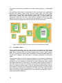
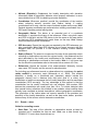
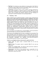
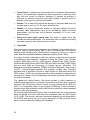
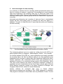
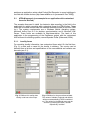
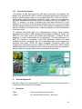
Chapter 4
Individual records and the associated data:
information standards and protocols
by
Alexander Kroupa
European Distributed Institute of Taxonomy (EDIT),
Museum für Naturkunde - Leibniz Institute for Research on Evolution and
Biodiversity
Invalidenstr. 43, 10115 Berlin, Germany
Email: [email protected]
David Remsen
Global Biodiversity Information Facility (GBIF)
Universitetsparken 15, 2100 Copenhagen, Denmark
Email: [email protected]
49
Abstract
The structure of databases with taxonomic content is very important to ensure a
compatibility with other database systems. For the exchange of taxonomic
information it is necessary to have standards and protocols to permit the
presentation, e.g. on a web system like GBIF, of species data from different
database sources. For ATBI+M projects a guideline for recording species has
been developed with the minimal requirements for a high data quality standard.
Also standards are used, errors may occur along the information management
chain from data recording up to data presentation. Error sources can be within
the geo-referenced domain as well as in the taxonomic domain. Therefore
software for automated geo-referencing and recording of date and time in
standardized formats for mobile phones with GPS up to water resistant PDAs
have to be developed. The gain of using those field tools is improving data
quality and simplifying the data recording for a cost effective process to obtain
high quality taxonomic information.
Key words: taxonomic database, standards, data quality, field tools, ATBI+M
50
1.
Introduction
Taxonomic databases – databases that store information about biological
entities: species and other taxa – have been developed to address curatorial
management requirements, taxonomic and scientific needs, and more recently,
for presentation of species data (distribution maps, pictures, biology etc.) to a
wider public (Dalcin, 2005). These databases have the taxon as the principal
entity, represented by its main identification: the taxon name. Taxonomic
databases often have a focus on terminal taxa: species and infraspecies levels,
which consist of a genus and species name, and when applicable, additional
infra-species names. Data or Information is tied to the taxon and typically falls
into two levels of organisation: either elements that relate to the taxon as a whole
or elements that relate to specific instance of a taxon. The latter class of
information is known as species occurrence, or primary occurrence data. Primary
occurrence data include data elements that describe a taxon occurrence such as
a date a species may have been collected or a location where it was observed.
General species data, on the other hand, describe properties ascribe to the entire
taxon such as a general morphological description, or a range map. In this
chapter we will focus on databases for primary occurrence data.
Every day probably more than 100,000 scientific biological records (observations,
collected specimens) are recorded (personal estimation). Many of these data are
still not digitally recorded and the majority of these data are not recorded using
standard protocols or proper referencing. The goal is that all recorded datasets
should be properly referenced and that all individual field records must be
accurately geo-referenced with an exact date or interval. Therefore more and
more electronic tools and software have to be used to facilitate the recording of
species data sets and to minimize the amount of errors.
This chapter provides a review of the important data structure elements of
primary occurrence data with the inclusion of best practices and
recommendations in their use.
2.
Data structure
Species-occurrence data is used to include specimen label data attached to
specimens or lots housed in museums and herbaria (or in Universities, NGOs,
Amateurs associations etc.), observational data (e.g. birdwatchers) and
environmental survey data (Chapman, 2005a). The term has occasionally been
used interchangeably with the term “primary species data”. In general we speak
about “geo-referenced data” – e.g. records with geographic references that tie
them to a particular place in space – whether with a geo-referenced coordinate
(e.g. latitude and longitude, UTM) or not (textual description of a locality, altitude,
depth). Normally, the data are referred to as “point-based”, although line
(transect data from environmental surveys, collections e.g. along a river),
polygon (observations from within a defined area such as a national park) and
grid data (observations or survey records from a regular grid) are also included.
Usually the data are also tied to a taxonomic name, but unidentified collections
51
may also be included by referencing to a higher taxon group (e.g., “Unidentified
Aves”).
For sampling species data it is necessary to record not only where (a geospatial
location) the species were found, but also when (date and time), what
(taxonomy), how (collecting method) and who collected/observed the specimen.
Each locality (where) may have different events (Fig. 1), which means that
sampling at more than one date or with different sampling methods have been
carried out. Each event in turn may have its own species list or even more than
one list if different researchers built their own lists for the same event.
Fig. 1. Context of Locality, Event and Taxonomy by recorded species data.
2.1.
Localities – where
Good locality descriptions lead to more accurate geo-references with smaller
uncertainty values and provide users with much more accurate and high quality
data. When recording data in the field, whether from a map or when using a
GPS, it is important to record locality information as well as the geo-references,
so that later validation can take place if necessary (Chapman & Wieczorek,
2006).
One purpose behind a specific locality description is to allow the validation of
coordinates, in which errors are otherwise difficult to detect. The extent to which
validation can occur depends on how well the locality description and its spatial
counterpart describe the same place. The highest quality locality description is
one with as few sources of uncertainty as possible. By describing a place in
terms of a distance along a path, or by two orthogonal distances from a place,
one removes uncertainty due to imprecise headings. Choosing a reference point
with small extent reduces the uncertainty due to the size of the reference point,
and by choosing a nearby reference point, one reduces the potential for error in
measuring the offset distances.
52
To make it easy to validate a locality, use reference points that are easy to find
on maps or in gazetteers. At all costs, avoid using vague terms such as “near”
and “centre of” or providing only an offset without a distance such as “West of
Albuquerque” (Table 1).
In any locality that contains a named place that can be confused with another
named place of a different type, specify the feature type in parentheses following
the feature name. Data without locality information or only with doubtful details
should be flagged as not possible to geo-reference them with current information.
Vague Localities
BAD: Sacramento River Delta - an extremely large geographic area
BETTER: Locke, Sacramento River Delta, Sacramento Co.,
California - names a town within the Delta
Highway
9,
Alajuela
Province,
Costa
Rica
Names of Roads BAD:
without additional GOOD: Intersection of Hwy 9 and Rio Cariblanco, Cariblanco
points of reference (town), Alajuela Province, Costa Rica
Localities difficult to For many countries, especially Spanish-speaking ones, there are
Georeference
oftentimes several cities with the same name in the same province.
BAD: San Marcos, Intibuca Province, Honduras - There are at least
five
San
Marcos
in
Intibuca
Province
BETTER: San Marcos, ca 7.5 km south of Los Chaguites, Intibuca
Province, Honduras
Table 1. Some examples for good and bad locality descriptions (from Museum of
Vertebrate Zoology 2009a).
Guide for recording localities (Museum of Vertebrate Zoology 2009b)
Full Locality Name. Provide a descriptive locality, even if you have
geographic coordinates. Write the description from specific to general,
including a specific locality, offset(s) from a reference point, and
administrative units such as county, state, and country. The locality should be
as specific, succinct, unambiguous, complete, and accurate as possible,
leaving no room for uncertainty in interpretation. Hint: The most specific
localities are those described by a) a distance and heading along a path from
a nearby and well-defined intersection, or b) two cardinal offset distances
from a single nearby feature of small extent.
53
Altitude (Elevation). Supplement the locality description with elevation
information. Hint: A barometric altimeter, when properly calibrated, is much
more reliable than a GPS for obtaining accurate elevations.
Coordinates. Whenever practical, provide the coordinates of the location
where collecting actually occurred (see Radius, below). If reading
coordinates from a map, use the same coordinate system as the map. Hint:
Decimal degrees coordinates are preferred when reading coordinates from a
GPS and if possible provide lat/long data.
Geographic Datum. The datum is an essential part of a coordinate
description; it provides the frame of the reference. When using both maps
and GPS in the field, set the GPS datum to be the same as the map datum
so that your GPS coordinates will match those on the map. Hint: Always
record the datum with the coordinates.
GPS Accuracy. Record the accuracy as reported by the GPS whenever you
take coordinates. Hint: Most GPS devices do not record accuracy with the
waypoint data, but provide it in the interface showing current satellite
conditions.
Radius (Extent). The extent is a measure of the size of the area within which
collecting or observations occurred for a given locality – the distance from the
point described by the locality and coordinates to the furthest point where
collecting or observations occurred in that locality. Hint: A 1 km linear trap
line for which the coordinates refer to the centre has an extent of 0.5 km.
References. Record the sources of all measurements. Minimally, include
map name, GPS model, and the source for elevation data.
For including geo-referenced records or observations into a database the pointradius method is commonly used (Wieczorek et al., 2004). This method
describes a locality as a coordinate pair (important: always include the
geographic datum!) and a distance from that point (that is, a circle), the
combination of which encompasses the full locality description and its associated
uncertainties (GPS accuracy). The key advantage of this method is that the
uncertainties can be readily combined into one attribute. With modern GPS
devices the uncertainties are usually less than 10 m. To include historical data
from natural history collections this method is also useable, when localities have
typically been recorded as textual descriptions, without geographic coordinates.
The calculation of the radius takes into account aspects of the precision and
specificity of the locality description, as well as the map scale, datum, precision
and accuracy of the sources used to determine coordinates.
2.2.
Events – when
Guide for recording events
54
Start Date. The date of the collection or observation should at least be
recorded and if available the time as well. Hint: use a date format e.g.
DD.MM.YYYY and a time format hh:mm:ss.
End Date. For intervals (e.g. traps which are a longer period in the field) it is
necessary to have a date for the end of the research. Hint: Use the end date
also when the fieldwork takes only a couple of hours.
Collector(s). Provide the name of each collector and when relevant the
name of the expedition or research vessel (i.e. boat). Hint: Do not use
abbreviations, write the full name, including second names or attributes like
senior, junior to identify the collectors uniquely and avoid ambiguity of
homonyms or families of collectors over several generations.
2.3.
Taxonomy – what
Names, whether they are scientific binomials or common names, provide the first
point of entry to most species and species-occurrence databases. The correct
spelling of a scientific name is generally governed by one of the various Codes of
Nomenclature (see list under Technical References). Errors can still occur,
however, through typing errors, ambiguities in the Nomenclatural Code, etc. The
easiest method to ensure such errors are kept to a minimum is to use an
‘Authority File” during recording of data (Chapman, 2004a). An authority file is a
pre-composed list of verified species names. Current lists of species names may
be found at a number of places and some of these are listed in Chapman
(2004b) (e.g. Species2000, FaunaEuropaea, 4D4Life). Also, the re-use of
entered terms via internal controlled lists in an application that provides pull-down
lists of previously entered terms can help maintain consistency when a controlled
list is not available.
If it is not possible to use authority lists, a recommendation is than to process the
collected information as quickly as possible after the fieldwork.
The structure of the database has to be clear, unambiguous and consistent. The
taxon information should be atomized so that it is always clear that one field
includes just the genus or the species name and is not mixed to have just one
field with the genus and the species name together. One should always atomize
the taxonomic information into separate Genus/Species/infraspecific
Rank/Infraspecies/Author fields etc. wherever possible.
Guide for recording the minimum taxonomy for species-level taxa
Genus name. The genus name is essential. Hint: Do not use any
abbreviation.
Species name. The species name is essential. Hint: Do not use any
abbreviation.
Authors of a species name. The author(s) name should be included to
ensure a unique mapping in case of homonyms.
Determinator. The name of the person(s) who is responsible for the
determination of the collection/observation. Hint: Do not use any
abbreviation, write the full name.
55
Taxon Source. A reference to a taxonomic guide or treatment that forms the
basis for the identification. Species are often lumped with or split from other
taxa over the course of revisions. Ambiguity is reduced by providing a
reference to particular taxonomic view that provides a specific sense or
definition of the taxon as used by the identifier.
Number. The number of the individuals observed or collected. Hint: Use only
numbers and no text (not 2-3, 3ff, some, abundant etc.)
Deposit. For further studies the deposit of collected material should be
recorded. Hint: Abbreviations have to be well-defined, better do without
abbreviations. Add the town of the museum, especially if it is not a wellknown museum.
Family and other higher parent taxa. The family or higher taxon that
includes the referenced species. This information may be useful for providing
taxonomic context in later references to the record.
3.
Standards
Since more and more taxonomic databases are appearing, both institutional and
individual concern about sharing data is rising. At this moment the need to
establish data standards and communication protocols is obvious in order to
make data sharing between different databases possible (Dalcin, 2005).
A number of recent collaborations within the museum community have resulted
in establishing data standards. Examples include the Darwin Core Schema
(Vieglais, 2003) along with the DiGIR protocol (SourceForge, 2004) and the
combined BioCASE protocol (BioCASE 2003) and ABCD schema (TDWG, 2004)
that are more fitted for interchange of primary species information. The
Biodiversity Information Standards (TDWG) and others developed a new protocol
(TAPIR - http://ww3.bgbm.org/tapir) that supports multiple data formatting
standards that is intended to provide a single solution for publishing data to the
GBIF network. TAPIR can be implemented in multiple degrees of complexity and
capacity (lite, medium, full) but importantly, still require advanced technical skills
to install and maintain.
The newest and ratified Darwin Core terms provides a unified approach to
publishing both species-level and species-occurrence-level data using a common
standard. This "DarwinCore Archive" format is being championed by GBIF and
while it is a supported output of the Integrated Publishing Toolkit, provides a
simple enough data publication solution that it can be output as a direct database
export by many data managers.
For recording geo-referenced species data a guideline with the most important
fields for species occurrence data has been developed within the EDIT project
(EDIT, 2009). This structure has been developed especially for recording data in
the ATBI+M sites and is used by everyone sampling for ATBI purposes. It may
also be used as a base for creating own databases.
56
4.
Errors
4.1.
Sources of error in data (Hellerstein, 2008)
Data entry errors. It remains common in many settings for data entry to be
done by humans, by keying in data from written or printed sources, e.g. after
fieldwork. In these settings, data is often corrupted at entry time by
typographic errors or misunderstanding of the data source (see 2.3).
Measurement errors. In the measurement of physical properties, as altitude
or spatial data, the increasing proliferation of sensor technology has led to
exact measurements. Nevertheless data errors are still quite common:
selection and placement of sensors often affects data quality, and by
transferring data to the database errors may occur. Converting coordinates
from one system to another may cause errors and converting
longitude/latitude data from degrees to decimal may often result in a wrong
calculation (Table 2).
Distillation errors. In many settings, raw data are preprocessed and
summarized before they are entered into a database. This data distillation is
done for a variety of reasons and has the potential to produce errors in
distilled data, or in the way that the distillation technique interacts with the
final analysis.
Data integration errors. Any procedure that integrates data from multiple
sources can lead to errors. To minimize integration errors standards are
necessary to ensure that fields contain the same entity type. That e.g. a
species field contains only the species epithet and not genus and epithet
together.
latitude / longitude
formula
calculation
decimal result
44° 16’ 12,01’’ - 7° 23’ degrees + (minutes / 44 + (16 / 60) + (12,01 / 44,27000278°
7,39680556°
3600) / 7
60) + (seconds /
48,50’’
3600)
+ (23 / 60) + (48,50 /
3600)
44° 15,368’ - 7° 22,86’
degrees + (minutes / 44 + (15,368 / 60) / 7 + 44,2728° - 7,381°
60)
(22,86 / 60)
Table 2. Two examples to show how to convert longitude/latitude data from degrees to
decimal.
Names form the major key for accessing information in primary species
databases. If the name is wrong, then access to the information by users will be
difficult, if not impossible. Table 3 shows what may happen when entering names
in a non-standard way. This is an extreme example but misspellings of names
are the most frequent error in taxonomic databases.
57
Actinobacillus
actimomycetemcomitans
Actinobacillus
actinomycetecomitans
Actinobacillus
actinomycetum
Actinobacillus
actimycetemcomitans
Actinobacillus
actinomycetemcmitans
Actinobacillus
actinomyctemcomitans
Actinobacillus
actinmycetemcomitans
Actinobacillus
actinomycetemcomintans
Actinobacillus
actinomyectomcomitans
Actinobacillus
actinomicetemcomitans
Actinobacillus
actinomycetemcomitance
Actinobacillus
actinomyetemcomitans
Actinobacillus actinomy
Actinobacillus
actinomycetemcomitans
Actinobacillus
actinonmycetemcomitans
Actinobacillus
actinomycetemcomitants
Actinobacillus
actionomycetemcomitans
Actinobacillus
actinomycetemcommitans
Actinobacillus
actynomicetemcomitans
Actinobacillus
actinomycetemocimitans
Actinobacillus
antinomycetemcomitans
Actinobacillus actinomyce
Actinobacillus
actinomycemcomitans
Actinobacillus
actinomyceremcomitans
Actinobacillus
actinomycetam
Actinobacillus
actinomycetamcomitans
Actinobacillus
actinomycetencomitans
Table 3. Result of non-standard data entry for the valid species Actinobacillus
actimomycetemcomitans (source: from Neil Sarkar, uBio Project).
4.1.
Data cleaning
Chapman (2005a) shows that the cost of error correction increases as one
progresses along the Information Management Chain (Fig. 2) and a manual
process of data cleansing is also laborious, time consuming, and itself prone to
errors (Maletic & Marcus, 2000). Tools have to be developed for data cleaning
and preventing of errors at their point of origin is the most cost-effective method.
Tools are being developed to assist the process of adding geo-referencing
information to databased collections. Such tools include eGaz (Shattuck, 1997),
geoLoc (CRIA, 2004), BioGeomancer (Peabody Museum n.dat.), GEOLocate
(Rios and Bart n.dat.) and the Georeferencing Calculator (Wieczorek, 2001).
The most important point is that correcting problems and adding sufficient
annotation for use should be done prior to, not after, publication of the data. Data
validation and annotation services should be done by the curator, not after the
data has been published and copies transferred. When services are run against
a copy of the data they need to be transferred and reconciled with the source
copy, increasing complexity and risking the introduction of new errors. This
approach will not apply to the many legacy datasets that are no longer curated so
there will always be a need for the application of validation and annotation
services as post-publication processes as well.
58
5.
New technologies for data recording
It is necessary to develop tools for recording spatial and taxonomic data in the
field for a number of reasons. In particular it is cost-effective to avoid mistakes
right at the beginning of the recording chain (Fig. 2). Each error which is not
made saves a lot of time. Errors may be avoided by using authority lists, e.g. for
countries, habitat-types or species groups that can be determined to a great part
in the field.
Automated geo-referencing and recording of date and time in standardized
formats will also avoid typing errors by rewriting the data from paper to a
database. The gain of using field tools is improving data quality and simplifying
the data recording.
Fig. 2. Information Management Chain showing that the cost of error correction increases
as one progresses along the chain (modified from Chapman, 2005a).
The developed software has to be usable for mobile phones with GPS up to
water resistant PDAs (e.g. Magellan - Mobile Mapper; Trimble – Juno, Nomad).
For ArcPad (software from ESRI Inc.) some applications are already developed
for recording data in the field for different types of use. One application is for
birdwatchers and it focuses on birding sites near Gainesville (Wakchaure, 2006).
Another application with customized ArcPad forms was developed for an
earthworm inventory to be conducted during summer 2004 (Dabrowski, 2004).
This study would measure the impact of European earthworm invasions on
vegetation and soil characteristics at two Great Lakes national parks (Pictured
Rocks National Lakeshore, located in the Upper Peninsula of Michigan, and
Voyageurs National Park, located in northern Minnesota).
Another software for ecological data entry is Pocket eRelevé
(http://ereleve.codeplex.com/ [accessed 4 Dec. 2009]) designed for naturalists.
This program is developed in Visual Basic and only available in French. For bird
59
watchers an application exists called Pocket Bird Recorder to record sightings in
the field with mobile devices (http://www.wildlife.co.uk [accessed 4 Dec. 2009]).
5.1.
ATBI+M approach (one example for an application with customized
forms for ArcPad)
The example discussed in detail for electronic data recording in the field is the
application for mobile recording with customized forms for ATBI+M sites. These
forms are for mobile devices with the installed software ArcPad (a tool from ESRI
Inc.). The system requirements are a Windows Mobile operating system,
Microsoft Active Sync 4.5 for desktop synchronization and a Microsoft XML
Parser. These forms are available at http://www.atbi.eu. The basis of this
application is the programming of the Earthworm project with the customized
ArcPad forms for selecting species, named Species Picker (Dabrowski, 2004).
5.1.1.
Locality forms
For recording locality information, two customized forms exist. On the first form,
(Fig. 3) a code and a name for the locality is arbitrary. The country can be
selected from a list box and specifications to the macrohabitat and remarks can
be made (see 2.1).
Fig. 3. Editform for Locality data.
Locality code has to be unique.
60
Fig. 4. Editform for the geo-referenced data.
The values of latitude, longitude and altitude
will be set automatically (if GPS is switched
on). The values for the altitude range can be
set also by pressing the button “set Min”
respectively “set Max”.
On the second form, (Fig. 4) information to the geo-referencing of the locality can
be filled in. Latitude, longitude, accuracy and the minimum altitude are filled in
automatically. The minimum and maximum altitude may be set with the two
buttons “set Min” and “set Max” in the case the research area is not on one
altitude level. But it is also possible to write values into these fields if other tools
for measuring the altitude are used. Everybody has to bear in mind that the
accuracy of the altitude measurement with GPS tools is very low. It is about 10
times lower than the accuracy for longitude or latitude.
The used coordinate system can be selected with a list box.
5.1.2.
Event forms
For each locality more than one event can be created (see 2.2). Therefore a form
exists to list all existing events for one locality (Fig. 5). The events are listed
chronological with the start date of the events. Each event can be edited or
deleted (deleting will delete also the attached species list).
Fig. 5. List of all events belonging to one
Locality ordered in chronological sequence.
Fig. 6. Editform for one event. The value
of the start time will be set automatically.
The values for the start time and end
time can be set also by pressing the
button “set Start” respectively “set End”.
61
The detail data for each event consists of one EventCode and of the start and
the end date (time) of this event (Fig. 6). The start date will be created
automatically by creating a new event. The format for the date is [DD.MM.YYYY
hh:mm:ss]. With the buttons “set Start” and “set End” the current time will be filled
into the adequate fields. The collector, the collecting method and remarks can
also be added to each event.
5.1.3.
Species forms
For each event a species list of observed or collected specimens can be created.
Therefore a species has to be selected on the page “All Species” (Fig. 7) from an
authority species list (dbf-file). This file can be created by researchers
themselves and can be exchanged easily for using different species groups (see
2.3 and 4.1). With the button “Add” the selected species will be transferred to the
species list of this event. For each species the sex and the number of
observed/collected specimens can be selected.
On the page “Event Species” (Fig. 8) all selected species are listed with
information to the sex and the number of individuals. The records can be
removed by selecting one entrance and pressing the button “Remove Selected”.
Wrong entries of numbers can be corrected by choosing on the Page “All
Species” the species which has to be corrected with the correct number of
individuals. After pressing the “Add” button the correction has to be confirmed
and then the new number of individuals is saved.
Fig. 7. List of all species that can be
selected. For each species the sex and the
number of individuals can be added.
62
Fig. 8. List of species for one event. For
each species the number of recorded
specimens and their sex are available in
brackets. (f female; m male; ? unknown).
5.2.
From field to the web
The transfer of data from the field to the web environment via networks and
portals such as BioCASE, GBIF or WDPA (http://www.wdpa.org) is necessary in
order to provide global access to the sampled data (Fig. 9). All the records –
observations, collected specimens or literature data – have to be transferred to
an online database that provides access, for example through a “wrapper” for
GBIF. A “wrapper” is a piece of software that maps data contained in a local
database to a common data exchange standard and then serves these data
through standard exchange protocols. This allows different databases to publish
data to a network in a common form – enabling integration and the development
of common tools.
To integrate biodiversity data from heterogeneous sources using common
standards and protocols, GBIF developed the Integrated Publishing Toolkit. The
GBIF IPT is an Open source Java based web application. It embeds its own
database, is easily customisable and is multilingual. The data registered in a
GBIF IPT instance is connected to the GBIF distributed network and made
available for public consultation and use via established data access formats and
protocols that include TAPIR and Open Geospatial Consortium (OGC) web
mapping and web feature services (WMS and WFS) (Réveillon, 2009). Simple
transformations of the DarwinCore Archive file would also support the creation of
Keyhole Markup Language (KML) files for use within Google earth.
Fig. 9. Data flow from the field recording with GPS tools to different internet presentations.
6.
Acknowledgements
We wish to thank A.D. Chapman and J. Wieczorek who, due to their publications,
created a profound basis for this chapter.
7.
Acronyms
ABCD
Access to Biological Collections Data
ATBI+M
All Taxa Biodiversity Inventory + Monitoring
63
BioCASE
Biological Collection Access Service
DiGIR
Distributed Generic Information Retrieval
GBIF
Global Biodiversity Information Facility
GPS
Global Positioning System
IPT
Integrated Publishing Toolkit
KML
Keyhole Markup Language
OGC
Open Geospatial Consortium
TAPIR
TDWG Access Protocol for Information Retrieval
TDWG
Taxonomic Databases Working Group
UTM
Universal Transverse Mercator
WDPA
World database on protected areas
WFS
web feature services
WMS
web mapping features
8.
Key links
Access to Biological Collection Data (ABCD)
http://wiki.tdwg.org/twiki/bin/view/ABCD/ [accessed 4 Oct. 2009] (TDWG Wiki for ABCD)
http://www.bgbm.org/tdwg/codata/schema/ABCD_2.06/HTML/ABCD_2.06.html
Schema) [accessed 4 Oct. 2009]
(XSLT
DIVA-GIS
http://www.diva-gis.org [accessed 4 Oct. 2009]
Environmental Resources Information Network (ERIN)
http://www.deh.gov.au/erin/index.html [accessed 4 Oct. 2009]
GEOLocate – University of Tulane
http://www.museum.tulane.edu/geolocate/ [accessed 4 Oct. 2009]
Mammal Networked Information System (MaNIS)
http://manisnet.org/ [accessed 4 Oct. 2009]
http://manisnet.org/Documents.html (MaNIS Documents) [accessed 4 Oct. 2009]
http://manisnet.org/GeorefGuide.html (Georereferencing Guidelines) [accessed 4 Oct.
2009]
Museum of Vertebrate Zoology Informatics (MVZ) – University of California,
Berkeley
http://mvz.berkeley.edu/Informatics.html [accessed 4 Oct. 2009]
64
http://mvz.berkeley.edu/Locality_Field_Recording_Notebooks.html (Guide for Recording
Localities in the Field) [accessed 4 Oct. 2009]
http://mvz.berkeley.edu/Locality_Field_Recording_examples.html (Examples of Good and
Bad Localities) [accessed 4 Oct. 2009]
http://mvz.berkeley.edu/Locality_Field_Recording_important.html (Why it is Important to
Take Good Locality Data) [accessed 4 Oct. 2009]
OGC Recommendations Document Pointer
http://www.opengeospatial.org/standards/is [accessed 4 Oct. 2009]
9.
References
BIOCASE 2003. Biological Collection Access Service for Europe. [see
http://www.biocase.org - accessed 4 Oct. 2009].
CHAPMAN, A.D. 2004a. Environmental Data Quality – b. Data Cleaning Tools.
Appendix I to Sistema de Informação Distribuído para Coleções Biológicas: A
Integração do Species Analyst e SinBiota. FAPESP/Biota process no.
2001/02175-5 March 2003 – March 2004. CRIA, Campinas, Brazil. 57 pp. [see
http://splink.cria.org.br/docs/appendix_i.pdf - accessed 30 Sep. 2009].
CHAPMAN, A.D. 2004b. Guidelines on Biological Nomenclature. Brazil edition.
Appendix J to Sistema de Informação Distribuído para Coleções Biológicas: A
Integração do Species Analyst e SinBiota. FAPESP/Biota process no.
2001/02175-5 March 2003 – March 2004. CRIA, Campinas, Brazil. 11 pp. [see
http://splink.cria.org.br/docs/appendix_j.pdf - accessed 30 Sep. 2009].
CHAPMAN, A.D. 2005a. Principles of Data Quality, version 1.0. Report for the
Global Biodiversity Information Facility, Copenhagen.
CHAPMAN, A.D. 2005b. Uses of Primary Species-Occurrence Data, version 1.0.
Report for the Global Biodiversity Information Facility, Copenhagen.
CHAPMAN, A.D. & WIECZOREK, J. (Eds) 2006. Guide to Best Practices for
Georeferencing. Global Biodiversity Information Facility, Copenhagen. [see
www.gbif.es/ficheros/Colombia/Georeferencing_Best_Practices.pdf - accessed
24 Jun. 2009].
CRIA 2004. GeoLoc-CRIA. Campinas: Centro de Referência em Informação
Ambiental. [see http://splink.cria.org.br/tools/ - accessed 4 Oct. 2009].
DABROWSKI, J. 2004. Experiences developing a custom ArcPad solution for an
Earthworm Inventory.
[see http://science.nature.nps.gov/im/units/mwr/documents/APExperiences.pdf accessed 4. Oct. 2009].
DALCIN, E.C. 2005. Data Quality Concepts and Techniques Applied to Taxonomic
Databases. University of Southampton – Faculty of Medicine, Health and Life
Sciences, 266 pp.
EDIT 2009. Data recording guidelines for ATBI+M pilot sites. [see
http://www.atbi.eu/wp7/files/common/Excel_sheet_for_locality_and_event_entry.
xls - accessed 30 Sep. 2009].
65
HELLERSTEIN, J.M. 2008. Quantitative data cleaning for large databases. White
paper, United Nations Economic Commission for Europe. 42 pp. [see
http://db.cs.berkeley.edu/jmh/papers/cleaning-unece.pdf - accessed 21 Sep.
2009].
MALETIC, J.I. & MARCUS, A. 2000. Data Cleansing: Beyond Integrity Analysis.
Division of Computer Science, Department of Mathematical Sciences, The
University of Memphis, Memphis, 10 pp.
MUSEUM OF VERTEBRATE ZOOLOGY 2009a. Examples of Good and Bad Localities.
[see
http://mvz.berkeley.edu/Locality_Field_Recording_examples.html
accessed 18 Sep. 2009]
MUSEUM OF VERTEBRATE ZOOLOGY 2009b. MVZ Guide for Recording Localities in
Field Notes. [see http://mvz.berkeley.edu/FieldLocalities.doc - accessed 18 Sep.
2009]
PEABODY MUSEUM n.dat. BioGeoMancer. [see http://www.biogeomancer.org accessed 4 Oct. 2009].
RÉVEILLON, A. 2009. The GBIF Integrated Publishing Toolkit User Manual,
version 1.0. Global Biodiversity Information Facility, Copenhagen. 37 pp. [see
http://gbif-providertoolkit.googlecode.com/files/GBIF_IPT_User_Manual_1.0.pdf accessed 3 Dec. 2009].
RIOS, N.E. & BART, H.L.JR. n.dat. GEOLocate. Georeferencing Software. User’s
Manual. Belle Chasse, LA, USA: Tulane Museum of Natural History. [see
http://www.museum.tulane.edu/geolocate/support/manual_ver2_0.pdf
accessed 4 Oct. 2009].
SHATTUCK, S.O. 1997. eGaz, The Electronic Gazetteer. ANIC News 11: 9.
SOURCEFORGE 2004. Distributed Generic Information Retrieval (DiGIR). [see
http://digir.sourceforge.net/ - accessed 4 Oct. 2009].
TDWG 2004. ABCD Schema – Task Group on Access to Biological Collection
Data.
[see
http://bgbm3.bgbm.fu-berlin.de/TDWG/CODATA/default.htm
accessed 4 Oct. 2009].
VIEGLAIS, D. 2003. The Darwin Core. Revision 1.5. Lawrence, KA: University of
Kansas Natural History Museum and Biodiversity Research Center.
WIECZOREK, J. 2001. MaNIS/HerpNet/ORNIS Georeferencing Guidelines. [see
http://manisnet.org/GeorefGuide.html - accessed 30 Sept. 2009].
WIECZOREK, J., GUO, Q. & HIJMANS, R.J. 2004. The point-radius method for
georeferencing locality descriptions and calculating associated uncertainty. Int. J.
Geographical Information Science 18(8): 745-767.
WAKCHAURE, A. 2006. An Application for Birdwatchers – Final Report. [see
http://ashwinimail.web.officelive.com/Documents/0_website_GPS_birding_app.p
df - accessed 4 Oct. 2009].
66
10. Technical References
FRANCKI, R.I.B., FAUQUET, C.M., KNUDSON, D.L. & BROWN, F. 1990. Classification
and Nomenclature of Viruses. Archives of Virology, Suppl. 2: 1-445.
INTERNATIONAL CODE OF BOTANICAL NOMENCLATURE 2000. International Code of
Botanical Nomenclature (St Louis Code). Regnum Vegetabile 138. Königstein:
Koeltz
Scientific
Books
[see
http://www.bgbm.fuberlin.de/iapt/nomenclature/code/SaintLouis/0001ICSLContents.htm - accessed
4 Oct. 2009].
INTERNATIONAL CODE OF ZOOLOGICAL NOMENCLATURE 2000. International code of
zoological nomenclature adopted by the International Union of Biological
Resources International Commission on Zoological Nomenclature. 4th edition.
London:
International
Trust
for
Zoological
Nomenclature.
[see
http://www.iczn.org/iczn/index.jsp - accessed 4 Oct. 2009].
SNEATH, P.H.A. (Ed.) 1992. International Code of Nomenclature of Bacteria, 1980
Revision. Washington: International Committee on Systematic Bacteriology
(ICSB). [see http://www.ncbi.nlm.nih.gov/bookshelf/br.fcgi?book=icnb - accessed
4 Oct. 2009].
TREHANE, P., BRICKELL, C.D., BAUM, B.R., HETTERSCHEID, W.L.A., LESLIE, A.C.,
MCNEILL, J., SPONGBERG, S.A. & VRUGTMAN, F. 1995. International Code of
Nomenclature for Cultivated Plants. Winbourne, UK: Quarterjack Publishing. [see
http://www.ishs.org/sci/icracpco.htm - accessed 4 Oct. 2009].
67