Download FORCinel Guide.pages

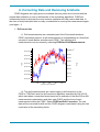
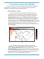
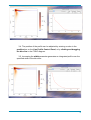
FORCinel processing
2015 First Order Reversal Curve (FORC) Workshop – July 23-24, 2015
1
FORCinel processing
1
1. Introduction
3
2. Installation
4
3. The Basic Igor Environment
5
4. Loading a FORC file
6
5. Optional pre-processing steps
8
6. Initial FORCinel processing
9
7. Visualisation Options
11
8. Correcting Data and Removing Artefacts
14
9. Quantitative analysis
22
10. VARIFORC processing
27
11. Choosing the VARIFORC parameters
30
12. Quantitative analysis with VARIFORC
34
13. Troubleshooting
41
14. References
43
2
1. Introduction
First-order reversal curve (FORC) analysis is an advanced hysteresis measurement
that is becoming a standard tool in magnetic studies. FORC diagrams offer the possibility
of unambiguous domain-state fingerprinting, calculation of a range of coercivity
distributions, quantification of inter- and intra-particle interactions, quantitative analysis of
multi-phase mixtures and identification of magnetic impurities. FORC diagrams are
increasingly being used as a basis of comparison with modelling studies, allowing the
underlying physics of the system to be explored.
Obtaining and analysing a FORC diagram requires the use of data processing
software. There are several packages available, most of which require the use of auxiliary
software to run:
Name
Author
URL
Requires
FORCinel
Richard Harrison
https://
wserv4.esc.cam.ac.uk/
nanopaleomag/
Igor Pro
VARIFORC
Ramon Egli
http://www.conradobservatory.at/
cmsjoomla/en/
download/category/5variforc
Mathematica
FORCit
Gary Acton
http://
paleomag.ucdavis.edu/
software-forcit.html
None
butterFORC
Xiang Zhao
https://
sites.google.com/site/
butterforc/home
Labview
Each of these packages has their pros and cons. There is reasonable feature parity
between FORCinel and VARIFORC, although the interface philosophies are quite
different.
This user guide describes practical aspects of processing using FORCinel. For a
guide to the theory of FORC diagrams I recommend visiting Ramon Egli’s VARIFORC site
and downloading his excellent documentation, which contains useful FORC tutorials,
background theory and processing guides that are (mostly) also applicable to FORCinel.
3
2. Installation
Visit the FORCinel download page:
https://wserv4.esc.cam.ac.uk/nanopaleomag/?page_id=51
If you do not have Igor Pro installed on your machine then follow the link to the Igor
Pro demo download page on the Wavemetrics site and follow the instructions there to
install Igor Pro. You get a free 30 days license. After this, you will still be able to run
FORCinel, but will no longer be able to save or export data. A full license costs $435 for
non-students and only $85 for students. Igor is also required to run FORCulator and
FORCem, so well worth the investment!
Next download the FORCinel package. This is a zip archive containing the
FORCinel package (an Igor Pro packed experiment file, extension .pxp), two test data files
and a READ ME text file containing information on the current and past versions:
Double click the FORCinel v2.04.pxp file to open Igor Pro and run FORCinel.
4
3. The Basic Igor Environment
FORCinel menus
FORCinel control panel
Data Browser
History
Command Line
FORCinel is operated primarily through the FORCinel and FORCinextras menus.
Some of the most common functions are also included in the FORC Control Panel for
easy access.
The FORCintense menu is an implementation of Adrian Muxworthy’s FORC
paleointensity method. We anticipate that this method will be superseded by the KMC
option within FORCulator in the near future, so will not discuss it here.
Other menus are not specific to FORCinel, but will be of use in certain
circumstances. The Data menu gives you access to the Data Browser window, which
contains a list of all the FORC data you have loaded in and allows you to switch between
different datasets; the Graph menu, controls aspects of how FORC diagrams are plotted;
the Image menu contains image processing functions, including the ability to generate
horizontal and vertical profiles when working with VARIFORC data.
The Command Line is normally the main way a user interacts with Igor. FORCinel,
however, is designed to be used entirely from the menus and you will rarely have to type
commands. The History area keeps a log of various actions that have been performed
and also reports certain quantitative measurements extracted from the FORC data.
5
4. Loading a FORC file
1. To load a FORC file either go to FORCinel: Load FORCs or click the Load
FORC file button on the FORC Control Panel.
2. Navigate the file system to the desired data file and click Open. In this case we
will choose the bush.txt test file delivered in the FORCinel download folder.
3. The raw data will load and you will be presented with a plot of the raw FORC
curves.
4. Note that a new folder named bush.txt appears in the Data Browser window,
and that the red arrow now points at this folder, signifying that this is the active data
folder. All FORCinel menu actions are applied to the active folder. To change the
active folder, drag the red arrow to point at another folder. 5. Click on the blue expansion arrow just to the right of the red arrow to expand the
folder and see its contents. You will see a number of data objects (in the Igor universe
we refer to these as ‘waves’). These include the drift field and drift magnetisation
measurements, the individual FORC field and magnetisation measurements (wave0,
wave1, wave2, etc), as well as various parameters loaded in from the header of the
data file. Other waves will appear after you process the FORC data. You will not
6
normally need to interact with these waves directly, so click the blue arrow again to
collapse the folder.
6. By default, all of the measured FORC curves are plotted when data is first
loaded. It can often be difficult to distinguish individual curves. To plot only a subset of
the measured FORCs select FORCinel: Display FORCs. When prompted, enter a
number, n, to display only every nth FORC curve. This option can be used at any time
to plot raw FORC curves (remember: always make sure the red arrow is pointing at the
folder containing the data you want to plot).
7. You probably now have two FORC plots. Close one or both of them by clicking
the window close button. Whenever you close a window you will be asked whether you
want to save a window recreation macro. This saves the list of instructions required
to regenerate the window. Saved windows will appear in Windows: Graph Macros for
later retrieval. Unless you have heavily customised a plot, there is usually no need to
save a window recreation macro: most plots can be regenerated via the FORCinel
menus.
(TIP: If you want to prevent the window save macro dialogue coming up every time you
close a window, press the ALT key when you click the window close button).
7
5. Optional pre-processing steps
Before you process the FORC data and plot the FORC diagram, there are a few
optional pre-processing steps you might want to take advantage of:
1. If your original data were recorded using cgs units (Oersteds and emu), the
option FORCinextras:Convert cgs to SI units will convert the data to SI units (Tesla
and Am2). Rather than overwrite the original data, a new data folder with prefix “SI_” is
generated containing the converted data. The new data folder is automatically selected
as the active folder for further processing.
2. The option FORCinextras:Mass Normalise FORC Data will convert to a mass
normalised magnetisation (e.g. Am2/kg in SI units). The software will prompt you to
enter the mass of the sample in grams and then generate a new data folder with prefix
“MassNorm_” containing the normalised data. The new data folder is automatically
selected as the active folder for further processing.
3. The above options can be used sequentially to convert from cgs to SI units and
then to mass normalised SI units.
4. To save memory and disc space, after conversion you may want to choose to
delete the original data folder. To do this select the folder by clicking on it, and then
press the Delete button on the Data Browser. (Note: you cannot delete a folder if
any of the data within it form part of an existing plot. Close any plots involving
data from the target folder before pressing the Delete button).
8
6. Initial FORCinel processing
You are now ready to process the data and produce an initial FORC diagram. In
FORCinel, the first step is to always to process the data using the LOESS smoothing
method described by Harrison and Feinberg (2008). 1. Select FORCinel:Process FORCs or press the Process FORC button on the
FORC Control Panel. The Process FORCs function performs two operations: i) it
converts the individual raw FORC curves into the matrix form required by the LOESS
smoothing operation, and ii) it performs the LOESS smoothing with a specified
smoothing factor to generate the FORC diagram. Please note the following:
1.1.You only need to perform FORCinel:Process FORCs once per data set.
After that, use FORCinel:Change Smoothing Factor or press the Change
Smoothing button on the FORC Control Panel to control the level of smoothing.
1.2. Initial processing is performed on the raw data without drift correction.
Drift correction can be performed after the initial processing if required (see
Section 8).
2. The software prompts you to enter a smoothing factor. Since there is no way to
know in advance what value is the best, begin with a value of 1 and then go from
there.
9
3. After a few seconds to minutes (depending on the size of the dataset) the
processed FORC diagram will appear. If the window appears blank, or there an error,
or no recognisable FORC signal is present, please take a look at Section 13:
Troubleshooting before emailing the author! You can display the processed FORC
diagram any time by selecting FORCinel:Display Processed FORCs (cmd+d on Mac,
ctrl+d on Windows).
4. Explore the effect of changing smoothing factor by pressing the Change
Smoothing button on the FORC Control Panel. Note that the reduction in noise with
higher smoothing factors comes at the expense of an increasingly smeared out and
distorted signal. Choosing the right smoothing factor is a compromise between these
two competing effects.
5. A guide to the optimum compromise can be obtained using the
FORCinel:Calculate Optimum Smoothing Factor function. Smoothing factors are
automatically increased from a minimum to a maximum value, with a specified step
size. At each step the standard deviation of the residual between the measured
magnetisation data and the smoothed magnetisation surface is analysed. The residual
increases initially as noise is removed, forms a plateaux near the optimum smoothing
factor, then increases again as excessive smoothing begins to distort the processed
FORC diagram. The optimum smoothing factor is estimated as the inflection point of
the residual vs smoothing factor curve. You may want to run the algorithm a few times
in order to optimise the smoothing factor range and step size appropriately. For the
bush.txt file the optimum smoothing factor is close to 3. Once determined, the FORC
diagram is automatically processed using the optimum smoothing factor. Optimum SF = 3
10
7. Visualisation Options
After initial processing, there are many options to optimise the way the FORC
diagram is displayed.
1. Optimise the colour intensity range:
1.1. The default intensity range of the colour scale is automatically selected
according to the minimum and maximum FORC signals in the whole FORC
diagram. This default intensity scale can be reached at any time by either selecting
FORCinel:Reset to Default Intensity Range (shortcut cmd+2 on Mac, ctrl+2 on
Windows) or by pressing the Reset Colour Scale button on the FORC Control
Panel.
1.2. You can optimise the intensity range according to the minimum and
maximum FORC signals contained within a subsection of the FORC diagram (e.g.
avoiding any strong artefact signals). Click and drag across the region of interest to
create a marquee selection:
Before
After
Then select FORCinel:Autoscale Intensity Range (cmd+1 on Mac, ctrl+1 on
Windows). You can explore different region selections, and can always get back to
the default values using the Reset Colour Scale button on the FORC Control
Panel.
11
2. Choose the colour scale
2.1. FORCinel comes with some default preset colour scales. You can switch
between these using the Select Preset variable on the FORC Control Panel. If
you prefer the old school rainbow colour scheme (not recommended) then you can
switch between the Rainbow Colour Scheme and the Default Colour Scheme
using the buttons on the FORC Control Panel.
2.2. For the default colour scheme, the number of discrete colours used to define
the colour scale can be controlled using the Number of Colours popup on the
FORC Control Panel. By restricting the number of colours used, a useful colour
contouring effect can be achieved. This feature can also be useful for hiding
unwanted background noise without adversely affecting the display of the real
signal.
2.3. Colour scales can be fine tuned by pressing the Fine Tine Colourscale
button on the FORC Control Panel:
The sliders control the intensity, position and width of tanh-like changes in the Red,
Green and Blue channels of the RGB colour scale. Separate sliders for intensity
and width of the blue scale used for negative signals are also provided. With some
random fiddling, adjustments can be made to suit different data. If you like a
particular colour combination you can save it as a preset by pressing the Save
Preset button. This will now be selectable from the Select Preset variable on the
FORC Control Panel.
12
(TIP: The colour scale presets are stored in a 2D wave called preset0 located in
the ColourScales Data Folder. To edit this wave, double click it in the Data
Browser. Each column of 11 values corresponds to a given preset. You can copy
these values into different FORCinel experiments to transfer your own presets, or
manually delete presets you don’t like by highlighting the appropriate column and
selecting Edit:Cut).
3. Add contours
3.1. To add contours to the FORC diagram select FORCinel: Add Contours.
The intensity range covered by the contours is automatically selected according to
the minimum and maximum FORC signals in the whole FORC diagram. This
default contour range can be reached at any time by selecting FORCinel:Reset to
Default Contour Range (shortcut cmd+4 on Mac, ctrl+4 on Windows).
3.2. You can optimise the contour range according to the minimum and maximum
FORC signals contained within a subsection of the FORC diagram (e.g. avoiding
any strong artefact signals). Click and drag across the region of interest to create a
marquee selection. Then select FORCinel:Autoscale Contour Range (cmd+3 on
Mac, ctrl+3 on Windows). You can explore different region selections, and can
always get back to the default values using FORCinel:Reset to Default Contour
Range.
3.3. Most aspects of the contour display can be controlled via Graph:Modify
Contour Appearance…. This allows you to change the number, colour, line style,
and labelling of contours. The appearance of individual contour lines can be
controlled by double clicking on the contour line in the FORC plot.
3.4. To remove contours from the FORC diagram, go to Graph:Remove from
Graph…, select Contours from the pop-up list, select M_RotatedImage from the
wave list, and then click Do It.
4. Other display options
4.1. You can plot the FORC diagram in the original unrotated coordinate system
by choosing FORCinextras:Display Unrotated FORC Diagram.
4.2. You can plot the raw FORCs coloured according to the FORC distribution by
selecting FORCinextras:Display Coloured FORC curves. (TIP: This works best
with VARIFORC processed data).
13
8. Correcting Data and Removing Artefacts
FORC diagrams are highly prone to artefacts that may arise due to issues with the
original data collection or due to deficiencies of the smoothing algorithms. FORCinel
incorporates tools to eliminate the most common artefacts and help rescue bad data. In
the case of really bad data there is really no substitute for running the measurement again
(and again…)!
1. Drift correction
1.1. Drift measurements are a standard part of the Princeton/Lakeshore
FORC acquisition protocol. A drift measurement of magnetisation at a fixed field
set point is made before and after each FORC. The resulting drift
measurements can be viewed by selecting FORCinel:Drift Measurements:
-3
9.428x10
4612.98
9.426
4612.96
9.424
9.422
Drift Field
Drift Mag
4612.92
9.420
4612.90
Mag
Field
4612.94
9.418
4612.88
9.416
4612.86
9.414
4612.84
0
20
40
60
80
Measurement Number
100
1.2. The drift measurements are used to apply a drift correction to the
FORCs. FORCinel uses the drift correction algorithm described by Egli (2013),
which calculates a correction factor based on an estimate of the time of the drift
measurements made before and after each FORC and the time of each
measurement within the FORC. Select FORCinel:Drift Correction. The raw
data will be corrected for drift and the FORC diagram recalculated using the last
used value of the smoothing factor.
14
2. Remove ‘first point’ artefact
2.1. One of the most common artefacts in FORC data is the ‘first point’
artefact. There is often a clear offset between the first point of each FORC and
the rest of the measurements in the FORC. This arises due to the reversal of
the field and the change from measurements made in static mode (the first
point) to measurements made in field-sweep mode (the rest of the
measurements). To see a clear example of the first point artefact, load in the
cube24.forc test data from the FORCinel folder:
200x10
-6
-200
-202
100
Moment
Moment
-204
0
-206
-208
-210
-100
-212
-6
-214x10
-200
-0.5
0.0
-0.90
0.5
-0.85
-0.80
-0.75
-0.70
Field (T)
Field (T)
Zooming into the region on the lower left, it becomes clear that the very first
measurement point in each FORC is offset from the trend of the following
points.
2.2. Process the FORC diagram by clicking on the Process FORC button on
the FORC Control Panel (optimal smoothing is around 4). The processed
FORC shows a prominent first point artefact along the Hc = 0 axis:
1st point
artefact
15
Removing the first point artefact is essential, as it can obscure real signals that
might occur close to the Hc = 0 axis.
2.3. Select FORCinextras:Remove First Point Artefact. The algorithm
works by simply removing the first points from the data set, letting the LOESS
smoothing algorithm calculate the missing points by fitting a 2nd order
polynomial to the surrounding data:
Note that the artefact is completely removed, revealing the true signal close to
the Hc = 0 axis. (TIP: If you intend to use the VARIFORC smoothing algorithm, it is better to
perform VARIFORC smoothing BEFORE you remove the first point artefact –
see Section 10). 3. Smoothing artefacts along the remanence diagonal
3.1. The remanence diagonal is the line Hu = -Hc, which corresponds to a line
in FORC space where the field applied to the sample is zero (i.e. the locus of
remanence states). This region of FORC space is commonly prone to
smoothing artefacts (especially when using variable smoothing algorithms), due
to the fact that the shape of FORCs in the remanence region is poorly described
by a 2nd order polynomial function. Smoothing performance is severely
degraded around the remanence diagonal, especially when the smoothing
regions are not regular (i.e. rectangular or elliptical rather than square or
circular). Although the LOESS algorithm typically uses regular (circular)
smoothing regions, this is not the case at the edges of the FORC space, leading
to an artefact at the point where the remanence diagonal intersects the lower
16
edge of the FORC diagram, especially for larger smoothing factors:
Remanence
diagonal
Lower edge
artefact
3.2. Artefacts along the remanence diagonal can be eliminated by ‘lower
branch substraction’. The very last FORC (which corresponds to the lower
branch of the major hysteresis loop) is subtracted from all other FORCs.
Subtracting the same signal from all FORCs has no effect on the 2nd derivative
of the magnetisation, and therefore does not affect the FORC distribution.
However, subtracting the lower branch does have the effect of removing
sigmoidal contributions to the FORCs in the vicinity of the remanence diagonal,
hence improving the smoothing performance of the 2nd order polynomial, and
thereby reducing processing artefacts.
3.3. Select FORCinextras:Subtract Lower Branch. The software prompts
you to enter a value for n. The last n FORCs are averaged to obtain a noise-free
(hopefully) estimate of the lower branch (n is typically 4-10). The lower branch is
subtracted from all FORCs:
17
Removal of the lower branch has the added bonus of making the irreversible
changes in magnetisation much more visible than in the raw FORCs. The
FORC diagram is automatically reprocessed with the last-used smoothing
factor. Note now the lack of a lower edge artefact:
4. Removing anomalous data points/FORCs
4.1. Anomalous FORCs or data points can cause severe artefacts. In some
cases it is possible to remove anomalous measurements and rescue the
underlying FORC diagram. In severe cases, however, remeasuring the data
may be advisable. The plot below simulates the effect of a single FORC that is
18
anomalously noisy (returning to the bush.txt data):
4.2. Select FORCinextras:Data Masking Panel.
"
4.3.Click the top row of buttons to bring up an image of either the raw
magnetisation surface, its first derivatives with respect to Ha or Hb, or the double
derivative (equivalent to an unsmoothed FORC diagram):
19
The image above shows the magnetisation surface, and the anomalous FORC
is clearly visible.
4.4. Click and drag a marquee around the anomalous data:
4.5. Press the Mask button on the Data Masking Panel (shortcut cmd+5 on
Mac, ctrl+5 on Windows):
20
4.6. Press the Smooth button on the Data Masking Panel:
In ideal cases, the effect of the anomalous curve is completely mitigated. Your
mileage might vary…
21
9. Quantitative analysis
A number of quantitative parameters and distributions can be derived from the raw
FORCs and the processed FORC diagram:
1. Hysteresis parameters and the Day plot
1.1. The four parameters most commonly used to define hysteresis properties
are the saturation magnetisation (Ms), the saturation remanent magnetisation
(Mrs), the coercivity (Hc), and the coercivity of remanence (Hcr). Together these
parameters are used to generate a Day plot of Mrs/Ms vs Hcr/Hc, which is
traditionally used (in rock magnetism, as least) to place the sample on the
spectrum of SP-SD-PSD-MD behaviour. All four parameters can be extracted
from the raw FORCs, although in the case of Ms, a correction for paramagnetic
contributions is necessary:
1.2. Select FORCinextra:Extract Day Plot from FORCs. The software
presents you with a choice of different ways to estimate the saturation
magnetisation of the sample:
1.2.1. Paramagnetic slope correction. This option fits a straight line
to the high-field portion of the FORCs in order to account for the
paramagnetic contribution. Ms is taken as the intercept of the fitted line
with the H = 0 axis.
1.2.2. Maximum moment. This option simply uses the maximum
observed magnetisation value as Ms.
1.2.3. Approach to saturation fit. This option fits the high-field portion
of the FORCs to an equation of the form M = Ms + a*H + b*H^c, where -2
< c < -1. The linear term accounts for a paramagnetic contribution, while
the non-linear term accounts for the approach to saturation of any
ferromagnetic component. Use this option if you suspect that the
ferromagnetic contribution has not fully reached saturation in the field
range of the FORCs.
1.2.4. Enter Ms manually. Use this option if you have an independent
measure of Ms from a different experiment (e.g. hysteresis measurement
made in high field).
1.3. After running, the software displays a plot of Mrs/Ms vs Hcr/Hc, subdivided
into regions characteristic of SD, PSD and MD behaviour (for magnetite, at
22
least). Also displayed is a plot of the raw FORCs together with the fit to the highfield data (red line/curve), the calculated value of Ms (red dot) and the extracted
backfield remanence curve (blue curve). The backfield remanence curve is a
plot of remanent magnetisation versus reversal field (for negative reversal
fields). The intersection of the backfield remanence curve and the H = 0 axis
corresponds to Mrs. The intersection of the back-field remanence curve and the
M = 0 axis corresponds to the coercivity of remanence (-Hcr). The intersection of
the lowermost FORC with the M = 0 axis corresponds to the coercivity (Hc):
The warning on the Day plot is a reminder that Ms values may be a poor
estimate if the highest fields used in the FORC acquisition are insufficient to
saturate the sample. Ms
Fit
SD
Mrs
PSD
-Hcr
Hc
MD
2. Backfield coercivity distribution
2.1. The derivative of the backfield remanence curve is the backfield
coercivity distribution, and can be calculated by selecting
FORCinextras:Backfield Coercivity Distribution:
23
3. Irreversible Coercivity Distribution
VARIFORC User Manual: 8. FORC tutorial 3.1. The irreversible coercivity distribution is defined as ΔMirr = M(Hr + δH,Hr
+δH) - M(Hr,Hr+δH), where Hr is the reversal field and δH is the field step size:
(a)
+1
M
M+
0
∆Mirr
M−
−1
−50
0
+50
µ0 H [mT]
(b)
ΔMirr describes the magnitude of irreversible switching events that occur
between the two adjacent reversal fields (red lines in above figure). The
irreversible coercivity distribution plots ΔMirr as a function of -Hr. Select
M (H) + Ms
FORCinextras:Irreversible+Coercivity
Distribution:
M + Ms
Mirr(H)
1
Mirr(H)
2Mirs
∆Mirr
0
−50
0
µ0 H [mT]
+50
Fig. 8.7: Co
za on cu
versible p
hysteresis magne za
defined b
FORCs (bl
branch M
ding the Ms , and i
curve Mirr
tegra ng ΔMirr sho
value Mirr
versible m
hysteresis 8.3.3 Central ridge coercivity distribu on 24
The central ridge coercivity distribu on is best explained by consi
ne c par cle with any domain state. A first‐order curve star ng fro
Note that irreversible switching events begin already at positive reversal fields
(i.e. negative values of -Hr), which translates to the FORC intensity seen at
positive Hu values close to the Hc = 0 axis in the bush.txt FORC diagram.
3.2. The total change in magnetisation between the start of two adjacent
FORCs comprises both irreversible and reversible components (ΔM = ΔMirr +
ΔMrev). The reversible contribution is plotted as the Reversible Ridge (Pike et al.
2003) by the FORCinextras:Irreversible Coercivity Distribution function:
4. Central ridge coercivity distributions
4.1. In addition to the backfield and irreversible coercivity distributions,
switching field distributions can also be derived from a horizontal profile along
the central ridge of the FORC diagram. A simple line profile can be generated by
selecting FORCinel:Horizontal Profile and entering an Hu value of 0 (i.e. the
central ridge). Horizontal profiles integrated over range of Hu values (designed
to capture ridges of finite width) can be generated by selecting
FORCinel:Averaged Horizontal Profile and entering values for the maximum
and minimum values of Hu. Integrating a horizontal profile over the entire range
of Hu values defined in the acquisition protocol yields the marginal coercivity
distribution. This can either be calculated by selecting FORCinel:Averaged
Horizontal Profile and manually entering the required range of Hu values, or by
selecting FORCinextras:Marginal Coercivity Distribution.
25
5. Vertical profiles
5.1. Analogous functions for producing vertical line profiles or integrated
vertical profiles over a range of Hc values can be found in FORCinel:Vertical
Profile and FORCinel:Average Vertical Profile.
26
10. VARIFORC processing
Using a constant smoothing factor across the whole of FORC space inevitably
requires a compromise between reducing noise (large SF) and avoiding distortion of the
underlying FORC signal (low SF). For this reason, variable smoothing algorithms, such as
Ramon Egli’s, VARIFORC method, are becoming very popular. Allowing the smoothing
factor to vary across FORC space provides the opportunity to optimise the smoothing
factor according to the local requirements of the FORC signal – using less smoothing
where you need to preserve sharp features and more smoothing in regions with broad
features. In ideal cases, this allows optimal smoothing across the entire FORC space and
leads to a much broader range of statistically significant signals.
The VARIFORC option in FORCinel allows different smoothing factors to be used in
the horizontal (Hc) and vertical (Hu) directions, and for the smoothing factor to
automatically increase at a defined rate as you move away from the origin. The use of
non-regular (i.e. rectangular in this case) smoothing boxes has the advantage of allowing
high smoothing factors in directions where the features are broad, while keeping small
smoothing factors in directions where the features are sharp (e.g. along the central ridge).
It has the disadvantage, however, of degrading the fitting performance of the 2nd order
polynomial function in regions such as the remanence diagonal. This can lead to severe
artefacts if you are not careful. Luckily, many of the these artefacts can be minimised or
eliminated using the lower branch subtraction method (see Section 8). FORCinel
implements the VARIFORC smoothing strategy described by Egli (2013). This is
specifically designed for samples that have a central ridge along the Hu = 0 axis, a vertical
ridge along the Hc= 0 axis, or both. This generally works well for natural samples with lognormal coercivity distributions. More esoteric FORC diagrams might require different
variable smoothing approaches. Using VARIFORC smoothing in FORCinel requires the data to be formatted in a
different way. The first step involves regridding the measured data in Ha-Hb space to the
rotated Hc-Hu space. Unfortunately the regridding operation is rather slow, and can take
some time for large data sets. On the upside, regridding does allow data that was not
collected on a square grid to be analysed using VARIFORC. The regridded data is stored
in a new data folder. Some operations that work on the original data do not work on the
VARIFORC formatted data, and vice versa. I hope to fix this eventually! Generally the
more advanced features work on VARIFORC data.
Below I set out the recommended order of steps to take when loading in a fresh data
set and preparing to use VARIFORC.
27
Recommended Steps to VARIFORC Processing
1. Load and pre-process using FORCinel
1.1. Load in a fresh data set by selecting FORCinel: Load FORCs or click
the Load FORC file button on the FORC Control Panel.
1.2. Perform any conversions to SI units or mass normalised data that are
necessary.
1.3. Process the FORC in the normal way by selecting FORCinel:Process
FORCs or press the Process FORC button on the FORC Control Panel.
2. Get to know your data
2.1. Explore different smoothing factors.
2.2. Note whether there is a first-point artefact.
2.3. Note the position of any sharp features, such as a central ridge or vertical
ridge.
2.4. Take note of any issues along the remanence diagonal, etc.
3. Apply corrections
3.1. Apply drift correction at this stage, if desired, by selecting FORCinel:Drift
Correction.
3.2. Remove the lower branch by selecting FORCinextras:Subtract Lower
Branch. This is a highly recommended step in all cases before using
VARIFORC.
3.3. Do NOT remove any first point artefact at this stage.
3.4. Do NOT use the data masking panel (bug, not yet fixed).
4. Process data into VARIFORC format
4.1. Select FORCinel:VARIFORC Smoothing or press the VARIFORC
button on the FORC Control Panel. The software asks you to enter your choice
28
of smoothing parameters (this will be discussed in detail below). For now just
press the Continue button using the default smoothing parameters.
4.2. A new data folder is created with the prefix “VARIFORC_”. The software
will first regrid the data into the VARIFORC format (this may take some time if
the dataset is large), and then process it using the specified smoothing
parameters. At the end the processed FORC diagram will appear.
29
11. Choosing the VARIFORC parameters
Here we use the bush.txt and cube24.forc files to discuss aspects of how to choose
the most appropriate VARIFORC parameters.
1. bush.txt
1.1. The bush.txt sample has broad coercivity distribution in the horizontal (Hc)
direction and a narrow interaction field distribution in the vertical (Hu) direction. In
addition there are vertically spread signals at low Hc that are broadly distributed in
the vertical direction. These are the characteristics of central and vertical ridges,
respectively. The typical VARIFORC parameters for such samples are illustrated
below. A small value of Sc0 = 3 limits the horizontal size of smoothing boxes along
the vertical ridge. A small value of Sb0 = 3 limits the vertical size of smoothing
boxes along the central ridge. Outside these regions, the smoothing factors can
increase to much larger values (e.g. Sc1 = Sb1 = 7), and thereafter increase in size
in the horizontal and vertical directions at rates defined by lambdac = 0.1 and
lambdab = 0.1, respectively. Note that keeping Sc1 = Sc2 and lambac = lamdab,
ensures that smoothing boxes are regular (square) along the remanence
diagonal. This helps reduce the appearance of smoothing artefacts.
30
1.2. Press the Change Smoothing button of the FORC Control Panel and enter
the following values for smoothing parameters:
1.3. Note that the Sc0 = 3 is a lower limit for the horizontal smoothing factor
along the vertical ridge. You can experiment with lower values for Sb0, however, if
you have a very sharp central ridge:
These are close to the optimum values for this FORC diagram.
31
2. cube24.forc
2.1. Follow the same steps above for the cube24.forc file, which has similar
central and vertical ridge features:
2.2. Note that the first-point artefact has not yet been removed. Do this now by
selecting FORCinextras:Remove First Point Artefact:
2.3. The above weirdness along the Hc = 0 axis highlights a slight quirk of the
VARIFORC version of the Remove First Point Artefact option. Having removed the
first points, there are now too few data points with which to fit the 2nd order
polynomial. This can lead to an error along the Hc = 0 axis for small smoothing
factors (Sc0 ≤ 3). This can be removed by slightly increasing the value of Sc0 by
half a point to Sc0 = 3.5:
32
In all its glory…
(TIP: Always compare the results of your VARIFORC smoothing with the original
FORCinel plot to see if there are odd effects arising from the use of non-regular smoothing
boxes. If in doubt, keep Sc1 = Sb1 and lambdac = lambda = 0. This will ensure that the
smoothing boxes are regular outside the central and vertical ridge regions.)
33
12. Quantitative analysis with VARIFORC
There are a few additional quantitative analysis features available for VARIFORC
data, as well as a few differences in the way quantitative analysis is handled with
VARIFORC (e.g. obtaining vertical and horizontal profiles).
1. Statistical significance contour
1.1. Since the FORC diagram is obtained by least-squares fitting of the
magnetisation surface, it is possible to analyse the fitting errors and perform
statistical analysis to determine whether the resulting FORC distribution is
statistically different from zero, or not. FORCinel implements the method
described by Egli (2013) to calculate a signal to noise value for the processed
FORC diagram, with values greater than a threshold of 3 being considered
statistically significant. Select FORCinextras:Add Signal to Noise. The dashed
contour represents a value of 3, such that areas enclosed by the contour can be
considered statistically significant. See Section 7 for details about how to
change the properties of the contour plot (the signal to noise data are stored in
a wave called s2n):
0.0
800
600
x10
400
-6
Hu (T)
-0.1
-0.2
200
-0.3
0
-0.4
0.0
0.2
0.4
0.6
0.8
Hc (T)
1.2. If you would like to plot a separate image of the signal to noise
calculation, you can plot the data manually via the command line. Enter the
following: display;appendimage s2n and then press enter. Select
Graph:Modify Image in order to change the colour scale and other features of
the plot. Select Graph:Show Info to bring up the info tools at the bottom of the
graph. Drag either the A or B cursors onto the graph to examine the values.
Anything over 3 can be considered statistically significant:
34
2. Central ridge extraction
2.1. FORCinel includes an interactive method of isolating central ridge signals
from background signals. We will illustrate the method using the cube24.forc
data, as this poses a particular challenge due to the negative background signal
that occurs just below the central ridge. The method works by manually defining
the vertical range of the central ridge region, and then using LOESS smoothing
to fit the background signal outside this region and extrapolate across the ridge.
The ridge signal is then calculated as the difference between the original FORC
diagram and the smoothed and extrapolated background.
2.2. Select FORCinextras:Extract Central Ridge. This will bring up four
windows: i) a plot of the original FORC diagram, ii) a plot of the original FORC
diagram with the currently defined central ridge region blanked out, iii) a vertical
profile of the FORC diagram calculated at the defined Hc value, and iv) the
Extract Central Ridge Control Panel.
35
2.3. Select a value of Hc = 0.2 T for the position of the vertical profile on the
Control Panel. To make it easier to see the profile, you may want to adjust the
range of the bottom plot axis. To do this simple double click on a number on the
bottom axis to bring up a dialogue. You can adjust the Hc value on the Control
Panel to see how the signals vary along the central ridge.
2.4. Next define the upper and lower vertical bounds of the central ridge by
entering values in the Control Panel. Signals outside these bounds will be
treated as background for the purposes of fitting. Use the vertical profile to
judge the vertical width of the central ridge and the nature of the surrounding
background. If necessary, select Graph:Show Info and drag the A or B cursor
onto the graph to determine precise values. The chosen ridge region is shown
in the second plot as the white band. Values of Hu = 0.02 and Hu = -0.02 for the
upper and lower bounds, respectively, are appropriate for the cube24.forc
sample.
2.5. Select a value of 3 for the background smooth factor and press the
Extract Ridge button on the Control Panel. A LOESS smoothing is performed
on the masked data, yielding a smoothed representation of the background
signal, extrapolated across the defined ridge region. This background function is
then subtracted from the original plot to yield the extracted central ridge
36
intensity. The resulting profiles of background and extracted ridge are added to
the vertical profile plot:
2.6. Explore higher and lower background smoothing factors in order to
determine the best compromise between obtaining a smooth extrapolation of
the background without under- or over-fitting the data. Under-fitting leads to
obvious residual linear artefacts in the background function (visible above for
the case of SF = 3). Over-fitting will eliminate the linear artefacts, but lead to a
poor estimate of the background near the ridge. For example, for SF = 10, the
vertical profile shows that the negative background signal is over-smoothed:
Total
Background
Ridge
300
x10
-6
200
100
0
-0.2
-0.1
0.0
0.1
0.2
37
In this case a value of SF = 6 is around the optimum:
3. Horizontal and Vertical Profiles
3.1. When using VARIFORC, a different (more flexible and interactive)
method is used to generate the horizontal and vertical profiles and integrated
profiles. This makes use of Igor’s in-built routines for generating line profiles
from images.
3.2. Display the VARIFORC processed FORC diagram (or any other image,
e.g. the background and ridge images from above) and then select
Image:Image Line Profiles. This brings up the Image Line Profile Control
Panel and adds a blue box or line to the FORC diagram showing the current
position and width of the defined line profile.
3.3. To generate a simple horizontal line profile along the central ridge,
choose Horizontal from the popup list on the Line Profile Control Panel, enter
a value of 0 in the width box and a value of 0 in the position box:
38
3.4. The position of the profile can be adjusted by entering a value in the
position box on the Line Profile Control Panel, or by clicking and dragging
the blue line in the FORC diagram.
3.5. Increasing the width parameter generates an integrated profile over the
specified width of the blue box:
39
3.6. Vertical profiles can be produced in the same way by selecting Vertical in
the popup menu on the Line Profile Control Panel.
3.7. Profiles along arbitrary paths can be created by selecting Freehand and
then clicking on Start Editing Path on the Line Profile Control Panel. The
blue profile path now turns red and you can use the red dot handles to move
the path. Click on the path to create new red dot handles. Press Alt and click on
a handle to delete it. When happy with the path press the Finished Editing
Path button on the Line Profile Control Panel.
3.8. To save a profile you have generated, click the Checkpoint button on the
Line Profile Control Panel. A new plot will appear with a wave called
‘variforc_interp_prof1’. This wave is located in the current data folder.
Subsequent saved profiles will be named sequentially for comparison. Select
Windows:New Graph… to plot multiple saved line profiles on the same graph.
3.9. When you are done, press the Remove button on the Line Profile
Control Panel to remove the blue/red line.
40
13. Troubleshooting
Problem
Possible Cause
Possible Solution
Processed FORC diagram
window appears blank
Colour intensity range is being
thrown out by an unusually
intense pixel
Draw a marquee over a central
subset of the FORC window and
then select FORCinel:Autoscale
Intensity Range
Processed FORC diagram
window appears blank and a
message appears in the history
window saying something about
a wave not being monotonic
There is a slight issue with the
original data that is causing the
field values to be non monotonic
(usually a slight measurement
error)
Select FORCinextras:Attempt
Rescue Bad Data.
I have pressed the VARIFORC
button and the program appears
to hang
Large data set
VARIFORC processing can take
some time, especially with high
resolution FORC data sets (this is
due to bad programming on my
part - not because the method is
inherently slow!)
I have lots of horizontal or
vertical stripe artefacts
appearing when using
VARIFORC
Inappropriate VARIFORC
parameters causing excessively
non-regular smoothing boxes
Try to keep Sc1 = Sb1 and the
horizontal lambda = vertical
lambda, whenever possible
I collected my data on a non
Princeton system. My file loads
but the processing does not
work as expected
Data not acquired according to
the official FORC protocol with
equal step sizes for reversal fields
and measurement fields
Buy a Lakeshore system.
If the file loads OK then try
processing using VARIFORC,
which maps non square data onto
a square grid.
Make sure your measurement
script uses a square grid of
measurement points and that you
convert the data into something
that looks like the Princeton
format.
Investigate the butterFORC
labview acquisition software (link
on Page 3).
Some menu options cause error
messages about missing waves
The current active data folder is
not the one expected for that
menu option
Always ensure the red arrow in
the Data Browser points at the
appropriate folder. Some
operations require the original
FORCinel folder, others the
VARIFORC version.
There are some missing data
points along the Hc = 0 axis after
VARIFORC processing
You used Remove First Point
Artefact before pressing the
VARIFORC button
Process using VARIFORC first
and then use Remove First Point
Artefact
41
Problem
Possible Cause
Possible Solution
When changing smoothing
factor I get an error saying
something about wave already
existing, and now everything
has gone a bit weird
You probably pressed the Process
FORC button insead of the
Change Smoothing button
Only Process the data once. After
that use the Change Smoothing
button to alter the smoothing.
Close the FORC plots and display
them again using
FORCinel:Display Processed
FORC
I get a ‘wave is not a triplet
wave’’ error when trying to use
VARIFORC
You have used the Data Masking
Panel before attempting to
process using VARIFORC
This is a known bug. Will try and
fix one day…
An error appears saying
something about data wave must
have more points than fit
variables
Can happen when using
VARIFORC with too small
smoothing factors, especially
after First Point Artefact has been
removed
Increase the smoothing factors in
small increments until the error
goes away
42
14. References
Egli, R. (2013) ‘VARIFORC: An optimized protocol for calculating non-regular firstorder reversal curve (FORC) diagrams.’ Global and Planetary Change. Elsevier B.V.,
110(PC) pp. 302–320.
Harrison, R. J. and Feinberg, J. M. (2008) ‘FORCinel: An improved algorithm for
calculating first-order reversal curve distributions using locally weighted regression
smoothing.’ Geochemistry, Geophysics, Geosystems, 9(5) p. Q05016.
Pike, C. (2003) ‘First-order reversal-curve diagrams and reversible magnetization.’
Physical Review B, 68(10) pp. 1–5.
43