Download Logging Manual

correction is matched to the SGR log from the same pass after
conventional log depth shifting. The logs are checked for a good match,
and then the resulting depth shifts are applied to FMS images and their
associated logs (pad azimuth, etc.). The resulting FMS images are then
on a comparable depth scale to the conventional logs.
Image normalization
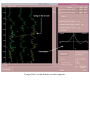
Using the BorNor module of GeoFrame,
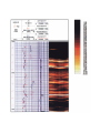
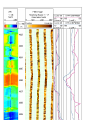
"static" and "dynamic" normalizations of the
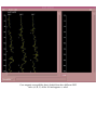
image are applied. In the static normalization,
the resistivity range of the entire interval of
data is computed, and is partitioned into 256
color levels; this image is good for examining
large-scale resistivity variations. In the
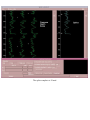
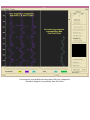
dynamic normalization, the full range of color
levels is assigned to resistivity range of short
intervals (e.g., 2m); thus the color contrast is increased, enhancing the
fine details of the resistivity structure.
Data delivery
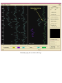
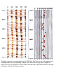
Static images are output as GIF files and added to the on-line database
and the Initial Reports CD-ROM. In the future, dynamic images will be
treated in a similar manner. The FMS data are also saved in DLIS
format and archived.
Once the GHMT logs have been depth shifted, the magnetic polarity
stratigraphy is determined as follows:
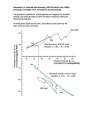
1. The Earth’s main field and the field of the metal drill pipe are
subtracted from the total magnetic field log (MAGB) to isolate
the field anomaly caused by the local formation.
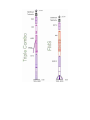
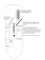
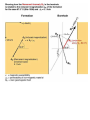
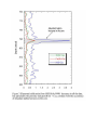
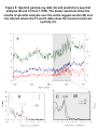
2. The local field anomaly is caused by
the induced and remanent
magnetizations of the local
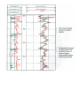
formation (see figure). The induced
anomaly can be calculated from the
magnetic susceptibility log
(MAGS), and so the remanent