Download Grocer 1.0, an Econometric Toolbox for Scilab: a Scilab Point of View

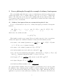
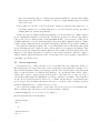
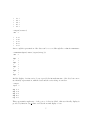
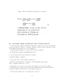
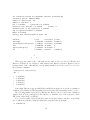
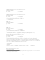
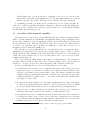
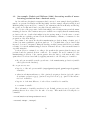
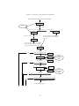
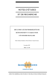
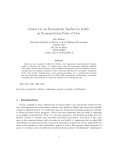
Grocer 1.0, an Econometric Toolbox for Scilab:
a Scilab Point of View∗
Éric Dubois
Direction de la Prévision et de l’Analyse Économique
Télédoc 679
139, rue de Bercy
75012 PARIS
e-mail: [email protected]
Abstract
In his review of Scilab for the Journal of Applied Econometrics, Mrkaic (2001) concludes:
”[...] a dedicated econometric package would significantly increase the appeal of Scilab
to applied econometricians”. Grocer 1.0 (available at http://dubois.ensae.net/grocer.html)
aims at filling this gap and even more. Grocer programming strategy is exposed through the
example of ordinary least squares and the paper shows how the econometrician needs imply a
very different strategy from the one behind Scilab function already performing ordinary least
squares -and much more programming. This paper also presents Grocer main originality with
respect to other econometric software, which consists in a package performing ”automatic”
estimation.
Scilab1 is a matrix-oriented software very similar to Matlab and Gauss, software that are
much used by econometricians. So Scilab should prove very useful to them. In his review of Scilab
for the Journal of Applied Econometrics, Mrkaic (2001) shared this opinion, but concluded:
”[...] a dedicated econometric package would significantly increase the appeal of Scilab to applied
econometricians”. Grocer 1.0 (available at http://dubois.ensae.net/grocer.html) aims at filling
this gap and even more.
Grocer contains most standard econometric procedures. Numerous methods applying to
single equations are available, from ordinary least squares to limited dependent methods through
non linear least squares, instrumental variables estimation... Contrary to the Scilab function
performing ordinary least squares, which is rather rough, each Grocer estimation comes with
a bunch of statistics, standard in econometric applications, such as the Standard Error of the
Regression, the R-squared, Student’s statistics, the Durbin and Watson statistic,... Moreover,
∗
presented at the first Scilab International conference, at INRIA, Rocquencourt, FRANCE, 2004, the 2&3 of
november
1
Available at http://scilabsoft.inria.fr
1
numerous specification tests can be applied to the results of these regressions, such as normality
tests, ARCH tests, Ramsey RESET test, autocorrelation tests, ...
The treatment of non stationary variables, which has now become inescapable when working
with timeseries, can be performed with Grocer. The standard Dickey-Fuller, Phillips and Perron,
KPSS unit root tests are in particular available along with the Engle-Granger and Johansen cointegration methods. Up to date filters (Hodrick-Prescott, Baxter-King or Christiano-Fitzgerald)
have also been implemented.
The treatment of multiple equations models can be done with Grocer. Standard ”oldfashioned” simultaneous equations methods (Zellner Seemingly Unrelated Regressions, two and
three stage least squares) have been implemented along with many up to date VAR methods:
Vector Autoregressions, Vector Error Correction Models, Bayesian Vector Auroregressions. Impulse Response Functions can be calculated and graphed for each of these methods.
For more details about all econometric functions available in Grocer, the interested reader
should refer to Grocer user manual (see Dubois (2004)). The aim of this paper is not however
to provide a comprehensive description of these procedures, but rather to provide an insight
on how they have been implemented in Scilab and present more deeply one of the two features
that make Grocer original with respect to existing econometric packages: an automatic function
that selects the ”best” model from a set of numerous potentially relevant variables, the other,
not presented in the paper, being a set of functions calculating the contributions of exogenous
variables to an endogenous one for any dynamic equation.
Part 1 quickly presents the characteristics of Scilab that makes it attractive to an econometrician. Part 2 illustrates Grocer philosophy through the example of ordinary least squares.
Part 3 presents the automatic function that selects the ”best” model from a set of numerous
potentially relevant variables. Part 4 concludes.
1
Scilab attractiveness for an econometrician
Scilab offers many attractive features for an econometrician. Three of them are particularly
important. First it is free, and therefore portable, a feature that is not guaranteed with any
commercial package, since none of these has become a standard for the profession. Econometricians working on different institutions are therefore not always able to exchange pieces of
works, which they can do with Siclab. Similarly an econometrician using Scilab who changes
her working location will have no problem reusing her programs.
Second, Scilab is very similar to Gauss or Matlab: these software are used a lot by econometricians, in particular those who develop new methods. It is matrix-oriented and contains a
robust numerical optimisation program: econometrics deals basically with matrices and many
econometric problems involve likelihood maximisation. And many programs implementing useful econometric applications written in Gauss or Matlab are available on the web: around half
functions that compose Grocer have been built by translating such programs.
Third, unlike Gauss or Matlab, Scilab allows a user to create her own data types, through
the typed list (tlist) capability: this feature has proved very useful to create the time series type,
of frequent use in a very lively branch of econometrics.
2
2
Grocer philosophy through the example of ordinary least squares
The reader familiar with Scilab may be aware of a Scilab function called leastsq that performs
ordinary least squares. Grocer contains a function, called ols, devoted also to ordinary least
squares. The reader may wonder why bother remaking what already exists in Scilab. The
obvious answer is that ols is not leastsq! To explain why, let us start from what ordinary least
squares are for an econometrician.
2.1
Ordinary least squares from an econometrician point of view
For an econometrician as for anyone else, ordinary least squares perform the following minimisation:
min
(b1 ,...,bn )
T
X
(yt − b1 x1t − . . . − bk xkt ) =
t=1
0
min kY − Xbk2 =
(b1 ,...,bn )
min (Y − Xb) (Y − Xb)
(b1 ,...,bn )
which leads to the well-known result:
0
0
b̂ = (X X)−1 X y
This formula is exactly leastsq’s output. However, from the perspective of an econometrician,
ordinary least squares also entails the calculation of many associated statistics, such as:
• the variance of the estimated parameters: σ̂ 2 =
1
T −k
T
P
t=1
û2t =
1
T −k (Y
0
− X b̂) (Y − X b̂) with:
û = Y − X b̂, the vector of estimated residuals;
0
• the variance of the estimated parameters: V (b̂) = σ̂ 2 (X X)−1 ;
• the Student statistics associated with each coefficient T̂bi =
b̂i
σ̂i ;
• the p-value associated with the hypothesis that a coefficient is nil: p = P |ST −k | > T̂bi /bi = 0 ;
where ST −k designs the Student law with T − k degrees of freedom
P
• the R square: R2 = 1 − PT SCR 2 with ȳ mean of y and SCR = Tt=1 û2t
t=1 (yt −ȳ)
• the adjusted R square: R̄2 = 1 −
SCR
T −k
PT
2
t=1 (yt −ȳ)
T −1
• the Durbin and Watson statistics: DW =
PT
(ût −ût−1 )
t=2
PT
2
t=2 ût
2
ols computes all these statistics. However an applied econometrician’s work does not stop with
the estimation of the coefficients and the calculation of all these statistics. Once the estimation
is done, she should check the validity and robustness of these results. This task involves the
application of specification tests, such as tests of stability of the coefficients (so called Chow test
3
or CUSUM test), tests of homoskedasticty (the most famous of these tests is called the White
test, but there are many other useful tests)... Most of these specification tests imply auxiliary
regressions of the residuals on various exogenous variables. Some tests, such as the CUSUM test
is usually represented graphically.
Lastly, econometricians frequently use data in the form of time series, that is vectors of real
data associated with dates, such as quarterly GDP, monthly inflation,... Therefore many econometric software allow the user to manipulate directly such objects. Important exceptions are
Matlab and Gauss, which do not include or even allow to create, such objects. Grocer function
ols allows to deal with time series, implemented in Grocer through Scilab tlist capability and,
contrary to many software, ols is sufficiently flexible to allow to deal both with matrices and
time series.
2.2
ols architecture
ols architecture, which is summed up in figure 1, derives largely from the objectives previously described:
• the flexibility as regards the authorised inputs obliges to transform them into matrices;
this is done by Grocer functions explox and exploy; both are at the basis of all ”high
level” Grocer functions that are as flexible as ols with respect to the inputs (cf. part 2.4);
• the possibility to apply ols to time series comes trough the creation of a tlist of type
’ts’; this in turn has obliged to write the overloading functions allowing to perform usual
operations with time series, as well as new specific functions useful for the manipulation
of time series (cf. part 2.3);
• there is a ”low-level” function, called ols2, that applies to the objects that appear in the
formula, that is a vector Y and a matrix X;
• further calculations require a lot of intermediate results. For instance, the computation of
some specification tests requires the vector of residuals, the number of variables, the matrix
of exogenous variables, the period of estimation for time series, the names of exogenous
variables,... So, the output of ols function is a tlist, whose type is ’results’: in that case,
the resort to a tlist is just for the sake of collecting all results, without using the overloading
feature associated with tlists;
• the printing of the results is made by a specialised function called prtuniv; this function
takes the results tlist from ols as input; if the results tlist is present in the environment,
then it can be printed again without resorting to a reestimation of the model; as many
Grocer functions that display results on screen, this function uses a very simple function,
called printmat;
• similarly, some results are graphed at the end of an estimation; these graphs are also
obtained by a specialised function, called pltuniv; again, if the results tlist is present
in the environment, then these results can be graphed again without resorting to a reestimation of the model; Scilab graphic functions are used, but they had to be adapted to
4
time series; this is the purpose of function pltseries0 (which also extends Scilab graphic
functions in some directions; for instance, it allows to graph simultaneously series with
curves and bars);
• the results tlist can also be used as an input of many specification tests; again, the corresponding functions are generally built upon a ’low-level’ function and use specialised
printing functions, prtchi and prtfish;
Besides ols, there are numerous functions applying econometric methods to a single equation
model: instrumental variables, least absolute deviations regression, non linear least squares,
logit, probit, tobit, Cochrane-Orcutt ols and maximum likelihood ols regression for AR1 errors,
ols with t-distributed errors, Hoerl-Kennard Ridge Regression, Huber, Ramsay, Andrew or Tukey
robust regression using iteratively reweighted least-squares, Theil-Goldberger mixed estimation.
Beyond their technical specificities, the corresponding functions use basically the same bricks
as ols. All functions can be applied to time series as well as vectors, matrices and strings. They
therefore use also the explox and exploy functions. The results of all these functions are also
displayed by the function prtuniv or graphed by the function pltuniv. And the output of
-almost- all these functions takes the form of a tlist that can be used as input of any function
computing a specification test.
2.3
Grocer time series
As mentioned above, a time series is a vector of real values, associated with dates. In Grocer,
this is implemented as a typed list (tlist). tlists are lists whose first argument is a string vector,
where the first argument of this vector is its type and the other ones the names of the subsequent
fields. So time series have been built as tlists with type ’ts’ and includes three fields: ’freq’,
’dates’ and ’series’. myts(’freq’) is the frequency of the time series: a value of 1 (resp. 4
or 12) indicates that myts is an annual time series (resp. quarterly or monthly - other frequencies
are also allowed). myts(’series’) is the vector of values. myts(’dates’) represents the time
period of myts: they are numerical values to allow more convenience when executing operations
(addition, multiplication,...) on time series (see below).
Grocer function reshape allows to create a time series from a real vector and a starting date.
Take for instance time series myts, created by the following command:
-->myts=reshape([2.1 1.4 3.2 4.5 1.5],’04q1’);
then the fields take the following values:
-->myts(’freq’)
ans =
4.
-->myts(’dates’)
ans =
5
Figure 1: synoptic of the function ols
Input of ols: strings, vectors, matrices, timeseries
explolist
Initial inputs except ‘noprint’
exploy
ts bloc
explouniv
explox
matrices X, Y, names of variables, boolean for the presence of ts in the regression
ols2
a results tlist containing the data, the estimated parameters and the associated statistics
drawx
printmat
prtuniv
pltuniv
pltseries0
drawy
prints results on screen
graphs residuals, fitted values together with true values
a results tlist containing the data, the estimated parameters, the associated statistics, the names of the
variables, the time period if any
prtuniv
pltuniv
prints statistics and p-values
of specification tests
set of specification
tests
statfore
prtchi
(for example)
arlm
prtfish
arlm0
a results tlist containing the ols results tlist, the values of the statistics and their p-values
Legend:
: function
bloc
intermediate results
: name of a Grocer function
output
: output from ols function
: set of Grocer functions
input
: input of ols function
: intermediate results in function ols
other results
: results derived from ols
results
6
!
!
!
!
!
17.
18.
19.
20.
21.
!
!
!
!
!
-->myts(’series’)
ans =
!
!
!
!
!
2.1
1.4
3.2
4.5
1.5
!
!
!
!
!
A more explicit representation of the dates can be recovered through Grocer function num2date:
-->num2date(myts(’dates’),myts(’freq’))
ans =
!4q1
!
!4q2
!
!4q3
!
!4q4
!
!5q1
!
!
!
!
!
!
!
!
!
And the display of a time series does not provide the internal structure of the tlist, but a more
user friendly representation, with the dates and the series facing one another:
-->myts
myts =
4q1
4q2
4q3
4q4
5q1
2.1
1.4
3.2
4.5
1.5
This representation makes use of the power of tlists in Scilab: this user friendly display is
provided by function %ts p, that overloads the normal display of a ts.
7
But, the main interest of using a tlist representation is to be able to define standard operations or functions on tlists: addition, multiplication, division, logarithm,... The corresponding
functions %ts_a_ts, %ts_m_ts, %ts_r_ts, %ts_log... (all in all 27 overloading functions)
have consequently been written. As regards an operation involving two time series (such as the
addition or the multiplication) there is a big difference with the same operation on 2 vectors:
the time series can be of different size, because they do not cover exactly the same time period (provided they have the same frequency: this condition is first tested by the overloading
function); so the overloading function begins by determining the overlapping time period of the
two time series and then performs the operation on the 2 vectors of values restricted to this
overlapping period.
Time series sometimes have NA (Non Available) values. For instance, French macroeconomic
data over the last century do not exist during the 2 world wars: such a series will be NA for the
years 1914-1919 and 1930-1945. So Grocer ts comply with NA values (%nan in Scilab code).
This possibility comes along with some useful flexibility with respect to estimation: the user can
choose a discontinuous estimation period (such as 1920-1939 + 1946-2004) in order to estimate
over periods with non NA values; and, if the user does not specify it, Grocer functions are able
to estimate a time period compatible with the data (more on this below).
A few specific functions have been programmed to lag (function lagts), differentiate (function delts) time series, compute their growth rate (growthr) aggregate monthly time series to
quarterly (m2q) or quarterly to annual (m2a), extrapolate a time series by the value (overlay)
or the growth rate (extrap) of another one...
Lastly, time series can also be created by loading external data through an interface with
Excel.
2.4
The flexibility of econometric functions with respect to inputs and their
implications for the programmer
All high-level econometric functions allow the user to enter various types of data: matrices,
vectors, time series as well as strings. Two kinds of strings are allowed: first, the strings ’const’ or
’cte’2 , that avoids the user to create the constant vector or time series relevant for her problem3 ,
second, the name of an existing variable between quotes. The variable myts presented above can
for instance be entered as such (e.g: ols(myts,’cte’) for the regression of myts on a constant)
or between quotes (ols(’myts’,’cte’)). In the last case Grocer function is able to display the
names of its inputs.
These two characteristics -flexibility and the possibility to keep trace of the names of the
variables- has two major consequences: the constraint it imposes to the programmer and the user
as regards the names of the variables; the need to transform the input variables into matrices
to perform the calculations behind each econometric procedure.
The first consequence results from the fact that, when a variable is entered as a string,
the true variable must be recovered by Scilab command evstr : to recover the ts myts entered
2
The string ’cte’, that is an abbreviation of the French world ’constante’, was first implemented; to maintain
compatibility with earlier versions of Grocer, used by some forerunners, both abbreviations are available in the
1.0 version.
3
Some other usual variables, such as trends, could also be treated this way; this is left for further releases.
8
as ’myts’, you have to run evstr(’myts’). In order to use the good variable, local variables
created before any evstr existing in a Grocer function are prefixed by ’grocer ’ and the user is
recommended not to prefix her variables by ’grocer ’.
The transformation of input variables into matrices is basically done by the two functions
explox and exploy, which are called in function explouniv for all the univariate methods,
which were presented at the end of part 3.2.
These functions perform the following tasks, which imply a battery of conditional operations
and computations:
• determine the type of the input variables;
• for the variables whose type is string, store the string into the vector of names, that will
be used for subsequent display, and thereafter recover the corresponding variables;
• for other types of variables, define the name by a default name provided as an input of
the function (when called from ols or another univariate function, the default name is
’exogenous’) suffixed by the place of the corresponding variable in the list of variables;
• if the user has provided time bounds, then for the variables whose type is time series,
recover the values of the time series over the specified time period;
• if the user has not provided time bounds, then create (for the first encoutered time series)
or update (for the other time series) the admissible time bounds; only when the time
bounds are determined, then recover the values of all time series over the specified time
period;
• if the user has provided the string ’cte’ or ’const’, then the corresponding vector is created
at the end of the program, its size being determined by the size of the other variables in
the regression;
• collect the names of the variables in a vector of names, the corresponding values in a matrix
(Y for exploy and X for explox), define a boolean indicating the presence or absence of
time series in the regression (if there is a time series in the regression, then the bounds of
the regression will be displayed at the end);
2.5
The tlist of results
The arguments of the tlist of results, called say rols, are the following:
• rols(’meth’) = ’ols’ (this is the econometric method: this argument allows a wrapper
function prtres to recognise what display function to use)
• rols(’y’) = y data vector
• rols(’x’) = X data matrix
• rols(’nobs’) = # observations
9
• rols(’nvar’) = # variables
• rols(’beta’) = b̂
• rols(’yhat’) = ŷ
• rols(’resid’) = residuals
• rols(’vcovar’) = estimated variance-covariance matrix of beta
• rols(’sige’) = estimated variance of the residuals
• rols(’sigu’) = sum of squared residuals
• rols(’ser’) = standard error of the regression
• rols(’tstat’) = t-stats
• rols(’pvalue’) = pvalue of the betas
• rols(’dw’) = Durbin-Watson Statistic
• rols(’condindex’) = multicolinearity cond index
• rols(’prescte’) = boolean indicating the presence or absence of a constant in the regression (this boolean is used by the printing function to determinate if the R2 must be
printed or not)
• rols(’rsqr’) = R2
• rols(’rbar’) = R̄2
• rols(’f’) = F-stat for the nullity of coefficients other than the constant
• rols(’pvaluef’) = its significance level
• rols(’prests’) = boolean indicating the presence or absence of a time series in the
regression (this boolean is used by the printing function to determinate if the bounds
must be printed or not)
• rols(’namey’) = name of the y variable
• rols(’namex’) = name of the x variables
• rols(’bounds’) = if there is a time series in the regression, the bounds of the regression
• rols(’like’) = log-likelihood of the regression
10
Figure 2: Hendry and Ericsson (1991) preferred equation
2.6
An example: Hendry and Ericsson (1991) US money demand
In a famous paper, Hendry and Ericsson (1991) have estimated a US money demand that
respected all canons of applied econometrics. Results of their preferred specification as they
were published in their paper are reported in Figure 2.
Retrieving their results in grocer involves the following commands:
-->load(’SCI/macros/grocer/db/bdhenderic.dat’) ;
// load the database that is given with Grocer package
-->bounds(’1964q3’,’1989q2’)
// set the same time bounds as Hendry and Ericsson
-->rhe=ols(’delts(lm1-lp)’,’delts(lp)’,’delts(lagts(1,lm1-lp-ly))’,
’rnet’,’lagts(1,lm1-lp-ly)’,’cte’);
// variables have been entered between quotes: their names are saved for the display;
// variables lm1, lp, ly, rnet are time series: the estimation involves the specific functions
// delts and lagts, as well as the overloaded function %ts_m_ts;
And here is the result of the corresponding Grocer session :
11
ols estimation results for dependent variable: delts(lm1-lp)
estimation period: 1964q3-1989q2
number of observations: 100
number of variables: 5
R^2 = 0.7616185
ajusted R^2 =0.7515814
Overall F test: F(4,95) = 75.880204
p-value = 0
standard error of the regression: 0.0131293
sum of squared residuals: 0.0163761
DW(0) =2.1774376
Belsley, Kuh, Welsch Condition index: 114
variable
delts(lp)
delts(lagts(1,lm1-lp-ly))
rnet
lagts(1,lm1-lp-ly)
cte
coeff
-0.6870384
-0.1746071
-0.6296264
-0.0928556
0.0234367
t-statistic
-5.4783422
-3.0101342
-10.46405
-10.873398
5.818553
p value
3.509D-07
0.0033444
0
0
7.987D-08
*
*
*
When properly rounded, the coefficients are the same as those provided by Hendry and
Ericsson; Student’s T are displayed, while Hendry and Ericsson presented (figures between
brackets under each coefficients) the corresponding standard errors; they can be recovered by
the following commands:
-->rhe(’beta’)./rhe(’tstat’)
ans =
!
!
!
!
!
0.1254099
0.0580064
0.0601704
0.0085397
0.0040279
!
!
!
!
!
Some slight differences appear with Hendry and Ericsson figures; however the re-estimation
of this model by Hendry and Krolzig (2000) leads to the same Student statistics as Grocer ones...
The following statistics presented by Hendry and Ericsson can be found on the estimation
display: their R2 (0.76); their (0.13), called in Grocer ”standard error of the regression”; their
DW (2.18), called in Grocer DW(0).
To recover the results of their specification tests, it is now necessary to run the corresponding
Grocer functions, with the results tlist that has been named rhe as an input:
--> arlm(rhe,4);
12
Lagrange multiplier 1-4 autocorrelation test:
chi2(4)=7.1563181
(p -value
= 0.1278545)
Lagrange multiplier 1-4 autocorrelation test:
F(4,91)=1.941783
(p -value
= 0.1102067)
// this is what Hendry and Ericsson call AR 1-4
--> archz(rhe,4);
ARCH test:
chi2(4)=2.8467913
(p -value
= 0.5837830)
ARCH test:
F(4,87)=0.7357736
(p -value
= 0.5700480)
// this is what Hendry and Ericsson call ARCH 1-4
-->namexbp=rhe(’namex’); bpagan(rhe,namexbp(1:4),namexbp(1:4)+’^2’);
Breusch and Pagan heteroscedasticity test:
F(8,86)=1.3572821
(p -value
= 0.2267534)
// this is what Hendry and Ericsson call Xi2 ; note that the test does not exits as such
// in Grocer, but that it is an example of a more general test called Breusch and Pagan test,
// that has been programmed in Grocer. So Hendry and Ericsson test can be recovered although
// in a more complicated manner than with other tests.4
-->white(rhe)
warning
matrix is close to singular or badly scaled. rcond =
1.0425D-08
White heteroscedasticity test:
chi2(14)=15.475464
4
Writing this article led me to discover 2 slight bugs in the function bpagan: they have been corrected and the
correction posted on Grocer web site.
13
(p -value
= 0.3464440)
White heteroscedasticity test:
F(14,80)=1.0462196
(p -value
= 0.4180710)
// this is what Hendry and Ericsson call Xi Xj
-->reset(rhe,2);
power 2 non linearity RESET test:
F(1,94)=0.0821074
(p -value
= 0.7750922)
// this is what is called by Hendry and Ericsson RESET
-->doornhans(rhe)
Doornik and Hansen normality test:
chi2(2)=1.9768209
(p -value
= 0.3721678)
//This is another, more recent, normality test than the one used by Hendry and Ericsson,
//hence the slightly different numerical results; but the conclusion remains unmodified: at
// standard significance levels, the normality hypothesis is not rejected.
3
The function automatic
An applied econometrician often aims at recovering the economic model that has generated
the data set she has at her disposal: this model is what is called the data generating process.
When a data generating process (DGP) involves a small number of variables among a much
bigger set of potentially important variables, then a researcher who wants to recover the true
model among all the -linear- models than can be built from this data set faces the following
difficulties:
• if she wants to estimate all models that can be built from this data set, then the cost of
search will generally be prohibitive: if there are n variables in the initial set, then there
are 2n potential models;
• if she uses a top-down method based upon the successive elimination, by the mean of a
testing procedure (based for instance on the successive elimination of the variable with the
lowest Student T ), then the number of models to estimate is more limited (at most n), but
the risk of not finding the best model is great; if she chooses a relatively loose significance
level, then she risks retaining erroneous variables, since, as emphasised by Hendry and
14
Krolzig (2000), type I errors are known to accumulate; if she chooses to protect herself
against such a risk with a high significance level, she then risks missing some relevant
variables; and the bigger is the colinearity between variables, the bigger is this risk.
So estimating a relevant econometric model generally involves a lot of time and skill. Recently, Hoover and Perez (1999), with further refinement by Hendry and Krozlig (2000), have
however proposed a computer-based ”general to specific” method to recover with great reliability
the underlying data generating process.
3.1
An outline of the automatic capability
The approach advocated by Hoover-Perez and Hendry-Krolzig consists in exploring a limited
number of paths, starting from each initially non significant variable and performing thereafter
the successive elimination of the less significant variables, provided that the model passes well
chosen specification tests. This approach will lead at the end to a few models, which can then
be chosen by encompassing tests, or if this is not sufficient to obtain only one model, by an
information criterion such as the Akaı̈ke’s one.
The exploration of several paths and the use of specifications tests cover against the risk of
eliminating a relevant variable, but only the more relevant paths are indeed explored. Hendry
and Krozlig Monte Carlo simulations show that this method leads indeed to very satisfactory
results: the average inclusion rate of a non relevant variable can be set at a low level, while
retaining significant power.
The corresponding algorithm, summed up in figure 3, is implemented by Grocer function
automatic, which is (as far as I know) the only econometric package today to provide this very
useful device, except for pc-gets, the commercial package built by Hendry and Krolzig5
From a programming point of view, the following features are noteworthy:
• the function involves several loops or conditional expressions; Scilab relative slowness as
regards these types of operations is certainly a more important drawback than for the
other Grocer programs, but the execution time on a modern computer remains lower than
a minute for the most usual applications; and even if there are loops in this program, most
calculations still involves matrices and so, once again, Scilab philosophy remains rather
well adapted to the problem;
• the function uses many bricks used by other single equations methods: explox and exploy
to transform the input variables into matrices; 5 low-level specification tests for default
use, and potentially all specification tests for a sophisticated user; printing functions;
• a function, the one that performs the specification tests, is itself created in function
automatic; this is made possible by the existence of Scilab instruction deff ;
• the results take the form of a voluminous results tlist, that includes itself other results tlists
(to display the results of stage 0, stage 1 and, if any, stage 2 estimations, it is convenient
to store them as standard estimation results, that take ordinarily the form of tlists); Scilab
flexibility with respect to tlists allows easily such tlist imbrications.
5
Informations about pc-gets are available at http://www.doornik.com/pcgive/pcgets/index.html.
15
3.2
An example: Dubois and Michaux (2004) forecasting models of manufacturing production from a business survey
As done with ols, the function automatic has been tested on an example already published,
namely one presented in Hendry and Krolzig (2000). Another example, taken from Dubois and
Michaux (2004), is presented here: contrary to the estimation taken from Hendry and Krolzig,
the work done for this article has been realised directly with Grocer.
The objective of the paper was to build relationships between business surveys and the manufacturing production. Since business surveys are available more rapidly that the manufacturing
production, the use of such relationships is in fact an important tool in the macroeconomic
exercises that are regularly performed at the French Ministry of Finance, for instance for the
preparation of the State Budget.
Since firms do not assess directly their manufacturing production during a definite period
of time but answer qualitative questions (such as: ”do you think that your production has
increased, decreased or stagnated during the last three months”) many variables are potentially
relevant to forecast the manufacturing production. This made the use of the automatic function
especially attractive.
Seven models were estimated, according to the month in the quarter when the survey was
performed and the quarterly horizon considered. For example, the model estimated for the
manufacturing production of the current quarter when the survey of the first month of the
quarter has been released was built by applying automatic to the following set of variables:
• the endogenous variable was the growth rate of the manufacturing production (variable
called gyman in the database);
the exogenous ones were:
• lags 1 to 3 of the endogenous variable (lagts(gyman),lagts(2,gyman),lagts(3,gyman)):
4 variables;
• values in each first month survey of the opinion about past production (ypa), the opinion
about future production (ppy), opinion about global orders (ccg), opinion on the inventories level: 4 variables;
• lags 0 to 4 of the first difference of each of these 3 variables: 16 variables;
• a constant: 1 variable.
The total number of variables was therefore 24. Default options were used, except for the
printings that are here reduced for the sake of brevity. This entailed the following Grocer
command:
-->load(’SCI/scied/fourgeaud/data2.dat’)
-->bounds(’1979q2’,’2002q4’)
16
Figure 3: synoptic of the function automatic
Input of automatic: strings, vectors, matrices, timeseries
exploy
ts bloc
vector y and its name
separation of the exogenous variables and the options
auto_test
explox
matrix X, its name, bounds (if any)
function called test_func performing
specification tests, names used for their
display
def_results
a results tlist, filled with the first argument
(type of the tlist and names of the following
arguments) and other invariable elements
ols2a
initial model
yes
test if this is the final model
no
auto_stage0
stage0 model
yes
ols1a
test_func
set of
specification
tests
waldf0
test if this is the final model
no
for all non significant variables
ols1a
auto_stage1
test_func
stage 1 models
yes
test if there is one and only one stage 1 model
no
only one
build the union model and calculate the number
of models that are accepted against this model
0 or more than 1
(continued on next page)
17
set of
specification
tests
(stage 2 estimation)
for all non significant variables of the union model
auto_stage1
stage 1 models
yes
test if there is one and only one stage 1 model
no
only one
build the union model and calculate the number
of models that are accepted against this model
0
more than 1
select the union model
select the model according to an
information criterium
THIS
MODEL
IS
THE
FINAL
MODEL
prtauto_univ
printmat
prtuniv
prtauto
prtauto_multi
a results tlist containing the ols results tlists of various estimated model, the way the
final model was obtained, the paths followed in stages 1 and, if any, 2
Legend:
: function
: name of a Grocer function
output
: output from the function
automatic
bloc
: set of Grocer functions
input
: input of the function
automatic
intermediate results
: intermediate results in
the function automatic
instruction
: a intermediate computation in
automatic function
18
-->rman=automatic(’gyman’,’lagts(gyman)’,’lagts(2,gyman)’,’lagts(3,gyman)’,...
-->’ypa_m1’,’ypa_m1-lagts(ypa_m3)’,’lagts(ypa_m3)-lagts(ypa_m2)’,...
-->’lagts(ypa_m2)-lagts(ypa_m1)’,’lagts(ypa_m1)-lagts(2,ypa_m3)’,...
-->’ppy_m1’,’ppy_m1-lagts(ppy_m3)’,’lagts(ppy_m3)-lagts(ppy_m2)’,...
-->’lagts(ppy_m2)-lagts(ppy_m1)’,’lagts(ppy_m1)-lagts(2,ppy_m3)’,...
-->’ccg_m1’,’ccg_m1-lagts(ccg_m3)’,’lagts(ccg_m3)-lagts(ccg_m2)’,...
-->’lagts(ccg_m2)-lagts(ccg_m1)’,’lagts(ccg_m1)-lagts(2,ccg_m3)’,...
-->’sto_m1’,’sto_m1-lagts(sto_m3)’,’lagts(sto_m3)-lagts(sto_m2)’,...
--> ’lagts(sto_m2)-lagts(sto_m1)’,’lagts(sto_m1)-lagts(2,sto_m3)’,...
-->’cte’,’prt=final,test’);
And Grocer results were the following:
__________________________________________________
| results of the automatic regression package
|
__________________________________________________
final model
ending reason: stage 2 models selected by bic criterion
ols estimation results for dependent variable: gyman
estimation period: 1979q2-2002q4
number of observations: 95
number of variables: 4
R^2 = 0.4970310
ajusted R^2 =0.4804496
Overall F test: F(3,91) = 29.975222
p-value = 1.439D-13
standard error of the regression: 0.8614509
sum of squared residuals: 67.530894
DW(0) =2.2836444
Belsley, Kuh, Welsch Condition index: 13
variable
lagts(ccg_m3)-lagts(ccg_m2)
[More (y or n ) ?]
ccg_m1-lagts(ccg_m3)
cte
ppy_m1
coeff
t-statistic p value
0.0845522 2.9341329
0.0042328
0.1103030 4.1064521
0.4862431 5.23963
0.0497842 6.3302334
*
*
*
tests results:
19
0.0000876
0.0000010
9.083D-09
**************
test
test value
Chow pred. fail. (50%) 0.9958242
Chow pred. fail. (90%) 0.8716775
Doornik & Hansen
0.8382420
AR(1-4)
1.233487
hetero x_squared
0.5730995
p-value
0.5069009
0.5538006
0.6576246
0.3026397
0.7507011
*
*
*
The model selected by the algorithm is here the only one that has been displayed, along with
the statistics of the associated specification tests. The display shows however that this model has
been selected among several models whose properties are almost equivalent (ending reason:
stage 2 models selected by bic criterion). It can be worthwhile to print these models.
Since the results have been saved in tlist rman, this can be done by running:
-->prtauto_multi(rman,’stage 2 models’)
which shows all the models (here there only 2) selected at the end of stage 2:
stage 2 models
model #1
ols estimation results for dependent variable: gyman
estimation period: 1979q2-2002q4
number of observations: 95
number of variables: 4
R^2 = 0.4970310
ajusted R^2 =0.4804496
Overall F test: F(3,91) = 29.975222
p-value = 1.439D-13
standard error of the regression: 0.8614509
sum of squared residuals: 67.530894
DW(0) =2.2836444
Belsley, Kuh, Welsch Condition index: 13
variable
lagts(ccg_m3)-lagts(ccg_m2)
ccg_m1-lagts(ccg_m3)
cte
ppy_m1
coeff
0.0845522
0.1103030
0.4862431
0.0497842
t-statistic
2.9341329
4.1064521
5.23963
6.3302334
20
p value
0.0042328
0.0000876
0.0000010
9.083D-09
*
*
*
aic -0.2570812
bic -0.1495495
hq -0.2136303
model #2
ols estimation results for dependent variable: gyman
estimation period: 1979q2-2002q4
number of observations: 95
number of variables: 5
R^2 = 0.5048903
ajusted R^2 =0.4828855
Overall F test: F(4,90) = 22.944477
p-value = 4.332D-13
standard error of the regression: 0.8594292
sum of squared residuals: 66.475665
DW(0) =2.2192735
Belsley, Kuh, Welsch Condition index: 13
variable
lagts(sto_m2)-lagts(sto_m1)
ypa_m1-lagts(ypa_m3)
ccg_m1-lagts(ccg_m3)
cte
ppy_m1
coeff
-0.0757736
0.0524032
0.0998390
0.4926179
0.0503658
t-statistic
-2.1789326
2.2846024
3.6582228
5.3029259
6.4470266
p value
0.0319490
0.0246872
0.0004275
8.081D-07
5.544D-09
*
*
*
aic -0.2517778
bic -0.1173632
hq -0.1974642
*
*
*
As shown in this example, as in many other instances when it has been used at the French
Ministry of Finance, the function automatic has proved a very useful tool for a quick and
21
robust estimation of econometric relationships when a great number of exogenous variables is
potentially relevant.
Conclusion
Grocer is a package that performs most standard econometric methods and some less standard, but very useful ones. Grocer is due to evolve regularly and some new features are already
underway. A few procedures existing in some commercial packages and some more rare but
nevertheless useful methods (notably in the bayesian field) remain to be implemented. The
matrix-oriented nature of Scilab will make it easy to stay at the forefront of the econometric
science. And the great similarity between Scilab and Matlab or Gauss will help as well.
Acknowledgements
I wish to thank the Scilab team for their precious advices, James Le Sage for having provided
the basis of so many grocer functions, Emmanuel Michaux for his faithful use and testing of
Grocer, Catherine Dubois, Benoı̂t Bellone and Alexandre Espinoza for their careful reading and
useful comments on this article.
22
References
É. Dubois (2004): ”Grocer 1.0: An Econometric Toolbox For Scilab”, user manual, available at
http://dubois.ensae.net/grocer.html.
É. Dubois and E. Michaux (2004): ”Étalonnages à l’aide d’enquêtes de conjoncture : de nouveaux
résultats”, forthcoming in Économie et Prévision, available at http://dubois.ensae.net/papers.html.
D.F Hendry et N.R Ericsson (1991): ”Modelling the demand for narrow money in the United
Kingdom and the United States”’, European Economic Review, pp. 833-886.
D.F. Hendry and H-M Krozlig (1999): ”Improving on ’data mining reconsidered’ by K.D. Hoover
and S.J. Perez ”, Econometrics Journal, n◦ 2, pp. 41-58.
D.F. Hendry and H-M Krozlig (2000): ”Computer Automation of General-to-Specific Model Selection Procedures”, Journal of Economic Dynamics and Control, 25(6-7), pp. 831-866.
K.D Hoover and S.J. Perez (1999): ”Data mining reconsidered: a general to specific approach to
specification search”, Econometrics Journal, n◦ 2, pp. 167-191.
M. Mrkaic (2001): ”Scilab as an Econometric Programming System”, Journal of Applied Econometrics,
vol. 16, n◦ 4, July-August, pp. 553-559.
23