1
David Fernández
Development of the calibration and limit checking
modules for a satellite’s ground control software
Aalto Universiy School of Electrical Engineering
Department of Radio Science and Engineering
Thesis submitted for examination for the degree of Master of Science in Technology.
Otaniemi, Espoo, 31.08.2013
Thesis supervisor and instructor: D.Sc. (Tech.) Jaan Praks
Aalto University
School of Electrical Engineering
Abstract of the
Final Project
Author: David Fernández
Title: Development of the calibration and limit checking modules for a satellite’s
ground control software
Date: 31.08.2013
Language: English
School of Electrical Engineering
Deparment of Radio Science and Engineering
Professorship: Space Technology
Number of pages: 71
Code: S-92
Supervisor: D.Sc. (Tech.) Jaan Praks
The goal of this project is to develop the calibration and limit checking modules
for Hummingbird, an open source software platform for controlling ground
stations and satellites which is being developed by CGI Group Inc. in cooperation with the University of Tartu. Hummingbird is presented in detail
and its architecture, functionalities and core technologies are described in the work.
The work also gives a short overview of the topics which are most relevant to
satellite communications. Such as orbits, communication protocols, the ground
segment and ground segment software solutions.
The software design made in this work was developed in close cooperation with
the scientists working on the Estonian student satellite. The result is a completely
configurable software prepared to be fully integrated with Hummingbird when
necessary.
Keywords: nanosatellite, ground station, calibration, limits, communications,
orbits, Hummingbird
All our dreams can come true, if we have the courage to pursue
them.
Walt Disney
Licence
CC0 3.0 Unported (CC0 3.0)
Attribution-ShareAlike
You
•
•
•
are free:
to copy, distribute, display and perform the work
to make derivative works
to make commercial use of the work
Under the following conditions:
• Attribution — You must give the original author credit.
• Share Alike — If you alter, transform, or build upon this
work, you may distribute the resulting work only under a
licence identical to this one.
With the understanding that:
• Waiver — Any of the above conditions can be waived if
you get permission from the copyright holder.
• Public Domain — Where the work or any of its elements
is in the public domain under applicable law, that status
is in no way affected by the licence.
• Other Rights — In no way are any of the following rights
affected by the licence:
– Your fair dealing or fair use rights, or other applicable
copyright exceptions and limitations;
– The author’s moral righs;
– Rights other persons may have either in the work itself
or in how the work is used, such as publicity or privacy
rights.
Notice — For any reuse or distribution, you must make clear to
others the licence terms of this work.
This is a human-readable summary of the Legal Code:
http://creativecommons.org/licenses/by-sa/3.0/legalcode
Note: this licence does not apply to the following parts of the thesis: Figure 1.1,
Figure 1.2, Figure 1.3, Figure 1.4, Figure 1.5, Figure 2.3, Figure 2.6 and images
on Table 2.1. The copyright belongs to their respective authors.
Preface
Before I started this thesis, my knowledge about space technology was close to
zero. Nevertheless, when I was told about the possibility of working in the project
of building the first satellite that Finland will launch into space, I did not hesitate
for a second. Working in the project was great opportunity and I had to take it.
My work has been done at the Department of Radio Science and Engineering of
Aalto University and my main goal has been to produce software for the ground
segment of the mission. It has been really challenging, but it has also given me
the chance to gain knowledge in several space related areas which some months
ago where somehow like magic for me.
It has been real pleasure being a small part of this project. I believe these satellites
are the present and future for universities, and they can help students see that all
the effort they put during their studies can accomplish something as amazing as
putting their own satellite into orbit.
v
Acknowledgements
I cannot start in any other way than thanking my parents, Manuel and María del
Carmen. Without you this would not be happening, thank you for your constant
love and trust. Thank you for everything you have taught me and keep teaching
me everyday. Also, thank you for your great support when I decided to move
abroad. I love you.
Thanks to Aalto University, especially to Jaan Praks, who invited me to participate in the great adventure that is Aalto-1 and has supervised my thesis. Also,
many thanks to the Aalto-1 team. It has been great working with you.
Many thanks to Urmas Kvell and the ESTCube team. Thank you for your cooperation during my visits to Estonia and also for your invitation to stay at the
Tõravere Observatory for two weeks. My stay there was very fruitful and interesting.
I would also like to thank Gonzalo Mariscal, International Manager of the School
of Engineering at Universidad Europea de Madrid. Thank you for your support
during these two years and also for all the times I bothered you with questions
before I moved to Finland.
Finally, I want to say thanks to all the friends who have helped me since I came
to the country; especially to Adrián Yanes, who convinced me to come to Finland
in the first place and has been a great friend for the last eight years. Also to Borja
Tarrasó, whose support and friendship since I arrived have been very important
to me. You guys have always been there, thanks. I do not want to forget Alberto
Alonso, one of the last additions to our group whom has proved to be a great
friend. Last, but not least, I want to thank Tuomo Ryynänen and his family. You
have made me feel very welcomed in your country. I hope that, in the future, I
will be able to reciprocate in mine.
Otaniemi, Espoo, August 2013.
David.
vi
Contents
1 Introduction
1.1 Background . . . . . . .
1.1.1 Aalto-1 . . . . .
1.1.2 ESTCube-1 . . .
1.2 Problem statement . . .
1.3 Research objectives and
1.4 Motivations . . . . . . .
1.5 Outline of the thesis . .
.
.
.
.
.
.
.
.
.
.
.
.
.
.
.
.
.
.
.
.
.
.
.
.
.
.
.
.
.
.
.
.
.
.
.
.
.
.
.
.
.
.
.
.
.
.
.
.
.
.
.
.
.
.
.
.
.
.
.
.
.
.
.
.
.
.
.
.
.
.
.
.
.
.
.
.
.
.
.
.
.
.
.
.
.
.
.
.
.
.
.
.
.
.
.
.
.
.
.
.
.
.
.
.
.
.
.
.
.
.
.
.
.
.
.
.
.
.
.
.
.
.
.
.
.
.
.
.
.
.
.
.
.
.
.
.
.
.
.
.
.
.
.
.
.
.
.
.
.
.
.
.
.
.
1
4
4
5
6
7
7
8
2 Satellite Communications
2.1 Orbits . . . . . . . . . . . . . . . .
2.1.1 Kepler’s Laws . . . . . . .
2.1.2 Classical Orbital Elements
2.1.3 Ground Tracks . . . . . . .
2.1.4 Two-Line Elements . . . .
2.2 Data . . . . . . . . . . . . . . . . .
2.2.1 Beacon . . . . . . . . . . .
2.2.2 Telemetry . . . . . . . . . .
2.2.3 Telecommands . . . . . . .
2.3 Ground Station . . . . . . . . . . .
2.3.1 Ground station hardware .
2.3.2 Software . . . . . . . . . . .
2.3.3 Protocols . . . . . . . . . .
.
.
.
.
.
.
.
.
.
.
.
.
.
.
.
.
.
.
.
.
.
.
.
.
.
.
.
.
.
.
.
.
.
.
.
.
.
.
.
.
.
.
.
.
.
.
.
.
.
.
.
.
.
.
.
.
.
.
.
.
.
.
.
.
.
.
.
.
.
.
.
.
.
.
.
.
.
.
.
.
.
.
.
.
.
.
.
.
.
.
.
.
.
.
.
.
.
.
.
.
.
.
.
.
.
.
.
.
.
.
.
.
.
.
.
.
.
.
.
.
.
.
.
.
.
.
.
.
.
.
.
.
.
.
.
.
.
.
.
.
.
.
.
.
.
.
.
.
.
.
.
.
.
.
.
.
.
.
.
.
.
.
.
.
.
.
.
.
.
.
.
.
.
.
.
.
.
.
.
.
.
.
.
.
.
.
.
.
.
.
.
.
.
.
.
.
.
.
.
.
.
.
.
.
.
.
.
.
.
.
.
.
.
.
.
.
.
.
.
.
.
.
.
.
.
.
.
.
.
.
.
.
.
.
.
.
.
.
.
.
.
.
.
.
.
.
.
.
.
.
.
.
.
.
.
.
.
.
.
.
.
.
.
.
.
.
.
.
.
.
.
.
.
9
9
9
10
13
14
15
15
15
17
17
19
19
20
3 Hummingbird: the open
controlling remote assets
3.1 Overview . . . . . . . . .
3.2 Functionalities . . . . .
3.3 Architecture . . . . . . .
. . . .
. . . .
. . . .
. . . .
scope
. . . .
. . . .
.
.
.
.
.
.
.
source platform for monitoring and
23
. . . . . . . . . . . . . . . . . . . . . . . . . . . 23
. . . . . . . . . . . . . . . . . . . . . . . . . . . 24
. . . . . . . . . . . . . . . . . . . . . . . . . . . 24
4 Requirements
4.1 Common information for both modules
4.1.1 General Description . . . . . . . .
4.1.2 External Interface Requirements
4.1.3 Non-Functional Requirements . .
4.2 Calibration module . . . . . . . . . . . . .
.
.
.
.
.
.
.
.
.
.
.
.
.
.
.
.
.
.
.
.
.
.
.
.
.
.
.
.
.
.
.
.
.
.
.
.
.
.
.
.
.
.
.
.
.
.
.
.
.
.
.
.
.
.
.
.
.
.
.
.
.
.
.
.
.
.
.
.
.
.
.
.
.
.
.
.
.
.
.
.
.
.
.
.
.
25
25
25
26
26
27
CONTENTS
4.3
4.2.1
4.2.2
4.2.3
4.2.4
4.2.5
Limit
4.3.1
4.3.2
4.3.3
4.3.4
4.3.5
Introduction . . . . . . . . . . . .
General Description . . . . . . . .
External Interface Requirements
Functional Requirements . . . . .
Non-Functional Requirements . .
checking module . . . . . . . . . .
Introduction . . . . . . . . . . . .
General Description . . . . . . . .
External Interface Requirements
Functional Requirements . . . . .
Non-Functional Requirements . .
.
.
.
.
.
.
.
.
.
.
.
.
.
.
.
.
.
.
.
.
.
.
.
.
.
.
.
.
.
.
.
.
.
5 Implementation
5.1 Technologies used . . . . . . . . . . . . . . . .
5.2 Implementation of the calibration module . .
5.2.1 Camel Integration . . . . . . . . . . . .
5.2.2 Loading the calibration information .
5.2.3 Calibration . . . . . . . . . . . . . . . .
5.3 Implementation of the limit checking module
5.3.1 Camel integration . . . . . . . . . . . .
5.3.2 Loading the limits information . . . .
5.3.3 Limit checking . . . . . . . . . . . . . .
.
.
.
.
.
.
.
.
.
.
.
.
.
.
.
.
.
.
.
.
.
.
.
.
.
.
.
.
.
.
.
.
.
.
.
.
.
.
.
.
.
.
.
.
.
.
.
.
.
.
.
.
.
.
.
.
.
.
.
.
.
.
.
.
.
.
.
.
.
.
.
.
.
.
.
.
.
.
.
.
.
.
.
.
.
.
.
.
.
.
.
.
.
.
.
.
.
.
.
.
.
.
.
.
.
.
.
.
.
.
.
.
.
.
.
.
.
.
.
.
.
.
.
.
.
.
.
.
.
.
.
.
.
.
.
.
.
.
.
.
.
.
.
.
.
.
.
.
.
.
.
.
.
.
.
.
.
.
.
.
.
.
.
.
.
.
.
.
.
.
.
.
.
.
.
.
.
.
.
.
.
.
.
.
.
.
.
.
.
.
.
.
.
.
.
.
.
.
.
.
.
.
.
.
.
.
.
.
.
.
.
.
.
.
.
.
.
.
.
.
.
.
.
.
.
.
.
.
.
.
.
.
.
.
.
.
.
.
.
.
.
.
.
.
.
.
.
.
.
.
.
.
.
.
.
.
.
.
.
.
6 User manual
6.1 Calibration module . . . . . . . . . . . . . . . . . . . . . . . . . . . . .
6.1.1 Structure of the XML file . . . . . . . . . . . . . . . . . . . .
6.1.2 Example of simple calibration . . . . . . . . . . . . . . . . . .
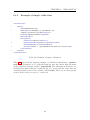
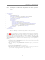
6.1.3 Example of calibration dependent on other parameters . . .
6.1.4 Example of calibration dependent on other parameters which
are dependent on others . . . . . . . . . . . . . . . . . . . . .
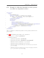
6.1.5 Example of the result of the calibration being a vector . . .
6.2 Limit checking module . . . . . . . . . . . . . . . . . . . . . . . . . .
6.2.1 Example of configuration with sanity limits . . . . . . . . .
6.2.2 Example of configuration without sanity limits . . . . . . .
.
.
.
.
.
.
.
.
.
.
.
27
27
28
29
31
31
31
31
34
34
36
.
.
.
.
.
.
.
.
.
37
37
38
38
42
46
50
51
53
56
.
.
.
.
58
58
59
60
61
.
.
.
.
.
62
63
63
65
65
7 Conclussions
66
8 Future work
68
Bibliography
69
viii
List of Figures
Figure 1.1 – Sputnik 1, first artificial satellite launched by the Soviet
Union in 1957 (National Aeronautics and Space Administration Public Domain) . . . . . . . . . . . . . . . . . . . . . . . . . . . . .
Figure 1.2 – Explorer 1, first artificial satellite launched by the United
States in 1958 (National Aeronautics and Space Administration Public Domain) . . . . . . . . . . . . . . . . . . . . . . . . . . . . .
Figure 1.3 – Satellite Mass and Cost Classification [3] . . . . . . . . . . .
Figure 1.4 – Artist’s view of the Aalto-1 satellite . . . . . . . . . . . . . .
Figure 1.5 – Artist’s view of the ESTCube-1 satellite . . . . . . . . . . .
.
2
.
.
.
.
2
4
4
5
Figure 2.1 – Semimajor axis on an ellipse . . . . . . . . . . . . . . . . . . .
Figure 2.2 – Shapes of an orbit based on its eccentricity . . . . . . . . . .
Figure 2.3 – Classical Orbital Elements [12] . . . . . . . . . . . . . . . . . .
Figure 2.4 – Ground Tracks of ESTCube-1 . . . . . . . . . . . . . . . . . .
Figure 2.5 – Telemetry user interface of the ground station software of
the satellite MaSat-1 . . . . . . . . . . . . . . . . . . . . . . . . . . .
Figure 2.6 – Picture of South Africa taken from the nanosatellite MaSat-1
Figure 2.7 – Diagram of a ground station . . . . . . . . . . . . . . . . . . .
Figure 2.8 – AX.25 Supervisory and Unnumbered frames [23] . . . . . . .
Figure 2.9 – AX.25 Information frame [23] . . . . . . . . . . . . . . . . . . .
Figure 2.10– FX.25 frame structure [24] . . . . . . . . . . . . . . . . . . . .
10
11
12
13
16
16
18
21
22
22
Figure 4.1 – Limit checker with sanity limits available . . . . . . . . . . . . 32
Figure 4.2 – Limit checker only with soft and hard limits . . . . . . . . . . 33
Figure 5.1 – Class diagram of the Camel integration . . . . . . . . . . . . .
Figure 5.2 – Diagram of the classes involved in loading the calibration
information onto the system . . . . . . . . . . . . . . . . . . . . . . .
Figure 5.3 – Sequence diagram which represents the interactions between
the different classes present when loading the calibration information
Figure 5.4 – Diagram representing the classes involved in the calibration
process . . . . . . . . . . . . . . . . . . . . . . . . . . . . . . . . . . . .
Figure 5.5 – Flow chart of the algorithm to manage incoming parameters
in the calibration module . . . . . . . . . . . . . . . . . . . . . . . . .
Figure 5.6 – Sequence diagram describing the interactions between the
different classes when managing incoming parameters in the calibration module . . . . . . . . . . . . . . . . . . . . . . . . . . . . . . .
Figure 5.7 – Class diagram of the Camel integration . . . . . . . . . . . . .
ix
39
43
44
47
48
49
51
LIST OF FIGURES
Figure 5.8 – Diagram of the classes involved in loading the limits information onto the system . . . . . . . . . . . . . . . . . . . . . . . . .
Figure 5.9 – Sequence diagram which represents the interactions between
the different classes present when loading the limits information
Figure 5.10– Diagram representing the classes involved in the limit checking process . . . . . . . . . . . . . . . . . . . . . . . . . . . . . . . .
Figure 5.11– Diagram representing the classes involved in the limit checking process . . . . . . . . . . . . . . . . . . . . . . . . . . . . . . . .
Figure 5.12– Diagram representing the classes involved in the limit checking process . . . . . . . . . . . . . . . . . . . . . . . . . . . . . . . .
x
. 53
. 54
. 56
. 57
. 57
List of Tables
Table 2.1 – Types of orbits and their inclination [12] . . . . . . . . . . . .
Table 2.2 – NASA’s classification of orbits [13] . . . . . . . . . . . . . . .
Table 2.3 – Two-Line Element set format definition, Line 1 . . . . . . . .
Table 2.4 – Two-Line Element set format definition, Line 2 . . . . . . . .
Table 2.5 – Common radio frequencies used for amateur satellite communications . . . . . . . . . . . . . . . . . . . . . . . . . . . . . . . .
Table 2.6 – OSI Model [22] . . . . . . . . . . . . . . . . . . . . . . . . . . .
.
.
.
.
Table 5.1 – Camel integration Java code for the calibrator . . . . . . . .
Table 5.2 – Java code showing the Camel integration of ParameterProcessor . . . . . . . . . . . . . . . . . . . . . . . . . . . . . . . . . . .
Table 5.3 – Java code used to evaluate a script with BeanShell . . . . .
Table 5.4 – Java code used to retrieve the information from the interpreter
and generate the new parameters . . . . . . . . . . . . . . . . . . .
Table 5.5 – Camel integration Java code for the limit checker . . . . . .
. 40
Table 6.1 – Structure of the XML file used to configure the calibrators .
Table 6.2 – Example of simple calibration . . . . . . . . . . . . . . . . . .
Table 6.3 – Example of calibration dependent on other parameters . . .
Table 6.4 – Example of calibration dependent on other parameters which
also depend on others . . . . . . . . . . . . . . . . . . . . . . . . . .
Table 6.5 – Example of calibration which returns a vector as result . . .
Table 6.6 – Structure of the XML file used to configure the limits . . . .
Table 6.7 – Limit checking with sanity limits . . . . . . . . . . . . . . . .
Table 6.8 – Limit checking without sanity limits . . . . . . . . . . . . . .
xi
12
13
14
15
. 19
. 21
. 41
. 49
. 50
. 52
. 59
. 60
. 61
.
.
.
.
.
62
63
64
65
65
Symbols and Acronyms
Symbols
a
e
i
Ω
ω
υ
Semimajor axis
Eccentricity
Inclination
Right ascension of the ascending node
Argument of the perigee
True anomaly
xii
LIST OF TABLES
Acronyms
Aalto-1
AX.25
COE
CubeSat
ESA
E-sail
ESTCube-1
Explorer 1
FMI
GUI
GENSO
GS
GSO
HEO
Hummingbird
Inmarsat-4
ISS
JMS
JRE
JVM
LEO
MaSat-1
MEO
NaN
NASA
NORAD
OpenGL
OSI
OSGI
RADMON
Sputnik 1
TLE
UHF
VHF
XML
First nano-satellite being built by Aalto University (Espoo, Finland)
Data link layer protocol
Classical Orbital Elements
Standard for nanosatellites
European Space Agency
Electric Solar Wind Sail
First Estonian satellite
First artificial satellite launched by the United States
Finnish Meteorological Institute
Graphical User Interface
Global Education Network for Satellite Operations
Ground Station
Geosynchronous Orbit
High Earth Orbit
Open source platform for monitoring and controlling remote assets
Communications satellite operated the satellite operator Inmarsat
International Space Station
Java Message Service
Java Runtime Environment
Java Virtual Machine
Low Earth Orbit
First Hungarian satellite
Medium Earth Orbit
Not a Number
National Aeronautics and Space Administration
North American Aerospace Defense Command
Open Graphics Library
Open Systems Interconnection
Open Services Gateway Initiative
Radiation Monitor, payload of Aalto-1
First artificial satellite launched by the Soviet Union
Two-Line Elements
Ultra High Frequency
Very High Frequency
Extensible Markup Language
xiii
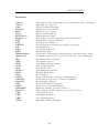
Chapter 1
Introduction
The relationship between human beings and space has existed since the beginning
of time. Space has always been a source of mystery, something we want to understand. More than 4000 years ago, based on the movements of the Sun and the
planets, the Egyptians and the Babylonians developed calendars for growing their
crops. Later, the ancient Greeks introduced the concept of astronomy, the science
of the heavens. Other examples are philosophers such as Nicolaus Copernicus,
Johannes Kepler, who explained the motion of the planets, and Galileo Galilei,
who has been called the "father of modern observational astronomy" [1]. In the
17th century, Sir Isaac Newton invented calculus, developed his law of gravitation
and performed important experiments in optics.
The technological advancements of the 20th century, specially accelerated by the
World War II, made physical exploration of space become possible. This exploration is mainly carried out by the use of satellites. A satellite is a natural or
artificial object moving around a celestial body. This motion is described as an
orbit, defined by the dominant force of gravity from the bigger body. In early 1945,
the United States started the Vanguard Rocket development to launch a satellite.
However, after several failed launches, it was the Soviet Union who took the advantage by launching the Sputnik-1 (Figure 1.1) on October 4, 1957. Finally, on
January 31, 1958 the United States managed to launch their first artificial satellite,
the Explorer-1 (Figure 1.2). During the Cold War, the space race between the two
superpowers was a hard fight which made space technology advance quite rapidly.
1
CHAPTER 1. INTRODUCTION
Figure 1.1: Sputnik 1, first artificial satellite launched by the Soviet Union in 1957
(National Aeronautics and Space Administration - Public Domain)
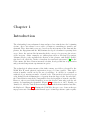
Figure 1.2: Explorer 1, first artificial satellite launched by the United States in
1958 (National Aeronautics and Space Administration - Public Domain)
2
CHAPTER 1. INTRODUCTION
As of October 1, 2011 there were 966 operating satellites in orbit. About two-thirds
of these were owned by the United States, Russia and China [2]. The satellites
can be divided into four main categories according to their usage:
• Communications satellites: used for television, radio, Internet and telephone
services.
• Navigation satellites: using radio time signals, these satellites allow mobile
receivers on the ground to determine their exact position. They are also used
to determine the location of satellites situated in lower orbits.
• Exploration satellites: used to observe distant planets, galaxies and other
outer space objects by using telescopes and other sensors.
• Remote sensing satellites: Remote sensing satellites are used to gather information about the nature and condition of Earth. The sensors in this kind
of satellites receive electromagnetic emissions in several spectral bands and
can detect, amongst others, the object’s composition and temperature, environmental conditions. This type of satellites have sometimes also been used
for military surveillance.
The constant evolution of technology and the growth of human needs have made
the complexity and size of the satellites grow throughout the last decades. Satellite mass has grown from Sputnik’s 84 kg and Explorer-1’s 14k kg to Inmarsat-4’s
almost 6,000 kg in 2008 [3]. The main consequence of this, amongst others, has
been an increment in mission costs.
To counter this trend, the small satellite movement was created by the academic
community and it has shown how mission costs can be cut dramatically to a point
in which a university can build and launch their own satellite. (Figure 1.3). The
success of this concept has created a vigorous industry. Aalto University’s student
satellite Aalto-1 and Estonian student satellite ESTCube-1, projects with which
this thesis is related to, are nanosatellites, and the perfect example of this new
trend.
3
CHAPTER 1. INTRODUCTION
Figure 1.3: Satellite Mass and Cost Classification [3]
1.1
Background
This thesis is closely related to two different university based nanosatellite projects,
Aalto-1 and ESTCube-1. These two projects are based on the most common
standard used by university satellites: CubeSat [4], an open standard developed
by the California Polytechnic State University and Stanford University.
1.1.1
Aalto-1
Led by Aalto University, Aalto-1 project aims to build a multi-payload remote
sensing nanosatellite (Figure 1.4). The size of the satellite is approximately 34 cm
x 10 cm x 10 cm with a mass of less than 4 kg [5]. Aalto-1 also intents to be the
first Finnish satellite.
Figure 1.4: Artist’s view of the Aalto-1 satellite
4
CHAPTER 1. INTRODUCTION
There are different institutions cooperating to make this possible. The main payload, the imaging spectrometer, has been designed and built by VTT Technical
Research Centre of Finland. The Radiation Monitor (RADMON) has been designed by the Universities of Helsinki and Turku in cooperation with the Finnish
Meteorological Institute (FMI). The Plasma Brake has been designed by a consortium including the FMI, the Department of Physics of the University of Helsinki,
the Departments of Physics and Astronomy and Information Technology of the
University of Turku, the Accelerator laboratory of the University of Jyväskylä,
Aboa Space Resarch Oy, Oxford Instruments Oy and other Finnish companies.
Meanwhile, Aalto University is responsible for designing and building the satellite
platform and the day-to-day operation of the project. [6]
Aalto-1’s mission is to demonstrate the technologies of the payloads in space environment and measure their performance. In addition, it is also an educational
project. Students are the main workforce towards its success. Being the the first
Finnish student satellite mission, is a good tool to improve Finnish space teaching
and also allow students to be in touch with prominent partners, both domestic
and international, in the space technology field.
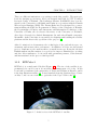
1.1.2
ESTCube-1
ESTCube-1 is a single-unit CubeSat (Figure 1.5). The size of the satellite is approximately 10 cm x 10 cm x 10 cm with a maximum mass of 1.33 kg. It has
been built by students of the universities of Tartu and Tallinn, in Estonia, and it
is the first Estonian satellite [8]. It was launched from the Guaiana Space Centre
on May 7, 2013 as one of the three payloads of the Vega VV02 rocket [9].
Figure 1.5: Artist’s view of the ESTCube-1 satellite
5
CHAPTER 1. INTRODUCTION
ESTCube-1’s main goal is to observe and measure the E-sail [7] effect for the first
time. It has been placed into a polar low Earth orbit (LEO) and will deploy a single
10 m long and 9 mm wide tether [8]. This is related to Aalto-1’s Plasma Brake,
which will deploy a 100 m long tether. The required duration of ESTCube-1’s
mission is a few weeks and it can be extended to about a year.
1.2
Problem statement
Any satellite mission is divided in two segments:
• Space segment: the satellite.
• Ground segment: this segment provides the means and resources to manage
and control the data produced by the diverse instruments [10].
The main part of the groud segment is the ground station. It is the first and final
point of communication with the satellite, the place where the data is received and
where the satellite is controlled from.
One of the main tasks of any mission is analysing the information received from
its several sensors. However, the values generated by the sensors are not usually
valid for scientific use as they are received, they are digital values which are not
presented in any particular units and need to be calibrated.
The calibration process generates useful scientific values from those generated by
the sensors. The equations to do so are provided by the vendors or calculated
by experimentation before the launch. One of the main reasons for calibrating
the values once they have been received by the ground station is saving downlink
bandwidth. For example, a parameter C can be calculated based on the values of
A and B, so it makes no sense to calculate it on board and waste downlink bandwidth to send C, when it can be done on the ground. In addition, the calibration
equations might change over time, and it is much simpler to change something on
the ground segment software than on the satellite.
The received values also need to be checked to see if they are within the specified
limits. This allows scientists to discard invalid values or see how healthy the
systems in the satellite are. These comparisons will generate several responses in
the ground software, so again it only makes sense to do it on the ground.
6
CHAPTER 1. INTRODUCTION
1.3
Research objectives and scope
The purpose of this thesis is to develop the calibration and limit checking modules
for a ground control software which will solve the problems mentioned earlier.
Using ESTCube-1 project as a baseline, the author aims to develop such systems
which are generic enough to be used by any number of satellite missions. The
modules developed will be integrated into Hummingbird, an open source platform
for monitoring and controlling remote assets, which will be explained later in this
work.
The following items support this purpose:
• Research about satellite orbits and how they affect satellite-Earth communications.
• Research about what types data are exchanged between satellites and ground
stations.
• See what are the different parts of a ground station, including hardware and
software pieces.
• Present the most common protocols used for amateur satellite communications.
1.4
Motivations
When the moment came to choose a software solution for Aalto-1’s ground station,
the approach was to develop something ad-hoc for the mission. There was no
available software which was good enough for the mission’s requirements unless it
was oriented for big professional satellites. However, due to the cooperation with
the University of Tartu, Hummingbird came into play as a real strong option. It
is an open source project which, in addition to controlling the ground station and
satellite, also aims to create a network of ground stations around the world.
The development of this product will not only benefit both, Aalto University and
the University of Tartu. Being open source, any mission can have a ready-to-use,
fully tested software as a baseline for their ground control systems, which will help
small satellite missions shorten their development time frames.
7
CHAPTER 1. INTRODUCTION
1.5
Outline of the thesis
This thesis is structured as follows: the second chapter gives a general overview
about satellite communications, how orbits affect them, what data is transmitted,
what the different protocols are and which hardware and software components
are used to carry out those communications. The third chapter explains briefly
what Hummingbird is and what is behind it. The fourth chapter goes through
the requirements set for the software project whereas the fifth one focuses on the
design and implementation. Chapter six comprises a short user manual. Chapter
seven summarizes the conclusions of this thesis. Finally, chapter eight explains
what the next steps in the project are.
8
Chapter 2
Satellite Communications
In order to understand how the satellites communicate with Earth, the very basics
of satellite communications are covered in this chapter. The first section describes
what orbits are, how they are described and how that information can be delivered by a computer. Afterwards, the types of different data exchanged by the
satellite and the ground station will be covered. The last section of the chapter
presents what a ground station is, its hardware and software components and how
it communicates with a satellite in space.
2.1
Orbits
An orbit is the gravitationally curved path of an object around a center of
mass. Examples of orbits can be the Earth around the Sun or artificial satellites
around the Earth.
2.1.1
Kepler’s Laws
Planetary movements were first mathematically defined by the German mathematician, astronomer and astrologer Johannes Kepler in the 17th century. He
concentrated his observations into three simple laws [11]:
• The orbit of each planet is an ellipse with the Sun occupying one focus.
• The line joining the Sun to a planet sweeps out equal areas in equal intervals
of time.
• A planet’s orbital period is proportional to the mean distance between the
Sun and the planet, raised to the power of 3/2.
These laws generally apply to every celestial body. When analysing the movement
of two bodies, if one is much bigger than the other, an approximation known as
9
CHAPTER 2. SATELLITE COMMUNICATIONS
the two-body problem can be used. It assumes that both bodies are spherical and
they are modelled as if they were point particles. This means that influences from
any third body are discarded. The solution of the two-body problem states that
the smaller body orbits around the bigger one in an elliptical orbit which can be
described by six parameters. These parameters will be explained in detail in the
next section.
2.1.2
Classical Orbital Elements
The Classical Orbital Elements (COEs) are six parameters which uniquely define
the orbit and location of the body. They also can be used to predict future positions
of the satellite. [12]
The first two elements, the orbit’s size and shape are defined based on a 2D
representation on an ellipse (Figure 2.1).
Figure 2.1: Semimajor axis on an ellipse
• The semimajor axis (a) is one half the distance across the long axis of the
orbit, and it represents the orbit’s size.
• The eccentricity (e) represents the shape of the orbit. It describes how much
the ellipse is elongated compared to a circle. Based on the latter, the orbit
can have different shapes, as shown in Figure 2.2.
10
CHAPTER 2. SATELLITE COMMUNICATIONS
Figure 2.2: Shapes of an orbit based on its eccentricity
Before jumping onto the next orbital elements it is necessary to point out that
the Geocentric-equatorial coordinate system will be used. It is now a 3D representation, where the reference plane is Earth’s equatorial plane and the principal
direction is in the vernal equinox direction (see Figure 2.3).
The following orbital elements define the orientation of the orbital plane:
• The inclination (i) describes the tilt of the orbital plane with respect to the
reference plane. It is measured at the ascending node. This is, where the
orbit crosses with the reference plane when moving upwards.
• The right ascension of the ascending node (Ω) represents the angle between
the principal direction and the point where the orbital plane crosses the
reference plane from south to north measured eastward.
It is now time to go through the last two COEs:
• The argument of perigee (ω) is the angle between the ascending node and
the perigee, measured in the direction of the satellite’s motion.
• The true anomaly (υ) specifies the location of the satellite within the orbit.
Amongst all the COEs, this is the only one which changes over time. It is
the angle between the perigee and the satellite’s position vector measured in
the direction of its motion.
11
CHAPTER 2. SATELLITE COMMUNICATIONS
Figure 2.3: Classical Orbital Elements [12]
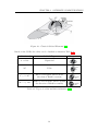
Based on the COEs, the orbits can be classified as shown in Table 2.1.
Inclination (i)
Orbital Type
0○ or 180○
Equatorial
90○
Polar
0○ ≤ i < 90○
Direct or Prograde (moves in the
direction of Earth’s rotation)
90○ < i ≤ 180○
Indirect or Retrograde (moves against
the direction of Earth’s rotation)
Diagram
Table 2.1: Types of orbits and their inclination [12]
12
CHAPTER 2. SATELLITE COMMUNICATIONS
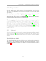
Although it is not part of the COEs, orbits can also be sorted by their altitude.
NASA’s classification divides orbits in three groups (Table 2.2).
Orbit
Altitude (a)
Low Earth Orbit (LEO)
Medium Earth Orbit (MEO)
High Earth Orbit (HEO) or
Geosynchronous (GSO)
Uses
Scientific and weather
a < 2000Km
satellites
2000Km ≤ a < 36000Km
GPS
Communications
36000Km
(phones, television,
radio)
Table 2.2: NASA’s classification of orbits [13]
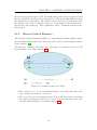
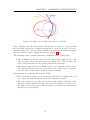
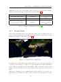
2.1.3
Ground Tracks
The satellite ground tracks are the projection of its orbit onto Earth, they are
used to clearly explain how the satellites move in reference to an observer on the
ground. An example of this can be Figure 2.4.
Figure 2.4: Ground Tracks of ESTCube-1
In an ideal two-body solution and if Earth did not rotate, the representation of
a satellite’s orbit would be a single line, as the ground track would continuously
repeat. However, Earth rotates at 1600 km/hr. Thus, even if the orbit does not
change, from the Earth-based observer’s point of view it appears to shift to the
west.
This poses a challenge to the communication with the satellite. It is visible, as a
fast moving object in the sky, from a certain location on the ground for very short
13
CHAPTER 2. SATELLITE COMMUNICATIONS
periods of time. Thus, the communications antenna needs to track the satellite
in order to handle the communication. The tracking is based on two-line element
sets, which will be covered in the next section.
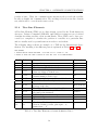
2.1.4
Two-Line Elements
A Two-Line Element (TLE) set is a data format created by the North American
Aerospace Defense Command (NORAD) and NASA to transport sets of orbital
elements describing satellite orbits around Earth. These TLEs can be later processed by a computer to calculate the position of a satellite at a particular time
and are usually used by ground stations in order to track them.
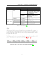
The following snippet shows an example of a TLE for the International Space
Station. The meaning of its different parts is explained in Tables 2.3 and 2.4.
ISS (ZARYA)
1 25544U 98067A 13166.62319444 .00005748 00000-0 10556-3 0 120
2 25544 51.6483 116.0964 0010829 73.3727 265.7013 15.50799671834453
Field
1
2
3
Columns
01
03-07
08
4
10-11
5
12-14
6
7
15-17
19-20
8
21-32
9
34-43
10
45-52
11
12
13
54-61
63
65-68
14
69
Content
Line number
Satellite number
Classification (U=Unclassified)
International Designator
(Last two digits of launch year)
International Designator
(Launch number of the year)
International Designator (Piece of the launch)
Epoch Year (Last two digits of year)
Epoch (Day of the year and fractional
portion of the day)
First Time Derivative of the Mean Motion
Second Time Derivative of Mean Motion
(decimal point assumed)
BSTAR drag term (decimal point assumed)
Ephemeris type
Element number
Checksum (Modulo 10)
(Letters, blanks, periods, plus signs = 0;
minus signs = 1)
Table 2.3: Two-Line Element set format definition, Line 1
14
Example
1
25544
U
98
067
A
08
264.51782528
-0.00002182
00000-0
-11606-4
0
292
7
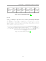
CHAPTER 2. SATELLITE COMMUNICATIONS
Field
1
2
3
Columns
01
03-07
09-16
4
18-25
5
27-33
6
7
8
9
10
35-42
44-51
53-63
64-68
69
Content
Line number
Satellite number
Inclination [Degrees]
Right Ascension of the Ascending
Node [Degrees]
Eccentricity (decimal point assumed)
(Launch number of the year)
Argument of Perigee [Degrees]
Mean Anomaly [Degrees]
Mean Motion [Revs per day]
Revolution number at epoch [Revs]
Checksum (Modulo 10)
Example
1
25544
51.6416
247.4627
0006703
130.5360
325.0288
15.72125391
56353
00000-0
Table 2.4: Two-Line Element set format definition, Line 2
2.2
Data
The data exchanged between a satellite and the ground stations on Earth can be
divided into three different categories: the beacon, the telemetry and the telecommands.
2.2.1
Beacon
A beacon is a radio signal transmitted continuously or periodically over a specified
radio frequency. It provides a small amount of information such as identification
or location, but it can have more applications. Examples of these are: adjust the
power of the ground station signal based on the beacon’s strength or tune the
ground station to compensate the Doppler shift.
2.2.2
Telemetry
Telemetry is the data generated by the payloads and the different sensors of the
satellite which is then sent to the ground station. It can be divided into two subcategories.
The housekeeping data provides information about the health and operating status
of the satellite. Examples of this data can be pressure, voltages and currents, or
also bits representing the operational status of all the components as it is shown in
Figure 2.5. The size of this data is usually quite small, so a bit rate of only a few
hundreds of bits per second is enough to complete the transmission successfully.
15
CHAPTER 2. SATELLITE COMMUNICATIONS
Figure 2.5: Telemetry user interface of the ground station software of the satellite
MaSat-1
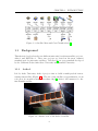
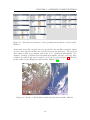
As its name states the payload data is generated by the satellites payloads, which
are the reason why the satellite has been developed in the first place. The payload
data changes with every mission and needs to be considered individually. For
example, scientific or Earth-observing missions normally generate very large data
volumes, specially in the form of images, as it can be seen in Figure 2.6, the first
picture taken by the Hungarian nanosatellite MaSat-1 [16].
Figure 2.6: Picture of South Africa taken from the nanosatellite MaSat-1
16
CHAPTER 2. SATELLITE COMMUNICATIONS
2.2.3
Telecommands
The telecommands are sent from the ground station to the satellite. They are used
to remotely control its functions and are divided into three basic types [11]:
• Low-level on-off commands. These are logic-level pulses used to set or reset
log flip-flops.
• High-level on-off commands. Higher-powered pulses, capable of operating a
latching relay or RF waveguide switch directly.
• Proportional commands. Digital words. Used for purposes such as reprogramming memory locations on the on-board computer or setting up registers in the attitude control subsystem.
2.3
Ground Station
One integral part of every satellite mission is the ground station (Figure 2.7). It
works as the first and final piece of the communication link. Its main functions
are the following:
• Tracking the satellite to determine its position in orbit.
• Gather data to keep track of the satellite’s data and status.
• Command operations to control the different functions of the satellite.
• Process the received engineering and scientific data to present it in the required formats.
17
CHAPTER 2. SATELLITE COMMUNICATIONS
Figure 2.7: Diagram of a ground station
It is important to remember that university satellites are usually classified as
amateur satellites. This means that they use amateur radio frequencies and the
usage of the ground station is bound to each country’s amateur radio regulations.
18
CHAPTER 2. SATELLITE COMMUNICATIONS
2.3.1
Ground station hardware
The main components of a ground station are the antenna, the transceiver, the
data recorders and the computers and their peripherals.
Antennas
The main hardware component of a ground station is the antenna. Its functions
may include tracking, receiving telemetry, sending telecommands, etc.
The frequencies most commonly used for amateur satellites are shown in Table
2.5.
Name
VHF
UHF
S-Band
X-Band
Frequency Range
30 to 300 Mhz
0.3 to 3 Ghz
2 to 4 Ghz
8 to 12 Ghz
Wavelength
10 to 1 m
1 to 0.1 m
15 to 7.5 cm
37.5 to 25 mm
Table 2.5: Common radio frequencies used for amateur satellite communications
Transceiver
A transceiver is a hardware unit containing both a transmitter and a receiver. It
acts as an intermediary between the antenna and a computer, changing the radio
frequency into bytes and viceversa.
2.3.2
Software
The activity in the ground station does not start when the satellite is passing over
it and does not end once the satellite is gone. There are certain tasks that need
to be done before, during and after the pass.
Before the satellite arrives it is necessary to determine and predict its orbit. Based
on this prediction the software will schedule future passes and generate the command list which will be sent during the pass.
The real-time software comes into operation when the satellite is visible from the
ground station. It is in charge of controlling the antenna rotor to follow it across
the sky; it will also send telecommands to the satellite and verify their correct reception. In addition, it will receive the data being transmitted from the satellite,
19
CHAPTER 2. SATELLITE COMMUNICATIONS
which will be processed later.
Once the satellite is not visible any more the post-pass software comes into play.
The data received during the pass is now processed and stored so the specialists
can analyse it.
Currently, there are many different kinds of software being used by amateur satellite missions. Examples of this are GPredict [17] and Orbitron [18], which are
used for tracking and prediction, or Carpcomm [19], which amongst other functionalities aims to build a network of ground stations.
There is also professional software aiming to build ground station networks. One
example is GENSO, a project of the European Space Agency (ESA) coordinated
by its Education Office. The University of Vigo in Spain hosts the European
Operations Node and coordinates the access to the network [20]. At the same
time, and as a cooperation with the ESTCube-1 project, CGI Group Inc. is
supervising the development of similar solution, Hummingbird [21], which will
be explained more deeply in the following chapters, as this thesis is part of the
mentioned project.
2.3.3
Protocols
A protocol is an agreement between the communicating parties on how communication is to proceed [22]. This section will be focused on the OSI Reference model
as well as on some of the most popular protocols for amateur satellite communications.
The OSI Reference Model
The Open Systems Interconnection (OSI) Reference Model was developed in 1983
and revised in 1995. This model deals with connecting systems that are open for
communication with other systems. It consists of seven layers which are explained
in Table 2.6.
20
CHAPTER 2. SATELLITE COMMUNICATIONS
Data Unit
Host Layers
Data
Segments
Media Layers
Packet/Datagram
Frame
Bit
OSI Model
Layer
7. Application
Function
Network process to application.
Data representation, encryption
and decryption, convert machine
6. Presentation
dependent data to machine
independent data
Interhost communication,
managing sessions between
5. Session
applications
End-to-end connection,
4. Transport
reliability and flow control
Path determination and
3. Network
logical adressing
2. Data link
Physical addressing
Media, signal and
1.Physical
binary transmission
Table 2.6: OSI Model [22]
AX.25
AX.25 is a data link layer protocol designed for use by amateur radio operators. It
occupies the first, second and third layers of the OSI model. However, AX.25 was
developed before the model came into action, so its specification was not written
to separate into OSI layers.
The link-layer packet radio transmission takes place in small blocks of data called
frames. Those frames are represented in the Figures 2.8 and 2.9.
Figure 2.8: AX.25 Supervisory and Unnumbered frames [23]
21
CHAPTER 2. SATELLITE COMMUNICATIONS
Figure 2.9: AX.25 Information frame [23]
FX.25
FX.25 is an extension to the AX.25 protocol. It has been created to complement
the AX.25 protocol, providing an encapsulation mechanism that does not alter
the AX.25 data or functionalities. AX.25 packets are easily damaged, and this
extension intends to remedy the situation by providing a Forward Error Correction
(FEC) capability at the bottom of Layer 2.
Figure 2.10: FX.25 frame structure [24]
22
Chapter 3
Hummingbird: the open source
platform for monitoring and
controlling remote assets
The continuous growth of the popularity of small satellites has been accompanied
by an increased interest in creating better solutions for controlling the satellites
from Earth. The missions are growing more complex and the use of software oriented for amateurs is starting to prove insufficient. For this reason, nowadays,
there are several projects to build professional-like software and ground station
networks to control small satellites. This chapter introduces one of them, Hummingbird [25] the project into which the work carried out in this thesis will be
integrated.
3.1
Overview
Hummingbird is an open source project aiming to create a professional like infrastructure for monitoring and controlling remote assets. It is meant to be highly
adaptable, easy scalable and be a baseline so anyone can easily build their own
solutions based on this.
It is mainly written in Java [26] and takes advantage to modern software development tools such as Apache Camel [27] and ActiveMQ [28].
23
CHAPTER 3. HUMMINGBIRD: THE OPEN SOURCE PLATFORM FOR
MONITORING AND CONTROLLING REMOTE ASSETS
3.2
Functionalities
The different modules of the system provide the following functionalities: [29]
• Telemetry limit checking and calibration.
• Telecommands configuration, validation and scheduling.
• Orbit propagation.
• Contact prediction.
• Ground station monitoring.
• Packet coding.
• Data handling.
• Scripting (including most common languages, such as Python and Javascript).
• Storage and distribution using the most common protocols.
3.3
Architecture
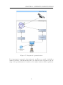
Hummingbird is a distributed, component based service-oriented system. It is
divided in three tiers: transport, business and presentation.
The transport tier is based on Apache Camel and ActiveMQ. It transports messages between different components and is a black box from the business and
presentation tiers point of view.
The business tier contains the business logic of the system. Command creation,
limit checking, calibration, scheduling and all other business operations are performed here. This tier does not care about the protocols used to broker the messages, it sends and receives them from a message bus, the transport tier.
The presentation tier is where the data is displayed. There are a number of GUIs
available, such as web GUIs, OpenGL based GUIs and OSGI GUIs. Apache Camel
is not used for their implementation and they are very independent from the Hummingbird infrastructure.
24
Chapter 4
Requirements
This chapter covers the software requirements for the two modules this thesis is
composed of. They are based on the recommendations provided by the scientists
working on the ESTCube-1 project. The chapter is organised in three sections,
the first one being the requirements which are common to both modules whereas
the following two go through each module’s requirements more in depth.
4.1
4.1.1
Common information for both modules
General Description
Product Perspective
The modules are part the Hummingbird project based on the advise and needs
dictated by the ESTCube-1 team members. For more information about Hummingbird see Chapter 3 and for more information about ESTCube-1 see Chapter
1.
General Constraints
• The modules must be licenced under Apache License v2.0 [31].
• The use of open source tools is recommended.
• The main programming language must be Java [26].
25
CHAPTER 4. REQUIREMENTS
4.1.2
External Interface Requirements
Software Interfaces
Parameter
The modules will receive Parameters. The Parameter type is part of Hummingbird
and is represented as follows:
• Numeric value (can be any type).
• Unit of the value.
• Description: additional information about the parameter.
• Timestamp: date and time when the parameter was created.
Apache Camel [27]
Since Hummingbird uses Apache Camel for the communication between modules,
the parameters for calibration are received and sent back using this system. In
addition, Hummingbird has a heartbeat service to check if the module is responding
properly. It is necessary to configure the module so it sends and receives messages
through Apache Camel.
Communications Interfaces
JMS [30]
The communication interface with the other components in the system is the
Java Message Service using Apache Camel. The module is a JMS client in a
publish/subscribe model.
4.1.3
Non-Functional Requirements
Reliability
The software should handle unexpected values correctly. Eg. the value of the
parameter is null or NaN.
Availability
Hummingbird setup can work without the modules. However, they must run for
days without problems.
Security
Handled by Hummingbird.
Maintainability
XML configuration at startup.
26
CHAPTER 4. REQUIREMENTS
Portability
Since it is written in Java it should work wherever a JVM is available.
4.2
4.2.1
Calibration module
Introduction
Scope
This software is intended to serve as an independent calibration module for Hummingbird. As such, it will receive parameters with raw values, calibrate those
values and generate new parameters which will be available for other modules in
the system to use. The system must be flexible and allow users to define their own
calibration scripts.
Definitions
• Engineering values: result of the calibration process.
• Raw values: values received from the satellite, before going through the
calibration process.
• Hummingbird: see Chapter 3.
4.2.2
General Description
Product Perspective
Common to both modules. Please see the section 4.1.1.
Product Functions
• Information input
– Allow the user to input the calibration information as an XML file.
– Parse the XML configuration to generate the calibration scripts.
• Calibration process
– Receive one raw parameter and return one calibrated parameter.
– Receive one raw parameter and return several calibrated parameters.
27
CHAPTER 4. REQUIREMENTS
– Receive several raw parameters and return one calibrated parameter.
– Receive several raw parameters and return several calibrated parameters.
User Characteristics
• Specialists/Scientists
– Frequency of use: at the moment of inserting the calibration information.
– Functions used: XML file to insert the calibration information. Other
than that, the process is automated.
– Technical expertise: Comfortable with XML and shell scripting. Also
with simple Java programming.
General Constraints
Common to both modules. Please, see section 4.1.1.
User Documentation
• Manual for specialist/scientists who will be writing the calibration scripts.
The manual must contain examples of the XML format and the way of
representing the calibration scripts.
4.2.3
External Interface Requirements
Software Interfaces
In addition to receiving Parameters this module also generates and sends them.
For more information see the section 4.1.2 as the interface is common for both
modules.
Communications Interfaces
Common to both modules. Please, see section 4.1.2.
28
CHAPTER 4. REQUIREMENTS
4.2.4
Functional Requirements
Read configuration
Introduction
The first thing the software should do is parsing the configuration files to generate
the calibration information.
Inputs
XML files with calibration information for the different subsystems.
Processing
1. Find XML files in the selected location.
2. Find calibration information available in each file.
3. Generate calibration table.
Outputs
The process will generate a table with the calibration information for all the different parameters.
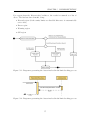
Listen to incoming parameters
Introduction
The module will be waiting for new parameters to arrive. When a parameter
is ready for calibration it will be sent to the calibrator.
Inputs
Parameters received through Apache Camel.
Processing
1. Receive a parameter.
2. If the parameter is ready for calibration send it to the calibrator.
3. If the parameter needs more parameters to be calibrated wait for those parameters.
29
CHAPTER 4. REQUIREMENTS
Outputs
The output will be one or several parameters which will be sent back to the message queue using Apache Camel.
Error Handling
• If no calibrator is found for the parameter log the error and ignore it. No
data return to Apache Camel is expected.
• If there is a problem with the calibrator log the error and do not return any
data through Apache Camel.
Calibrate
Introduction
When a parameter is ready for calibration it must be sent to the calibrator, including any extra parameters needed for the calibration and also the calibration
information.
Inputs
Parameter to be calibrated plus all extra parameters needed to do so.
Processing
1. Receive parameter(s) needed for calibration.
2. Receive all the calibration information.
3. Use the script to generate the new value.
4. Return the new parameter.
Outputs
The output will be one or several parameters.
Error Handling
If there is an error it must be sent upwards.
30
CHAPTER 4. REQUIREMENTS
4.2.5
Non-Functional Requirements
Common to both modules. Please see section 4.1.3.
4.3
4.3.1
Limit checking module
Introduction
Scope
This software is intended to serve as an independent limit checking module for
Hummingbird. It will receive a parameter and return information about the state
of that parameter in relation to the limits.
Definitions
• Hummingbird: see Chapter 3.
• Parameter: contains the value.
• State: a boolean value reporting the state of the parameter.
4.3.2
General Description
Product Perspective
Common to both modules, please see the section 4.1.1.
Product Functions
• Information input
– Allow the user to input the limit checking information as an XML file.
– Parse the XML configuration to generate the limits.
User Characteristics
• Specialists/Scientists
– Frequency of use: at the moment of inserting the limit checking information.
31
CHAPTER 4. REQUIREMENTS
– Functions used: XML file to insert the limit checking information.
Other than that, the process is automated.
– Technical expertise: Comfortable with XML.
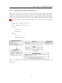
General Constraints
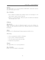
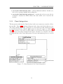
In addition to the constraints common to both modules (see section 4.1.1) there
must be two options:
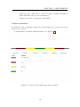
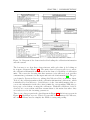
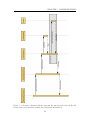
• Sanity limits, soft limits and hard limits. (See Figure 4.1).
Figure 4.1: Limit checker with sanity limits available
32
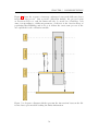
CHAPTER 4. REQUIREMENTS
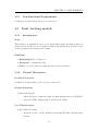
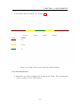
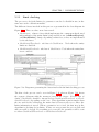
• Soft limits and hard limits only (Figure 4.2).
Figure 4.2: Limit checker only with soft and hard limits
User Documentation
• Manual for specialist/scientists who setting up the limits. The manual must
contain examples of the XML format.
33
CHAPTER 4. REQUIREMENTS
4.3.3
External Interface Requirements
Software Interfaces
In addition to the common software interfaces for both modules (see section 4.1.2)
there is one more software interface to be taken into account.
State
The module will return States. The State type is part of Hummingbird and is
represented as follows.
• value of the state (boolean).
Communications Interfaces
Common for both modules. Please see the section 4.1.2.
4.3.4
Functional Requirements
Read configuration
Introduction
The first thing the software should do is parse the configuration files to generate
the limit checking information.
Inputs
XML files with calibration information for the different subsystems.
Processing
1. Find XML files in the selected location.
2. Find limits information available in each file.
3. Generate limits table.
Outputs
The process will generate a table with the limits information for all the different
parameters.
34
CHAPTER 4. REQUIREMENTS
Listen to incoming parameters
Introduction
The module will be waiting for new parameters to arrive. Those parameters will
be sent to the limit checker.
Inputs
Parameters received through Apache Camel.
Processing
1. Receive a parameter.
2. Send parameter to limit checker.
Outputs
The output will be a list of State elements which will be sent back to the message
queue using Apache Camel.
Error Handling
• If no limit checking information is found for the parameter log the error and
ignore it. No data return to Apache Camel is expected.
• If there is a problem with the limit checker log the error and do not return
any data through Apache Camel.
Check limits
Introduction
The software must check the limits, depending on the levels of limits chosen (2 or
3) the comparison will be different.
Inputs
Parameter to be calibrated plus all extra parameters needed to do so.
35
CHAPTER 4. REQUIREMENTS
Processing
1. Receive parameter.
2. Receive the limit checking information.
3. Compare the parameter against the limits.
4. Return the result of the comparison.
Outputs
List of State elements.
Error Handling
If there is an error it must be sent upwards.
4.3.5
Non-Functional Requirements
Common for both modules. Please see section 4.1.3.
36
Chapter 5
Implementation
This chapter covers the implementation of the two software modules according to
the requirements listed in Chapter 4. To begin with, the different technologies
used to develop these pieces of software are presented. Afterwards, the design
and implementation of both modules is explained, focusing on its structure, the
relationships between the different pieces and the algorithms used to achieve the
goal.
5.1
Technologies used
As it has been explained previously, the two modules developed as part of the
work for this thesis have been designed to be integrated with the Hummingbird
project. To do so, Java [26] has been chosen as the main programming language,
as it is the language used for the development of Hummingbird. In the same way,
Apache Camel [27] and ActiveMQ [28] are used for the communication with the
rest of the modules. XStream [32] has been chosen as the library used to parse
the XML [33] files used to specify the scientific information.
The final piece of technology used is BeanShell [34], a Java-like scripting language
and interpreter which runs in the Java Runtime Environment. The calibration
module has been designed to be generic, adaptable to every mission. Also, the
goal was to make the calibration information input easy for the scientists, this
meaning that there is no need for any difficult Java programming, compilation
and so on. BeanShell integrates with the Java code and allows to run those scripts
at runtime.
37
CHAPTER 5. IMPLEMENTATION
5.2
Implementation of the calibration module
For the sake of clarity, the approach to the explanation will be in small pieces.
However, before jumping onto every small piece, it is interesting to look at the
package organization of the module.
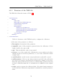
The software is divided into the following several Java packages:
• eu.estcube.calibration: contains the Apache Camel integration. It also
contains the main class of the module.
• eu.estcube.calibration.calibrate: contains the implementation of the calibrator.
• eu.estcube.calibration.constants: contains several constants used throughout the module.
• eu.estcube.calibration.domain: contains the data structures used to represent the calibration information and the calibration units.
• eu.estcube.calibration.processors: contains the main algorithm for receiving, calibrating and sending the parameters back. Also, the interface
implemented by the calibrator can be found here.
• eu.estcube.calibration.utils: contains additional utilities. In this case,
the tools to manage finding and reading files.
• eu.estcube.calibration.xmlparser: contains the tools to parse the information contained in XML format into data which can be used in the module.
5.2.1
Camel Integration
The integration with Camel is a crucial part of the module since it is where it
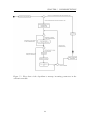
will take the parameters from. There are several classes related to this, the class
diagram of this part can be seen in Figure 5.1.
38
CHAPTER 5. IMPLEMENTATION
Figure 5.1: Class diagram of the Camel integration
Amongst the three classes represented in Figure 5.1 it is important to highlight
two of them: Calibrator and ParameterProcessor.
Calibrator is the main class of the module. As it is shown in the class diagram there
are two methods, the main method, where everything starts and the configure
method. The latter is where the integration with Camel happens, what configures
where to get the messages from, how to process them and where to send them
afterwards. In addition, Hummingbird utilizes a heartbeat system to check if the
modules are working correctly, this is also carried on here. Table 5.1 contains a
snippet of the code.
39
CHAPTER 5. IMPLEMENTATION
1
3
@Override
public void configure() throws Exception {
// @formatter:off
from(StandardEndpoints.MONITORING)
.filter(header(StandardArguments.CLASS)
.isEqualTo(Parameter.class.getSimpleName()))
.process(parameterProcessor)
.split(body())
.process(preparator)
.to(StandardEndpoints.MONITORING);
5
7
9
11
13
BusinessCard card = new ⤦
Ç BusinessCard(config.getServiceId(), ⤦
Ç config.getServiceName());
card.setPeriod(config.getHeartBeatInterval());
card.setDescription(String.format("Calibrator; version: ⤦
Ç %s", config.getServiceVersion()));
from("timer://heartbeat?fixedRate=true&period=" + ⤦
Ç config.getHeartBeatInterval())
.bean(card, "touch")
.process(preparator)
.to(StandardEndpoints.MONITORING);
// @formatter:on
15
17
19
21
23
}
Table 5.1: Camel integration Java code for the calibrator
Focusing on the part where the module receives and sends the parameters we can
see that:
• Where it gets the messages from –> from(StandardEndpoints.MONITORING)
• It only gets messages containing parameters –> .filter(header(StandardArguments.CLASS)
.isEqualTo(Parameter.class.getSimpleName()))
• What to do with the received message –> .process(parameterProcessor)
• Since the result of the processed message is a list and it is necessary to send
the parameters one by one, that result must be split. –> .split(body())
• Send it back to the messaging service
.to(StandardEndpoints.MONITORING);
40
–>
.process(preparator)
CHAPTER 5. IMPLEMENTATION
The second part - from line 14 and below - contains the heartbeat system.
ParameterProcessor contains the following:
• Part of the Camel integration.
• Code to load the calibration information from the configuration files.
• Algorithm to process the received parameters.
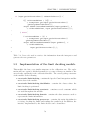
The code corresponding to the Camel integration is shown in table 5.2. The other
two parts will be explained in the following subsections.
2
4
/** @{inheritDoc . */
@Override
public void process(Exchange exchange) throws Exception {
Message in = exchange.getIn();
Message out = exchange.getOut();
out.copyFrom(in);
6
8
//The main algorithm would be placed here
10
out.setBody(calibratedParameters);
12
14
}
Table 5.2: Java code showing the Camel integration of ParameterProcessor
41
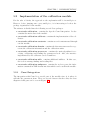
CHAPTER 5. IMPLEMENTATION
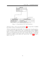
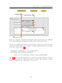
5.2.2
Loading the calibration information
The first action point when the module is initiated is loading the calibration information. This will read the information from the configuration files written by
the specialists and will create a series of calibration units which will later be used
to calibrate the incoming parameters.
Figure 5.2 shows the different classes involved in this process. They can be organised as follows:
• Main class: ParameterProcessor
• Data structures:
– CalibrationUnit
– InfoContainer
• Utils:
– InitCalibrationUnits
– InitCalibrators
– FileManager
• Parser:
– Parser
– HashMapConverter
42
CHAPTER 5. IMPLEMENTATION
Figure 5.2: Diagram of the classes involved in loading the calibration information
onto the system
The best way to see how these classes interact with each other is by looking at
its sequence diagram (Figure 5.3). The main class is ParameterProcessor, where
the calibration information will be stored in the form of a HashMap of calibration
units. The reason for choosing this data structure is its efficiency, as it provides
constant-time performance for the input and retrieval of information [35]. The process begins by ParameterProcessor asking InitCalibrationUnits to initialize them.
To do so, the calibration units need the calibration information (calibrators), which
is initialized by InitCalibrators. InitCalibrators is the class which manages the access to the information in the files; first it finds the corresponding XML files to
later parse each of them, creating the calibrators. With this calibrators, InitCalibrationUnits creates them, and then returns them to the main class where they
are ready to receive the incoming parameters.
There is one class present in the class diagram in Figure 5.2 which is not present in
Figure 5.3, HashMapConverter. This is because this class is managed by XStream,
the external library used to simplify the XML accessing and parsing.
43
CHAPTER 5. IMPLEMENTATION
Figure 5.3: Sequence diagram which represents the interactions between the different classes present when loading the calibration information
44
CHAPTER 5. IMPLEMENTATION
The data structure created to represent the calibration information is InfoContainer and it is formed by these components:
• id
– Type: String
– Content: name of the parameter to be calibrated
• outputId
– Type: String
– Content: name of the engineering parameter
• unit
– Type: String
– Content: unit in which the calibrated value is represented
• Description
– Type: String
– Content: description of the parameter
• additionalParameters
– Type: List of Strings
– Content: List with the names of any extra parameters needed for the
calibration
• resultIsVector
– Type: boolean
– Content: true if the result of the calibration is a vector, f alse if the
result of the calibration is an individual value
• scriptResultVariable
– Type: String
– Content: name of the variable which will contain the result in the script
• script
– Type: String
– Content: calibration script
This data structure is later stored within another data structure, CalibrationUnit.
The reason for using this second data structure is the way parameters are received
from Apache Camel, one by one. If all the calibrations were just simple oneparameter calibrations that would not be necessary. However, some parameters
might need information from others to be calibrated. Thus, they need to be
45
CHAPTER 5. IMPLEMENTATION
sent as a whole unit to the method which will generate the engineering values.
CalibrationUnit is formed by the following components:
• Attributes:
– id
∗ Type: String
∗ Content: name of the parameter to be calibrated
– main
∗ Type: Parameter
∗ Content: parameter which will be calibrated
– auxParameters
∗ Type: HashMap of Parameters
∗ Content: extra parameters needed to calibrate the main one
• Amongst others, CalibrationUnit can perform the following actions:
– neededParameters(): returns the parameters listed as necessary for
the calibration.
– needsThisParameter(): checks whether or not a particular parameter is needed for the current calibration unit.
– addAuxParameter(): adds an extra parameter when needed.
– isReadyForCalibration(): checks that all the needed parameters are
in place. Only when this check returns true the calibration unit is sent
to the calibrator.
– clean(): once the calibration unit has been sent to the calibrator, it is
cleaned so it can be used for the next time that parameters are received.
This means emptying the main and auxiliary parameters.
5.2.3
Calibration
The calibration process can be divided in two parts. The first one is managing the
parameters that arrive from other modules, prepare the calibration units and send
back the results. The second one is the actual calibration.
Figure 5.4 represents the class diagram of this part of the software. There are
three classes which have been seen in previous sections —ParameterProcessor,
CalibrationUnit and InfoContainer — and two new ones which are:
• ParameterCalibrator : Interface representing the method that the calibrator
must contain.
46
CHAPTER 5. IMPLEMENTATION
• Calibrate: Implementation of the previous interface, where the actual calibration is performed. This class is generic class. Its generic type T extends
from Java Number, which means any of the Java Number subtypes can be
used when instantiating it. It currently is in the form of a Double, but it can
be easily modified if ever needed.
Figure 5.4: Diagram representing the classes involved in the calibration process
Figure 5.5 is a flow chart representing the algorithm used to manage the received
parameters, in combination with the sequence diagram of Figure 5.6 they show
what the steps in the algorithm are and which parts of the software performs
then. As it was previously stated, the main class is ParameterProcessor, where
the calibration units have already been created. When a parameter is received, if
its corresponding calibration unit is available it is included as its main part (if it is
not present, the process ends and the error is logged). Afterwards, the algorithm
goes through every calibration unit doing the following:
1. Check if the parameter is needed for the calibration unit.
2. If the step 1 is true, add the parameter as an auxiliary parameter for the
calibration.
3. Check if the calibration unit is ready for calibration.
4. If the 3 is true, calibrate and save the results in a list. Finally, clean the
calibration unit.
After the whole process is completed the results are sent back to Apache Camel
to make them available for the rest of the system.
47
CHAPTER 5. IMPLEMENTATION
Figure 5.5: Flow chart of the algorithm to manage incoming parameters in the
calibration module
48
CHAPTER 5. IMPLEMENTATION
Figure 5.6: Sequence diagram describing the interactions between the different
classes when managing incoming parameters in the calibration module
The part of evaluating the raw parameters using the calibration script is left in the
hands of BeanShell. The way to evaluate a script with this library is very simple
as it can be seen in Table 5.3.
2
Interpreter interpreter = new Interpreter();
interpreter.eval(calibrationScript);
Table 5.3: Java code used to evaluate a script with BeanShell
Table 5.4 shows the way information is retrieved from the interpreter and how
the parameters with the engineering values are created. The actions to be taken
change depending on the result being a vector or not.
49
CHAPTER 5. IMPLEMENTATION
if (input.getCalibrationInfo().isResultIsVector()) {
2
T[] calibratedValues = (T[]) ⤦
Ç interpreter.get(input.getCalibrationInfo()
.getScriptResultVariable());
output.addAll(createNewParameters(input.getMain(), ⤦
Ç calibratedValues, input.getCalibrationInfo()));
4
6
} else {
8
T calibratedValue = (T) ⤦
Ç interpreter.get(input.getCalibrationInfo()
.getScriptResultVariable());
output.add(createNewParameter(input.getMain(), ⤦
Ç calibratedValue,
input.getCalibrationInfo()););
10
12
}
14
Table 5.4: Java code used to retrieve the information from the interpreter and
generate the new parameters
5.3
Implementation of the limit checking module
This module also has a very similar structure to the calibration one. The explanation will once again be divided in small pieces, some of them very similar to the
ones already explained for the calibration module. The overall package structure
of the module is the following:
• eu.estcube.limitchecking: contains the Apache Camel integration and the
main class of the module.
• eu.estcube.limitchecking.checklimits: contains the classes where the
limit checking is performed.
• eu.estcube.limitchecking.constants: contains several constants which
are used throughout the module.
• eu.estcube.limitchecking.domain: contains the data structure used to
represent the limits information.
• eu.estcube.limitchecking.processors: contains the main algorithm for
receiving, checking the limits and sending the results back. In addition, the
interface implemented by the limit checker can be found here.
50
CHAPTER 5. IMPLEMENTATION
• eu.estcube.limitchecking.utils: contains additional utilities. In this case,
the tools to manage finding and reading files.
• eu.estcube.limitchecking.xmlparser: contains the tools to parse the information contained in XML format into data which can be used in the
module.
5.3.1
Camel integration
The integration with Apache Camel is done in the exact same way as in the calibration module. Figure 5.7 contains a diagram of the classes involved in this process.
The classes change their name (Calibrator to LimitChecking and CalibratorConfig
to LimitCheckingConfig) and the split option is removed (compare to Tables 5.1
and 5.5), as there is no need to split results received from ParameterProcessor.
There are also some minor changes in the latter, but those are related to the limit
checking and not to the Camel integration. For more information please see section
5.2.1.
Figure 5.7: Class diagram of the Camel integration
51
CHAPTER 5. IMPLEMENTATION
2
@Override
public void configure() throws Exception {
4
// @formatter:off
from(StandardEndpoints.MONITORING)
.filter(header(StandardArguments.CLASS)
.isEqualTo(Parameter.class.getSimpleName()))
.process(parameterProcessor)
.process(preparator)
.to(StandardEndpoints.MONITORING);
6
8
10
12
BusinessCard card = new ⤦
Ç BusinessCard(config.getServiceId(), ⤦
Ç config.getServiceName());
card.setPeriod(config.getHeartBeatInterval());
card.setDescription(String.format("Calibrator; version: ⤦
Ç %s", config.getServiceVersion()));
from("timer://heartbeat?fixedRate=true&period=" + ⤦
Ç config.getHeartBeatInterval())
.bean(card, "touch")
.process(preparator)
.to(StandardEndpoints.MONITORING);
// @formatter:on
14
16
18
20
22
}
Table 5.5: Camel integration Java code for the limit checker
52
CHAPTER 5. IMPLEMENTATION
5.3.2
Loading the limits information
This is also done in the same way as it is performed in the calibration module.
The first action when the module is initiated is loading the limits information.
This means reading the information from the configuration files and creating the
limits which will be later used to compare against the incoming parameters. Figure
5.8 shows the different classes involved in this process. They can be organised as
follows:
• Main class: ParameterProcessor
• Data structure: InfoContainer
• Utils:
– InitLimits
– FileManager
• Parser:
– Parser
– HashMapConverter
Figure 5.8: Diagram of the classes involved in loading the limits information onto
the system
53
CHAPTER 5. IMPLEMENTATION
Figure 5.9 shows the sequence of message exchanges between the different classes
involved in this process. Just as in the calibration module, the process begins
at ParameterProcessor and the limits will also be stored in a HashMap, each
entry corresponding to a different parameter. InitLimits is the class in charge of
populating that HashMap and to do so it follows the exact same process as the
one explained for the calibration module.
Figure 5.9: Sequence diagram which represents the interactions between the different classes present when loading the limits information
54
CHAPTER 5. IMPLEMENTATION
The data structure used to represent the limits information is, as it was in the
previous module, InfoContainer. However, its inner structure differs to the one
which was previously used:
• id
– Type: String
– Content: name of the corresponding parameter.
• sanityLimits
– Type: Array of BigDecimal [36]. This number format has been chosen
as it provides high precision, avoiding rounding errors from other types,
such as double.
– Content: lower limit in the first position and and upper limit in the
second. This limits are optional, if enabled, four regions are available
(discard, error, warning and OK). Any values below the lower or above
the upper limits are discarded.
• hardLimits
– Type: Array of BigDecimal.
– Content: lower limit in the first position and upper limit in the second.
Anything between this limits and the soft limits is in the warning zone.
Anything below the lower or above the upper limits is erroneous.
• softLimits
– Type: Array of BigDecimal.
– Content: lower limit in the first position and upper limit in the second.
Anything within these limits is in the OK region.
• levels
– Type: Integer
– Content: automatically generated. Its value is 4 if sanity limits are
available,f or 3 if they are not.
55
CHAPTER 5. IMPLEMENTATION
5.3.3
Limit checking
The process to check the limits of a parameter can also be divided in two, in the
same way as the calibration module.
The different classes involved in this part are represented in the class diagram in
Figure 5.10. There are three new classes used:
• CheckLimits: abstract class which implements the common methods used
independently of the sanity limits being enabled or not. isInErrorRegion()
and checkLimits() change depending on that fact, so they are implemented
by its subclasses.
• CheckLimitsThreeLevels: subclass of CheckLimits. Used when the sanity
limits are disabled.
• CheckLimitsFourLevels: subclass of CheckLimits. Used when the sanity limits are enabled.
Figure 5.10: Diagram representing the classes involved in the limit checking process
The flow of the process can be seen in Figure 5.11 whereas Figure 5.12 shows
the sequence diagram with the messages between the classes. For the sake of
clarity, CheckLimits should be interpreted as CheckLimitsThreeLevels or CheckLimitsFourLevels, depending on the case. This algorithm is much simpler than
the one used for the calibration; the main class is ParameterProcessor, where the
limits information is stored. When a parameter is received, the first step in the
algorithm is checking for its limits. If they are not present the process will end
and error will be logged. If everything goes correctly, the parameter will be sent
to either CheckLimitsThreeLevels or CheckLimitsFourLevels.
56
CHAPTER 5. IMPLEMENTATION
Per request from the Hummingbird architect, the result is returned as a list of
State. The list has four elements, being:
• Discard region (if the sanity limits are disabled this state is automatically
set to false)
• Error region
• Warning region
• OK region
Figure 5.11: Diagram representing the classes involved in the limit checking process
Figure 5.12: Diagram representing the classes involved in the limit checking process
57
Chapter 6
User manual
6.1
Calibration module
This short user manual covers the use of the calibration module. The process is
fully automated, so the user only needs to configure the pertinent XML file containing the information related to all the parameters which need to be calibrated.
There should be one file per subsystem. This way, the person who is making the
changes will not have to be worried about modifying some other parts they do not
understand. It is advisable that each file is called as the corresponding subsystem.
The location of the folder where the XML files are stored is fully configurable by
a system property. It can be set like this: -Dpath="/path/to/the/folder".
58
CHAPTER 6. USER MANUAL
6.1.1
Structure of the XML file
The XML file follows the format of Table 6.1
1
3
5
7
9
11
13
15
<calibration>
<entry>
<id></id>
<description></description>
<outputId></outputId>
<unit></unit>
<scriptInfo>
<isVector></isVector>
<resultVariable></resultVariable>
<auxParameters></auxParameters>
<script></script>
</scriptInfo>
</entry>
</calibration>
Table 6.1: Structure of the XML file used to configure the calibrators
• id: name of the parameter to calibrate.
• Description: description of the parameter.
• outputId: name of the parameter generated after the calibration. If left
blank, it will be the same as id.
• unit: Units in which the value is represented.
• isVector: true if the result of the calibration is a vector with several values
(which generates several new parameters) or f alse if the calibration returns
a single value.
• resultVariable: variable in the script in which the result will be stored.
• auxParameters: if the are any extra parameters needed for the calibration
process it is necessary to list them here separated by commas. Please note
that if the extra parameters also need to be calibrated the parameters needed
for their calibration must also be included here in addition to the original
ones.
• script: script to generate the calibrated value. Note that if extra parameters
are needed, their calibration scripts must be included here, not the parameter
name.
59
CHAPTER 6. USER MANUAL
6.1.2
Example of simple calibration
1
3
5
7
9
11
13
15
<calibration>
<entry>
<id>parameterA</id>
<description>Example of parameter for
simple calibration</description>
<outputId>generatedA</outputId>
<unit>E</unit>
<scriptInfo>
<isVector>false</isVector>
<resultVariable>result</resultVariable>
<auxParameters></auxParameters>
<script>result = (parameterA*779.098)/35.28</script>
</scriptInfo>
</entry>
</calibration>
Table 6.2: Example of simple calibration
Table 5.7 represents the simplest example of calibration information. parameterA is the parameter to be calibrated and the user has chosen that the name
of the calibrated parameter will be generatedA. The information about the calibration script states that the result will not be a vector and the value after the
calculations will be stored in a variable called result. There are no extra parameters needed for the process to be carried on.
60
CHAPTER 6. USER MANUAL
6.1.3
2
4
6
8
10
12
14
16
Example of calibration dependent on other parameters
<calibration>
<entry>
<id>parameterA</id>
<description>Example of parameter which depends
on others to be calibrated</description>
<outputId></outputId>
<unit>E</unit>
<scriptInfo>
<isVector>false</isVector>
<resultVariable>result</resultVariable>
<auxParameters>parameterB,parameterC</auxParameters>
<script>result = (parameterA*(parameterB*2345/37))
/3145.2839 + (parameterC*2)</script>
</scriptInfo>
</entry>
</calibration>
Table 6.3: Example of calibration dependent on other parameters
Table 5.8 shows an example of a parameter which depends on others for calibration.
Again, parameterA is the name of the parameter to be calibrated. In this case
the user has not selected an output ID, so it will by default be the same as the
input. The result of the calibration will not be a vector and it needs parameterB
and parameterC to be calibrated. The calibration script can be explained as
follows:
• Calibration script for parameterA: result = ((parameterA∗(parameterB))
/3145.2839) + (parameterC)
• The user must specify parameterB’s calibration script: parameterB ∗
2345/37
• Same thing with parameterC: parameterC ∗ 2
• The final result is what can be seen in the example: result = (parameterA ∗
(parameterB ∗ 2345/37))/3145.2839 + (parameterC ∗ 2)
61
CHAPTER 6. USER MANUAL
6.1.4
Example of calibration dependent on other parameters which are dependent on others
1
3
5
7
9
11
13
15
<calibration>
<entry>
<id>parameterA</id>
<description>Example of parameter which depends
on others to be calibrated. Those other depend on ⤦
Ç others.</description>
<outputId></outputId>
<unit>E</unit>
<scriptInfo>
<isVector>false</isVector>
<resultVariable>result</resultVariable>
<auxParameters>parameterB,parameterC,parameterD</auxParameters>
<script>result = (parameterA*2)/((parameterB*4) + ⤦
Ç 5*parameterC - parameterD/4))</script>
</scriptInfo>
</entry>
</calibration>
Table 6.4: Example of calibration dependent on other parameters which also depend on others
Table 6.4, which illustrates this example can be explained as:
• Parameter to be calibrated: parameterA
• Auxiliary parameters:
– parameterA’s dependency: parameterB
– parameterB’s dependency: parameterC and parameterD
– Calibration script for parameterC: 5 ∗ parameterC
– Calibration script for parameterD: parameterD/4
– Calibration script for parameterB: ((parameterB∗4)+5∗parameterC −
parameterD/4))
– Calibration script for parameterA: (parameterA ∗ 2)/((parameterB ∗
4) + 5 ∗ parameterC − parameterD/4))
62
CHAPTER 6. USER MANUAL
6.1.5
2
4
6
8
10
12
14
Example of the result of the calibration being a vector
<calibration>
<entry>
<id>parameterA</id>
<description>Example of parameter whose calibration ⤦
Ç returns a vector</description>
<outputId></outputId>
<unit>E</unit>
<scriptInfo>
<isVector>true</isVector>
<resultVariable>result</resultVariable>
<auxParameters></auxParameters>
<script>int[] result = {parameterA*2, parameterA*3, ⤦
Ç parameterA*4};</script>
</scriptInfo>
</entry>
</calibration>
Table 6.5: Example of calibration which returns a vector as result
The module supports the interpretation of Java code and shell scripts. This example shows a short piece of Java code which will return a vector of Integer elements.
Also, it is needed to state that the result will be a vector.
6.2
Limit checking module
This subsection covers the user manual for the limit checking module. The process
is fully automated, so the user only needs to configure the pertinent XML file
containing the information related to the limits of every parameter.
There can be as many files as needed, although it is recommended to have one file
per subsystem. This way, the user will not have to be worried about modifying
some other parts they do not understand. It is advisable that each file is called as
the corresponding subsystem.
The location of the folder where the XML files are stored is fully configurable by
a system property. It can be set like this: -Dpath="/path/to/the/folder".
63
CHAPTER 6. USER MANUAL
The format of the XML file is represented in Table 6.6.
1
3
5
7
9
11
13
<limitChecking>
<entry>
<id></id>
<limits>
<sanityLower></sanityLower>
<hardLower></hardLower>
<softLower></softLower>
<softUpper></softUpper>
<hardUpper></hardUpper>
<sanityUpper></sanityUpper>
</limits>
</entry>
</limitChecking>
Table 6.6: Structure of the XML file used to configure the limits
• id: name of the parameter to calibrate which limits are to be checked.
• Sanity limits (optional): if the value is below the lower limit or above the
upper limit it is discarded.
• Hard limits:
– If the sanity limits are available anything between these limits and the
sanity limits is considered an error.
– If the sanity limits are disabled anything below the lower limit or above
the upper limit is considered an error.
• Soft limits:
– Anything between the lower and upper soft limits is considered an OK
value.
– Anything between the soft limits and the hard limits is considered OK,
but with a warning.
64
CHAPTER 6. USER MANUAL
6.2.1
2
4
6
8
10
12
Example of configuration with sanity limits
<limitChecking>
<entry>
<id>parameterA</id>
<limits>
<sanityLower>-100</sanityLower>
<hardLower>-75</hardLower>
<softLower>-20</softLower>
<softUpper>20</softUpper>
<hardUpper>75</hardUpper>
<sanityUpper>100</sanityUpper>
</limits>
</entry>
</limitChecking>
Table 6.7: Limit checking with sanity limits
6.2.2
1
3
5
7
9
11
Example of configuration without sanity limits
<limitChecking>
<entry>
<id>parameterA</id>
<limits>
<hardLower>-75</hardLower>
<softLower>-20</softLower>
<softUpper>20</softUpper>
<hardUpper>75</hardUpper>
</limits>
</entry>
</limitChecking>
Table 6.8: Limit checking without sanity limits
65
Chapter 7
Conclussions
This thesis has presented the development of a ground control software for Aalto-1
and ESTCube, satellites belonging to the increasingly popular nanosatellite family.
The ground control software chosen by these two satellite missions is Hummingbird,
an open source project aiming to create software which can be easily adaptable for
any kind of mission as well as creating a network of ground stations. It is being
developed by CGI Group Inc. in cooperation with the University of Tartu and
some external collaborators, such as the author of this thesis.
As part of this collaboration, two Hummingbird modules have been designed and
implemented. The first one being the telemetry calibration module and the second
one the limit checker.
The most challenging parts of this work have been related to the calibration module. First, an algorithm adapted to the way modules communicate in Hummingbird
had to be designed. The other challenge was finding a way to allow scientists to
input calibration information without the need of changing the Java code; the
solution chosen was to use an embedded interpreter, so anyone with knowledge of
scripting would be able to create their own calibration scripts.
The result has been two fully configurable and adaptable modules, which allow
to calibrate and check the limits of the parameters received from the satellite. If
there are changes in the mission, only the configuration files need to be updating,
making this much easier than changing the code and recompiling.
To support this process the basics of satellite to Earth communication have been
presented. Including orbits and how they affect those transmissions, the various
kinds of data transmitted, the different hardware and software components of a
ground station and the most commonly used protocols in amateur satellite communications.
66
CHAPTER 7. CONCLUSSIONS
Once the developed modules have been integrated into Hummingbird, the software
package will provide missions with an effective software which will, not only allow tracking and controlling the satellite, but generating useful scientific data and
monitoring the results automatically.
67
Chapter 8
Future work
This chapter describes the next steps to be taken towards full integration of the
two modules developed in this work with the rest of the system. The process is
described here. The future work will be carried out by the author and also by the
ESTCube-1 team.
Unit testing
Even though the software has been fully tested by the author it is intended to also
implement unit tests to cover every possible scenario. This will be done with two
different tools:
• JUnit[37]
• Mockito[38]
Test the integration with ESTCube-1’s development build
The Apache Camel code for the modules to be connected with the rest of the system has already been implemented. However, there have been no tests involving
the whole system with the two modules working. This work should be carried out
before going on any further.
Integrate with ESTCube-1’s live build and with Hummingbird
After the modules have been fully tested in the development environment and have
been approved by the people responsible of ESTCube-1’s ground segment development they should be integrated into the live build, where they will work with real
parameters received from ESTCube-1. In addition, it should also be integrated
into Hummingbird when the people in charge of the project consider it convenient.
68
Bibliography
[1] C. Singer. A Short History of Science To The Ninteeth Century p. 217.
Clarendon Press, United Kingdom, 1941.
[2] C. Robert Welti. Satellite Basics for Everyone. iUniverse, first edition. United
States, 2012. ISBN 978-1-4759-2593-7.
[3] D.J. Barnhart. Very Small Satellite Design for Space Sensor Networks. Ph.D.
thesis. Faculty of Engineering and Physical Sciences, University of Surrey.
United Kingdom, 2008.
[4] CubeSat Design Specification. Revision 12, Cal Poly. United States, 2009.
[5] J. Praks. A.Kestilä, M. Hallikainen, H. Saari, J. Antila, P. Janhunen, V. Rami.
Aalto-1 - An experimental nanosatellite for hyperspectral remote sensing. In
Geoscience and Remote Symposium (IGARS). IEEE International, 2011.
[6] A. Näsila, A. Hakkarainen, J. Praks, A. Kestilä, K. Nordling, R. Modrzewski,
H. Saari, J. Antila, R. Mannila, P. Janhunen, R. Vainio, M. Hallikainen.
Aalto-1 - A Hyperspectral Earth Observing Nanosatellite. 2011.
[7] P. Janhunen.
Electric Solar Wind Sail.
URL
electric-sailing.fi/. [Online; accessed 2013-08-05].
http://www.
[8] P. Janhunen, P.K. Toivanen, J. Polkko, S. Merikallio, P. Salminen, E. Haeggström, H. Seppänen, R. Kurppa, J. Ukkonen, S. Kiprich, G. Thornell, H.
Kratz, L. Richter, O. Krömer, R. Rosta, M. Noorma, J. Envall, S. Lätt, G.
Mengali, A.A. Quarta, H. Koivisto, O. Tarvainen, T. Kalvas, J. Kauppinen,
A. Nuottajärvi, A. Obraztsov Electric solar wind sail: Towards test missions
(Invited article). Rev. Sci. Instrum., 81, 111301, 2010.
[9]
Second Vega launch by Arianespace a success: Proba-V, VNREDSat1 and ESTCube-1 in orbit.
URL http://www.arianespace.com/
news-press-release/2013/5-7-2013-VV02-launch.asp. [Online; accessed
2013-08-07].
[10] European Space Agency. Earthnet Online - Ground Segment. URL http:
//earth.esa.int/envisat/m-s/ground/. [Online; accessed 2013-08-28].
[11] P. Fortescue, J. Startk, G. Swinerd. Spacecraft Systems Engineering. Wiley,
third edition. United Kingdom, 2003. ISBN 0-470-85102-3
69
BIBLIOGRAPHY
[12] Jerry J. Sellers Understanding Space, An Introduction to Astronautics.
McGraw-Hill, third edition. United States, 2005. ISBN 978-0-07-340775-3.
[13] NASA Catalog of Earth Satellite Orbits. URL http://earthobservatory.
nasa.gov/Features/OrbitsCatalog/. [Online; accessed 2013-04-17].
[14] T.S. Kelso Two-Line Element Set Format. CelesTrak, 2006. URL https:
//celestrak.com/columns/v04n03/. [Online; accessed 2013-04-17].
[15] B. Paige
Satellite Beacons. The Radio Amateur Satellite Corporation, 2006. URL http://www.amsat.org/amsat-new/information/faqs/
houston-net/beacons.php. [Online; accessed 2013-04-22].
[16] Masat-1 URL http://cubesat.bme.hu/en.
[17] GPredict URL http://gpredict.oz9aec.net/.
[18] Orbitron URL http://www.stoff.pl/.
[19] Carpcomm URL http://carpcomm.com/.
[20] GENSO URL http://www.genso.org/.
[21]
CGI
provides
support
for
the
launch
of
Estonia’s
first
satellite.
URL
http://www.cgi.com/en/
CGI-provides-support-launch-Estonia-first-satellite.
[Online;
accessed 2013-08-08].
[22] Andrew S. Tanenbaum. Computer Networks. Prentice Hall, fifth edition.
United States, 2010. 978-0132126953.
[23] AX.25 Link Access Protocol for Amateur Packet Radio. Tucson Amateur
Packet Radio. 1997. URL http://www.tapr.org/pdf/AX25.2.2.pdf. [Online; accessed 2013-05-03].
[24] FX.25: Forward Error Correction Extension to AX.25 Link Protocol For
Amateur Packet Radio. Stensat Group, 2006. URL http://www.stensat.
org/Docs/FX-25_01_06.pdf. [Online; accessed 2013-05-06].
[25] Hummingbird. The open platform for monitoring and control. Hummingbird,
2013. URL http://www.hbird.de. [Online; accessed 2013-06-20].
[26] Java. Oracle, 2013. URL http://www.java.com/en. [Online; accessed 201308-13].
[27] Apache Camel. The Apache Software Foundation, 2013. URL http://camel.
apache.org/. [Online; accessed 2013-05-28].
[28] ActiveMQ. The Apache Software Foundation, 2013. URL http://activemq.
apache.org/. [Online; accessed 2013-05-28].
[29] E. Eilonen, U. Kvell, L. Kimmel, G. Villemos Improving and Accelerating
Small Missions through Mission Operations Software. 5th European Cubesat
Symposium, 2013.
70
BIBLIOGRAPHY
[30]
Java Message Service. Oracle, 2013. URL http://docs.oracle.com/
javaee/6/tutorial/doc/bncdq.html. [Online; accessed 2013-08-19].
[31] Apache License 2.0. The Apache Software Foundation, 2004. URL http:
//www.apache.org/licenses/LICENSE-2.0. [Online; accessed 2013-08-19].
[32] XStream. URL http://xstream.codehaus.org/. [Online; accessed 2013-0705].
[33] Extensible Markup Language (XML). URL http://www.w3.org/XML/. [Online; accessed 2013-07-05].
[34] Pat Niemeyer. BeanShell. URL http://www.beanshell.org/. [Online; accessed 2013-07-05].
[35] Class HashMap<K,V>. Oracle, 2013. URL http://docs.oracle.com/
javase/7/docs/api/java/util/HashMap.html. [Online; accessed 2013-0705].
[36] Class BigDecimal. Oracle, 2013. URL http://docs.oracle.com/javase/
7/docs/api/java/math/BigDecimal.html. [Online; accessed 2013-07-05].
[37] JUnit. URL http://www.junit.org/. [Online; accessed 2013-08-20].
[38] Mockito. URL https://code.google.com/p/mockito/. [Online; accessed
2013-08-20].
71