1
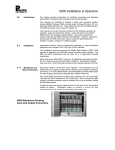
User’s Manual – Hybrid Controller
MANUAL PREPARED BY:
GILBERTO MOSQUEDA
POST-DOCTORAL RESEARCHER
STRUCTURAL ENGINEERING, MECHANICS, AND MATERIALS
DEPARTMENT OF CIVIL AND ENVIRONMENTAL ENGINEERING
UNIVERSITY OF CALIFORNIA BERKELEY
September 23, 2004
TABLE OF CONTENTS
LIST OF ILLUSTRATIONS .............................................................................................................................................. II
LIST OF TABLES .......................................................................................................................................................... III
EXECUTIVE SUMMARY ............................................................................................................................................... IV
CHAPTER 1: INTRODUCTION ........................................................................................................................................1
1.1. MISSION AND DEFINITION OF NEES@BERKELEY ................................................................................................1
1.2. OBJECTIVE .........................................................................................................................................................1
1.3. INFRASTRUCTURE OF NEES@BERKELEY ............................................................................................................2
1.4. NON-NEES INFRASTRUCTURE AVAILABLE FOR NEES@BERKELEY ...................................................................3
1.5. LOCATION AND CONTACT INFORMATION ..........................................................................................................4
1.6. MANUAL LAYOUT .............................................................................................................................................4
CHAPTER 2: BACKGROUND ..........................................................................................................................................5
2.1. HYBRID SIMULATION TEST METHOD .................................................................................................................6
2.1.1. CONTINUOUS TESTING ...............................................................................................................................7
2.2. DISTRIBUTED HARDWARE ARCHITECTURE ........................................................................................................8
2.3. EVENT-DRIVEN SIMULATION.............................................................................................................................9
CHAPTER 3: DESCRIPTION OF HARDWARE ...............................................................................................................12
3.1. HARDWARE COMPONENTS...............................................................................................................................12
3.2. HARDWARE ARCHITECTURE ............................................................................................................................13
3.3. SCRAMNET MEMORY MAP ..............................................................................................................................15
REMAINING MEMORY ........................................................................................................................................16
3.4. SCRAMENT ACCESS FROM XPC ........................................................................................................................16
CHAPTER 4: EXAMPLE APPLICATIONS ......................................................................................................................19
4.1. CONTENTS OF FOLDER UCBSTS .............................................................................................................19
4.2. PCSIMULATION MODE ..............................................................................................................................20
4.3. FAST HYBRID SIMULATION..............................................................................................................................25
4.4. SLOW CONTINUOUS HYBRID SIMULATION ......................................................................................................26
4.5. FAST-MOST....................................................................................................................................................27
CHAPTER 5: APPENDIX A: SCRAMNET MEMORY MAP .............................ERROR! BOOKMARK NOT DEFINED.
CHAPTER 6: APPENDIX B CONTROLLER SIMULATION MODES ............................................................................34
nees@berkeley: User’s Manual
Page i
LIST OF ILLUSTRATIONS
Figure 1 Test setup for hybrid simulation......................................................................................................................7
Figure 2 Ramp-hold and continuous load histories .......................................................................................................7
Figure 3 Distributed hardware architecture for geographically distributed testing........................................................9
Figure 4. Event-driven scheme using a polynomial predictor/corrector to continuously generate actuator commands
...................................................................................................................................................................10
Figure 5. Illustration of computers and networks that form the hybrid simulation testing system ..............................15
Figure 6 Simulink model template for accessing scramnet memory to MTS controller .............................................17
Figure 7. Main panel for MTS software Structural Test System (STS).......................................................................20
Figure 8. Root box diagram of Simulink model PCSimulation_hybrid.mdl ...............................................................21
Figure 9. Block ‘model’ of PCSimulation_hybrid.mdl ...............................................................................................22
nees@berkeley: User’s Manual
Page ii
LIST OF TABLES
Table 1: Training specimen specifications .................................................................. Error! Bookmark not defined.
Table 2: Test matrix of the grout test........................................................................... Error! Bookmark not defined.
Table 3: Estimation of the coefficients of friction from the grout tests ....................... Error! Bookmark not defined.
nees@berkeley: User’s Manual
Page iii
EXECUTIVE SUMMARY
This user’s manual of nees@berkeley is …
<To be written when manual is complete>
nees@berkeley: User’s Manual
Page iv
Chapter 1: INTRODUCTION
1.1. Mission and Definition of nees@berkeley
The mission of nees@berkeley is to provide a leading equipment site specializing in
earthquake response simulation of large-scale structural and non-structural systems through realtime integration of computer models and physical test specimens in a reaction wall facility.
The nees@berkeley facility is an integral part of George E. Brown, Jr. Network for
Earthquake Engineering Simulation (NEES) established by the US National Science Foundation.
The role of nees@berkeley is to ensure the availability of the state-of-the-art technology in largescale earthquake hybrid simulations involving computer modeling and physical testing and
innovative application to the field of earthquake engineering.
The nees@berkeley equipment site supports large-scale simulation by:
•
Leading the development of the hybrid simulation methods to enable:
o High-speed testing
o Advanced and robust computational tools
o Hybrid substructures (i.e. computational and physical substructures)
o Geographically distributed hybrid simulation
•
Implementing data/metadata capabilities of NEES grid
•
Simulating tests in a virtual mode prior to physical testing
•
Allowing versatile capabilities for specimen and setup configurations
•
Integrating a NEES Equipment Site to the number one rated Civil Engineering
education program
The accessibility of nees@berkeley and its proximity to several major research
universities, national research laboratories, and leading earthquake engineering professional
community provide an excellent environment for efficient collaboration with other researchers.
Moreover, nees@berkeley provides excellent ancillary research infrastructure, including office
space, computational facilities, and the 100,000 volume Earthquake Engineering Library.
1.2. Objective
This user’s manual is aimed to familiarize the interested user with the hybrid simulation
controller provided by nees@berkeley. It is assumed that an external user of the nees@berkeley
facility will only program hybrid simulation algorithms using the Matlab/xPC environment and
operating their program during the test. Thus, this manual focuses on using Simulink and xPC
nees@berkeley: User’s Manual
Page 1
along with the MTS controller and Pacific Data Acquisition for the implementation of hybrid
simulation algorithms. It is expected that experienced on-site personnel will operate the main
servo-controller or Structural Testing System (STS) controlling the actuators. Documentation on
the use of the STS software package is available for interested users (MTS 2003). Separate
documentation on use of the Pacific Instruments data acquisition software is also available. The
user should refer to related users manual for setting up test specimen in the strong floor,
calibrating instrumentation and tuning actuators.
1.3. Infrastructure of nees@berkeley
1. The nees@berkeley laboratory consists of the following:
2. A 6 m × 18 m (20 ft × 60 ft) structural tie-down floor with 60 mm (2.5 in.) tie-down
holes located in an array at 910 mm (36 in.) on center to accommodate service load of
445 kN (100 kip) acting either up or down for each tie-down hole
3. A 17.8 MN (4,000 kip) capacity Southwark-Emery Universal Testing Machine
4. An overhead 107 kN (12 US-ton) capacity bridge crane
5. A 15.2 m × 30.5 m (50 ft × 100 ft) paved construction area
6. Twenty four 3050 mm × 2740 mm × 760 mm (120 in. × 108 in. × 30 in.) hollow
modular reinforced concrete wall units that may be post-tensioned to the floor using
12 threaded rods with a prestressing force of 445 kN (100 kip) per rod to build one or
more reaction walls up to 13 m (42.5 ft) in height with the maximum shear force and
bending moment of 1780 kN (400 kip) and 5420 m-kN (4000 ft-kip), respectively
7. Two dynamic actuators with force capacity ±667 kN (±150 kip) static, ±556 kN
(±125 kip)@510 mm/s (20 in./s); stroke capacity 510 mm (20 in.)
8. Two dynamic actuators with force capacity ±979 kN (±220 kip) static, ±623 kN
(±140 kip)@510 mm/s (20 in./s); stroke capacity 1020 mm (40 in.)
9. Three static actuators with force capacity 1460 kN (328 kip) compression, 960 kN
(216 kip) tension; stroke capacity 1830 mm (72 in.)
10. A high performance MTS digital control system capable of operating up to 8 dynamic
actuators simultaneously
11. A fiber-optic network linking the MTS controller and a number of local personal
computers enabling high-speed hybrid simulations
12. A new MTS FlexTest system and a xPC digital control system, both capable of
carrying out hybrid simulations
nees@berkeley: User’s Manual
Page 2
13. A new 128+24 channel data acquisition system
14. A wide variety of transducers
15. Capabilities for telepresence, such as high-resolution still photography, NSTC and
DV video cameras, and teleconferencing
16. A personal robot avatar for off-site users to traverse the laboratory to view progress
and talk to laboratory staff, students and others on site
17. Capabilities to computationally simulate the seismic response of test specimens and
develop computational models of substructures for hybrid simulations using the Open
System for Earthquake Engineering Simulation, http://opensees.berkeley.edu/
18. Modern video equipment for video-recording of testing and tele-presence
19. In addition to the physical facility, nees@berkeley utilizes staff with extensive
experience in earthquake engineering experimental research including previous
experience in conducting research for off-site researchers.
1.4. Non-NEES Infrastructure Available for nees@berkeley
20. In addition to the nees@berkeley equipment mentioned above, the following
equipment can also be made available to researchers using nees@berkeley:
21. Two 300 kHz, 15 bit A/D converters with 144 channels of signal conditioning
22. Three 100 kHz, 12 bit A/D converters with 48 channels of signal conditioning
23. Five sets of 16 channels each, 12 bit resolution, ISA BUS data acquisition cards
without signal conditioning
24. 424 channels, 16 bit resolution, GPIB BUS with signal conditioning
25. A total of 35 static actuators with the following specifications:
26. Two actuators with 6672 kN / 610 mm (1500 kip / 24 in.)
27. Two actuators with 4190 kN / 250 mm (942 kip / 10 in.)
28. Two actuators with 2046 kN / 510 mm (460 kip / 20 in.)
29. Two actuators with 2046 kN / 250 mm (460 kip / 10 in.)
30. One actuator with 1334 kN / 300 mm (300 kip / 12 in.)
31. Four actuators with 667 kN / 910 mm (150 kip / 36 in.)
32. Four actuators with 556 kN / 910 mm (125 kip / 36 in.)
33. Two actuators with 556 kN / 610 mm (125 kip / 24 in.)
34. One actuator with 543 kN / 510 mm (122 kip / 20 in.)
35. One actuator with 351 kN / 300 mm (79 kip / 12 in.)
nees@berkeley: User’s Manual
Page 3
36. One actuator with 338 kN / 300 mm (76 kip / 12 in.)
37. Two actuators with 285 kN / 300 mm (64 kip / 12 in.)
38. One actuator with 222 kN / 300 mm (50 kip / 12 in.)
39. Two actuators with 156 kN / 2540 mm (35 kip / 100 in.)
40. Four actuators with 129 kN / 100 mm (29 kip / 4 in.)
41. Two actuators with 89 kN / 300 mm (20 kip / 12 in.)
42. Two actuators with 53 kN / 300 mm (12 kip / 12 in.)
43. Reciprocating dynamic shaker capable of developing 22 kN (5 kip) of inertia force up
to 10 Hz
<Check the above list and see if there is opposition to include the non-nees equipment>
1.5. Location and Contact Information
Nees@berkeley is located in Building 484 at the Richmond Field Station of the
University of California, Berkeley.
Address:
Richmond Field Station, Building 484
Mailing address: 1301 S. 46th Street, RFS 451, Richmond, CA 94804
Phone:
+510 231-9527
Fax:
+510 231-9471
Web site:
http://nees.berkeley.edu/
1.6. Manual Layout
A short background describing the hardware architecture for hybrid testing, including
capabilities for geographically distributed substructures are provided in the background section
in Chapter 2. Chapter 3 describes the individual hardware components that compose the hybrid
controller and their role during a simulation. After presenting the equipment, Chapter 4 presents
several example applications in detail, highlighting the steps involved in conducting a hybrid
simulation.
nees@berkeley: User’s Manual
Page 4
Chapter 2: BACKGROUND
Hybrid simulation is a method intended to evaluate the seismic performance of structures.
The principles of the hybrid simulation test method are rooted in the pseudodynamic testing
method developed over the past 30 years (Takanashi et al. [1], Takanashi and Nakashima [2],
Mahin et al. [3], Shing et al. [4], Magonette and Negro [5]). In a hybrid simulation, the dynamic
equation of motion is applied to a hybrid model, which includes both numerical and
experimental substructures. Typically, the experimental substructures are portions of the
structure that are difficult to model numerically, thus, their response is measured in a laboratory.
Numerical substructures represent structural components with predictable behavior: they are
modeled using a computer.
Hybrid simulation procedures have advanced considerably since the method was first
developed. Early tests utilized a ramp-hold loading procedure on the experimental elements.
Recently developed techniques along with advancements in computers and testing hardware
have improved this test method through continuous tests at slow (Magonette [6]) and fast rates
(Nakashima [7]). The potential of the hybrid simulation test method has been further extended by
proposing to geographically distribute experimental substructures within a network of
laboratories, then link them through numerical simulations using the internet (Campbell and
Stojadinovic [8]). The infrastructure of the George E. Brown Jr. Network for Earthquake
Engineering Simulation (NEES) provides the experimental equipment, the analytical modeling
tools and the network interface to research complex analytical models with the simultaneous
testing of multiple large-scale experimental substructures using the distributed hybrid simulation
approach. Geographically distributed hybrid simulation has already been carried out jointly
between Japan and Korea (Watanabe et al. [9]), in Taiwan (Tsai et al. [10]) and in the U.S. as
part of the NEES efforts (MOST [11]). However, these applications of distributed hybrid
simulation have used the ramp-hold procedure to load the experimental substructures. As such,
they are not benefiting from the advanced continuous methods that can improve the measured
behavior of the experimental substructures and the reliability of the test results.
The difficulty in applying real-time based continuous algorithms to distributed
applications stems from their lack of suitability with tasks that involve random completion times.
Random completion times in network communication, numerical integration and other such tasks
could compromise the stability of real-time algorithms because they may not complete in the
time required by the real-time test clock. The ramp-hold loading procedure can be readily
nees@berkeley: User’s Manual
Page 5
applied to deal with random delays since the hold period can be arbitrarily long. However, the
ramp-hold procedure introduces a number of other errors. In order to maintain the benefits of
continuous testing, an event-driven procedure is proposed for conducting continuous tests over a
network that minimizes, if not eliminates, the hold phase at each integration step. The distributed
hardware architecture utilizing event-driven controllers is also presented.
2.1. Hybrid Simulation Test Method
The equipment used for quasi-static testing in most structural testing facilities can also be
utilized to conduct hybrid tests. The basic components of a pseudodynamic test setup and their
interconnections are illustrated in block diagram form in Figure 1. The required tools are: (1) a
servo-hydraulic system consisting of a controller, servo-valve, actuator and pressurized hydraulic
oil supply; (2) a test specimen with the actuators attached at the point where the displacement
degrees of freedom are to be imposed; (3) instrumentation to measure the response of the test
specimen; and (4) an on-line computer capable of computing a command signal based on
feedback from the transducers.
The primary task of the on-line computer is to integrate the equation of motion utilizing
the restoring force vector, ri, which is composed of forces from experimental and numerical
substructures. A time-stepping integration procedure is used to solve the discretized equation of
motion for displacement, d, velocity, v, and acceleration, a, at time intervals ti =i∆t for i=1 to N.
Mai + Cvi + ri = f i
The subscript i denotes the time-dependant variables at time ti, ∆t is the integration time step and
N is the number of integration steps. The mass matrix, M, damping matrix, C, and applied
loading, f, are typically modeled as part of the numerical simulation. Numerical methods used to
solve the equation of motion are discussed in Mahin and Shing [12]. The same methods are
extended to hybrid simulation.
nees@berkeley: User’s Manual
Page 6
hydraulic supply
dc
integrator
signal generation
D/A
PID
servo-valve
actuator
da = actual imposed displacement
dc = command displacement
dm = measured displacement
rm = measured restoring force
Controller
on-line computer
servo-hydraulic system
dm
rm
A/D
da
specimen
transducers
A/D
experimental substructure
Figure 1 Test setup for hybrid simulation
2.1.1. Continuous Testing
Applying a continuous load history, rather than a ramp-hold load history, improves the
measured behavior of the experimental substructure (Magonette [6]). The improvements are
largely based on the elimination of the hold phase and the associated force relaxation in the
experimental specimens. Continuous testing methods require a real-time platform to ensure the
commands for the servo-hydraulic controller are updated at deterministic rates. Constant update
rates allow for the control of the actuator velocity, thus allowing for a continuous load history
(non-zero velocity) on the experimental elements. The difference between the ramp-hold and a
continuous load history is shown for one simulation step in Figure 2. Note that the continuous
procedure utilizing a predictor/corrector approach reduces the velocity demands for the same
time interval.
An example of a predictor/corrector technique for continuous loading is
actuator command
summarized below.
computation
di+1
corrector
predictor
di
application
ramp
computation
continuous
ramp-hold
hold
∆Ti (simulation time step)
actual time
Figure 2 Ramp-hold and continuous load histories
In their algorithm for real-time testing, Nakashima and Masaoka [13] separate the
computations in the on-line computer into two tasks running at different sampling rates: (1) the
response analysis task, which carries out the integration of the equation of motion and 2) a signal
nees@berkeley: User’s Manual
Page 7
generation task, which provides displacement commands to the servo-hydraulic actuator at a rate
faster than that of the integration time step. These two tasks run on a Digital Signal Processor
(DSP) in real-time using a multi-rate approach. The response analysis task deals with the typical
numerical algorithms for solving the equation of motion. The signal generation task, on the other
hand, computes the displacement path of the actuator using polynomial approximation
procedures. Nakashima and Masaoka showed that third order polynomial interpolation and
extrapolation of known displacement values from previous steps provide accurate displacement
and velocity predictions in the current step. The key to this polynomial approximation procedure
is that the computation time is small and actuator commands can be continuously generated at
small constant time intervals. For each integration step, the actuator is kept in motion after
achieving the target displacement by predicting a command signal based on polynomial
extrapolation of the previous target displacement values. Meanwhile, the integrator task is
carrying out computations for the next target displacement. Once the integration task has been
completed and the target displacement is known, the controller switches to interpolate towards
the correct target value. An advantageous feature of this algorithm is that the communication
between the integration task and the signal generation task is minimized.
2.2. Distributed Hardware Architecture
The typical architecture of a hybrid simulation controller consists of the integration loop
commanding the inner servo-hydraulic controller loop as previously shown in Figure 1. A single
processor is used to compute both the integration of the equation of motion and the signal
generation of the actuator commands. The separation of these two tasks into different processors
provides an expandable distributed architecture for simultaneous testing of multiple substructures
as show in Figure 3. Moreover, increased processing time can be dedicated to the integrator task
for applications with large numerical structural models. In a local testing configuration, the
network is replaced by a shared memory bus (Systrans [14]) to maintain fast communication
rates for real-time continuous algorithms. In the case of geographically distributed testing,
Ethernet replaces the network link. As will be demonstrated in the discussion of the experimental
results, network communication time is random, and therefore not suitable for real-time
algorithms. A solution based on a finite-state event-driven controller design is discussed next.
nees@berkeley: User’s Manual
Page 8
2.3. Event-Driven Simulation
In cases where task execution times are random, a clock-based control scheme could fail
if the required processes are not completed within the allotted time. As an improved alternative
to the clock-based scheme used for real-time applications, an event-driven reactive system, based
on the concept of finite state machines (Harel [15]) is proposed that responds to events based on
the state of the hybrid simulation system. The event-driven system can be programmed to
account for the complexity and randomness of real systems and, thus, take action to minimize the
random effects on experimental substructures. The programming procedure is based on defining
a number of states in which the controller can exist in and the transitions between these states
that take place as specified events occur.
Nakashima and Masaoka's [13] algorithm reacts to events in the sense that the algorithm
switches from extrapolation to interpolation after the integration task is completed. However, the
variance in task completion times for their application was minimal. They used an explicit
integration method and the DSP running these tasks had a dedicated and reliable connection to
the servo-hydraulic controller. This algorithm will not function effectively for distributed hybrid
NETWORK
simulations involving the Internet since random delays are likely to occur. The state transition
dm
DSP
Signal
Generation
dij+1
PID
Servo-hydraulic
control
rm
Actuator
Load cell
PC
Integrator Algorithm
Remote Substructure A
Analysis Site
dm
DSP
Signal
Generation
dij+1
PID
Servo-hydraulic
control
rm
Actuator
Load cell
Remote Substructure B
Figure 3 Distributed hardware architecture for geographically distributed testing
nees@berkeley: User’s Manual
Page 9
diagram in Figure 4 shows the implementation of an event-driven version of a polynomial
predictor/corrector command generation method. This algorithm continuously updates the
actuator commands using the same approach under normal operation conditions and takes action
for excessive delays. This diagram consists of five states: extrapolate, interpolate, slow, hold and
free_vibration. The default state is extrapolate, during which the controller commands are
predicted based on previously computed displacements while the integrator computes the next
target displacement. The state changes from extrapolate to interpolate after the controller
receives the next target displacement and generates the event D_update. The event D_target is
generated once the physical substructure has realized this target displacement. The model then
subsequently transitions back to the extrapolate state and sends updated measurements to the
integrator. The smooth execution of this procedure is dependent on having a reliable network
connection and selecting the run time of each integration step sufficiently large for all of the
required tasks to finish. Small variations in completion times for these tasks will only affect the
total number of extrapolation steps versus interpolation steps.
The advantage of the event-driven approach is that logic can be included to handle
excessive delays. For example, if the system is in the extrapolate state longer than a specified
time, the actuator can deviate from the intended trajectory or even exceed its target, hence limits
need to be placed on the number of allowable extrapolation steps. A simple solution is to
generate the event TimeOut, which will transition the controller to the slow state. In the slow
state, extrapolation continues at a reduced velocity to keep the actuator in continuous motion
while allowing more time to receive an update. Upon receiving the next target displacement, the
D_target
extrapolate
D_update
interpolate
free_vibration
TimeOut
D_update
D_update
TimeOut
slow
TimeOut
hold
Legend
State:
State Transition Path:
Event causing State Transition: Event/functionCall()
Figure 4. Event-driven scheme using a polynomial predictor/corrector to continuously generate
actuator commands
nees@berkeley: User’s Manual
Page 10
interpolate state is activated. If the update is not received within a set amount of time, the slow
state needs to TimeOut as well, to place the actuator on hold until the target displacement is
received. Longer delays, possibly due to the integrator crashing or a network failure, could
indefinitely delay the controller receiving an updated displacement. For this rare event, the hold
state can also time out and force the system into free_vibration or any other desirable state to
dissipate the energy in the physical specimens and end the test. The free_vibration state is
intended to fully unload the physical substructure based on locally stored mass and damping ratio
for the test specimen.
nees@berkeley: User’s Manual
Page 11
Chapter 3: DESCRIPTION OF HARDWARE
The hybrid simulation control system is composed of various computers. Each individual
computer is first described in Section 3.1 then the interconnections that form the hybrid
simulation controller are described in Section 3.2. Special attention is given to the shared
memory link in Section 3.3, particularly on how to access data from this memory for use in
hybrid simulation algorithms. Details on how to access the shared memory resource from xPC
are discussed in Section 3.4
3.1. Hardware Components
The following computer equipment forms the hybrid simulation testing system:
Simulink Host PC (Dell Precison 630 Workstation with Windows XP): is used to
program Simulink models with data signals mapped to scramnet memory. Once the Simulink
model is downloaded to the xPC, control of the model, including start, stop, and parameter
tuning, can be maintained from this computer, although the program actually runs on the xPC
Target.
xPC Target PC with scramnet (Dell Precison 630 Workstation): contains two operating
systems: (1) xPC (boot from floppy) and (2) normal Windows XP (boot from hard disk). In xPC
mode, this computer functions as a real-time processor and runs compiled Simulink models in
real-time. The programs running on the xPC are downloaded and controlled from the Simulink
Host. There is little user interaction with the xPC model. In Windows mode, this computer is
able to access scramnet, although not necessarily in real-time, and can be used to view data in
Windows applications.
Hybrid controller host PC (Dell Precison 630 Workstation with Windows XP): runs the
graphical user interface to the MTS servo-controller. The software STS can be used to calibrate
and tune instrumentation, servo-valves and actuators prior to a test. During a test, the Hydraulic
Service Manifolds (HSM) are switched on and off from this machine and the program source for
the actuator commands is selected. The controller “Program Source’ is set to ‘Scrament’ mode in
order to enable actuator commands from the xPC. Otherwise, the command signal can be
produced locally using the function generator or other available sources.
Hybrid controller hardware with scramnet (MTS Rack mount hardware) consists of MTS
VME console including digital actuator controllers, signal conditioners, and interlock
mechanisms. The controller is preset to run at a frequency of 1024 Hz, which is the update rate
nees@berkeley: User’s Manual
Page 12
for the servo-valve commands and the fastest rate at which data can be sampled. All servohydraulic components on the lab floor connect to this hardware, including servo-valves and
feedback instrumentation for control (force, displacement, deltaP). The MTS hardware includes
24 signal conditioners used primarily for feedback sensors, analog I/O, digital I/O, and encoders.
All measured data from the sensors and internal control commands are written to the scramnet
memory, also at a rate of 1024 Hz. If the controller program source is set to ‘scramnet’, the
actuator commands are obtained from a predetermined scramnet memory location.
Data acquisition host PC with GPIB (Dell Precison 630 Workstation with Windows XP)
runs the graphical user interface to manage the data acquisition hardware, including the logging
of data. Two software programs are used for this purpose, PI660 is the main software for typical
operation and Panel60 serves more as a debugging tool. The active sensor channels are defined
and calibrated through the PI660 interface. Data saved to disk using PI660 is stored in the local
hard drive.
Data acquisition hardware with scramnet, (Pacific Instruments rack mount hardware)
contains signal conditioners, a scramnet card and a DSP dedicated to data acquisition. Logged
data is collected and time-stamped by the local DSP before being sent to the host PC for writing
to disk. Sensor data is written to scramnet memory locations in units of counts. The calibration
information to convert counts to engineering units in only known by the host although the
calibration factors can be written to a separate memory location in scramnet after calibration is
completed. It should be noted that the Pacific Instruments hardware can write to the scramnet
memory but cannot read from it.
3.2. Hardware Architecture
The physical location of the hardware listed above and the interconnections between
these machines is illustrated in Figure 5. The overall setup consists of three real-time computers
with scramnet cards and three hosts that serve to interface with each of the real-time computers.
The xPC Host and Hybrid Controller Host are both connected to their real-time counterparts via
Ethernet. The data acquisition host is connected through GPIB utilizing a fiber optic cable that
provides increased throughput. The three real-time computers are connected through scramnet,
forming a closed circular loop between the three nodes as indicated in Figure 5.
Both the MTS servo-controller and the PI data acquisition system consist of specialized
hardware design to execute a particular task. However, both of these systems contain useradjustable settings and tunable parameters that can be optimized for a specific applications via
nees@berkeley: User’s Manual
Page 13
the host. The MTS servo-controller’s main task is to provide the closed loop force or
displacement control of the actuators using an enhanced PID type algorithm. Basically, the
servo-controller accepts a displacement or force command and generates the proper command
signal for the servo-valve that attempts to move the actuator to the commanded position. The PI
data acquisition hardware provides the signal conditioning and calibration capabilities to obtain
measured data from analog sensors, which can be digitized into engineering units and saved to a
file.
The only user programmable component in this system is the xPC real-time target. Of
particular importance, numerical algorithms for conducting hybrid simulations can be
programmed to run in the xPC environment in real-time. xPC has access to data from both the
MTS controller and the PI data acquisition system through scramnet. Further xPC can generate
actuator commands for the MTS controller. The scramnet memory map and access to data on
scramnet from xPC for use in numerical algorithms is discussed in more detail in the sections
that follow.
To improve the performance of the hybrid testing system, xPC and the hybrid controller
can be synchronized to insure that xPC updates the command in time for each control cycle. This
is accomplished by having the Simulink model interrupt source set to the MTS clock rather than
its own clock. The MTS models for fast hybrid testing presented later are set trigger from the
MTS clock. Due to this synchronization, the Simulink model must runs at a base rate of 1024 Hz.
nees@berkeley: User’s Manual
Page 14
Control room
xPC
Host PC
Ethernet
Hybrid Controller
Host PC
Data Acquisition
Host PC
xPC
Real-time target
GPIB
scramnet
Fiber
Ethernet
Fiber
scramnet
Fiber
MTS
Hybrid Controller
Fiber
scramnet
GPIB
Pacific Instruments
Data Aquisition
Instrumentation room
To Actuators,
HSM, pod.
To sensors.
Figure 5. Illustration of computers and networks that form the hybrid simulation testing system
3.3. Scramnet Memory Map
Scramnet provides 2MB of shared memory between computers in its network. Each
computer contains a 2MB memory module that is mirrored to all other computers on the
network. Data written to local memory on one computer is copied to the other nodes on the
network. In order to avoid conflicts between the computers using shared memory, a memory map
has been defined to coordinate the reading and writing of data from xPC, MTS, and PI.
Table 1 lists the reserved partitions in the scramnet memory. The MTS controller reads
and writes to the first memory partition of size 1024 words or 4KB. (A word is defined as 4 bytes
or 32 bits.) This includes data written by the MTS controller and data written by xPC for use by
nees@berkeley: User’s Manual
Page 15
the MTS controller. The following 1024 words of memory are reserved for the PI heartbeat
(internal clock or counter) and current sensor readings. The next 1024 words are also reserved
for PI, for the storage of calibration constants for the sensor channels. This calibration data is
only updated on scramnet when requested by the user after a calibration parameter has been
changed. The remainder of the scramnet memory is available to the user, for example, to transfer
data between other computers that may be added to the scramnet ring.
Table 1 Reserved memory partitions in shared memory resource
Partition
1-1024 words
1025-2048 words
2049-3072 words
Resource
MTS Data
PI heartbeat and real-time sensor readings
PI calibration constants
User defined
Remaining memory
The memory map for MTS, consisting of the first 1024 words, has been coded into the
controller and cannot be modified by the user. The corresponding memory map used by xPC has
been specified by MTS as a Matlab M-file (initialize.m) and should not be modified to insure
compatibility with the controller. The format in which the PI data is written to scramnet is also
pre-defined. However, the location in memory to which the PI data is written can be specified
through PI660 software. Specific details on the MTS and PI memory maps are included in
Appendix A.
3.4. Scrament access from xPC
Nees@berkeley users need to access data from xPC or other PC’s on the scramnet
network for use in their algorithms. Computers can be added to the scramnet network for
additional tasks such as OpenSEES simulations or data streaming to the NEESPOP. These
computers also need to be programmed to read from the specified locations in the shared
memory. However, only access from the xPC is discussed here.
To tools to access scramnet memory associated with the MTS controller from the xPC are
well defined. For a hybrid simulation, the Simulink model ‘FastHybrid.mdl’ provides the inputs
and outputs to the controller through scrament, which form the inputs and outputs necessary to
interact with an experimental specimen in the Simulink structural simulation. The Simulink
template FastHybrid.mdl shown in Figure 6 shows the Simulink blocks that access data from
scramnet in real-time. Figure 6a shows the complete model listing all the inputs and output and
Figure 6b shows the details of the ‘input from scrament’ block. Figure 6b demonstrates how a
nees@berkeley: User’s Manual
Page 16
continuous memory partition is input to the Simulink program then upacked into the separate
partitions. The partitions are defined in the Matlab workspace by running initialize.m to create
the memory partition structure ‘node’. Each partition is defined by specifying the variable type
and vector size for example:
% master span
baseAddress
=
partition(1).Address
partition(1).Type
=
partition(1).Size
=
% control modes
partition(2).Type
partition(2).Size
0;
= ['0x', dec2hex(baseAddress*4)];
'single';
'1';
= 'uint32';
= num2str(nAct);
The base address is defined for the first partition; the following partitions fill the memory
immediately following the previous partition. More detailed information on defining scrament
memory partitions for Simulink can be found in “scramnet.doc”, including the creation of the
‘node’ data structure after the partitions have been defined.
(a) Simulink model FastHybrid.mdl
(b) Blocks to acces input from scramnet
Figure 6 Simulink model template for accessing scramnet memory to MTS controller
The sensor readings collected by PI are also written to the scramnet memory and can be
read by the xPC Target. Use of this data requires programming for two reasons: (1) due to the
volume of data available from PI (128+16 Channels), xPC should be set to read only the
nees@berkeley: User’s Manual
Page 17
necessary channels to reduce overhead and (2) the PI data written to scramnet is in units of
counts from the A/D converters and needs to be converted to engineering units. The code below
demonstrates how to read the PI heartbeat and 128+16 data channels into partitions 25 and 26 of
the scrament memory map respectively, following 23 partitions defined for MTS.
%START PACIFIC INSTRUMENTS PARTITIONS
%blank space
partition(24).Type
partition(24).Size
= 'uint32';
= '866';
% Pacific Instruments- heartbeat (Memory Address 0X1000)
partition(25).Type
= 'int32';
partition(25).Size
= '1';
%Pacific Instruments - 128 channels + 16
partition(26).Type
= 'int16';
partition(26).Size
= '544';
First, a blank partition 24 is defined to complete the 1024 words reserved for MTS.
Starting at word 1025 (0X1000), a single partition of variable type ‘int32’ is defined for the
heartbeat followed by a partition of vector size 544 type‘int16’. PI reserves a word length (32
bits) memory slot for each channel, but since the A/D converters are 16 bit, the first 16 bits are
empty followed by the 16 bits of actual data. Further, PI reserves 8 memory locations per card;
this is the maximum number of channels per card in the system. There are 32 cards (2 Racks
with 16 cards each) with 4 channels (128 Channels) and there are two cards with 8 channels (16
channels of analog input only). Therefore, 544 ‘int16’ variables are read by xPC where every
other integer is blank data and for the 4 channel cards, the last four channels are blank. For
example to access the counts for channel ‘Pacific 65 (1:0:0)’, which is located in RACK 1,
CARD 0, CHANNEL 0, we need to skip RACK 0, which holds 16 cards. That is (16 Cards) * (8
Channels/card) * (2 integers/Channel) = 256 Integers. Therefore integers 257 and 258 are
reserved for ‘Pacific 65’, but the 16 bit integer data is stored in 258 (257 is blank). The Simulink
model Pacific_scram.mdl together with InitialzePI.m demonstrates how to read a value written
by PI from scramnet and covert to engineering units.
nees@berkeley: User’s Manual
Page 18
Chapter 4: EXAMPLE APPLICATIONS
Five examples applications of the hybrid simulation controller are presented to
demonstrate the use of the testing system. First, the contents of the directory containing the main
software is reviewed followed by the demonstrations. The first example shows the use of the
controller in PC Simulation Mode, which is a useful standalone tool for training and pre-test
simulations. PC Simulation uses a Simulink model to represent the behavior of the actuators and
specimen and a Windows based controller model, thus no hardware is necessary. The three
following examples demonstrate the use of the controller in fast hybrid mode, which is used for a
real test. There is a third option for simulation labeled real-time mode in which the controller
hardware is exercised but actuator and specimen models are used instead of the physical
actuators. The real-time mode is not described here since its use is similar to the two models
presented.
4.1. Contents of Folder ucbSTS
MTS related software is found within the ‘ucbSTS’ folder. Both the Hybrid controller
host (C:\ucbSTS) and the xPC Host (D:\MTSmodel\ucbSTS) contain copies of this folder. The
files referred to in this manual should be available in the xPC Host. Folders and files that should
be of interest to the user are listed in Table 2
Table 2. List of files in ucbSTS folder
File or Folder name
Description
Api
Matlab based api that can be used to change parameters, settings and
other STS commands. See apiExample.m.
Contains files that describe the use and setup of the hybrid controller,
including the scramnet memory map
Matlab m-files for importing MTS binary data files (*.bin) into the
Matlab workspace
Contains templates for Simulink models
Main STS control software
Setting file for STS software, contains stored gains and calibrations for a
setup. File is automatically generated by STS by saving settings.
Simulink model template for running a simulation without hardware
Simulink model template for running simulation with main controller in
the loop (runs in real-time) but models for the actuators and test setup.
Simulink model template for running a hybrid simulation with real
controller and actuator.
Contains model input parameters for above Simulink models, including
actuators, specimens, and scramnet memory map.
Documents
Matlab
Simulink
STS.exe
*.set
Simulink/PCSimulation.mdl
Simulink/RTSimulation.mdl
Simulink/FastHybrid.mdl
Simulink/Initialize.m
nees@berkeley: User’s Manual
Page 19
4.2. PCSimulation Mode
PCSimulation mode provides an option to simulate a hybrid test using a single computer
with no specialized hardware. Simulink models are provided to simulate the behavior of the
actuators and a windows-based application simulates the controller. The user needs to
incorporate specimen models and hybrid simulation algorithms into Simulink and combine with
the actuator models to run a customized simulation. Two programs are used to run PC
Simulation: STS software configures as noted below and the Simulink PCSimulation.mdl or a
modification of this model.
The STS interface to the MTS hybrid controller can operate in two modes: (1) it can
communicate with the MTS VME console that runs in real-time using TCP/IP or (2) it can
communicate with a windows model of the controller running on the same computer. The
settings file (*.set) determines the mode of operating. If there is a ‘settings.set’ file in the same
directory as STS.exe, then by default this file is used to start STS. Otherwise the user is
prompted for a settings file. Table 3 below shows the first few lines of a ‘*.set’ file, which
determines if STS runs with hardware or runs in windows simulation mode. In addition, the
‘Enable Simulation’ option must be checked in the STS main panel for simulation of the
actuators as shown in Figure 7.
Table 3. STS settings for use with hardware or PCSimulation mode
File *.set for using STS with hardware
File *.set for using STS with PCSimulation
(MySystem
podDriver 'pod.dll'
coopsDriver 'Super.dll'
userPassword ''
)
(MySystem
podDriver ''
coopsDriver 'SuperSim.dll'
userPassword ''
)
Figure 7. Main panel for MTS software Structural Test System (STS)
nees@berkeley: User’s Manual
Page 20
In addition to the MTS controller, the Simulink model PCSimulation.mdl should be
opened. Figure 8 shows a modification of this model renamed PCSimulation_hybrid.mdl, which
has been modified to conduct a hybrid simulation. The root model contains two blocks: the
‘controller’ block, which is an S-function that connects to the STS software in simulation mode
and the ‘model’ block, which contains models for the actuators and hydraulic supply. Similar to
a real setup, the controller sends valve commands to the actuator models and receives feedbacks
representing the response of the actuators. The user should become familiar with the ‘model’
subsystem, particularly the actuator and specimen models. Figure 9 shows the ‘model’ subsystem
and the implementation of a hybrid simulation algorithms using the force feedback from the
actuator models and generating the displacement commands for the servo-hydraulic controller.
Figure 8. Root box diagram of Simulink model PCSimulation_hybrid.mdl
nees@berkeley: User’s Manual
Page 21
Figure 9. Block ‘model’ of PCSimulation_hybrid.mdl.
Before presenting a simulation using the actual hybrid simulation algorithm, a simpler
model is presented to demonstrate the use of STS. In this example, the STS software is used to
excite the actuator directly without use of the hybrid simulation algorithm. The followings steps
should be followed:
1. Start \ucbSTS\STS.exe and select a *.set file
2. Start Matlab and switch to directory \ucbSTS\Simulink
3. In Matlab, run initialize.m and open Simulink model PCSimulation.mdl or
PCSimulation_hybrid.mdl (both will work)
4. Run Simulink model by clicking on the play button
5. In STS, set program source to “Function Generator” and open operation ->function
generator. Select ’Act 1 Displ’ and create a command signal, for example a sine wave.
nees@berkeley: User’s Manual
Page 22
6. Select view->oscilloscope and set CH A and CH B to ‘Act 1 disp cmd’ and ‘Act 1 displ
fbk’ then hit auto to start viewing data
7. In the main panel hit run to start the function generator. You should see the generated
displacement command in the oscilloscope. The displacement feedback should follow the
displacement command. Note that if the Simulink model is not playing, the displacement
feedback will remain constant.
8. User should try changing the controller gain (Operation->controllers) to see how the
actuators response changes to the command signal
In order to run the model using the hybrid simulation, the program source needs to be
changed to Scramnet. In this setting the controller will look for the actuator commands from the
Simulink model. In addition, the Run button must be pressed to set the span to 100%. Upon
playing PCSimulation_hybrid.mdl, the command for actuator 1 should begin to change.
Users wishing to run a PC simulation on their own computer can do so by simply copying
the USBSTS folder to their computer and running the PC simulation as indicated above. Apart
from Matlab/Simulink, no additional software or hardware is necessary.
4.3. RTSimulation Mode
RTSimulation mode provides an option to conduct a real-time simulation with xPC, xPC
Host, and MTS Host involved. From xPC Host a displacement command or a force command
can be sent through Scramnet to the MTS Host computer. A Simulink model is provided to
perform real-time reading and writing in and from Scramnet. A windows-based application
(STS) simulates the behavior of the actuators and the controller on MTS Host. The user can
check communication between the xPC, xPC Host and MTS Host. Two programs are used to run
RT Simulation: STS software configures as noted below and the Simulink RTSimulation.mdl or
a modification of this model.
On MTS Host machine:
1. run STS with setting_uNEES.set setting file. If there is a problem with running the STS
properly it is advised to reset the MTS Hybrid Controller (‘RST’ button) in the
instrumentation room.
2. set an oscilloscope to show a Scramnet command and displacement (force) feedback at
particular actuator, or Actuator 1 in this example.
3. in the main STS panel the program source should be selected as ‘Scramnet’ and
simulation mode should be enabled (Figure 10).
nees@berkeley: User’s Manual
Page 23
Figure 10. Main panel for STS in RTSimulation mode.
On xPC Host machine:
1. open RTSimulation.mdl Simulink model (Figure 11), compile it, and connect it. User can
use ‘play’ and ‘pause’ buttons in the Simulink model’s menu or enter tg.start and tg.stop
from the Matlab prompt.
2. Push ‘play’ button or type tg.start in the Matlab prompt.
3. Make sure that the flags for displacement control are assigned to zeros (they should be
equal to one for a force control mode).
4. Change value in Disp1 block (for Actuator 1) to some value, and press ‘connect’ button
in the Simulink model. The displacement value will be passed through the Scramnet to
the MTS Host, so the displacement command will take this value in the STS window of
the MTS Host computer. Once the model is playing (tg object is started) any change in
Disp1 box will result in a change in the STS oscilloscope presentation on the MTS Host
machine. If the ‘run’ button is pushed the change in the Scramnet command will cause a
change in the feedback command.
nees@berkeley: User’s Manual
Page 24
Figure 11. Simulink RTSimulation.mdl for real-time simulation.
4.4. Fast Hybrid Simulation
This example demonstrates the use of the hybrid controller to run a real-time simulation.
The integration algorithm is programmed into Simulink using an S-function and runs in realtime. In addition, a polynomial approximation procedure is incorporated to generate commands
to the actuator at 1024 HZ, regardless of the rate of the integrator. The numerical integration
algorithm can be scaled in time to run the simulation at slower rates.
The procedure to run a fast hybrid simulation is very similar to the procedure for PC
Simulation mode.
1. Once an actuator has been tuned and attached to a specimen, the STS software
controlling the real hardware should be set to ‘scramnet’ program source, HSM
nees@berkeley: User’s Manual
Page 25
turned on, and the run button pressed to set span to 100%. The controller is now
ready to accept commands from scramnet. Before hitting run, it is advisable to
check that the signal ‘Act * scram cmd’ is 0. If not, this should be set to 0 by
trying a quick tg.start, tg.stop from Matlab in the xPC Host assuming a model is
loaded.
2. On the xPC Host, open the Simulink model FastHybrid_sdf.mdl. Run
SDF_input.m to set parameters for the structural model.
3. Build and download the model to xPC. If STS is ready, type tg.start in Matlab to
start simulation. Note that the simulation starts as soon as tg.start is entered. It is
important that the actuators be ready to go at this point.
4. Data can be saved to a file using STS (limited to control signals in MTS
controller) or xPC Target.
4.5. Slow Continuous Hybrid Simulation
In the previous example, the complete simulation algorithm, including the integrator and
signal generation tasks were programmed within Simulink. Particularly for the integration
algorithm, the programming for large structural models can become difficult in Simulink. This
example demonstrates the use of multiple processors and easier programming using Matlab. The
complete structural model and the integration algorithm are programmed in Matlab, thus can be
done for complex structures. The xPC Target runs only the signal generation task, which is based
on an event-driven control strategy to deal with possible delays in the non-real-time Matlab
environment. The signal generation algorithms run in real-time using polynomial approximations
to generate actuator commands at 1024 HZ.
The necessary files to run a hybrid simulation locally using matlab and xPC can be found
in ucbSTS\Simulink\eventmdl\. The numerical model consists of a 2DOF shear building model
where the story resisting forces are obtain from two ‘experimental substructures'.
The numerical analysis in 'localsim_2dofshear.m' sends two target displacements and
receives measured response values from the Simulink model 'FastHybrid_eventmdl.mdl' running
in real-time on the xPC. The Simulink model includes a Stateflow block 'eventcommand'. (Note
that this requires 'Stateflow' and 'Stateflow Coder' to be able to compile and run in real-time.)
This block generates a continuous displacement command for the actuators at a rate of 1024Hz,
nees@berkeley: User’s Manual
Page 26
the rate of the MTS controller, using polynomial approximations. The continuous test is scaled in
time by selecting the duration of the integration step (time_step_updated in initialize_xpc.m).
The actuator target displacement commands are updated and the step number is
incremented in the xPC in each step. XPC reacts by generating the command signal for the MTS
controller and returns the measured values at the target command. Please examine the Simulink
model to verify the channels used in the MTS controller.
Steps to run the simulation:
1. In matlab, switch to the directory D:\MTSmodel\ucbSTS\Simulink\event_model
2. Run 'initialize_xpc.m'. This defines some variables for the Simulink model.
3. Build and download the Simulink model 'FastHybrid_eventmdl.mdl' to xPC
4. Start actuators (make sure disp scram cmd is set to 0)
5. Start the real-time program, for example 'tg.start'
6. Start the numerical analysis by running 'localsim_2dofshear'
You should see the real-time response computation in the host computer showing the
global displacements and the story shear vs. story drift for both stories. The xPC plots the
generated displacement command signals and the state of the controller - (0) extrapolate, (1)
interpolate, (2) slow, (3) hold. Especially if you do other things on the host PC, you should note
that the slow and hold states are activated because of delays in Matlab.
4.6. Fast-MOST
In order to run a simulation using NEESgrid software including NTCP, special software
needs to be installed and the operating system configured. To verify settings, all computers
involved both for local and remote simulation must be enabled to run the MOST simulation (see
http://www.neesgrid.org/software/neesgrid2.2/doc.php). This verifies that the NTCP plug-in is
correctly installed in Matlab.
There are two options to run Fast-MOST: (1) using the original Matlab based simulation
coordinator and computational model or (2) using a Java based simulation coordinator and
computational model. The demonstration below makes use of the Java version because it runs
faster by multi-threading the tasks with the experimental sites. The Matlab version can be ran by
opening two more Matlab sessions below and running SimCoordinatorFast.m and
NCSA_Comp_Site.m, one in each of the additional Matlab windows.
The configurations for the simulation are set in most_config.m, for Matlab based
programs and in C:\neesgrid-2.2-matlab\JavaSimulationCoordinator\input\config.xml. Make sure
nees@berkeley: User’s Manual
Page 27
the IP numbers for each site are set to the proper NTCP clients used in this simulation. The
instructions below are specific to using the nees@berkeley NEESPOP and running one
experimental site using the Hybrid Controller hardware in the laboratory. The numerical
simulation and the remainder of the experimental sites are simulated on a separate computer,
referred to as the remote computer. The remote computer assumes the Matab software is
installed (here NEESGRID 2.2 release is used)
1. Start NTCP
a. Log in to NEESPOP using SSH (neespopd.berkeley.edu). See System
Administrator for account.
b. Make sure no NTCP processes are currently running: ‘ntcpd stop’
c. Start 6 NTCP processes ‘ntcpd -c 6 start’
2. Prepare Remote Simulation
a. Open
A
Command
console
to
directory
C:\neesgrid-2.2-
matlab\JavaSimulationCoordinator>
b. Open 4 instances of Matlab to directory C:\neesgrid-2.2-matlab\FastMOST
3. Prepare Local Simulation
a. Open Matlab to directory D:\MTSmodel\ucbSTS\Simulink\event_model
b. Open Simulink model fast_hybrid_eventmdl.mdl and load model to xPC (NOTE:
the model should be downloaded from this directory because files are
automatically generated in the current directory)
c. cd to C:\neesgrid-2.2-matlab\FastMOST
d. Start actuators
4. Run Simulation
a. In remote command prompt type ‘ant run’
b. Start the local simulation in Matlab by typing Cal_Exp_Site
c. At the remote site start the four other experimental sites, one in each of the Matlab
windowns: CU_Exp_Site, UIUC_Exp_Site, UBUF_Exp_Site, Lehi_Exp_Site.
For best results start in this order.
5. After
the
test
has
completed,
view
simulation
results
in
C:\neesgrid-2.2-
matlab\JavaSimulationCoordinator\output\simulationCoordinator.dat or in the current
workspace in the Matlab simulations.
nees@berkeley: User’s Manual
Page 28
nees@berkeley: User’s Manual
Page 29
Chapter 5: CLOSING REMARKS
In addition to the hybrid controller, FlexTest GT is also available at nees@berkeley for
quasi-static and dynamic load controlled tests or for using a standard pre-programmed hybrid
simulation algorithm. Please refer to the FlexTest GT manual for further information on use of
this system.
nees@berkeley: User’s Manual
Page 30
Chapter 6: REFERENCES
1. Takanashi, K., Udagawa,K., Seki, M., Okada, T. and Tanaka, H. “Non-linear earthquake
response analysis of structures by a computer-actuator on-line system (details of the
system).” English translation of paper in: Transactions of the Architectural Institute of Japan
March 1975, 229: 77-83.
2. Takanashi, K. and Nakashima, M. “Japanese activities on on-line testing.” Journal of
Engineering Mechanics 1987, 113(7): 1014-1032.
3. Mahin S.A., Shing, P.B., Thewalt, C.R. and Hanson, R.D. “Pseudodynamic test method Current status and future direction.” Journal of Structural Engineering 1989, 115(8): 21132128.
4. Shing, P.B., Nakashima, M. and Bursi, O.S. “Application of pseudodynamic test method to
structural research.” Earthquake Spectra 1996, 12(1): 29-54.
5. Magonette, G.E. and Negro, P. “Verification of the pseudodynamic test method.” European
Earthquake Engineering 1998, XII(1): 40-50.
6. Magonette, G. “Development and application of large-scale continuous pseudo-dynamic
testing techniques.” Philosophical Transactions of the Royal Society: Mathematical, Physical
and Engineering Sciences 2001, 359: 1771-1799.
7. Nakashima, M. “Development, potential, and limitations of real-time online (pseudodynamic) testing.” Philosophical Transactions of the Royal Society: Mathematical, Physical
and Engineering Sciences 2001, 359: 1851-1867.
8. Campbell, S. and Stojadinovic, B. “A system for simultaneous pseudodynamic testing of
multiple substructures.” Proceedings, Sixth U.S. National Conference on Earthquake
Engineering, June 1998.
9. Watanabe, E., Kitada, T., Kunitomo, S. and Nagata, K. “Parallel pseudo-dynamic seismic
loading test on elevated bridge system through the Internet.” The Eight East Asia-Pacific
Conference on Structural Engineering and Construction, Singapore, December 2001.
10. Tsai, K.-C., Yeh, C.-C., Yang, Y.-S., Wang, K.-J., Wang, S.-J. and Chen, P.-C. “Seismic
Hazard Mitigation: Internet-based hybrid testing framework and examples.” International
Colloquium on Natural Hazard Mitigation: Methods and Applications, France, May 2003.
11. MOST. Multi-site On-line Simulation Test. NEESgrid 2003, http://www.neesgrid.org/most/.
nees@berkeley: User’s Manual
Page 31
12. Mahin S.A. and Shing, P.B. “Pseudodynamic method for seismic testing.” Journal of
Structural Engineering 1985, 111(7): 1482-1503.
13. Nakashima M. and Masaoka, N. “Real-time on-line test for MDOF systems.” Earthquake
Engineering and Structural Dynamics 1999, 28(4): 393-420.
14. Systran. SCRAMNet+ Network. Systran Corporation 2003.
15. Harel. D. “Statecharts: A visual formalism for complex systems.” Science of Computer
Programming 1987, 8: 231-274.
nees@berkeley: User’s Manual
Page 32
Chapter 7: APPENDIX A: SCRAMNET MEMORY MAP
nees@berkeley: User’s Manual
Page 33
Chapter 8: APPENDIX B CONTROLLER SIMULATION MODES
Structural Controller Simulation Modes
nees@berkeley: User’s Manual
B.K. THOEN (MTS) 17-Dec-02
Page 34