1
"Stephan Sprenger has added a wonderful site to the Web on audio DSP. His pages include papers, tutorials,
FAQs, and links on audio DSP. This has the potential of being one of the best online resources in this field."
(Source: The Electronic Engineers Glossary)
.
Search This Site
Welcome to my brand new personal, educational, strictly non-commercial and hopefully useful DSP website!
This site is under heavy construction, so make sure you check back often to see what's new. If you have any
problems, suggestions, recommendations or comments, please email me here.
.
.
Please Read This First
.
.
Legal Information and Notices
.
.
Find out what's new
.
.
Introduction: "Time and Pitch Scaling of Audio Signals"
.
.
Introduction: "On the Importance of Formants In Pitch Scaling"
.
.
Tutorial: "The DFT à Pied - Mastering Fourier in One Day"
.
.
Tutorial: "Pitch Scaling Using The Fourier Transform"
.
.
Download Entire Website as PDF Document (~1MB)
.
.
A free VST PC PlugIn by Rich Bloor using code presented on this web site
.
.
<Neuron> - Coming soon: The Inside Track
.
.
C Programming - Useful and Fun Stuff
.
.
Links
.
.
Contact me
.
.
About the author
last change: 16.08.2002, ©1999-2002 S. M. Sprenger, all rights reserved. Content subject to
change without notice. Content provided 'as is', see disclaimer. Site maintained by Stephan M.
Sprenger
Contact me
Should you wish to drop me a mail, you can do this from here.
Please note: this is my private home page, so I will not, under any
circumstances, answer any questions that are related to Prosoniq,
Prosoniq's commercial products or technologies.
.
. I'm employed at Prosoniq and I'm not allowed legally to make any statements
on their behalf as a private person. If you need assistance with their products,
please go to their site and use the contacts provided. If you email me with any
questions that are related to Prosoniq or their products, please understand that I
will not respond to your email.
Thanks for your understanding and your interest in my pages.
To email me click this link.
last change: 15.03.2000, ©2000 S. M. Sprenger, all rights reserved. Content subject to change without notice. Content provided 'as is',
see disclaimer.
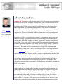
Hi folks, welcome to my personal home page. As you probably already
know, I'm a DSP software developer and full time computer nerd which
basically means that I actually get paid to spend a fair amount of my time in
front of those one-eyed monsters. Although I'm primarily involved in
commercial software development (after all, one has to make a living
somehow) I'm also having a part time commitment to DSP education with
courses mainly for students and software developers confronted with the
task of developing DSP/audio processing systems, held at a local
educational institute. Besides that, I'm writing articles on DSP for some
magazines from time to time (if you're an editor and you'd like me to write
for your magazine, ask me).
.
.
.
So what's this site all about. Basically, I think that I have collected a fair
amount of material during the last years and during my time as researcher
in a non-commercial institution that may be worth sharing on the internet to
people who are interested in learning the concepts of DSP. For those of you
who did not come across this term yet: "DSP" stands for "Digital Signal
Processing" and describes the science that tries to analyze, generate and
manipulate measured real world signals with the help of a digital computer.
These signals can be anything that is a collection of numbers, or
measurements, most commonly used include images, audio (such as
digitally recorded speech and music) and medical and seismic data. Being
involved in education related to specifically audio signal processing
anyway, I see no reason why I shouldn't make some of the stuff I use in my
courses available to the public here.
So, why would I feed my competition for free? Well, you will certainly not
see any proprietary stuff here that I have developed as an employee. I'm
certainly not interested in getting sued or losing my job, or both.
Everything on these pages is from my courses in education - and all I will
do is give you something to play with, and think about. No holy grail here
(if I only had it myself). Finally, if you're still convinced that you need to
take over my job after reading or attending my courses, apply here (no,
really, we're still desperately looking for skilled people to expand our
team).
Again, what's this site all about. This site is dedicated to outlining some
DSP concepts that are commonly underrepresented elsewhere, with a main
focus on music/audio applications. Most other sites of this kind focus on
audio DSP applications that deal with common tasks, such as filter design,
adaptive filtering, the basics of discrete time sampling,
encoding/compression of data, aliasing, Fourier transform theory and
related things. This is mainly due to the fact that these are the tools
frequently needed by DSP people.This site will not cover them at all (er,
almost), since I personally believe there are enough good descriptions of
these topics on the web and in the books and I won't waste the small
amount of time I have on repeating them here. Instead, this site will assume
you are already familiar with (or at least willing to learn) the basics and
start at a reasonably high level. This does not mean that you won't
understand anything if you're a DSP newbie, it simply means I won't
discuss the usual mathematical justifications for doing the things the way I
do them, especially with regard to mathematical constraints such as the
causality of realtime systems and things like error estimation in bandlimited
systems that are discretely and uniformly sampled. Usually, in practice you
will sometimes require them, so you should make yourself familiar with the
concepts at some time. However, for now, these issues are not required.
One exception to this is my "DFT Explained" article. In this article, I will
explain the most important properties and the most frequently asked
questions about the Discrete Fourier Transform, in simple terms. I do this
because I feel that this topic is one of the commonly misunderstood ones,
and I have not found any really satisfactory in-depth explanation of this on
the web yet.
.
.
You will find that from time to time I will need to discuss some maths, but
I'll do my best to keep it as simple as possible and try to do it in a way that
does not clutter the actual content too much. Instead, I will try to focus on
intuitively describing and implementing the things I belabor, and provide
short segments of code that are platform independent and can be used as
'black boxes' to visualize the processes and results.
Besides my own work, you will find hopefully useful links to other
interesting and related sites here, as well as some free applications I
developed during the last few years in my spare time. I will also provide
some source code snippets for some of the applications, which are taken
from my upcoming book (I will announce it officially here when I get it
done). Please see the legal information and notices as well as the terms of
use for the code and applications on the pages where they are provided.
Being my homepage, this site will also have some personal information on
myself, my interests, hobbies and other (un)related stuff.
Important Legal Issues
Please note that all content provided on this web site is strictly for
educational purposes only, which means that I neither take any
responsibility as to the correctness of the references and algorithms nor do I
make any representation as to its usefulness or fitness for a particular
purpose. You, the reader, are taking the full responsibility for the use of the
material. All source code examples have been authored by myself in my
free time with the agreement of my employer, and I did my best to check
that they are not conflicting with the rights of any other parties. I do not get
paid for maintaining this site or providing the content, and I do not
guarantee that through the use of the software and source code examples
provided on this site in a commercial software you do not infringe on any
patent or other means of intellectual property protection of a 3rd party
company. All examples provided are copyrighted material created by
myself and are therefore subject to all applicable copyright regulations in
your country. They may not be reproduced or otherwise used in any context
without my prior written consent. Whenever I need to reference to code
written by other authors, I do my best to cite the references correctly or
provide links to their web site. I will not reproduce any code written by
others on this site without their explicit consent.
last change: 12.08.1999, ©1999 S. M. Sprenger, all rights reserved. Content subject to change without notice. Content
provided 'as is', see disclaimer.
Introduction
The materials ("Materials") contained in Stephan M. Sprenger's ("AUTHOR") web site are
provided by AUTHOR and may be used for informational purposes only. By downloading
any of the Materials contained in any of AUTHOR's sites, you agree to the terms and
provisions as outlined in this legal notice. If you do not agree to them, do not use this site
or download Materials.
Trademark Information
All AUTHOR's product or service names or logos referenced in the AUTHOR's Web site
are either trademarks or registered trademarks of AUTHOR. The absence of a product or
service name or logo from this list does not constitute a waiver of AUTHOR's trademark or
other intellectual property rights concerning that name or logo.
All other products and company names mentioned in the AUTHOR's Web site may be
trademarks of their respective owners.
Use of the AUTHOR's Logos for commercial purposes without the prior written consent of
AUTHOR may constitute trademark infringement and unfair competition in violation of
federal and state laws. Use of any other AUTHOR's trademark in commerce may be
prohibited by law except by express license from AUTHOR.
Mac and the Mac logo are trademarks of Apple Computer, Inc., registered in the U.S. and
other countries. The Made on a Mac Badge is a trademark of Apple Computer, Inc., used
with permission.
Ownership of Materials
The information contained in this site is copyrighted and may not be distributed, modified,
reproduced in whole or in part without the prior written permission of AUTHOR. The
images from this site may not be reproduced in any form without the prior written consent
of AUTHOR.
Software and Documentation Information
Software
Use of the software from this site is subject to the software license terms set forth in the
accompanying Software License. The software license agreement is included with the
software packages available for download from this site.
Documentation
Any person is hereby authorized to: a) store documentation on a single computer for
personal use only and b) print copies of documentation for personal use provided that the
documentation contains AUTHOR's copyright notice.
Third Party Companies and Products
Mention of third-party products, companies and web sites on the AUTHOR's Web site is
for informational purposes only and constitutes neither an endorsement nor a
recommendation. AUTHOR assumes no responsibility with regard to the selection,
performance or use of these products or vendors. AUTHOR provides this only as a
convenience to their users. AUTHOR has not tested any software found on these sites and
makes no representations regarding the quality, safety, or suitability of any software found
there. There are dangers inherent in the use of any software found on the Internet, and
AUTHOR assumes no responsibility with regard to the performance of use of these
products. Make sure that you completely understand the risks before retrieving any
software on the Internet. All third party products, plug ins and software components must
be ordered directly from the vendor, and all licenses and warranties, if any, take place
between you and the vendor.
Links to Other Web Sites
AUTHOR makes no representation whatsoever regarding the content of any other web sites
which you may access from the AUTHOR's Web site. When you access a non- AUTHOR's
web site, please understand that it is independent from AUTHOR and that AUTHOR has
no control over the content on that web site. A link to a non- AUTHOR's web site does not
mean that AUTHOR endorses or accepts any responsibility for the content or use of such
web site.
Feedback and Information
Any feedback you provide at this site shall be deemed to be non-confidential. AUTHOR
shall be free to use such information on an unrestricted basis.
Warranties and Disclaimers
AUTHOR intends for the information and data contained in the AUTHOR's Web site to be
accurate and reliable, however, it is provided "AS IS."
AUTHOR EXPRESSLY DISCLAIMS ALL WARRANTIES AND/OR
CONDITIONS, EXPRESS OR IMPLIED, AS TO ANY MATTER WHATSOEVER
RELATING TO OR REFERENCED BY THE AUTHOR's WEB SITE,
INCLUDING, BUT NOT LIMITED TO, THE IMPLIED WARRANTIES AND/OR
CONDITIONS OF MERCHANTABILITY OR SATISFACTORY QUALITY AND
FITNESS FOR A PARTICULAR PURPOSE AND NON INFRINGEMENT.
last change: 12.08.1999, ©1999 S. M. Sprenger, all rights reserved. Content subject to change without notice. Content provided 'as is',
see disclaimer.
.
August 13th (yes, a Friday), 1999
Registered domain name and allocated disk space. First upload of the basic web
site framework to the server
August 16th, 1999
Added 'Links' page, added 'What's new' section. Checked the links page for
broken links and removed them. Did some minor cosmetic changes.
August 29th, 1999
Added some more links to the 'Links' page. Created a paragraph named
'favourite links'
September 19th, 1999
Fixed some typos on the formant tutorial page
November 3rd, 1999
Upgraded DSP Dimension to provide a higher transfer volume due to the
immense interest. October alone had 114 MB download of web content (not
counting audio) which is overwhelming considering the pages occupied a little
over 700kB at that time.
November 22th, 1999
Finally finished and uploaded the two articles "The DFT à Pied" and "Pitch
Scaling Using The Fourier Transform". Did some other minor corrections
regarding the Meta tags of the pages.
August 29th, 2000
Sorry folks, I'm too busy to put more goodies up here. However, I now managed
to offer the entire website as one PDF download (which is easier than saving
.
each page manually). Also, I did some minor changes to the smsPitchScale code
documentation since I received several questions from you about data format
and units used there.
September 19th, 2000
Did some changes to the HTML code to speed up loading of the pages.
September 21th, 2000
Updated the LINKS page.
December 12th, 2001
Added a link to Rick Bloor's VST Plugin based on DSPdimension code
January 18th, 2002
Added the PICO Search engine and updated the links on the Time/Pitch Scaling
page
August 16th, 2002
Added the Fun Stuff category
December, 2002
Did some minor bug fixing and cleanup of part of the code presented on this site
January 12th, 2003
Added details on my past work and area of expertise
January 27th, 2003
Added the Neuron stuff page with articles, making-of and other stuff to come
soon
last change: 27.01.2003, ©1999-2003 S. M. Sprenger, all rights reserved. Content subject to change without notice.
Content provided 'as is', see disclaimer.
by Stephan M. Sprenger, http://www.dspdimension.com, © 1995-2002 all rights reserved
1.
Introduction
1.1
Pitch Shift vs. Pitch Scale Audio Examples
.
2.
.
Techniques Used for Time/Pitch Scaling
2.1
The Phase Vocoder
2.1.1 Related Topics
2.1.2 Why Phase?
.
2.2
.
Time Domain Harmonic Scaling (TDHS)
2.3
More recent approaches
.
.
3.
Comparison
3.1
Which Method to Use
3.2
Pitch Scaling Considerations
3.3. Audio Examples
.
4.
.
Timbre and Formants
4.1. Phase Vocoder and Formants
4.2. Time Domain Harmonic Scaling and Formants
.
.
1. Introduction
As opposed to the process of pitch transposition achieved using a simple sample rate
conversion, Pitch Scaling is a way to change the pitch of a signal without changing its length.
In practical applications, this is achieved by changing the length of a sound using one of the
below methods and then performing a sample rate conversion to change the pitch. There
exists a certain confusion in terminology, as Pitch Scaling is often also incorrectly named
'Pitch Shift' (a term coined by the music industry). A true Pitch Shift (as obtainable by
modulating an analytic signal by a complex exponential) will shift the spectrum of a sound,
while Pitch Scaling will dilate it, upholding the harmonic relationship of the sound. The
actual Pitch Shifting yields a metallic, inharmonic sound which may well be an interesting
special effect but which is a totally inadequate process for changing the pitch of any
harmonic sound except a single sine wave.
1.1 Audio Examples:
original sound
(WAVE, 106k)
pitch shifted
(WAVE, 106k)
pitch scaled
(WAVE, 106k)
(Read my Audio Example Notes page for more information on how to use the above
examples on your computer)
There are several fairly good methods to do time/pitch scaling but most of them will not
perform well on all different kinds of signals and for any desired amount of scaling.
Typically, good algorithms allow pitch shifting up to 5 semitones on average or stretching
the length by 130%. When time/pitch scaling single instrument recordings you might even be
able to achieve a 200% time scaling, or a one-octave pitch scaling with no audible loss in
quality.
2. Techniques Used for Time/Pitch Scaling
Currently, there are two different principal time/pitch scaling schemes employed in most of
today's applications:
2.1 Phase Vocoder. This method was introduced by Flanagan and Golden in 1966 and
digitally implemented by Portnoff ten years later. It uses a Short Time Fourier Transform
(which we will abbreviate as STFT from here on) to convert the audio signal to the complex
Fourier representation. Since the STFT returns the frequency domain representation of the
signal at a fixed frequency grid, the actual frequencies of the partial bins have to be found by
converting the relative phase change between two STFT outputs to actual frequency changes
(note the term 'partial' has nothing to do with the signal harmonics. In fact, a STFT will never
readily give you any information about true harmonics if you are not matching the STFT
length the fundamental frequency of the signal - and even then is the frequency domain
resolution quite different to what our ear and auditory system perceives). The timebase of the
signal is changed by interpolating and calculating the new frequency changes in the Fourier
domain on a different time basis, and then a iSTFT is done to regain the time domain
representation of the signal.
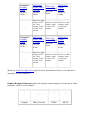
Table 1: Fourier Transform Pointers:
Jean Baptiste Joseph Fourier bio
Discrete Time FT Basics
Dave Hales FFT Laboratory (requires Java capable browser)
S.M.Sprenger's DFT à Pied article (with C code)
Chris Bores' Online DSP Courses
Phase vocoder algorithms are used mainly in scientific and educational software products (to
show the use and limitations of the Fourier Transform ). They have severe drawbacks and
introduce a considerable amount of artifacts audible as 'smearing' and 'reverberation' (even at
low expansion ratios) due to the non-synchronized vertical coherence of the sine and cosine
basis functions and the interpolation that is used to change the timebase.
2.1.1 Related topics
There often is a certain confusion between a 'regular' (channel) and the phase vocoder. Both
of them are different in that they are used to achieve different effects. The channel vocoder
also uses two input signals to produce a single output channel while the phase vocoder has a
one-in, one-out signal path. In the channel vocoder as applied to music processing, the
modulator input signal is split into different filter bands whose amplitudes are modulating the
(usually) corresponding filter bands splitting the carrier signal. More sophisticated (and
expensive) approaches also separate voiced and unvoiced components in the modulator (or,
for historical reasons 'speech') input, i.e. vowels and sibilancies, for independent
processing.The channel vocoder can not be successfully applied to the time/pitch scaling
problem, in musical context it mainly is a device for analyzing and imposing formant
frequencies from one sound on another. Both are similar in that they use filter banks (the
STFT can be seen as a filter bank consisting of steep and slightly overlapping constant
bandwidth filters) but a maximum of 22 are typical for channel vocoders while a phase
vocoder usually employs a minimum of 512 or 1024 filter bands. The term Voice Coder
(Vocoder) refers to the original application of the two processes in speech coding for military
purposes.
2.1.2 Why Phase?
The term 'phase' in phase vocoder refers to the fact that the temporal development of a sound
is contained in its phase information - while the amplitudes just denote that a component is
present in a sound, phase contains the structural information. The phase relationships
between the different bins will reconstruct time-limited events when the time domain
representation is resynthesized. The phase difference of each bin between two successive
analysis frames is used to determine that bin's frequencies deviation from its mid frequency,
thus providing information about the bin's true frequency (if it is not a multiple of the STFT
frame in its period) and thus making a reconstruction on a different time basis possible.
Table 2: Pointers, Phase Vocoder:
The MIT Lab Phase Vocoder
Phase Vocoder References
Richard Dobson's non-mathematical explanation of the Phase Vocoder
(suggested reading!)
Tom Erbe's SoundHack (Macintosh)
The IRCAM "Super Phase Vocoder" (no demo version)
S.M.Sprenger's Pitch Scaling Using The Fourier Transform article
(with C code)
Table 3: Pointers, sinusoidal modelling (Phase Vocoder-related
technique):
SMS sound processing package (incl. executables for several platforms)
Lemur (Mac program along with references and documentation)
Table 4: Pointers, other interesting spectral manipulation tools
Macintosh programs
Windows programs
However, in today's commercial music/audio DSP software you will most likely find the
technique of
2.2 Time Domain Harmonic Scaling (TDHS). This is based on a method proposed by
Rabiner and Schafer in 1978. In one of the numerous possible implementations, the Short
Time Autocorrelation of the signal is taken and the fundamental frequency is found by
picking the maximum (alternatively, one can use the Short Time Average Magnitude
Difference function and find the minimum, which is faster on an average CISC based
computer systems). The timebase is changed by copying the input to the output in an overlapand-add manner (therefore it's also sometimes referred to as 'SOLA' - synchronized overlapadd method) while simultaneously incrementing the input pointer by the overlap-size minus
a multiple of the fundamental frequency. This results in the input being traversed at a
different speed than the original data was recorded at while aligning to the basic period
estimated by the above method. This algorithm works well with signals having a prominent
basic frequency and can be used with all kinds of signals consisting of a single signal source.
When it comes to mixed-source signals, this method will produce satisfactory results only if
the size of the overlapping segments is increased to include a multiple of cycles thus
averaging the phase error over a longer segment making it less audible. For Time Domain
Harmonic Scaling the basic problem is estimating the basic pitch period of the signal,
especially in cases where the actual fundamental frequency is missing. Numerous pitch
estimation algorithms have been proposed and some of them can be found in the following
references:
Table 4: Pointers, TDHS
'C Algorithms for Realtime DSP' by Paul M. Embree, Prentice Hall,
1995 (incl. source code diskette)
'Numerical Recipes in C' by W. Press, S. Teukolsky, W. Vetterling, B.
Flannery, Cambridge University Press, 1988/92 (incl. source code
examples, click title to read it online)
'Digital Processing of Speech Signals' by L.R. Rabiner and
R.W.Schafer, Prentice Hall, 1978 (no source code, covers TDHS
basics)
'An Edge Detection Method for Time Scale Modification of Acoustic
Signals', Rui Ren, Computer Science Department, Hong Kong
University of Science and Technology.
'Time Stretch & Pitch Shift - breaking the 10% barrier', Centre for
Communications Research, Digital Music Research Group
'Dichotic time compression and spatialization' by Barry Arons, MIT
Media Laboratory
Other papers related to Time Compression/Expansion by Barry Arons,
MIT Media Lab
2.3 More recent approaches. Due to the huge amount of artifacts produced by both of the
above methods, there have been a number of more advanced approaches to the problem of
time and pitch scaling in the past years. One particular problem of both the TDHS and Phase
Vocoder approaches is the high localization of the basis functions (where this term is
applicable) in one domain with no localization in the other. The sines and cosines used in the
Phase Vocoder have no localization in the Time Domain, which without further treatment
contributes to the inherent signal smearing. The sample snippets used in the TDHS approach
can be seen as having no localization in the frequency domain, thus causing multi-pitched
signals to produce distortion. A method which was developed by Prosoniq uses an approach
of representing the signal in terms of more complex basis functions that have a good
localization in both the time and frequency domain (like certain types of wavelets have). The
signal is transformed on the basis of the proprietary MCFE (Multiple Component Feature
Extraction), which shall not be discussed here.
Table 5: Pointers, More recent approaches
The Prosoniq MPEX Time/Pitch Scaling technology (licensing of
binary object code)
Time/Pitch Scaling Using The Constant-Q Phase Vocoder, J. Garas, P.
Sommen, Eindhoven University of Technology, The Netherlands
Scott Levine, Tony Verma, Julius O. Smith III. Alias-Free,
Multiresolution Sinusoidal Modeling for Polyphonic, Wideband Audio.
IEEE Workshop on Applications of Signal Processing to Audio and
Acoustics, Mohnonk, NY, 1997.
Scott Levine, Julius O. Smith III. A Sines+Transients+Noise Audio
Representation for Data Compression and Time/Pitch-Scale
Modifications. 105th Audio Engineering Society Convention, San
Francisco 1998.
3. Comparison
We have produced a small number of audio examples as well as some screen shots of
impulse responses to show the performance in quality of each method in comparison.
3.1 Which Method To Use. Principally, this is dependent on the constraints imposed on the
actual task, which may be one of the following:
Speed. If you plan on using the method in a realtime application, TDHS is probably the best
option unless you have a STFT representation of the signal already at hand. Using different
optimization techniques, the performance of this approach can be fine tuned to run on almost
any of today's computer in realtime.
Material. If you have a prior knowledge about the signal the algorithm is supposed to work
well with, you can further choose and optimize your algorithm accordingly (see below).
Quality. If the ultimate goal of your application is to provide the highest possible quality
without performance restrictions, you should decide with the following two important factors
in mind: 1) TDHS gives better results for small timebase and pitch changes, but will not
work well with most polyphonic material. 2) Phase Vocoder gives smoother results for larger
changes and will also work well with polyphonic material but introduces signal smearing
with impulsive signals.
3.2 Pitch Scaling Considerations: If your goal is to alter the pitch, not the timebase, bear in
mind that when upscaling the pitch, echoes andthe repetituous behaviour of TDHS are less
obvious since the pitch change moves adjacent peaks (echoes) closer to each other in time,
thus masking them to the ear. The pre-smearing behaviour of the Phase Vocoder will be
more disturbing in this case, since it occurs before the transient sounds and will easily be
recognized by the listener.
3.3 Audio Examples:
Example 1:
original
sound
(WAVE,
106k)
--
Example 2:
original
sound
(WAVE,
230k)
--
200% time
scaled, Phase
Vocoder
(WAVE,
209k)
200% time
200% time
scaled,
scaled, TDHS
MCFE
(WAVE,
(WAVE,
209k)
209k)
block size: 2048
samples, STFT
size: 8192
samples, frame
overlap: 1024
samples
block size: 2048
samples, frame
overlap: 1536
samples
200% time
scaled, Phase
Vocoder
(WAVE,
432k)
200% time
200% time
scaled,
scaled, TDHS
MCFE
(WAVE,
(WAVE,
451k)
451k)
block size: 2048
samples, STFT
size: 8192
samples, frame
overlap: 1024
samples
block size: 2048
samples, frame
overlap: 1536
samples
block size: 1806
samples, frame
overlap: 903
samples
block size: 1806
samples, frame
overlap: 903
samples
(Read my Audio Example Notes page for more information on how to use the above
examples on your computer)
Impulse Response Diagrams (achieved using the same settings as for the above audio
examples, click to view in detail):
Original
Phase Vocoder
TDHS
MCFE
4. Timbre and Formants
Since timbre (formant) manipulation is actually a pitch scaling related topic, it will also be
discussed here. Formants are prominent frequency regions produced by the resonances in the
instrument's body that very much determine the timbre of a sound. For human voice, they
come from the resonances and cancellations of the vocal tract, contributing to the specific
characteristics of a speaker's and singer's voice.
If the pitch of a recording is scaled, formants will be moved thus producing the well known
'Mickey-Mouse' effect audible when scaling the pitch. This is usually an unwanted side
effect since the formants of a human singing at a higher pitch do not change their position.
To compensate for this, there exist formant correction algorithms that restore the position of
the formant frequencies after or during the pitch scaling process. They also allow changing
the gender of a singer by scaling formants without changing pitch.
For each of the above time/pitch scaling method there exists a corresponding method for
changing the formants to compensate for the side effects of the transposition.
4.1 Phase Vocoder and Formants. Formant manipulation in the STFT representation can be
done by first normalizing the spectral amplitude envelope and then multiplying it by a nonpitch scaled copy of it. This removes the new formant information generated through the
pitch scaling and superimposes the original formant information thus yielding a sound
similar to the original voice. This is an amplitude-only operation in the frequency domain
and therefore does not involve great additional computational complexity. However, the
quality may not be optimal in all cases.
4.2 Time Domain Harmonic Scaling and Formants. Changing the formants in the time
domain is simple, however, efficient implementation is tricky. TDHS in essence can be
implemented and regarded as a granular synthesis using grains of one cycle of the
fundamental in length being output at the destination new fundamental frequency rate.
Simply put: if each grain is 1 cycle in length and since [cycles/sec] is the definition of
fundamental pitch in this case, the output rate of these grains determines the new pitch of the
sample. In order to not lengthen the sample, some grains have to be discarded in the process.
Since no transposition takes place, the formants will not move. On the other hand, applying a
sample rate change to the grains results in a change of formants without affecting the pitch.
Thus, pitch and formants can be independently moved. The obvious disadvantage of the
process is its dependency on the fundamental frequency of the signal, making it unsuited for
the application to polyphonic material. See also: 'A Detailed Analysis of a Time-Domain
Formant-Corrected Pitch-Shifting Algorithm', by Robert Bristow-Johnson, Journal of the
Audio Engineering Society, May 1995. This paper discusses an algorithm previously
proposed by Keith Lent in the Computer Music Journal.
Table 6: Pointers, Formant Manipulation
The DSP Dimension Formant Correction page.
An LPC Approach: 'Voice Gender Transformation with a Modified
Vocoder' (May 1996), Yoon Kim at CCRMA
The following newsgroups can be acessed for more information and help on the time/pitch
scaling topic.
Table 7: News Groups
comp.dsp
comp.music.research
If you're seeking general information on DSP, browse to the DSPguru homepage.
last change: 18.01.2002, ©1999-2002 S. M. Sprenger, all rights reserved. Content subject to change without notice. Content provided
'as is', see disclaimer.
by Stephan M. Sprenger, http://www.dspdimension.com, © 1995-99 all rights reserved
1.
Introduction
1.1
What are formants?
1.2
Audio Example - original
1.3
Why formants change with transposition
1.4
Audio Example - pitch scaled, formants change
1.5
Why singer formants do not change
1.6
Audio Example - pitch scaled, formants do not change
.
.
1. Introduction
This page is dedicated exclusively to the topic of formant movement occuring when pitch
scaling sampled sounds. It will detail the effects involved and show pictures of the effects
that cause unnatural sounding pitch scales.
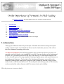
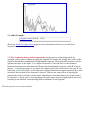
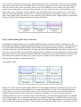
1.1 What are formants? The following graphics shows a short time fourier spectrum of a
sampled sound of a female voice singing the vowel 'ah'. One can clearly see the fundamental
frequency as a prominent peak to the left side of the display. The individual harmonics can
be seen as small peaks of varying amplitude forming a regular pattern with equal distances to
the fundamental frequency. To the right of the fundamental frequency one could see the
harmonics forming some small peaks connected with a dotted line beneath a larger section
marked with a solid line and the letter F. The small peaks and the large peak are all formants,
we have marked the widest formant with F for utmost clarity and visibility.
Click the picture to view more details.
1.2 Audio Example:
original sound (WAVE, 132k)
(Read my Audio Example Notes page for more information on how to use the above
example on your computer)
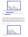
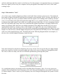
1.3 Why formants change with transposition. In the process of upscaling pitch for
example, either with or without keeping the original file length, the sample rate of the audio
signal is altered thus expanding the fundamental frequency along with all harmonics and the
spectral envelope to the right, i.e. to higher frequencies. One can also see the distances
between the harmonics determined by N times the fundamental frequency (with N being an
integer > 1) becoming larger as is typical for a higher pitch (this would not be the case if you
had really shifted the pitch). As the spectral envelope (and thus the marked position F) is also
stretched, the position of the formants is altered. This has the same effect as altering the
proportions of the vocal tract of the singer, shrinking or stretching him in size from a dwarf
to a monster. Clearly, this is not happening when the singer sings at a higher pitch, therefore
resulting in an artificial sound bearing little resemblance to the original.
Click the picture to view more details.
1.4 Audio Example:
pitch scaled, formants move (WAVE, 132k)
(Read my Audio Example Notes page for more information on how to use the above
example on your computer)
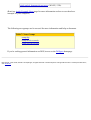
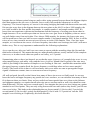
1.5 Why singer formants do not change. When keeping the spectral envelope, i.e. the
position of the formants either by pitch transposing with Timbre Correction or by having the
singer sing at a higher pitch, one yields a natural sounding transpose. As shown below, the
position of the formants (and the marked region F) is not altered during the process of
singing at different pitches although the relative distances between the harmonics are now
different. When singing at a higher pitch, the formants are not changed since the vocal tract
responsible for resonances and cancellations forming the formants also remains unchanged.
Click the picture to view more details.
1.6 Audio Example:
pitch scaled, formants do not move (WAVE, 132k)
(Read my Audio Example Notes page for more information on how to use the above
example on your computer)
The following newsgroups can be acessed for more information and help on formants.
Table 7: News Groups
comp.dsp
comp.music.research
comp.speech.research
If you're seeking general information on DSP, browse to the DSPguru homepage.
last change: 19.09.1999, ©1999 S. M. Sprenger, all rights reserved. Content subject to change without notice. Content provided 'as is',
see disclaimer.
.
by Stephan M. Sprenger, http://www.dspdimension.com, © 1999 all rights reserved*
If you're into signal processing, you will no doubt say that the headline is a very tall claim. I would
second this. Of course you can't learn all the bells and whistles of the Fourier transform in one day
without practising and repeating and eventually delving into the maths. However, this online course will
provide you with the basic knowledge of how the Fourier transform works, why it works and why it can
be very simple to comprehend when we're using a somewhat unconventional approach.The important
part: you will learn the basics of the Fourier transform completely without any maths that goes beyond
adding and multiplying numbers! I will try to explain the Fourier transform in its practical application to
audio signal processing in no more than six paragraphs below.
Step 1: Some simple prerequisites
What you need to understand the following paragraphs are essentially four things: how to add numbers,
how to multiply and divide them and what a sine, a cosine and a sinusoid is and how they look.
Obviously, I will skip the first two things and just explain a bit the last one. You probably remember
from your days at school the 'trigonometric functions'1 that were somehow mysteriously used in
conjunction with triangles to calculate the length of its sides from its inner angles and vice versa. We
don't need all these things here, we just need to know how the two most important trigonometric
functions, the "sine" and "cosine" look like. This is quite simple: they look like very simple waves with
peaks and valleys in them that stretch out to infinity to the left and the right of the observer.
The sine wave
The cosine wave
As you can see, both waves are periodic, which means that after a certain time, the period, they look the
same again. Also, both waves look alike, but the cosine wave appears to start at its maximum, while the
sine wave starts at zero. Now in practice, how can we tell whether a wave we observe at a given time
started out at its maximum, or at zero? Good question: we can't. There's no way to discern a sine wave
and a cosine wave in practice, thus we call any wave that looks like a sine or cosine wave a "sinusoid",
which is Greek and translates to "sinus-like". An important property of sinusoids is "frequency", which
tells us how many peaks and valleys we can count in a given period of time. High frequency means many
peaks and valleys, low frequency means few peaks and valleys:
Low frequency
sinusoid
Middle frequency
sinusoid
High frequency
sinusoid
Step 2: Understanding the Fourier Theorem
Jean-Baptiste Joseph Fourier was one of those children parents are either proud or ashamed of, as he
started throwing highly complicated mathematical terms at them at the age of fourteen. Although he did a
lot of important work during his lifetime, the probably most significant thing he discovered had to do
with the conduction of heat in materials. He came up with an equation that described how the heat would
travel in a certain medium, and solved this equation with an infinite series of trigonometric functions (the
sines and cosines we have discussed above). Basically, and related to our topic, what Fourier discovered
boils down to the general rule that every signal, however complex, can be represented by a sum of
sinusoid functions that are individually mixed.
An example of this:
This is our original
One sine
Two sines
Four sines
Seven sines
Fourteen sines
What you see here is our original signal, and how it can be approximated by a mixture of sines (we will
call them partials) that are mixed together in a certain relationship (a 'recipe'). We will talk about that
recipe shortly. As you can see, the more sines we use the more accurately does the result resemble our
original waveform. In the 'real' world, where signals are continuous, ie. you can measure them in
infinitely small intervals at an accuracy that is only limited by your measurement equipment, you would
need infinitely many sines to perfectly build any given signal. Fortunately, as DSPers we're not living in
such a world. Rather, we are dealing with samples of such 'realworld' signals that are measured at regular
intervals and only with finite precision. Thus, we don't need infinitely many sines, we just need a lot. We
will also talk about that 'how much is a lot' later on. For the moment, it is important that you can imagine
that every signal you have on your computer can be put together from simple sine waves, after some
cooking recipe.
Step 3: How much is "a lot"
As we have seen, complex shaped waveforms can be built from a mixture of sine waves. We might ask
how many of them are needed to build any given signal on our computer. Well, of course, this may be as
few as one single sine wave, provided we know how the signal we are dealing with is made up. In most
cases, we are dealing with realworld signals that might have a very complex structure, so we do not know
in advance how many 'partial' waves there are actually present. In this case, it is very reassuring to know
that if we don't know how many sine waves constitute the original signal there is an upper limit to how
many we will need. Still, this leaves us with the question of how many there actually are. Let's try to
approach this intuitively: assume we have 1000 samples of a signal. The sine wave with the shortest
period (ie. the most peaks and valleys in it) that can be present has alternating peaks and valleys for every
sample. So, the sine wave with the highest frequency has 500 peaks and 500 valleys in our 1000 samples,
with every other sample being a peak. The black dots in the following diagram denote our samples, so
the sine wave with the highest frequency looks like this:
The highest frequency sine
wave
Now let's look how low the lowest frequency sine wave can be. If we are given only one single sample
point, how would we be able to measure peaks and valleys of a sine wave that goes through this point?
We can't, as there are many sine waves of different periods that go through this point.
Many sine waves go through one
single point, so one point doesn't tell
us about frequency
So, a single data point is not enough to tell us anything about frequency. Now, if we were given two
samples, what would be the lowest frequency sine wave that goes through these two points? In this case,
it is much simpler. There is one very low frequency sine wave that goes through the two points. It looks
like this:
The lowest frequency sine wave
Imagine the two leftmost points being two nails with a string spanned between them (the diagram depicts
three data points as the sine wave is periodic, but we really only need the leftmost two to tell its
frequency). The lowest frequency we can see is the string swinging back and forth between the two nails,
like our sine wave does in the diagram between the two points to the left. If we have 1000 samples, the
two 'nails' would be the first and the last sample, ie. sample number 1 and sample number 1000. We
know from our experience with musical instruments that the frequency of a string goes down when its
length increases. So we would expect that our lowest sine wave gets lower in frequency when we move
our nails farther away from each other. If we choose 2000 samples, for instance, the lowest sine wave
will be much lower since our 'nails' are now sample number 1 and sample number 2000. In fact, it will be
twice as low, since our nails are now twice as far away as in the 1000 samples. Thus, if we have more
samples, we can discern sine waves of a lower frequency since their zero crossings (our 'nails') will move
farther away. This is very important to understand for the following explanations.
As we can also see, after two 'nails' our wave starts to repeat with the ascending slope (the first and the
third nail are identical). This means that any two adjacent nails embrace exactly one half of the complete
sine wave, or in other words either one peak or one valley, or 1/2 period.
Summarizing what we have just learned, we see that the upper frequency of a sampled sine wave is every
other sample being a peak and a valley and the lower frequency bound is half a period of the sine wave
which is just fitting in the number of samples we are looking at. But wait - wouldn't this mean that while
the upper frequency remains fixed, the lowest frequency would drop when we have more samples?
Exactly! The result of this is that we will need more sine waves when we want to put together longer
signals of unknown content, since we start out at a lower frequency.
All well and good, but still we don't know how many of these sine waves we finally need. As we now
know the lower and upper frequency any partial sine wave can have, we can calculate how many of them
fit in between these two limits. Since we have nailed our lowest partial sine wave down to the leftmost
and rightmost samples, we require that all other sine waves use these nails as well (why should we treat
them differently? All sine waves are created equal!). Just imagine the sine waves were strings on a guitar
attached to two fixed points. They can only swing between the two nails (unless they break), just like our
sine waves below. This leads to the relationship that our lowest partial (1) fits in with 1/2 period, the
second partial (2) fits in with 1 period, the third partial (3) fits in with 1 1/2 period asf. into the 1000
samples we are looking at. Graphically, this looks like this:
The first 4 partial sine waves (click to
enlarge)
Now if we count how many sine waves fit in our 1000 samples that way, we will find that we need
exactly 1000 sine waves added together to represent the 1000 samples. In fact, we will always find that
we need as many sine waves as we had samples.
Step 4: About cooking recipes
In the previous paragraph we have seen that any given signal on a computer can be built from a mixture
of sine waves. We have considered their frequency and what frequency the lowest and highest sine
waves need to have to perfectly reconstruct any signal we analyze. We have seen that the number of
samples we are looking at is important for determining the lowest partial sine wave that is needed, but we
have not yet discussed how the actual sine waves have to be mixed to yield a certain result. To make up
any given signal by adding sine waves, we need to measure one additional aspect of them. As a matter of
fact, frequency is not the only thing we need to know. We also need to know the amplitude of the sine
waves, ie. how much of each sine wave we need to mix together to reproduce our input signal. The
amplitude is the height of the peaks of a sine wave, ie. the distance between the peak and our zero line.
The higher the amplitude, the louder it will sound when we listen to it. So, if you have a signal that has
lots of bass in it you will no doubt expect that there must be a greater portion of lower frequency sine
waves in the mix than there are higher frequency sine waves. So, generally, the low frequency sine waves
in a bassy sound will have a higher amplitude than the high frequency sine waves. In our analysis, we
will need to determine the amplitude of each partial sine wave to complete our recipe.
Step 5: About apples and oranges
If you are still with me, we have almost completed our journey towards the Fourier transform. We have
learned how many sine waves we need, that this number depends on the number of samples we are
looking at, that there is a lower and upper frequency boundary and that we somehow need to determine
the amplitude of the individual partial waves to complete our recipe. We're still not clear, however, on
how we can determine the actual recipe from our samples. Intuitively, we would say that we could find
the amplitudes of the sine waves somehow by comparing a sine wave of known frequency to the samples
we have measured and find out how 'equal' they are. If they are exactly equal, we know that the sine
wave must be present at the same amplitude, if we find our signal to not match our reference sine wave at
all we would expect this frequency not to be present. Still, how could we effectively compare a known
sine wave with our sampled signal? Fortunately, DSPers have already figured out how to do this for you.
In fact, this is as easy as multipling and adding numbers - we take the 'reference' sine wave of known
frequency and unit amplitude (this just means that it has an amplitude of 1, which is exactly what we get
back from the sin() function on our pocket calculator or our computer) and multiply it with our signal
samples. After adding the result of the multiplication together, we will obtain the amplitude of the partial
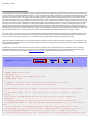
sine wave at the frequency we are looking at. To illustrate this, here's a simple C code fragment that does
this:
Listing 1.1: The direct realization of the Discrete Sine Transform (DST):
#define M_PI 3.14159265358979323846
long bin,k;
double arg;
for (bin = 0; bin < transformLength; bin++) {
transformData[bin] = 0.;
for (k = 0; k < transformLength; k++) {
arg = (float)bin * M_PI *(float)k / (float)transformLength;
transformData[bin] += inputData[k] * sin(arg);
}
}
This code segment transforms our measured sample points that are stored in
inputData[0...transformLength-1] into an array of amplitudes of its partial sine waves
transformData[0...transformLength-1]. According to common terminology, we call the
frequency steps of our reference sine wave bins, which means that they can be thought of as being
'containers' in which we put the amplitude of any of the partial waves we evaluate. The Discrete Sine
Transform (DST) is a generic procedure that assumes we have no idea what our signal looks like,
otherwise we could use a more efficient method for determining the amplitudes of the partial sine waves
(if we, for example, know beforehand that our signal is a single sine wave of known frequency we could
directly check for its amplitude without calculating the whole range of sine waves. An efficient approach
for doing this based on the Fourier theory can be found in the literature under the name the "Goertzel"
algorithm).
For those of you who insist on an explanation for why we calculate the sine transform that way: As a
very intuitive approach to why we multiply with a sine wave of known frequency, imagine that this
corresponds roughly to what in the physical world happens when a 'resonance' at a given frequency takes
place in a system. The sin(arg) term is essentially a resonator that gets excited by our input
waveform. If the input has a partial at the frequency we're looking at, its output will be the amplitude of
the resonance with the reference sine wave. Since our reference wave is of unit amplitude, the output is a
direct measure of the actual amplitude of the partial at that frequency. Since a resonator is nothing but a
simple filter, the transform can (admittedly under somewhat relaxed conditions) be seen as a having the
features of a bank of very narrow band pass filters that are centered around the frequencies we're
evaluating. This helps explaining the fact why the Fourier transform provides an efficient tool for
performing filtering of signals.
Just for the sake of completeness: of course, the above routine is invertible, our signal can (within the
limits of our numerical precision) be perfectly reconstructed when we know its partial sine waves, by
simply adding sine waves together. This is left as an exercise to the reader. The same routine can be
changed to work with cosine waves as basis functions - we simply need to change the sin(arg) term
to cos(arg) to obtain the direct realization of the Discrete Cosine Transform (DCT).
Now, as we have discussed in the very first paragraph of this article, in practice we have no way to
classify a measured sinus-like function as sine wave or cosine wave. Instead we are always measuring
sinusoids, so both the sine and cosine transform are of no great use when we are applying them in
practice, except for some special cases (like image compression where each image might have features
that are well modelled by a cosine or sine basis function, such as large areas of the same color that are
well represented by the cosine basis function). A sinusoid is a bit more general than the sine or cosine
wave in that it can start at an arbitrary position in its period. We remember that the sine wave always
starts out at zero, while the cosine wave starts out at one. When we take the sine wave as reference, the
cosine wave starts out 1/4th later in its period. It is common to measure this offset in degree or radians,
which are two units commonly used in conjunction with trigonometric functions. One complete period
equals 360° (pron. "degree") or 2π radian (pron. "two pi" with "pi" pronounced like the word "pie". π is a
Greek symbol for the number ♠ 3.14159265358979323846... which has some significance in
trigonometry). The cosine wave thus has an offset of 90° or π/2. This offset is called the phase of a
sinusoid, so looking at our cosine wave we see that it is a sinusoid with a phase offset of 90° or π/2
relative to the sine wave.
So what's this phase business all about. As we can't restrict our signal to start out at zero phase or 90°
phase all the time (since we are just observing a signal which might be beyond our control) it is of
interest to determine its frequency, amplitude and phase to uniquely describe it at any one time instant.
With the sine or cosine transform, we're restricted to zero phase or 90° phase and any sinusoid that has an
arbitrary phase will cause adjacent frequencies to show spurious peaks (since they try to 'help' the
analysis to force-fit the measured signal to a sum of zero or 90° phase functions). It's a bit like trying to
fit a round stone into a square hole: you need smaller round stones to fill out the remaining space, and
even more even smaller stones to fill out the space that is still left empty, and so on. So what we need is a
transform that is general in that it can deal with signals that are built of sinusoids of arbitrary phase.
Step 6: The Discrete Fourier transform.
The step from the sine transform to the Fourier transform is simple, making it in a way more 'general'.
While we have been using a sine wave for each frequency we measure in the sine transform, we use both
a sine and a cosine wave in the Fourier transform. That is, for any frequency we are looking at we
'compare' (or 'resonate') our measured signal with both a cosine and a sine wave of the same frequency. If
our signal looks much like a sine wave, the sine portion of our transform will have a large amplitude. If it
looks like a cosine wave, the cosine part of our transform will have a large amplitude. If it looks like the
opposite of a sine wave, that is, it starts out at zero but drops to -1 instead of going up to 1, its sine
portion will have a large negative amplitude. It can be shown that the + and - sign together with the sine
and cosine phase can represent any sinusoid at the given frequency2.
Listing 1.2: The direct realization of the Discrete Fourier Transform3:
#define M_PI 3.14159265358979323846
long bin, k;
double arg, sign = -1.; /* sign = -1 -> FFT, 1 -> iFFT */
for (bin = 0; bin <= transformLength/2; bin++) {
cosPart[bin] = (sinPart[bin] = 0.);
for (k = 0; k < transformLength; k++) {
arg = 2.*(float)bin*M_PI*(float)k/(float)transformLength;
sinPart[bin] += inputData[k] * sign * sin(arg);
cosPart[bin] += inputData[k] * cos(arg);
}
}
We're still left with the problem of how to get something useful out of the Fourier Transform. I have
claimed that the benefit of the Fourier transform over the Sine and Cosine transform is that we are
working with sinusoids. However, we don't see any sinusoids yet, there are still only sines and cosines.
Well, this requires an additional processing step:
Listing 1.3: Getting sinusoid frequency, magnitude and phase from the Discrete Fourier
Transform:
long bin;
double pi = 4.*atan(1.);
for (bin = 0; bin <= transformLength/2; bin++) {
/* frequency */
frequency[bin] = (float)bin * sampleRate /
(float)transformLength;
/* magnitude */
magnitude[bin] = 20. * log10( 2. *
sqrt(sinPart[bin]*sinPart[bin] +
cosPart[bin]*cosPart[bin]) /
(float)transformLength);
/* phase */
phase[bin] = 180.*atan2(sinPart[bin], cosPart[bin])
/ pi - 90.;
}
After running the code fragment shown in Listing 1.3 on our DFT output, we end up with a
representation of the input signal as a sum of sinusoid waves. The k-th sinusoid is described by
frequency[k], magnitude[k] and phase[k]. Units are Hz (Hertz, periods per seconds), dB
(Decibel) and ° (Degree). Please note that after the post-processing of Listing 1.3 that converts the sine
and cosine parts into a single sinusoid, we name the amplitude of the k-th sinusoid the DFT bin
"magnitude", as it will now always be a positive value. We could say that an amplitude of -1.0
corresponds to a magnitude of 1.0 and a phase of either + or -180°. In the literature, the array
magnitude[] is called the Magnitude Spectrum of the measured signal, the array phase[] is called
the Phase Spectrum of the measured signal at the time where we take the Fourier transform.
As a reference for measuring the bin magnitude in decibels, our input wave is expected to have sample
values in the range [-1.0, 1.0), which corresponds to a magnitude of 0dB digital full scale (DFS). As an
interesting application of the DFT, listing 1.3 can, for example, be used to write a spectrum analyzer
based on the Discrete Fourier Transform.
Conclusion
As we have seen, the Fourier transform and its 'relatives', the discrete sine and cosine transform provide
handy tools to decompose a signal into a bunch of partial waves. These are either sine or cosine waves,
or sinusoids (described by a combination of sine and cosine waves). The advantage of using both the sine
and cosine wave simultaneously in the Fourier transform is that we are thus able to introduce the concept
of phase which makes the transform more general in that we can use it to efficiently and clearly analyze
sinusoids that are neither a pure sine or cosine wave, and of course other signals as well.
The Fourier transform is independent of the signal under examination in that it requires the same number
of operations no matter if the signal we are analyzing is one single sinusoid or something else more
complicated. This is the reason why the Discrete Fourier transform is called a nonparametric transform,
meaning that it is not directly helpful when an 'intelligent' analysis of a signal is needed (in the case
where we are examining a signal that we know is a sinusoid, we would prefer just getting information
about its phase, frequency and magnitude instead of a bunch of sine and cosine waves at some predefined
frequencies).
We now also know that we are evaluating our input signal at a fixed frequency grid (our bins) which may
have nothing to do with the actual frequencies present in our input signal. Since we choose our reference
sine and cosine waves (almost) according to taste with regard to their frequency, the grid we impose on
our analysis is artificial. Having said this, it is immediately clear that one will easily encounter a scenario
where the measured signal's frequencies may come to lie between the frequencies of our transform bins.
Consequently, a sinusoid that has a frequency that happens to lie between two frequency 'bins' will not be
well represented in our transform. Adjacent bins that surround the bin closest in frequency to our input
wave will try to 'correct' the deviation in frequency and thus the energy of the input wave will be
smeared over several neighbouring bins. This is also the main reason why the Fourier transform will not
readily analyze a sound to return with its fundamental and harmonics (and this is also why we call the
sine and cosine waves partials, and not harmonics, or overtones).
Simply speaking, without further post-processing, the DFT is little more than a bank of narrow, slightly
overlapping band pass filters ('channels') with additional phase information for each channel. It is useful
for analyzing signals, doing filtering and applying some other neat tricks (changing the pitch of a signal
without changing its speed is one of them explained in a different article on DSPdimension.com), but it
requires additional post processing for less generic tasks. Also, it can be seen as a special case of a family
of transforms that use basis functions other than the sine and cosine waves. Expanding the concept in this
direction is beyond the scope of this article.
Finally, it is important to mention that there is a more efficient implementation of the DFT, namely an
algorithm called the "Fast Fourier Transform" (FFT) which was originally conceived by Cooley and
Tukey in 1969 (its roots however go back to the work of Gauss and others). The FFT is just an efficient
algorithm that calculates the DFT in less time than our straightforward approach given above, it is
otherwise identical with regard to its results. However, due to the way the FFT is implemented in the
Cooley/Tukey algorithm it requires that the transform length be a power of 2. In practice, this is an
acceptable constraint for most applications. The available literature on different FFT implementations is
vast, so suffice it to say that there are many different FFT implementations, some of which do not have
the power-of-two restriction of the classical FFT. An implementation of the FFT is given by the routine
smsFft() in Listing 1.4 below.
Listing 1.4: The Discrete Fast Fourier Transform (FFT):
#define M_PI 3.14159265358979323846
void smsFft(float *fftBuffer, long fftFrameSize, long sign)
/*
FFT routine, (C)1996 S.M.Sprenger. Sign = -1 is FFT, 1
is iFFT (inverse)
Fills fftBuffer[0...2*fftFrameSize-1] with the Fourier
transform of the time domain data in
fftBuffer[0...2*fftFrameSize-1]. The FFT array takes and
returns the cosine and sine parts in an interleaved
manner, ie. fftBuffer[0] = cosPart[0], fftBuffer[1] =
sinPart[0], asf. fftFrameSize must be a power of 2. It
expects a complex input signal (see footnote 2), ie.
when working with 'common' audio signals our input
signal has to be passed as
{in[0],0.,in[1],0.,in[2],0.,...} asf. In that case, the
transform of the frequencies of interest is in
fftBuffer[0...fftFrameSize].
*/
{
float wr, wi, arg, *p1, *p2, temp;
float tr, ti, ur, ui, *p1r, *p1i, *p2r, *p2i;
long i, bitm, j, le, le2, k;
for (i = 2; i < 2*fftFrameSize-2; i += 2) {
for (bitm = 2, j = 0; bitm < 2*fftFrameSize; bitm <<= 1) {
if (i & bitm) j++;
j <<= 1;
}
if (i < j) {
p1 = fftBuffer+i; p2 = fftBuffer+j;
temp = *p1; *(p1++) = *p2;
*(p2++) = temp; temp = *p1;
*p1 = *p2; *p2 = temp;
}
}
for (k = 0, le = 2; k < (long)(log(fftFrameSize)/log(2.));
k++) {
le <<= 1;
le2 = le>>1;
ur = 1.0;
ui = 0.0;
arg = M_PI / (le2>>1);
wr = cos(arg);
wi = sign*sin(arg);
for (j = 0; j < le2; j += 2) {
p1r = fftBuffer+j; p1i = p1r+1;
p2r = p1r+le2; p2i = p2r+1;
for (i = j; i < 2*fftFrameSize; i += le) {
tr = *p2r * ur - *p2i * ui;
ti = *p2r * ui + *p2i * ur;
*p2r = *p1r - tr; *p2i = *p1i - ti;
*p1r += tr; *p1i += ti;
p1r += le; p1i += le;
p2r += le; p2i += le;
}
tr = ur*wr - ui*wi;
ui = ur*wi + ui*wr;
ur = tr;
}
}
}
1 simply speaking, trigonometric functions are functions that are used to calculate the angles in a triangle ("tri-gonos" = Greek for
"three corners") from the length of its sides, namely sinus, cosinus, tangent and the arcus tangent. The sinus and cosinus functions
are the most important ones, as the tangent and arcus tangent can be obtained from sinus and cosinus relationships alone.
2 Note that in the literature, due to a generalization that is made for the Fourier transform to work with another type of input signal
called a 'complex signal' (complex in this context refers to a certain type of numbers rather than to an input signal that has a complex
harmonic structure), you will encounter the sine and cosine part under the name 'real' (for the cosine part) and 'imaginary' part (for the
sine part).
3 if you're already acquainted with the DFT you may have noted that this is actually an implementation of the "real Discrete Fourier
Transform", as it uses only real numbers as input and does not deal with negative frequencies: in the real DFT positive and negative
frequencies are symmetric and thus redundant. This is why we're calculating only almost half as many bins than in the sine transform
(we calculate one additional bin for the highest frequency, for symmetry reasons).
Last change: 29.11.1999, ©1999 S. M. Sprenger, all rights reserved. Content subject to change without notice. Content provided 'as is',
see disclaimer. Graphs made using Algebra Graph, MathPad, sonicWORX and other software. Care has been taken to describe
everything as simple yet accurate as possible. If you find errors, typos and ambiguous descriptions in this article, please notify me and I
will correct or further outline them.
Special thanks to Richard Dobson for providing immensely useful suggestions and corrections to my incomplete knowledge of the
English language.
.
by Stephan M. Sprenger, http://www.dspdimension.com, © 1999 all rights reserved*
With the increasing speed of todays desktop computer systems, a growing number of computationally intense tasks such
as computing the Fourier transform of a sampled audio signal have become available to a broad base of users. Being a
process traditionally implemented on dedicated DSP systems or rather powerful computers only available to a limited
number of people, the Fourier transform can today be computed in real time on almost all average computer systems.
Introducing the concept of frequency into our signal representation, this process appears to be well suited for the
rather specialized application of changing the pitch of an audio signal while keeping its length constant, or changing
its length while retaining its original pitch. This application is of considerable practical use in todays audio processing
systems. One process that implements this has been briefly mentioned in our Time/Pitch Scaling introductory course,
namely the "Phase Vocoder". Based on the representation of a signal in the "frequency domain", we will explicitely
discuss the process of pitch scaling1 in this article, under the premise that time scaling is analogous. Usually, pitch
scaling with the Phase Vocoder is implemented by scaling the time base of the signal and using a sample rate
conversion on the output to achieve a change in pitch while retaining duration. Also, some implementations use
explicite additive oscillator bank resynthesis for pitch scaling, which is usually rather inefficient. We will not reproduce
the Phase Vocoder in its known form here, but we will use a similar process to directly change the pitch of a Fourier
transformed signal in the frequency domain while retaining the original duration. The process we will describe below
uses an FFT / iFFT transform pair to implement pitch scaling and automatically incorporates appropriate anti-aliasing
in the frequency domain. A C language implementation of this process is provided in a black-box type routine that is
easily included in an existing development setup to demonstrate the effects discussed.
1. The Short Time Fourier transform
As we have seen in our introductory course on the Fourier transform, any sampled signal can be represented by a
mixture of sinusoid waves, which we called partials. Besides the most obvious manipulations that are possible based on
this representation, such as filtering out unwanted frequencies, we will see that the "sum of sinusoids" model can be
used to perform other interesting effects as well. It appears obvious that once we have a representation of a signal that
describes it as a sum of pure frequencies, pitch scaling must be easy to implement. As we will see very soon, this is
almost true.
To understand how to go about implementing pitch scaling in the "frequency domain"2, we need to take into account
the obvious fact that most signals we encounter in practice, such as speech or music, are changing over time. Actually,
signals that do not change over time sound very boring and do not provide a means for transmitting meaningful
auditory information. However, when we take a closer look at these signals, we will see that while they appear to be
changing over time in many different ways with regard to their spectrum, they remain almost constant when we only
look at small "excerpts", or "frames" of the signal that are only several milliseconds long. Thus, we can call these
signals "short time stationary", since they are almost stationary within the time frame of several milliseconds.
Because of this, it is not sensible to take the Fourier transform of our whole signal, since it will not be very meaningful:
all the changes in the signals' spectrum will be averaged together and thus individual features will not be readily
observable. If we, on the other hand, split our signal into smaller "frames", our analysis will see a rather constant signal
in each frame. This way of seeing our input signal sliced into short pieces for each of which we take the DFT is called
the "Short Time Fourier Transform" (STFT) of the signal.
2. Frequency Resolution Issues
To implement pitch scaling using the STFT, we need to expand our view of the traditional Fourier transform with its
sinusoid basis functions a bit. In the last paragraph of our article on understanding the Fourier transform we have seen
that we evaluate the Fourier transform of a signal by probing for sinusoids of known frequency and measuring the
relation between the measured signal and our reference. In the article on the Fourier transform, we have chosen our
reference frequencies to have an integer multiple of periods in one DFT frame. You remember that our analogy was
that we have required our reference waves to use the two "nails" that are spanned by the first and last sample in our
analysis "window", like a string on a guitar that can only swing at frequencies that have their zero crossings where the
string is attached to the body of the instrument. This means that the frequencies of all sinusoids we measure will be a
multiple of the inverse of the analysis window length - so if our "nails" are N samples away, our STFT bins will have a
spacing of sampleRate/N Hertz. As a result, this concept imposes an artificial frequency grid on our analysis by
requiring the reference frequencies to be an integer multiple of our signal window in period to make them seamlessly fit
into our analysis frame.
This constraint will have no consequence for the frequencies in our signal under examination that are exactly centered
on our reference frequencies (since they will be a perfect fit), but since we are dealing with realworld signals we can't
expect our signal to always fulfill this requirement. In fact, the probability that one of the frequencies in our measured
signal hits exactly one of our STFT bins is rather small, even more so since although it is considered short time
stationary it will still slightly change over time.
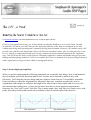
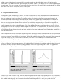
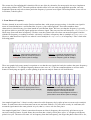
So what happens to the frequencies that are between our frequency gridpoints? Well, we have briefly mentioned the
effect of "smearing", which means that they will make the largest contribution in magnitude to the bin that is closest in
frequency, but they will have some of the energy "smeared" across the neighbouring bins as well. The graph below
depicts how our magnitude spectrum will look like in this case.
Graph 2.1: Magnitude spectrum of a
sinusoid whose frequency is exactly
centered on a bin frequency. Horizontal
axis is bin number, vertical axis is
magnitude in log units
Graph 2.2: Magnitude spectrum of a
sinusoid whose frequency is halfway
between two bins. Horizontal axis is bin
number, vertical axis is magnitude in log
units
As we can see from the above graph, when the measured signal coincides with a bin frequency it will only contribute to
that bin. If it is not exactly centered on one of the bin frequencies, its magnitude will get smeared over the neighbouring
bins which is why the graph in 2.2. has such a broad basis while the graph in 2.1 shows just a peak at bin 50.
The reason why I'm outlining this is that this effect is one of the key obstacles for most people who try to implement
pitch scaling with the STFT. The main problem with this effect isn't even really the magnitude spectrum, since the
magnitude spectrum only tells us that a particular frequency is present in our signal. The main problem, as we will see
in a minute, is the bin phase.
3. From Phase to Frequency
We have learned in our article on the Fourier transform that - with proper post-processing - it describes our signal in
terms of sinusoids that have a well defined bin frequency, phase and magnitude. These three numbers alone
characterize a sinusoid at any given time instant in our transform frame. We have seen that the frequency is given by
the grid on which we probe the signal against our reference signal. Thus, any two bins will always be sampleRate/N
Hertz away from each other in frequency. We have seen above that in the case where our measured signal coincides
with the bin frequency everything is smooth - obviously it will have a frequency that is a multiple of sampleRate/N.
However, what should we expect to see when it is not a multiple of sampleRate/N in frequency? Take a look at the
following graph:
Graph 3.1: Let this be the waveform of a
measured signal with a frequency that is
exactly that of a bin (click to enlarge)
Graph 3.2: Let this be the waveform of a
measured signal with a frequency that is
not on a bin frequency (click to enlarge)
These two graphs look pretty normal, except that we see that the two signals obviously do not have the same frequency the one depicted in 3.2 is of higher frequency than our sine wave in 3.1. We have announced that we will use short
frames for analyzing our signals, so after splitting it up into our analysis frames it will look like this:
Graph 3.3: Our signal of 3.1 now split into 7
frames. Each frame will be passed to our
transform and be analyzed (click to enlarge)
Graph 3.4: Our signal of 3.2 now split into 7
frames. Each frame will be passed to our
transform and be analyzed. We see that
while the signal in 3.3 nicely fits into the
frames, the second signal appears to have a
phase shift in each window (click to enlarge).
Our sampled signal from 3.1 that is exactly centered on a bin frequency nicely splits up into seven successive analysis
frames. In each frame, the waveform starts out at zero and ends with zero. To put it more exactly: in each frame, the
measured signal starts at the same point in its cycle, that is, it starts with the same phase.
Our sampled signal from 3.2 that is somewhere between two bins in frequency does not nicely split into our seven
successive analysis frames. In each frame, the waveform has a clearly visible phase offset, ie. it begins at a different
point in its cycle. The more off-center it is in frequency from the bin frequency, the larger this phase offset will be. So,
what we see here is that while signals whose frequency is exactly on a bin frequency have the same phase offset in each
frame, the phase of signals that have a frequency between two bin frequencies will have an offset that is different with
each frame. So, we can deduce that a phase offset between two frames denotes a deviation in frequency from our bin
frequencies.
In other words: if we measure our k-th sinusoid with its bin magnitude, frequency and phase, its magnitude will denote
to what extent that particular frequency is present in our signal, the frequency will take on its bin frequency and the
phase will change according to its deviation from that bin frequency. Clearly, since we now know that a change in
phase with each frame means a deviation in frequency from the bin frequency, we could as well use the phase offset to
calculate the sinusoids' true frequency. So, we can reduce the three numbers we get back from our post-processed
analysis for each sinusoid, namely bin magnitude, bin frequency and bin phase to just magnitude and true frequency3.
Mathematically, computing the change of a parameter is known as differentiation (which means "taking the difference",
or, in the case of a function, computing the functions' derivative), since we need to compute the difference between the
current parameter value and the last parameter value, ie. how much it has changed since our last measurement. In our
specific case, this parameter is the bin phase. Thus, we can say that the k-th partials' deviation in frequency from its bin
frequency is directly proportional to the derivative of the bin phase. We will use this knowledge later to compute the
true frequency for that partial.
4. About The Choice of Stride
As if this wasn't enough to consider, we also have to worry about another problem. Simply splitting the signal into
successive, non-overlapping frames like we have used in our above illustration does not suffice. For several reasons,
most importantly the windowing4 that needs to be done to reduce the "smearing" of the bin magnitudes, and in order to
be able to uniquely discriminate the bin phase derivative without ambiguity, we need to use overlapping frames. The
typical overlap factor is at least 4, ie. two adjacent windows overlap by at least 75%. Fortunately, the significance of the
frame overlap on bin phase and its derivative is easy to calculate and can be subtracted out before we compute the true
bin frequency. We will see how this is done in the source code example below. Actually, it is pretty unspectacular since
we simply calculate how far our bin phase derivative is expected to advance for a given overlap and then subtract this
offset from our phase difference prior to computing the k-th partials' true frequency.
The other, more important thing we need to consider which is associated with this, however, is that the choice of the
overlap affects the way our true partial frequencies are discriminated. If we have frames that are overlapping to a great
extent, the range in which the true frequency of each of the sinusoids can vary will be larger than if we choose a smaller
overlap.
To see why this is the case, let us first consider how we actually measure the bin phase. As we can see from our source
code example, we use the arc tangent of the quotient of sine and cosine part (in the source code example, they are
referred to as imaginary (im) and real (re) part of each bin for mathematical terminology reasons). The sign of the sine
and cosine parts denote the quadrant in which the phase angle is measured. Using this knowledge we can assume that
the bin phase will always be between -π and +π at any time, since this is the range of our atan2() functions' return
value. Therefore, the increase in phase between any two adjacent frames has an upper limit, with a negative angle
difference denoting a negative deviation from the bin frequency and a positive angle difference denoting a positive
deviation in frequency from the bin frequency. To make sure the phase difference value is centered around 0 (ie.
measured as an absolute value against the origin, that is, always in the range ±π which we need in order to measure the
frequency deviation) we wrap the phase difference back into our ±π interval. This is necessary since the phase offset we
subtract out to make up for the overlap may cause our phase difference to be outside that interval.
Now, in the simple case that any two adjacent frames will not overlap and we know we have an interval of ±π to denote
the deviation in frequency of one partial from our bin frequency, we would only be able to discriminate a frequency
deviation that is ±0.5 bins since this is the maximum advance in phase between two frames we can unambiguously
discriminate in this case. When the frequency of our measured signal crosses the boundary between the two adjacent
STFT bins, the phase difference will wrap back to the beginning of our interval and that partials' frequency will be far
away from the actual frequency of our input sinusoid.
Pass #1: 2411.718750 Hz (bin 112.0):
Bin number
Bin frequency
[Hz]
Bin
magnitude
Bin phase difference
Estimated true frequency [Hz]
110
2368.652344
0.000000
-0.403069
2367.270980
111
2390.185547
0.500000
0.000000
2390.185547
112
2411.718750
1.000000
0.000000
2411.718750
113
2433.251953
0.500000
0.000000
2433.251953
114
2454.785156
0.000000
0.112989
2455.172383
Pass #2: 2416.025391 Hz (bin 112.2):
Bin number
Bin frequency
[Hz]
Bin
magnitude
Bin phase difference
Estimated true frequency [Hz]
110
2368.652344
0.022147
1.256637
2372.958983
111
2390.185547
0.354352
1.256637
2394.492187
112
2411.718750
0.974468
1.256637
2416.025391
113
2433.251953
0.649645
1.256637
2437.558594
114
2454.785156
0.046403
1.256637
2459.091797
Pass #3: 2422.270020 Hz (bin 112.49):
Bin number
Bin frequency
[Hz]
Bin
magnitude
Bin phase difference
Estimated true frequency [Hz]
110
2368.652344
0.024571
3.078761
2379.203614
111
2390.185547
0.175006
3.078761
2400.736816
112
2411.718750
0.854443
3.078761
2422.270020
113
2433.251953
0.843126
3.078761
2443.803223
114
2454.785156
0.164594
3.078761
2465.336426
We can see that when we start out at exactly the frequency of bin 112 as shown in the table of pass #1, the true
frequencies for all channels that are significant (ie. have nonzero magnitude) are correctly centered on their bin
frequencies as is to be expected considering we use a frequency that is a perfect fit. The 0.5 value for the magnitude of
bin 111 and 113 is due to the windowing we use. When we increase the frequency of our measured signal in pass #2 to
be 20% away from the 112th bin's frequency, we see that bin 112 correctly tracks our signal, while the bin above,
towards which the frequency moves, goes even farther away from the correct frequency although its magnitude
increases. This is because it wraps back in its interval and actually goes into the opposite direction! This gets even more
evident in pass #3 which shows that the 113th bin (which should actually be closer to the true frequency of our
measured signal now according to its magnitude) goes even more into the wrong direction.
Pass #4: 2422.485352 Hz (bin 112.5):
Bin number
Bin frequency
[Hz]
Bin
magnitude
Bin phase difference
Estimated true frequency [Hz]
110
2368.652344
0.024252
-3.141593
2357.885742
111
2390.185547
0.169765
-3.141593
2379.418945
112
2411.718750
0.848826
-3.141593
2400.952148
113
2433.251953
0.848826
-3.141593
2422.485352
114
2454.785156
0.169765
-3.141593
2444.018555
In pass #4, the frequency of our measured signal is now halfway between two bins, namely between bin 112 and 113.
We can see this from the bin magnitude, which reflects this fact by having an identical value for these two bins. Now
bin 113 takes on the correct frequency, while bin 112 wraps back to the beginning of its interval (from 3.079 ♠ 3.1415
[+π] to -3.1415 [-π]).
For comparison, here's how the numbers look like when we use an overlap of 75%:
Pass #5: 2422.485352 Hz (bin 112.5), 4x overlap:
Bin number
Bin frequency
[Hz]
Bin
magnitude
Bin phase difference
Estimated true frequency [Hz]
110
2368.652344
0.024252
-2.356196
2336.352516
111
2390.185547
0.169765
2.356194
2422.485348
112
2411.718750
0.848826
0.785398
2422.485352
113
2433.251953
0.848826
-0.785398
2422.485351
114
2454.785156
0.169765
-2.356194
2422.485355
115
2476.318359
0.024252
2.356196
2508.618186
When we want to alter our signal (which we need to do in order to achieve the pitch scaling effect), we see that with no
overlap we easily run into the scenario (depicted in pass #4 above) where on resynthesis we have two sinusoids of equal
amplitude but actually one bin apart in frequency. In our case, this would amount to a difference in frequency of about
21.5 Hz. Thus, when putting our signal back together we would have two sinusoids that are apparently 21.5 Hz apart
where we had one single sinusoid as input. It is not surprising that the synthesized signal will not sound very much like
the original in this case. Clearly, when we just resynthesize the signal without pitch scaling we can expect that these
effects will cancel out. However, this no longer holds in the case when we alter our signal by scaling the partial
frequencies - we would expect that this will introduce an audible error in our signal since the wrapping will now happen
at a different rate.
When we look at pass #5 which uses a 4x overlap (ie. 75%), we see that all adjacent sinusoids down to a bin magnitude
of 0.17 (approx. -15 dB) have about the same frequency, the error can be considered negligible. The next sinusoid that
does not have the correct frequency is approximately -32dB down, which is much better than in the case where we used
no overlap. Thus, we would expect this to sound considerably better. As you can easily verify with the code below, this
is indeed the case.
Summarizing the above, we see that choosing a larger overlap, which is actually oversampling our STFT in time,
increases our ability to estimate the true frequency of our measured sinusoid signal by making the range in which each
sinusoid can deviate from its bin frequency larger: a range of ±1/2 period (±π) has a different meaning when we space
our frames more closely, as the same phase difference for 2x and 4x overlap means twice as high a frequency deviation
in the 4x case than in the 2x case. Thus, the closer we space our frames, ie. the more they overlap, the better we will be
able to determine our true sinusoid frequencies in our measured signal. Of course, the computational cost will also
increase, since we need to perform twice as many STFTs when we increase our overlap from 50% to 75%.
As a consequence for its practical implementation we now see why we need an overlap that is sufficiently large: if we
have a measured signal whose frequency is between two bins, we will have two bins with large magnitude. However,
since the true frequency is somewhere between the two bins and each bin can only deviate by a fixed amount depending
on the overlap, we may have two prominent sinusoids that play at two different, yet close frequencies. Even worse, if
the true frequency of the sinusoid is between the two bins k and k+1 like in our example shown in pass #4, the
frequency of the sinusoid k will move farther away from the true frequency since its phase difference will - trying to
lock on the frequency of the input sinusoid - wrap into the opposite branch. This will produce audible beating in our
resynthesized sound and thus scramble our result. A 75% overlap remedies this situation: adjacent sinusoids down to an
acceptable magnitude are now able to always lock on the true frequency without wrapping - they have become more
"flexible" in frequency which will yield a considerably better sonic quality. As a result, the beating is almost
completely gone.
5. Scaling the Pitch
Once we have mastered the difficulties of calculating the true partial frequencies for our bins, scaling the pitch is
comparably easy. Let's look at what we now have gained after calculating the partials' true frequencies: first, we have
an array of numbers that holds our magnitude values. When we scale the pitch to become sharp, we expect our
magnitude array to expand by our pitch scale factor towards the upper frequency end. Likewise, when we scale our
pitch to become flat, we expect our magnitude spectrum to contract towards the low frequency end. Obviously, the
actual magnitude values stored in the array elements should not change, as a pure sine of -2dB at 1000 Hz is expected
to become a pure sine of -2dB at 500 Hz after a 0.5 x pitch scaling. Second, we also have an array that holds the true
frequencies of our partial sinusoids. Like with the magnitude spectrum, we would also expect our frequency spectrum
to expand or contract according to the scale factor. However, unlike the magnitude values, the values stored in our
frequency array denote the true frequencies of our partials. Thus we would expect them to change according to the pitch
scale factor as well.
We might think that we could simply use an interpolation (upsampling) or decimation (downsampling) process to
achieve the contraction or expansion of the data sets in our magnitude and frequency arrays. But which type of
interpolation would be appropriate. Linear? Polynomial? Bandlimited? Let's think about it for a moment: we have seen
that the bins in the vicinity of the frequency of our sampled sinusoid input signal are locked to this frequency, so the
frequency spectrum will have the same frequency value for several neighbouring bins whenever there is a sinusoid in
our input signal near that frequency. Thus, when we scale the pitch up or down, any complicated way of interpolating
our frequency array might actually be a waste of time as any two adjacent bins will have approximately the same
frequency value anyway. This justifies the use of a zero order hold interpolation to scale our frequency and magnitude
spectrum.
As a trick to improve the output slightly when we lower the pitch and it happens that more than one of our analysis bins
fall on one synthesis bin, we first check if the bin already holds a magnitude value that is larger than the one we would
put into it. If so, we just leave it alone since we assume the largest magnitude will be the most prominent frequency on
resynthesis. If the stored bin magnitude however is lower than our new candidate, it gets replaced. This is an efficient
implementation to ensure the perceptually most relevant partials are preferred. Of course, simply putting the
frequencies in their new bin locations does not suffice, we need to scale their frequency values as well in order to make
the new bin adopt the correct frequency.
Now we also see why pitch scaling using this procedure automatically includes anti-aliasing: we simply do not compute
bins that are above our Nyquist frequency by stopping at fftFrameSize2. This does not even need an additional
processing step.
6. Back to where we came from...
To obtain our output signal, we need to undo all steps that we took to get our magnitude and frequency spectra. For
converting from our magnitude and frequency representation back to bin magnitude, bin frequency and bin phase we
follow the same path back that brought us here. Since the sine and cosine parts of the STFT are periodic and defined for
all time and not just in a certain interval, we need not care for phase rewrapping explicitely - this is done by the basis
functions automatically at no extra cost. After taking the inverse Fourier transform (for which we use the routine
smsFft() from our DFT à Pied article) we string our overlapping frames together at the same choice of stride to get
back our pitch scaled signal.
7. The Code
So how do we actually implement it in software? First, we obtain our current STFT frame from a FIFO queue. This is
required since we don't want to be forced to use a particular input buffer size - this way we can process all data
independent of the FFT frame size we use for the actual pitch scaling. The data is windowed and [re, im] interleaved
into the gFFTworksp array where it gets transformed by the Fast Fourier Transform algorithm smsFft(). This FFT
algorithm isn't particularly efficient, it's just there to demonstrate how to use the routine and to make it compile without
modification. You might replace it by your flavor of the FFT later. smsFft() can be found at the end of our DFT à
Pied article.
Now we're equipped with the complex output for the positive and negative frequencies of our DFT bins. Note that we
only need the positive frequencies as our original signal was purely real. We convert them to magnitude and phase by
rectangular to polar conversion and obtain the instantaneous bin frequency from the phase difference between two
adjacent STFT frames. From that we deduce and compensate for the expected, frequency dependent advance in phase
between two adjacent frames and obtain the true partial frequency. After doing the actual pitch scaling process
described in (6) above, we undo our frequency domain wizardry and then transform to get back to our newly created
time domain sequence. After de-interlacing the [re, im] array, windowing and rescaling we put the data into the output
queue to make sure we have as much output data as we have input data. The global I/O delay is inFifoLatency
samples (which means that the start of your output will contain that many samples of of silence!) - this has to be taken
into account when we write the data out to a file.
Worth noting: The routine smsPitchScale() uses static variables to store intermediate results. This is rather
inelegant and should be replaced by appropriately allocated and initialized memory instead. Note also on routine
parameters: The routine smsPitchScale() takes a pitchScale factor value which is between 0.5 (one octave down)
and 2. (one octave up). A value of exactly 1 does not change the pitch. If you need a wider pitch scale range you need
to tweak the code a bit. numSampsToProcess tells the routine how many samples in indata[0...
numSampsToProcess-1] should be pitch scaled and moved to outdata[0 ... numSampsToProcess-1].
This can be any number of samples. The two buffers can be identical (ie. it can process the data in-place).
fftFrameSize defines the FFT frame size used for the processing. Typical values are 1024, 2048 and 4096. For a
sample rate of 44.1kHz, a value of 1024 is generally fine for speech, while a value of 2048 works well with music. It
may be any value <= MAX_FFT_FRAME_LENGTH but it MUST be a power of 2 unless you use an FFT that can deal
with other frame sizes as well.
8. Conclusion
In this article we discussed a way to use the STFT for changing the perceived pitch of an audio signal by representing it
as a sum of sinusoids and scaling the frequency of these sinusoids. We have detailed the steps necessary to convert the
raw output of a discrete Fourier transform to a musically meaningful representation by making the STFT partials lock
and track the actual harmonics in our input signal to the extent permitted by this 'generic' representation. We have then
used this data to alter the pitch of the underlying signal. C source code for implementing the above process in a blackbox type routine that takes and returns any number of sample values as provided by the calling application is given in
Appendix A below, subject to the terms set forth in the WOL Wide Open software License.
Have fun!
Stephan M. Sprenger, The DSP Dimension
November 1999
1In the literature, one frequently encounters the process of changing the pitch of a signal without changing its length under the name 'Pitch Shifting'. The
author believes that this term is inappropriate. In psychoacoustics where the concept of pitch actually comes from, 'pitch' refers to the perceived quality
of a sound known as its 'apparent fundamental frequency'. In the physical world, this quality can either be the 'real' (actual) fundamental frequency of the
sound (as can be observed in the case of a pure sine wave), but it can also be a quality determined by the most frequently occurring relative spacing
between the harmonics in a sound. Our auditory system is capable of perceiving 'pitch' based on the relative spacing of the sounds' harmonics even if
the actual fundamental frequency is not present in the sound. In a harmonic sound - actually the only sensible context in which pitch has a meaning - all
'harmonics' or 'overtones' are an integer multiple of a fundamental frequency when we assume a linear frequency scale (ie. double scale index = double
frequency). This scale is also what we get when we obtain the magnitude and phase spectrum from the STFT, and is actually the only one that explains
the concept of harmonic sounds in a satisfactory manner ("integer multiples of the fundamental frequency"). When we're doing pitch scaling, it is the
spacing of the harmonics that is scaled when the pitch is scaled, thus the author prefers calling this process 'Pitch Scaling'. The process changes the
distance between any two harmonics by multiplying their frequencies with a scaling factor. Also, we're actually performing the operation on a linear scale
(our STFT output), thus there is no 'shifting' involved at any stage. True 'Pitch Shifting' in this manner would actually rather mean adding an offset to the
interval between the harmonics, which is not suited for the task at hand as it will distort the harmonic relationship of the signals' overtones.
2The term "frequency domain" is a common yet somewhat imprecise nickname widely used for the raw output of the Fourier transform. We will use this
term in this article only in conjunction with the notion of frequency as introduced by the pitch scaling process implemented below, where it denotes an
array of numbers containing the true frequencies of our partials derived by properly post-processing the Fourier transform output.
3this steps assumes an initial condition for the bin phases which the computation of the sinusoids' true frequency is based on. In our discussion we will
always assume the initial phases are set to zero as the phase difference of the second to the first frame will make successive frequency estimates take
on appropriate phase values.
4windowing is a process where the signal is faded in and out during one STFT frame in a particular manner. This suppresses the energy that gets
smeared over adjacent bins to some extent, since an in such a way tapered signal has less frequencies generated by the discontinuity at the frame
boundaries. The interested reader is referred to Chris Bores' online course for a detailed introductory explanation of windowing.
Appendix A: File "smsPitchScale.cp":
[Download PC]
[Download
Mac]
[Download
Unix]
/****************************************************************************
*
* NAME: smsPitchScale.cp
* VERSION: 1.01
* HOME URL: http://www.dspdimension.com
* KNOWN BUGS: none
*
* SYNOPSIS: Routine for doing pitch scaling while maintaining
* duration using the Short Time Fourier Transform.
*
* DESCRIPTION: The routine takes a pitchScale factor value which is between
0.5
* (one octave down) and 2. (one octave up). A value of exactly 1 does not
change
* the pitch. numSampsToProcess tells the routine how many samples in
indata[0...
* numSampsToProcess-1] should be pitch scaled and moved to outdata[0 ...
* numSampsToProcess-1]. The two buffers can be identical (ie. it can process
the
* data in-place). fftFrameSize defines the FFT frame size used for the
* processing. Typical values are 1024, 2048 and 4096. It may be any value <=
* MAX_FFT_FRAME_LENGTH but it MUST be a power of 2. osamp is the STFT
* oversampling factor which also determines the overlap between adjacent STFT
* frames. It should at least be 4 for moderate scaling ratios. A value of 32
is
* recommended for best quality. sampleRate takes the sample rate for the
signal
* in unit Hz, ie. 44100 for 44.1 kHz audio. The data passed to the routine in
* indata[] should be in the range [-1.0, 1.0), which is also the output range
* for the data.
*
* COPYRIGHT 1999 Stephan M. Sprenger <[email protected]>
*
*
The Wide Open License (WOL)
*
* Permission to use, copy, modify, distribute and sell this software and its
* documentation for any purpose is hereby granted without fee, provided that
* the above copyright notice and this license appear in all source copies.
* THIS SOFTWARE IS PROVIDED "AS IS" WITHOUT EXPRESS OR IMPLIED WARRANTY OF
* ANY KIND. See http://www.dspguru.com/wol.htm for more information.
*
*****************************************************************************/
#include <string.h>
#include <math.h>
#define M_PI 3.14159265358979323846
#define MAX_FRAME_LENGTH 8192
void smsPitchScale(float pitchScale, long numSampsToProcess, long
fftFrameSize, long osamp, float sampleRate, float *indata, float *outdata)
{
static float gInFIFO[MAX_FRAME_LENGTH];
static float gOutFIFO[MAX_FRAME_LENGTH];
static float gFFTworksp[2*MAX_FRAME_LENGTH];
static float gLastPhase[MAX_FRAME_LENGTH/2];
static float gSumPhase[MAX_FRAME_LENGTH/2];
static float gOutputAccum[2*MAX_FRAME_LENGTH];
static float gAnaFreq[MAX_FRAME_LENGTH];
static float gAnaMagn[MAX_FRAME_LENGTH];
static float gSynFreq[MAX_FRAME_LENGTH];
static float gSynMagn[MAX_FRAME_LENGTH];
static long gRover = false, gInit = false;
double magn, phase, tmp, window, real, imag;
double freqPerBin, expct, fadeZoneLen, fract;
long i,k, qpd, index, inFifoLatency, stepSize, fftFrameSize2;
/* set up some handy variables */
fadeZoneLen = fftFrameSize/2;
fftFrameSize2 = fftFrameSize/2;
stepSize = fftFrameSize/osamp;
freqPerBin = sampleRate/(double)fftFrameSize;
expct = 2.*M_PI*(double)stepSize/(double)fftFrameSize;
inFifoLatency = fftFrameSize-stepSize;
if (gRover == false) gRover = inFifoLatency;
/* initialize our static arrays */
if (gInit == false) {
memset(gInFIFO, 0, MAX_FRAME_LENGTH*sizeof(float));
memset(gOutFIFO, 0, MAX_FRAME_LENGTH*sizeof(float));
memset(gFFTworksp, 0, 2*MAX_FRAME_LENGTH*sizeof(float));
memset(gLastPhase, 0, MAX_FRAME_LENGTH*sizeof(float)/2);
memset(gSumPhase, 0, MAX_FRAME_LENGTH*sizeof(float)/2);
memset(gOutputAccum, 0, 2*MAX_FRAME_LENGTH*sizeof(float));
memset(gAnaFreq, 0, MAX_FRAME_LENGTH*sizeof(float));
memset(gAnaMagn, 0, MAX_FRAME_LENGTH*sizeof(float));
gInit = true;
}
/* main processing loop */
for (i = 0; i < numSampsToProcess; i++){
/* As long as we have not yet collected enough data just read in */
gInFIFO[gRover] = indata[i];
outdata[i] = gOutFIFO[gRover-inFifoLatency];
gRover++;
/* now we have enough data for processing */
if (gRover >= fftFrameSize) {
gRover = inFifoLatency;
/* do windowing and re,im interleave */
for (k = 0; k < fftFrameSize;k++) {
window = -.5*cos(2.*M_PI*(double)k/(double)fftFrameSize)+.5;
gFFTworksp[2*k] = gInFIFO[k] * window;
gFFTworksp[2*k+1] = 0.;
}
/* ***************** ANALYSIS ******************* */
/* do transform */
smsFft(gFFTworksp, fftFrameSize, -1);
/* this is the analysis step */
for (k = 0; k <= fftFrameSize2; k++) {
/* de-interlace FFT buffer */
real = gFFTworksp[2*k];
imag = gFFTworksp[2*k+1];
/* compute magnitude and phase */
magn = 2.*sqrt(real*real + imag*imag);
phase = atan2(imag,real);
/* compute phase difference */
tmp = phase - gLastPhase[k];
gLastPhase[k] = phase;
/* subtract expected phase difference */
tmp -= (double)k*expct;
/* map delta phase into +/- Pi interval */
qpd = tmp/M_PI;
if (qpd >= 0) qpd += qpd&1;
else qpd -= qpd&1;
tmp -= M_PI*(double)qpd;
/* get deviation from bin frequency from the +/- Pi interval */
tmp = osamp*tmp/(2.*M_PI);
/* compute the k-th partials' true frequency */
tmp = (double)k*freqPerBin + tmp*freqPerBin;
/* store magnitude and true frequency in analysis arrays */
gAnaMagn[k] = magn;
gAnaFreq[k] = tmp;
}
/* ***************** PROCESSING ******************* */
/* this does the actual pitch scaling */
memset(gSynMagn, 0, fftFrameSize*sizeof(float));
memset(gSynFreq, 0, fftFrameSize*sizeof(float));
for (k = 0; k <= fftFrameSize2; k++) {
index = k/pitchScale;
if (index <= fftFrameSize2) {
/* new bin overrides existing if magnitude is higher */
if (gAnaMagn[index] > gSynMagn[k]) {
gSynMagn[k] = gAnaMagn[index];
gSynFreq[k] = gAnaFreq[index] * pitchScale;
}
/* fill empty bins with nearest neighbour */
if ((gSynFreq[k] == 0.) && (k > 0)) {
gSynFreq[k] = gSynFreq[k-1];
gSynMagn[k] = gSynMagn[k-1];
}
}
}
/* ***************** SYNTHESIS ******************* */
/* this is the synthesis step */
for (k = 0; k <= fftFrameSize2; k++) {
/* get magnitude and true frequency from synthesis arrays */
magn = gSynMagn[k];
tmp = gSynFreq[k];
/* subtract bin mid frequency */
tmp -= (double)k*freqPerBin;
/* get bin deviation from freq deviation */
tmp /= freqPerBin;
/* take osamp into account */
tmp = 2.*M_PI*tmp/osamp;
/* add the overlap phase advance back in */
tmp += (double)k*expct;
/* accumulate delta phase to get bin phase */
gSumPhase[k] += tmp;
phase = gSumPhase[k];
/* get real and imag part and re-interleave */
gFFTworksp[2*k] = magn*cos(phase);
gFFTworksp[2*k+1] = magn*sin(phase);
}
/* zero negative frequencies */
for (k = fftFrameSize+2; k < 2*fftFrameSize; k++) gFFTworksp[k] = 0.;
/* do inverse transform */
smsFft(gFFTworksp, fftFrameSize, 1);
/* do windowing and add to output accumulator */
for(k=0; k < fftFrameSize; k++) {
window = -.5*cos(2.*M_PI*(double)k/(double)fftFrameSize)+.5;
gOutputAccum[k] += 2.*window*gFFTworksp[2*k]/(fftFrameSize2*osamp);
}
for (k = 0; k < stepSize; k++) gOutFIFO[k] = gOutputAccum[k];
/* shift accumulator */
memmove(gOutputAccum, gOutputAccum+stepSize, fftFrameSize*sizeof(float));
/* move input FIFO */
for (k = 0; k < inFifoLatency; k++) gInFIFO[k] = gInFIFO[k+stepSize];
}
}
}
Last change: 29.11.1999, ©1999 S. M. Sprenger, all rights reserved. Content subject to change without notice. Content provided 'as is', see disclaimer.
Graphs made using Algebra Graph, MathPad, sonicWORX and other software. Care has been taken to describe everything as simple yet accurate as
possible. If you find errors, typos and ambiguous descriptions in this article, please notify me and I will correct or further outline them.
Special thanks to Richard Dobson for providing immensely useful suggestions and corrections to my incomplete knowledge of the English language.
*Original article "S.Sprenger: Using The STFT For Time and Pitch Scaling - Analysis, Implementation and Improvement" with code funded by the UCMG
Media Association in grant No. 94030233 as part of the Media Network Associate Training Program (MNATP 3, March 1994). Re-used with permission.
Coming soon...
Read more about the synthesis technology behind the Hartmann <Neuron> synthesizer, and get the inside
track on what it is all about.
Coming up on this web page soon. In the meantime, make sure you check out the official Hartmann
Music web page at http://www.hartmann-music.com
last change: 27.01.2003, ©2003 S. M. Sprenger, all rights reserved. Content subject to change without notice. Content provided 'as is',
see disclaimer.
C Programming - Useful and Fun Stuff
Hi again. This is the page where I collect things that I wrote for debugging and simulation purposes that might be worth sharing. Or
more generally, things I've done that I find particularly funny or useful, which are related to C programming or audio DSP. If you are
in search of a really useful web site on DSP tricks, make sure you visit the comp.dsp folk's DSPguru web site, too.
ASCII Art - Plotting a Waveform On The Console
I often run into the problem of showing people, either personally or on remotely through email or usenet groups, a certain output of a
DSP process. But: some people work on UNIX, others on Windows or on the Mac. Writing code that draws on the screen for each
platform is tedious, and unnerving if you only want to display some basic things like waveforms or spectra at a reasonably coarse
resolution. Also, when posting to usenet news groups, binary attachments are either not permitted or not possible, and are stripped off
the message when it is stored in an archive. Therefore, most people "draw" their waveforms by typing appropriate characters for each
point, which we call "ASCII Art".
smsPlotWave() does exactly that. It draws a discrete signal, stored in a float buffer, via ASCII Art on the screen. It does this at a
fairly coarse resolution, but it does it nicely and is entirely cross platform. Make sure you use a monospace font, though! The
resulting "image" can be copied and pasted into an email, which is very convenient. It is also great for debugging purposes, when you
don't have the time to bother with graphics.
smsPlotWave() only uses stdio commands, which are available on all platforms.
Enjoy!
Listing 1.0: consolePrintWave displays a discrete waveform via ASCII art
#define DISP_STR_MAXLEN
256
bool smsPlotWave(float *data, long rowLength)
//Prints waveform row-wise to the console
//(c) 1999 S.M.Sprenger, made available under the WOL
//Returns false when something wet wrong, true otherwise
//data[] contains the data to be displayed. It is assumed that the
//data values lie between -1.0 and +1.0, please normalize your
//data accordingly
//rowLength is the length of all rows. Usually, this is between 60-80
//characters
{
char printString[DISP_STR_MAXLEN];
long numRows = 21;
if (data == 0)
return false;
if (rowLength > DISP_STR_MAXLEN-3)
return false;
for (long i = 0; i < numRows; i++) {
sprintf(printString, "%3.0d >", -i+numRows/2);
long lastQdata = 0;
for (long j = 0; j < rowLength; j++) {
long qData = (long)((float)(numRows-1)*(.5+.5*data[j])+.5);
if (qData == i) {
if (qData-lastQdata > 0)
sprintf(printString, "%s`", printString);
else if (qData-lastQdata < 0)
sprintf(printString, "%s,", printString);
else sprintf(printString, "%s-", printString);
} else {
if (i == numRows/2) sprintf(printString, "%s-", printString);
else sprintf(printString, "%s ", printString);
}
lastQdata = qData;
}
sprintf(printString, "%s\n", printString);
printf("%s",printString);
}
printf("\n");
return true;
}
last change: 18.08.2002, ©2002 S. M. Sprenger, all rights reserved. Content subject to change without notice. Content provided 'as is', see disclaimer.
On to the
DSPguru Web
Site
Please see the disclaimer
before using the links
provided on this page
My favourite sites
DSPguru
Dave Hales FFT Laboratory (needs Java)
.
Jeffrey Taft's Java Applets for digital filter design (requires IE5)
Amara's Wavelet Resources
Lotsa lotsa Linxx -unorderedHarmony Central
Comp.dsp Frequently Asked Questions (FAQs)
Ludger's Research Page
Technical Reports
Csound.faq.1.02.html
Numerix Home Page
Introduction to Signal Processing
Papers by Eric Scheirer
DSPT Signal Analysis Group
Linear Predictive Coding (LPC)
Subband Coding
Olli Niemitalo's Audio Signal Processing page
The Music DSP Archive
Colors_of_noise_pseudo_FAQ
Directory of /pub/comp.speech/info
Devin McAuley's Home Page
//cnmat.CNMAT.Berkeley.EDU/Rese
Macintosh Music Shareware and Freeware Music Players and Editors
Wavelet Resources
. BrainWave: a multiplatform connectionist simulator
Publications Archive
The MBROLA PROJECT HOMEPAGE
www.ObjektSynth.com: FAQ
Computer Music Journal Home Page
Digital audio experiments by Don Cross
Performance Evaluation and Real-Time Implementations of Subspace, Adaptive, and
DFT Algorithms for Multi-Tone Detection
Mac RLab
FFTW Home Page
SNDAN
computer music programs . macintosh
SoundApp Home Page
Dr. Dobb's Web Site
References on the Hilbert Transform Applications
hilbert2.html
1994.03
The Fibonacci Numbers and the Golden section
Fibonacci Representations of integers
Bryan Holloway's M.S. Thesis
Mostly Wavelet-related
Directory of /pub/som_pak
Amara's Wavelet Page
Khoros Wavelet and Compression Toolbox
MacWavelets Home Page
.
Wavelet Digest Home Page
Wavelet Group Karlsruhe: Software
Wavelet Resources
Wavelets
Mostly about Artificial Neural Networks
Commercial Applications of Neural Networks
Neural Networks Research Centre @ hut.fi
. Neural Network FAQ, part 1 of 7: Introduction
NNSP Home Page
Papers
Misc DSP
Miranda's CMJ Paper
CORDIC Bibliography
DSP Internet Resources
Numerical Recipes in C
Numerical Recipes Public Domain Area
Andraka Consulting Group Home Page
IEEE Signal Processing Society
Optimal Radially Gaussian Kernel TFR
Rice DSP Publications Archive
. Rice University Digital Signal Processing
Signal Processing Information Base (SPIB)
Signal Processing URL Library (SPLIB)
SIPB WWW Server Home Page
SPIB - Signal Processing Information Base
Internet Digital Signal Processing Tools and Embedded Systems Resources
PHOAKS: Resources for comp.dsp
Princeton University Home Page
Stanford University Homepage
TECHNOLOGY AND ENGINEERING SCIENCES
Music-DSP related
Ircam
Cellular Approach for Modeling Room Acoustics
Lemur: A Tool for Timbre Manipulation
Jörgs useful and ugly Homepage
Computer Music and Digital Audio Series
.
Digital Audio Signal Processing
AES Papers
SoundHack User's Manual
the FOURIER page
SHARC Timbre Database Documentation
Hardware DSP stuff
Fast Mathematical Algorithms & Hardware
. Analog Devices
DSP Processor Fundamentals
Programming
Comp.dsp Frequently Asked Questions (FAQs)
Metrowerks WorldWide
.
SGI audio Frequently Asked Questions (FAQ)
The MathWorks Web Site
last change: 21.09.2000, ©1999-2000 S. M. Sprenger, all rights reserved. Content subject to change without notice.
Content provided 'as is', see disclaimer.
NEW: Scroll
down for details
on my past and
present work
Stephan M. Sprenger is with Prosoniq since 1990. Being the actual founder of
Prosoniq, he has led the company through many years of difficult decisions in
the short lived music and audio software market. With the incorporation of
Prosoniq in the UCMG network in 1993, he became senior developer of the
R&D department for media and production at UCMG due to exceptional
achievements. In 1995, Prosoniq GmbH was founded as a separate entity again
and Mr. Sprenger took on his present position as head of R&D. He is currently
employed as Director of Research and Development at Prosoniq headquarters
in Karlsruhe, Germany.
Founded in 1990 as a privately held company, Prosoniq has since grown and
gathered a highly acclaimed position as key technology provider through its
cutting edge audio DSP software products. Prosoniq, a daughter company of
the UCMG Corp. since 1993, licenses audio DSP technology and applications
to many important companies in the music market, such as Emagic, Steinberg,
Ensoniq, BlueSpike and others. Since 1995, Stephan M. Sprenger works as
Director of Research and Developement supervising all development and
implementing a large part of the key technologies used in Prosoniq's products.
. Born in Karlsruhe, Baden, Germany in 1971 his interest in music DSP
applications arose from his prior work as software consultant for a medical data
processing company where he used Artificial Neural Networks for time series
evaluation of medical data. He soon realized that the same technology can be
successfully applied to audio processing and he subsequently developed the
ANN-CASE Artificial Neural Network design tool for SGI computers that
allowed parametrized development of ANN topologies and training methods on
IRIX workstations.
He has since pioneered several novel methods of decomposing and rebuilding
audio signals at very high quality based on new transformation methods and
highly optimized neural network processing. Being the original developer of
Prosoniq's unique and proprietary MCFE audio decomposition engine he has
contributed the basic techniques and important later refinements to implement
new audio algorithms and processing capabilities that can only be found in
Prosoniq's product line. Being the inventor of the MPEX near-lossless time and
pitch scaling, he currently works on projects on auditory scene analysis, nearlossless time and pitch scaling and on the design and implementation of high
speed neural computing and training methods.
Text ©1999 Prosoniq Products Software GmbH, used with permission
Main work (excerpt):
Here is a brief list of what I've been doing over the past 15 years for a living. Don't bother looking for
papers on any of the topics - since I've been mostly involved in commercial research from the very start
there hardly aren't any for reasons of trade secret and other legal concerns, at least none that are available to
the general public.
Music Industry
My main area of work has been in the music industry, although I've been working in other areas as well
(s.b.).
1988-90
●
●
First model-based structural audio morphing software implemented on an Atari ST
Author for various music-related magazines (KEYS magazine in Germany), various articles on
Digital Signal Processing and DIY courses
1990
●
Self-employed, founded Prosoniq Products Software as privately held company who delivered audio
software for the ATARI 1040ST and for various embedded systems based around the Mot. 68k, 56k
and custom DSP chips.
1991-93
●
●
●
Study of Communications Engineering in Karlsruhe
Co-Development of Medical diagnosis software for a client of Nemectron Corp., Germany
Research and specialization on adapted basis transforms and multiresolution signal analysis
1993
●
●
Acquisition of Prosoniq by the UCGM Corporation, Heidelberg, Germany to expand their
mastering/post production dept. and to produce custom tailored DSP software development for their
needs
Extended study and development of processes based on Artificial Neural Networks and number
theoretic transforms
1993-95
●
●
●
●
●
●
●
●
●
●
●
●
●
●
●
●
Software developer and senior software developer at Prosoniq/UCMG, also responsible for
coordination and supervision of the UCMG studios and mastering facilities and processes
Development of an ANN Topology Editor with C Source Code Generator for SGI IRIX 5.2-6.2
Development of a modular DSP compiler that generates C source code from high-level language
scripts
Vinyl cutting simulator for optimization of vinyl cutting process for UCMG
Developed a psychoacoustic loudness maximizer optimzied for vinyl and CD
Sibilancy suppressor based on sibilance recognition technology employing ANNs
Pitch Scaling algorithm based on the fast Fourier transform
Supervised collection of a speech database and its implementation for later use in speech
recognition products
Devised business plan and technology/component assembly for a 56k based standalone postproduction device (development discontinued due to marketing reasons)
Discussed and planned co-development of a AD65xxx based synthesizer with a major company in
the MI business
Devised a novel noise reduction based on adaptive transform technology and ANNs
Co-development of sonicWORX, a state-of-the-art audio editor
Development of numerous plug in modules for sound manipulation within sonicWORX
Developed 1/3 octave band analyzer for audio
Extensive work on multiresolution sinusoidal modelling using enhanced MQ and D+S signal
decomposition/synthesis, extended into non-rectangular and adaptive transform based methods
Prosoniq GmbH was founded with Bernhard Bouché as CEO. Moved office from the UCMG
facilities to the Karlsruhe Technology Centre
1996-1997
●
●
●
●
●
●
●
Development of a real time lapped transform filterbank for speech coding and vocoder products
(later to become part of OrangeVocoder)
Development of a real time LOT resynthesizer (later to become part of Prosoniq's Magenta product)
Extensive modelling of analogue circuitry (later to be used in the products OrangeVocoder and
NorthPole)
Devised novel multiresolution based formant manipulation to allow for natural sounding
monophonic and polyphonic pitch changing (later to be used in Emagic's Logic Audio range of
products)
Developed a set of realtime effects to complement Emagic Logic Audio 3.0
Development of a fast shift invariant wavelet transform for audio coding and analysis
Development of MCFE time scaling based on complex-valued wavelet packet transform
1997-1999
●
●
●
●
●
Developed acoustic 3D scenery modelling software based on a cellular room modelling approach
(later to be implemented into Prosoniqs "Ambisone" product)
Coordinated porting and feature set of Prosoniq's VST products on the Digidesign RTAS platform
Coordinated and planned feature set development and implementation for Hartmann Neuron
Synthesizer
Co-developed "NorthPole" with Frederic Schelling. NorthPole is a 4pole resonant filter for the VST
interface, to date still the most widely distributed free plug in for VST
Developed realtime lead vocal reduction software based on adaptive, model-driven transform
technology, later implemented in Pandora Realtime for sonicWORX
●
●
●
●
●
●
●
Commenced work on forensic voice separation and blind signal separation software for various
clients and institutions, work in progress
Developed new dithering process for requantization based on geometric series to allow for
minimum noise and maximum clarity (later to be used in sonicWORX)
Development of a time scaling technique based on the fractional Fourier transform
Developed time scaling technology for NewMotion GmbH
Developed custom tailored DSP and filtering applications for NewMotion GmbH
Developed time scaling technology for DAVE GmbH
Frequent poster to comp.dsp, also involved in DSP training and education in Karlsruhe, Heidelberg
and Darmstadt
1999-2002
●
●
●
●
●
●
●
●
●
●
Developed specialized custom-tailored sample manipulation tools for YellowTools makers of
sampling CDs, most notably an automatic pitch-synchronous loop finder
Developed method for loop-matching the contents of a sampled sound to allow for smooth loops
within a user-defined area
Developed Prosoniq's MPEX and MPEX2 (multi-channel) near-lossless time scaling technology
which was highly acclaimed by the public and was awarded several prices. Today it is an integral
part of all major music production software packages.
Implemented MPEX technology for watermark recovery for BlueSpike techology
Implemented MPEX Time Scaling technology for Steinberg Nuendo
Implemented MPEX Technology for Prosoniq TimeFactory which was awarded several prices
Implemented MPEX technology for IRCAM/Apple software
Carried out optimization and parallelization of all Prosoniq algorithms on G4 processors (Altivec
technology) and processor specific optimizations for Pentium III processors
Developed a multiresolution realtime resynthesis technology for sound reproduction for up to 56
voice polyphonic realtime sinusoidal resynthesis on a G4 processor
Implemented enhanced phase coherence pvoc for Roni Music, Sweden.
2002-present
●
●
●
●
●
●
●
●
Extensive research into sound modelling and parametrization based on adaptive transforms and
artificial neural networks
Developed real-time polyphonic rendering engine based on structural audio information
Developed analysis library to perform parametrization and model extraction on sampled sounds
Conducted extensive studies on acoustic performances and instrument timbres to gather data for
parametrization training
Developed NAS technology and custom-fitted it to the Hartmann <Neuron> synthesizer
Adapted MPEX2 time scaling technology for use in Steinbergs Cubase SX
Adapted MPEX2 time scaling technology for use in Merging Technology's Pyramix system
Consultation work for several major companies in the MI and other businesses
1990-present
Web Development
●
●
●
Developed a C-based CGI engine (gcc under Suse Linux) for customer support and registration at
Prosoniq
Developed a C-based CGI engine (gcc under Suse Linux) for context evaluating FAQ generation
(incomplete)
Developed a C-based CGI engine (gcc under Suse Linux) for software bug tracking and reporting
(incomplete)
2002-2003
Optics
●
●
●
Developed a wavelet based image decomposition tool to allow for optically pleasing image scaling
and transformation
Developed an image filtering toolbox based on local fractional Fourier transforms to enhance
research data collected by a LCD sensor
Developed real-time vision-aided onset detection and phoneme recognition software to aid in
collecting data for a TTS database
1990-2003
Screen design:
●
●
●
●
●
●
●
●
Prosoniq TimeFactory GUI
Prosoniq Magenta GUI
Prosoniq Roomulator 1.8
Prosoniq VoxCiter 1.8
Prosoniq Dynasone 1.8
Prosoniq Ambisone 1.8
http://www.prosoniq.com Design and Implementation
http://www.dspdimension.com Design and Implementation
last change: 12.01.2003, ©1999-2003 S. M. Sprenger, all rights reserved. Content subject to change without notice. Content provided
'as is', see disclaimer.