1
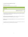
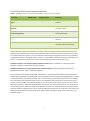
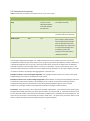
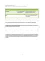
CASE USER MANUAL 2014-06-12 ALGORITHMS, PARAMETER SETTINGS AND EVALUATION MODULE Anna-Maria Kling, Maria Grünewald, Anette Hulth CONTENTS 1. Introduction .................................................................................................................................................... 4 2. Algorithms and parameter settings ................................................................................................................ 5 2.1 Threshold algorithm ...................................................................................................................................... 5 2.2 SaTScan Poisson model ................................................................................................................................. 6 2.3 SaTscan Space-time Permutation model ...................................................................................................... 7 2.4 Farrington algorithm ..................................................................................................................................... 8 2.5 OutbreakP statistic ........................................................................................................................................ 9 3. country of infection and route of transmission ............................................................................................ 10 4. Colour-coding scheme in CASE interface ...................................................................................................... 11 5. Statistical evaluation Module ........................................................................................................................ 13 4.1 Description of wizard .................................................................................................................................. 13 Step 1 – Data source ..................................................................................................................................... 13 Step 2 - Pathogen ......................................................................................................................................... 13 Step 3 – Algorithms, time period, country of infection and route of transmission ................................... 13 Step 3 – Algorithms and time period (continued) ....................................................................................... 14 Step 4 – Overview of test run....................................................................................................................... 14 Step 4 – Overview of test run (Continued) .................................................................................................. 15 Step 5 – Execution ........................................................................................................................................ 15 4.2 Output files from case evaluation module .................................................................................................. 16 4.2.1 Output files from case evaluation module – Farrington algorithm.......................................................... 16 Text file - Farrington algorithm .................................................................................................................... 16 Html file - Farrington algorithm ................................................................................................................... 17 Jpeg file - Farrington algorithm .................................................................................................................... 18 4.2.2 Output files from case evaluation module – Threshold algorithm .......................................................... 18 Text file - Threshold algorithm ..................................................................................................................... 18 Html file - Threshold algorithm .................................................................................................................... 19 2 Jpeg file- Threshold algorithm...................................................................................................................... 19 4.2.3 Output files from case evaluation module – SatScan Space time algorithm ........................................... 20 Text file- SatScan Space time algorithm ...................................................................................................... 20 Html file - SatScan Space time algorithm .................................................................................................... 21 Jpeg file - SatScan Space time algorithm ..................................................................................................... 21 4.2.4 Output files from case evaluation module – SatScan Poisson model ...................................................... 22 Text file- SatScan Poisson model ................................................................................................................. 22 Html file - SatScan Poisson model................................................................................................................ 22 Jpeg file - SatScan Poisson model ................................................................................................................ 23 Text file- Outbreak P..................................................................................................................................... 24 Html file - Outbreak P ................................................................................................................................... 25 Jpeg file – Outbreak P ................................................................................................................................... 25 References ............................................................................................................................................................ 26 3 1. INTRODUCTION CASE (Computer Assisted Search for Epidemics) is a platform for computer supported outbreak detection, implemented at the Public Health Agency of Sweden. This manual is aimed to describe the practical usage of the CASE system, with focus on the choice of algorithms and their parameter values. The manual describes the algorithms as implemented in CASE. The main function of CASE is to warn for potential outbreaks. In some cases, the system might be able to detect outbreaks earlier than human experts. Additionally, it might detect certain outbreaks that human experts would have overlooked. However, the system does not aim to replace human experts (hence the prefix “computer assisted”); it should rather be considered a complement to daily surveillance activities. To a smaller extent, the system can also aid less experienced epidemiologists in identifying outbreaks. Based on case information, such as diagnosis and date, different statistical algorithms for detecting outbreaks can be applied, both on pathogen level and subtype level. The parameter settings for the algorithms can be configured independently for each diagnosis. Five different statistical algorithms are currently implemented in CASE for detection of potential outbreaks. The choice of algorithm for a specific pathogen depends on the distribution of the pathogen and how an outbreak is defined. More than one algorithm can be applied to the same pathogen. Algorithms and parameters are chosen in a graphical user interface by the system administrator. If an outbreak signal is detected an email notification is sent to the persons listed as receivers for that particular pathogen. There may be both outbreaks not detected (false negatives) and a signal when there is no outbreak (false positives). CASE is available as open source software, licensed under GNU General Public License Version 3. By making the code open source, we wish to encourage others to contribute to the future development of computer supported outbreak detection systems, and in particular to the development of the CASE framework. A technical manual for installation of the system is included when downloading the system. The CASE platform has previously been described by Cakici et al (2010) and a user evaluation is presented in Kling et al (2012). 4 2. ALGORITHMS AND PARAMETER SETTINGS 2.1 THRESHOLD ALGORITHM TABELL 1 PARAMETERS FOR THRESHOLD ALGORITHM TO BE SET IN THE CASE INTERFACE Parameter Default value Allowed values Comment Threshold value (number of cases) 5 Integers ≥ 0 Signal is given when threshold is exceeded Detection window (days) 7 Integers ≥ 1 Number of cases is an absolute value so threshold and detection window have to be decided in relation to each other The threshold algorithm, developed by the CASE group, generates a signal when the number of cases exceeds a manually set threshold for a specified time period. The threshold algorithm in CASE is used for surveillance of pathogen data aggregated on a national level. Examples of when to use the threshold algorithm: A signal for a potential outbreak should be generated due to a specific threshold value and time period. Can be useful for rare pathogens. Examples of when not to use the threshold algorithm: When the value of the threshold and the time period is difficult to decide. Two parameters can be altered by the CASE administrator in the interface of the CASE system (see table 1): the threshold value (number of cases) and detection window (number of days). 5 2.2 SATSCAN POISSON MODEL TABELL 2 PARAMETERS FOR SATSCAN DISCRETE POISSON MODEL TO BE SET IN THE CASE INTERFACE Parameter Default value Allowed values Comment Detection window (days) 180 Integers ≥ 90 A large value gives less random variation Population at risk (percent) 50 0<Value<50 A high value allows for both small and large clusters Aggregated days 7 Integers > 0 A value of 7 adjusts for weekly variation Alpha value 0.05 0<Value<1 A large value gives higher sensitivity and lower specificity SaTScan discrete Poison model (Kulldorff, 1997) is used to investigate spatial clustering of cases during a specified period, using a discrete Poisson model, taking population density at different locations into account. Clusters are not restricted to regional boundaries. The algorithm gives a signal when data differ from what is expected in a statistically significant way. Examples of when to use the SatScan discrete Poisson model: Data are available on a sub-national level. The pathogen incidence is similar at different locations when there is no current outbreak. Outbreaks are likely to be spatially clustered. Examples of when not to use the SatScan discrete Poisson model: The pathogen incidence varies with demographic factors, such as age distribution; so that there is a constant spatial clustering (would result in many false positives signals). Routines for detecting and reporting pathogen vary between locations (would result in many false positives signals). Outbreaks are spread out geographically (would result in many false negative signals). Four parameters can be altered by the CASE administrator in the interface of the CASE system: the detection window (days), population at risk (percent), aggregated days, and the p-value (see table 2). The detection window, set as number of days, specifies the time period to be included in the computation of the expected number of cases. The population at risk specifies the maximum size of the clusters; a setting of 50% means that the algorithm will scan for very small clusters up to clusters that include 50% of the population. The p-value is set based on how sensitive the analysis needs to be. The parameter aggregated days is used to adjust for cyclic temporal trends. 6 2.3 SATSCAN SPACE-TIME PERMUTATION MODEL TABELL 3 : PARAMETERS FOR SPACE-TIME PERMUTATION MODEL TO BE SET IN THE CASE INTERFACE Parameter Default value Allowed values Comment Detection window (days) 180 Integers ≥ 90 A large value gives less random variation Population at risk (percent) 50 0<Value<50 A high value allows for both small and large clusters Maximum temporal cluster size (percent) 50 0<Value<50 A high value allows for both short and long outbreaks Aggregated days 7 Integers > 0 A value of 7 adjusts for weekly variation Alpha value 0.05 0<Value<1 A large value gives higher sensitivity and lower specificity SaTScan Space-time algorithm (Kulldorff et al, 2005) is used to investigate spatial and temporal clustering of cases during a specified period, using a discrete Poisson model. If incidence increases everywhere, or an area has a permanent high incidence, it is not considered an outbreak by the algorithm. Clusters are not restricted to regional boundaries. The algorithm gives a signal if a cluster differs from what is expected in both time and space, in a statistically significant way, and if it is still ongoing during any of the last seven days. Examples of when to use the Space-time Permutation model: Data are available on a sub-national level. Pathogen outbreaks are likely to be spatially clustered. Examples of when not to use the Space-time Permutation model: Pathogen outbreaks are spread out geographically (would result in many false negatives). Five parameters can be altered by the CASE administrator in the interface of the CASE system: the detection window (days), population at risk (percent), maximum temporal cluster size (percent), aggregated days, and the p-value (see table 3). The detection window, set as number of days, specifies the time period to be included in the computation of the expected number of cases. The population at risk specifies the maximum size of the clusters; a setting of 50% means that the algorithm will scan for very small clusters up to clusters that include 50% of the population. Maximum temporal cluster size specifies the maximum time period of an outbreak, set as a percentage of the detection window. If the detection window is set to 180 days and max temporal cluster size is set to 50%, the algorithm will scan for ongoing outbreaks lasting from 1 day to 90 days. The p-value is set based on how sensitive the analysis needs to be. The parameter aggregated days is used to adjust for cyclic temporal trends. 7 2.4 FARRINGTON ALGORITHM TABELL 4 PARAMETERS FOR FARRINGTON ALGORITHM TO BE SET IN THE CASE INTERFACE Parameter Default value Allowed values Comment Detection window (start date) 2003-01-01 Dates that that ensures at least 1460 days between start date and date for detection. A long detection window gives less random variation Alpha value 0.01 0<Value<1 A large value gives higher sensitivity and lower specificity Weeks in plot 100 >10 Number of weeks presented in plot. Analysis is performed for each week presented. Analysis relies on data previous to the week analyzed. This means that an early first week (high value of “Weeks in plot”) also requires an early start date in “Detection window”. The Farrington algorithm (Farrington et al, 1996) compares the current number of cases to a threshold computed from historical data in the previous years. A signal is given when data differ from what is expected in a statistically significant way, for at least one of the last two weeks. A week in Farrington starts on Mondays and ends on Sundays. Since the CASE system is running on a daily basis, a signal is more likely to occur in the end of the week because the number of cases are added up during the week. The Farrington algorithm in CASE is used for surveillance of pathogen data aggregated on a national level. Examples of when to use the Farrington algorithm: The pathogen incidence varies over seasons, but is quite stable between years. Data are available from several years. Examples of when not to use the Farrington algorithm: Historical data are missing for the pathogen (the result would show a large random variation). The pathogen has an incidence or frequency of reporting that has changed over the past years (would result in many false positives/negatives signals). There are large fluctuations in pathogen incidence not explained by calendar time (large random variation). Parameters: Three parameters can be altered by the CASE administrator in the interface of the CASE system: the detection window (start date), the alpha value and weeks in plot (see table 4). The detection window is set by start date and specifies which time period should be included in the computation of the threshold limit. The alpha value is set based on how sensitive the analysis needs to be. The value of the parameter weeks in plot sets the number of weeks in the plot produced by the Farrington algorithm. 8 2.5 OUTBREAKP STATISTIC TABELL 5 PARAMETERS FOR OUTBREAK P STATISTIC TO BE SET IN THE CASE INTERFACE Parameter Default value Allowed values Comment Aggregated days (start date) 2007-01-01 Maximum value equals the number of days for which data exist A long detection period gives less random variation given that the distribution is stable over time Alarm statistic level 1000 Integers ≥to 0 Depends on pathogen incidence. To set this value a simulation procedure can be helpful. The Outbreak P statistic (Frisén et al, 2009) is here used to investigate, on a national level, if the number of cases in a week is increasing more than expected, which implies a potential outbreak. Since cases are aggregated during the week, a signal is more likely to occur in the later part of a week. The algorithm will give a signal when the alarm statistic exceeds a threshold value, for the ongoing week or the week before. Examples of when to use the outbreak p statistic: When the distribution of a pathogen is quite stable over time and no large seasonal effects are present. Examples of when not to use the outbreak p statistic: When the distribution of a pathogen is rather unstable over time or there is a large seasonal variation. Two parameters can be altered by the CASE administrator in the interface of the CASE system: Aggregated days, set as start date, and alarm statistic level (see table 5). Aggregated days specify the time period to be included in the calculation of the alarm statistic. The level of alarm statistic is easiest set with the help of simulations. 9 3. COUNTRY OF INFECTION AND ROUTE OF TRANSMISSION Figur 1, Screen shot of interface showing where to choose desired countries of infection and route of transmissions. For each setting you add for a pathogen a choice of country/countries of infection and route of transmissions(s) must be made. This choices affects what data the algorithms are using for detection. Click in the boxes in front of the desired countries of infection and route of transmission to select your choice. In figure 1 an example is shown where to click for set up CASE for cryptosporidiosis surveillance for cases infected in Sweden with animal contact as route of transmission. 10 4. COLOUR-CODING SCHEME IN CASE INTERFACE TABELL 6 EXPLANATION OF COLOR-CODING SCHEME IN CASE INTERFACE Colour Meaning Colour of highlighting White Pathogen not activated in CASE Green Pathogen activated, no signal generated previous night Red Pathogen activated, signal generated previous night Colour of text Black Subtype not activated Green Subtype activated, no signal generated previous night Red Subtype activated, signal generated previous night 11 To the left in the CASE interface, a diagnose directory that lists all pathogens and subtypes available for CASE surveillance is shown. For an easy overview of which pathogens/subtypes that are activated in CASE, different colours are used for text and highlighting in the diagnose directory. In table 6 the colour-coding scheme used for the text and highlighting colouring is described. All highlighting colours are related to the pathogens and text colours are related to subtypes. 12 5. STATISTICAL EVALUATION MODULE In the CASE framework an evaluation module is available. The aim of this module is to support in choosing accurate parameter settings for CASE surveillance as well as to perform retrospective evaluations of CASE signals, by running so called test runs. To guide a user of the evaluation module, a wizard is implemented. The module is found under the Tool menu, clicking on ’Statistic evaluation wizard’. Note that the R-package R2HTML must be installed in R before using the wizard. To perform a test run in the evaluation module, open the wizard and follow the five steps, described in more detail below. 4.1 DESCRIPTION OF WIZARD STEP 1 – DATA SOURCE Select type of data source for the test run: SmiNet (internal) or External (this function will be launched in a later version of CASE). Press the next button. STEP 2 - PATHOGEN Select pathogen: Click on the desired pathogen or subtype in the diagnose directory. Remember that only one pathogen/subtype can be used per test run. Press the next button. STEP 3 – ALGORITHMS, TIME PERIOD , COUNTRY OF INFECTION AND ROUTE OF TRANSMISSION S TART AND STOP DATES Select start and stop dates: Write the desired dates in the format yyyy-mm-dd or Click on ‘calendar’ to the right side of the dates. When the calendar is open select the start and stop dates by clicking on the desired dates. 13 STEP 3 – ALGORITHMS AND TIME PERIOD (CONTINUED) A LGORITHM ( S ) Select which algorithm or algorithms to apply to the data. Five algorithms are available in the evaluation module: Threshold algorithm SaTScan Poisson Model SaTScan Space-Time Permutation Model Farrington algorithm Outbreak P algorithm Select algorithm for the test run in the drop down list and click add. The number of algorithms (the same or different) is unlimited in each test run but note that each algorithm added add up time to the total execution time. P ARAMETER SETTINGS For each selected algorithm (seen under selected algorithm), select the desired parameter settings: Write the parameter settings in the algorithm box. COUNTRY OF INFECTION AND ROUTE OF TRANSMISSION For each selected algorithm (seen under selected algorithm), select the desired country/countries of infection and transmissions route(s): Click the boxes in front of the desired country/countries of infection and transmissions route(s). When time period, algorithm(s), parameter settings are selected, country of infection and route of transmission, press the next button. STEP 4 – OVERVIEW OF TEST RUN Review test run Control the settings for the test run: Verify the settings for the test run shown in the box. If needed, go back in the wizard by using the back button, and modify the settings. Additional information (optional) Own notes for the test run can be added: Write the notes in the box. These notes will be shown at the top of the html output file. 14 STEP 4 – OVERVIEW OF TEST RUN (C ONTINUED) Output file The output files are always named prefix(data_algo_disease)yyyyddmm[hhmmss]. Select prefix of the output files: Write the prefix name in the box under ‘Name of test run’. The default setting is to save output files on desktop. You may select a different place to save the output files: Press the change button and select directory. Press the next button. STEP 5 – EXECUTION A progress bar for the execution of the test run is shown. When the process of retrieving data and the calculations are completed the back and finish button will be available and the test run is ready. Press the finish button to close the evaluation module or the back button to execute another test run. 15 4.2 OUTPUT FILES FROM CASE EVALUATION MODULE A set of three output files are created from the CASE evaluation module for each unique algorithm and parameter setting included in the test run, see table 7. The content in the output files depends upon the choice of algorithm and is described in more detail in the following sections. Note that the jepg file must be stored in the same folder as the html file in order to have the graphical output in the html file displayed. TABELL 7 OUTPUT FILES FROM CASE EVALUATION MODULE File Description prefix(data_algo_disease)yyyyddmm[hhmmss].txt Text file containing raw data from test run. prefix(output_algo_disease)yyyyddmm[hhmmss].html Html file including description, summary measures and graphical illustration from the test run. prefix(graf_algo_disease)yyyyddmm[hhmmss].jpeg Jpeg file with the figure shown in the html file. 4.2.1 OUTPUT FILES FROM CASE EVALUATION MODULE – FARRINGTON ALGORITHM TEXT FILE - FARRINGTON ALGORITHM The raw data file created from the test run from the algorithm developed by Farrington et al contains seven variables, see table 8. The file contains one row for each day in the test run and may be further analysed in an external program if needed. TABELL 8 DESCRIPTION OF VARIABLES IN THE RAW DATA FILE FOR FARRINGTON ALGORITHM. Variable Description yyyymmdd Calendar date for the test day in the test run. Vnr Week number for the calendar date. ObservedCases Number of aggregated cases for week. ExpectedCases Expected number of cases for the week under investigation, calculated by the algorithm. Threshold Threshold value for the week under investigation in the test run, calculated by the algorithm. Signal Equals 1 (signal) if ObservedCases > Threshold, else 0 (no signal). UnknownInfectionCountry Number of cases out of the total number of cases (ObservedCases) that lack information on country of infection. 16 HTML FILE - FARRINGTON ALGORITHM The html file output file for the Farrington algorithm is divided into three sections. The first section includes a table with information of the pathogen, algorithm, parameter settings and the text written under additional information (if any). The second section contains summary measures from the test run (described below) and in the last section a graph is presented (for details see Jpeg file - Farrington algorithm section). Summary measures for the Farrington algorithm: Total number of tested days: Number of days in the test run. Number of signals: Total number of signals in the test run. Proportion of days with signal: Total number of signals divided by the total number of tested days. Number of periods with signals: Total number of time periods in the test run that contains at least one day with a signal. Starting dates for periods with signals: The start date for the periods. Number of periods with at least two signals in a row: Total number of time periods in the test run that contains at least two consecutive days with a signal. Average number of days for signals: Average number of consecutive days that a signal is active.. Frequency of signals per day of week: Frequency table showing number of signals per day of week. Number of days with zero observed cases: Total numbers of days in the test run with zero observed cases in the week under investigation. Mean number of observed cases: Mean numbers of cases per day in the test run. Average proportion of observed cases with unknown country of infection: Mean value over the test period over the daily rate of cases with unknown country of infection test run. 17 JPEG FILE - FARRINGTON ALGORITHM The jpeg file created from the test run for the Farrington algorithm contains a graph. The graph shows the number of observed cases aggregated over the week under investigation for each day in the test run together with the threshold value. Days in the test run where the test statistic exceeds the threshold corresponds to days with a signal in the test run. 4.2.2 OUTPUT FILES FROM CASE EVALUATION MODULE – THRESHOLD ALGORITHM TEXT FILE - THRESHOLD ALGORITHM The raw data file from threshold algorithm contains six variables, see table 9. The file contains one row for each day in the test run and enables further analysis of the test run in an external program if needed. TABELL 9 DESCRIPTION OF VARIABLES IN THE RAW DATA FILE FOR THRESHOLD ALGORITHM Variable Description yyyymmdd Calendar date for the test day in the test run. NumberOfCases Number of cases aggregated over the detection window specified for the test run. Statistic Number of cases aggregated over the detection window specified for the test run. Threshold The threshold value specified for the test run. Signal Equals 1 (Signal) if NumberOfCases> Threshold, else 0 (no signal). UnknownInfectionCountry Number of cases out of the total number of cases (NumberOfCases) that lack information of country of infection. 18 HTML FILE - THRESHOLD ALGORITHM The html file output file for the Threshold algorithm is divided into three sections. The first section includes a table with information of the pathogen, algorithm, parameter settings for the test run and the text written under additional information (if any). The second section contains summary measures from the test run (see description below) and in the last section a graph is presented (for details see Jpeg file section). Summary measures for the Threshold algorithm: Total number of tested days: Number of days in the test run. Number of signals: Total number of signals in the test run. Proportion of days with signal: Total number of signals divided by the total number of days in the test run. Number of periods with signals: Total number of time periods in the test run that contains at least one day with a signal. Starting dates for periods with signals: The start date for the periods. Number of periods with at least two signals in a row: Total number of time periods in the test run that contains at least two consecutive days with a signal. Average number of days for signals: Average number of consecutive days that a signal is active.. Number of days with zero observed cases: Total numbers of days in the test run with zero observed cases aggregated over the detection window specified for the test run. Mean number of observed cases: Mean number of cases per day in the test run. Average proportion of observed cases with unknown country of infection: Mean value over the test period over the daily rate of cases with unknown country of infection. Average proportion of observed cases with unknown country of infection, for days with signal: Mean value over the test period over the daily rate of cases with unknown country of infection for days with signals. JPEG FILE- THRESHOLD ALGORITHM The jpeg file created from the test run for the threshold algorithm contain a graph showing the value of the test statistic (number of cases aggregated of over the detection window) and threshold value for each day in the test run. Days in the test run where the test statistic exceeds the threshold corresponds to days with a signal in the test run. 19 4.2.3 OUTPUT FILES FROM CASE EVALUATION MODULE – SATSCAN SPACE TIME ALGORITHM TEXT FILE - SATSCAN SPACE TIME ALGORITHM The raw data file from SatScan Space time algorithm contains 14 variables, see table 10. The file contains one row for each day in the test run and enables further analysis of the test run in an external program if needed. Note that more than one active cluster can be significant in a day in the test period. Detailed data are only presented for the cluster with the lowest p-value. TABELL 10 DESCRIPTION OF VARIABLES IN THE RAW DATA FILE FOR SATSCAN SPACE TIME ALGORITHM. Variable Description yyyymmdd Calendar date for the test day in the test run. Number_of_signal Number of significant clusters in the day under investigation. Locations List of short name for the counties that belong to the active cluster with the lowest p-value. ClusterStart Start date for the cluster with the lowest p-value. ClusterStop Stop date for the cluster with the lowest p-value. NumberOfDays Days between cluster start and cluster stop. NumberOfCases Number of cases belonging to the cluster with the lowest p-value. ExpectedCases Expected number of cases in the cluster with the lowest p-value. Population_clust Population size in to the cluster with the lowest p-value. Population_tot Total population size in Sweden. P-value P-value for the cluster with the lowest p-value. Threshold Significance level chosen in the parameter settings in the test run. UnknownInfectionCountry Number of cases out of the total number of cases (NumberOfCases) in the cluster with the lowest p-value that lack information of country of infection. Signal Equals 1 (signal) if P-value < Threshold, else 0 (no signal). 20 HTML FILE - SATSCAN SPACE TIME ALGORITHM The html file output file for the SatScan Space time algorithm is divided into three sections. The first section includes a table with information of the pathogen, algorithm, parameter settings for the test run and the text written under additional information (if any). The second section contains summary measures from the test run (see below) and in the last section a graph is presented (for details see Jpeg file section). Summary measures for the SatScan Space time algorithm: Total number of tested days: Number of days in the test run. Number of signals: Total number of signals in the test run. Proportion of days with signal: Total number of signals divided by the total number of tested days. Number of periods with at least two signals in a row: Total number of time periods in the test run that contains at least two days with constitutive signals for an identical cluster. Average number of days for clustered signals: Average number of consecutive days that cluster gives a signal. Number of days with zero observed cases: Total numbers of days in the test run with zero observed cases in the cluster with the lowest p-value. Average proportion of observed cases with unknown country of infection: Mean value over the test period over the daily rate of cases with unknown country of infection for the cluster with the lowest pvalue. Average proportion of observed cases with unknown country of infection, for days with signal: Mean value over the test period over the daily rate of cases with unknown country of infection for days with signals for the cluster with the lowest p-value. Cluster Area: A table showing detailed summary measures for each significant cluster in the test period. o Nr of days with signal: Number of days in the test run with a signal. o Nr of clusters with signal: Total number of time periods in the test run that contains at least two days with constitutive signals. o Mean days of clusters with signal: Average number of consecutive days that a signal is active. o Mean cluster period: Mean number of days in the cluster time period. o Cluster size (% pop): Percentage of the population living in the cluster area. JPEG FILE - SATSCAN SPACE TIME ALGORITHM The jpeg file created from the test run for SatScan Space time algorithm contains a graph. The graph shows the p-value for the cluster with the lowest p-value for each day in the test run together with the thresholds value (significance level chosen for the test run). Days in the test run where the p-value falls below the threshold corresponds to days with a signal in the test run. 21 4.2.4 OUTPUT FILES FROM CASE EVALUATION MODULE – SATSCAN POISSON MODEL TEXT FILE - SATSCAN POISSON MODEL The raw data file from SatScan Poisson model contains 13 variables, see table 11. The file contains one row for each day in the test run and enables further analysis of the test run in an external program if needed. Note that more than one active cluster can be significant in a day in the test period. Detailed data are only presented for the cluster with the lowest p-value. TABELL 11 DESCRIPTION OF VARIABLES IN THE RAW DATA FILE FOR SATSCAN SPACE TIME ALGORITHM. Variable Description yyyymmdd Calendar date for the test day in the test run. Number_of_signal Number of significant clusters in the day under investigation. Locations List of short name for the counties that belong to the active cluster with the lowest p-value. ClusterStart Start date for the study period. ClusterStop Stop date for the study period. NumberOfDays Days between cluster start and cluster stop. NumberOfCases Number of cases belonging to the cluster with the lowest p-value. ExpectedCases Expected number of cases in the cluster with the lowest p-value. Population_clust Population size in to the cluster with the lowest p-value. Population_tot Total population size in Sweden. P-value P-value for the cluster with the lowest p-value. Threshold Significance level chosen in the parameter settings in the test run. UnknownInfectionCountry Number of cases out of the total number of cases (NumberOfCases) in the cluster with the lowest p-value that lack information of country of infection. Signal Equals 1 (signal) if P-value < Threshold, else 0 (no signal). HTML FILE - SATSCAN POISSON MODEL The html file output file for the SatScan Poisson model is divided into three sections. The first section includes a table with information of the pathogen, algorithm, parameter settings for the test run and the text written 22 under additional information (if any). The second section contains summary measures from the test run (see below) and in the last section a graph is presented (for details see Jpeg file section). Summary measures for the SatScan Poisson model algorithm: Total number of tested days: Number of days in the test run. Number of signals: Total number of signals in the test run. Proportion of days with signal: Total number of signals divided by the total number of tested days. Number of periods with at least two signals in a row: Total number of time periods in the test run that contains at least two days with constitutive signals for an identical cluster. Average number of days for clustered signals: Average number of consecutive days in a row that a clustered signal is active. Number of days with zero observed cases: Total numbers of days in the test run with zero observed cases in the cluster with the lowest p-value. Average proportion of observed cases with unknown country of infection Mean value over the test period over the daily rate of cases with unknown country of infection test run for the cluster with the lowest p-value. Average proportion of observed cases with unknown country of infection, for days with signal: Mean value over the test period over the daily rate of cases with unknown country of infection for the cluster with the lowest p-value. Cluster Area: A table showing detailed summary measures for each significant cluster in the test period. o Nr of days with signal: Number of days in the test run with a signal for the cluster. o Nr of clusters with signal: Total number of time periods in the test run that contains at least two days with constitutive signals an identical cluster. o Mean days of clusters with signal: Average number of consecutive days that a signal is active. o Mean cluster period: Mean number of days in the cluster study time period. o Cluster size (% pop): Percentage of the population living in the cluster area. JPEG FILE - SATSCAN POISSON MODEL The jpeg file created from the test run for SatScan Poisson model contains a graph. The graph shows the pvalue for the cluster with the lowest p-value for each day in the test run together with the thresholds value (significance level chosen for the test run). Days in the test run where the p-value falls below the threshold corresponds to days with a signal in the test run. 23 4.2.5 OUTPUT FILES FROM CASE EVALUATION MODULE – OUTBREAK P TEXT FILE - OUTBREAK P The raw data file from the Outbreak P algorithm contains six variables, see table 12. The file contains one row for each day in the test run and enables further analysis of the test run in an external program if needed. TABELL 12 DESCRIPTION OF VARIABLES IN THE RAW DATA FILE FOR OUTBREAK P ALGORITHM. Variable Description yyyymmdd Calendar date for the test day in the test run. NumberOfCases Number of cases aggregated for the week under investigation in the test run. AlarmStatistic Value of the alarm statistic calculated by the algorithm. Threshold Threshold value for the test run. Signal Equals 1 (signal) if AlarmStatistic >Threshold, else 0 (no signal). UnknownInfectionCountry Number of cases out of the total number of cases (NumberOfCases) that lack information of country of infection. 24 HTML FILE - OUTBREAK P The html file output file for the Outbreak P is divided into three sections. The first section includes a table with information of the pathogen, algorithm, parameter settings for the test run and the text written under additional information (if any). The second section contains summary measures from the test run (see below) and in the last section a graph is presented (for details see Jpeg file section). Summary measures for the Outbreak P algorithm: Total number of tested days: Number of days in the test period. Number of signals: Total number of signals in the test period. Proportion of days with signal: Total number of signals divided by the total number of tested days. Number of periods with signals: Total number of time periods in the test run that contains at least one day with a signal. Starting dates for periods with signals: The start date for each period with signal. Number of periods with at least two signals in a row: Total number of time periods in the test run that contains at least two consecutive days with a signal. Average number of days for signals: Average number of consecutive days that a signal is active. Summary measures of the alarm statistic: Table with descriptive measures for the alarm statistic e.g. min, max, median, mean, quartiles. Number of days with zero observed cases: Total numbers of days in the test run with zero observed cases. Average proportion of observed cases with unknown country of infection: Mean value over the test period over the daily rate of cases with unknown country of infection. Average proportion of observed cases with unknown country of infection, for days with signal: Mean value over the test period over the daily rate of cases with unknown country of infection for days with signals. JPEG FILE – OUTBREAK P The jpeg file created from the test run for the Outbreak P algorithm shows the threshold value and alarm statistic level each day in the test run. Days in the test run where the test statistic exceeds the alarm statistic level corresponds to days with a signal in the test run. 25 REFERENCES Cakici B, Hebing K, Grünewald M, Saretok P, Hulth A. CASE: a framework for computer supported outbreak detection. BMC Medical Informatics and Decision Making 10:14, 2010 Farrington CP, Andrews NJ, Beale AD, Catchpole MA. A statistical algorithm for the early detection of outbreaks of infectious disease – Journal of the Royal Statistical Society, Series A 159:547–563, 1996 Frisén M, Andersson E, Schiöler L. Robust outbreak surveillance of epidemics in Sweden. Statistics in Medicine 28:476–493, 2009 Kling A-M, Hebing K, Grünewald M, Hulth A. Two Years of Computer Supported Outbreak Detection in Sweden: the User’s Perspective. Journal of Health and Medical Informatics 3:108 , 2012. Kulldorff M. A spatial scan statistic. Communications in Statistics: Theory and Methods 26(6):1481–96, 1997 Kulldorff M, Heffernan R, Hartman J, Assunção RM, Mostashari F. A space-time permutation scan statistic for disease outbreak detection. PLoS Medicine 2:216–224, 2005 26