Download User's Guide for MODPATH/MODPATH-PLOT, Version 3: A particle

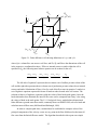
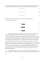
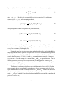
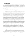
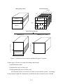
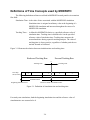
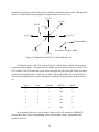
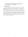
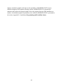
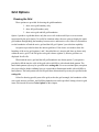
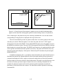
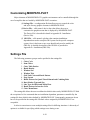
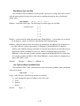
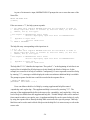
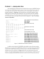
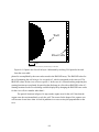
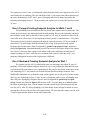
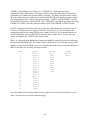
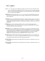
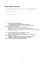
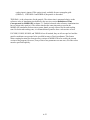
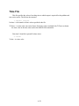
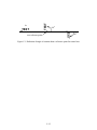
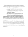
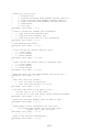
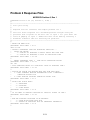
Chapter 2: Particle Tracking Methodology
Main Index
<< Back
Chapter Topics
Qz
z
y
Previous Page
Next Page
Exit
Qy
( x 2, y 22, z 2 )
2
∆y
x
∆x
Qx
Qx
1
2
∆z
j
( x 1, y 1, z 1 )
Qy
i
Qz
1
k
1
Figure 2-1. Finite-difference cell showing definitions of x-y-z and i-j-k
where Q is a volume flow rate across a cell face, and ∆x, ∆y, and ∆z are the dimensions of the cell
in the respective coordinate directions. If flow to internal sources or sinks within the cell is
specified as Qs, the following mass balance equation can be written for the cell,
( nv x − nv x )
2
∆x
1
+
( nv y − nv y )
2
∆y
1
+
( nv z − nv z )
2
∆z
1
=
Qs
∆x∆y∆z
3
The left side of equation 3 represents the net volume rate of outflow per unit volume of the
cell, and the right side represents the net volume rate of production per unit volume due to internal
sources and sinks. Substitution of Darcy’s law for each of the flow terms in equation 3 results in a
set of algebraic equations expressed in terms of heads at nodes located at the cell centers. The
solution of that set of algebraic equations yields the values of head at the node points. Once the
head solution has been obtained, the intercell flow rates can be computed from Darcy’s law using
the values of head at the node points. The U. S. Geological Survey modular three-dimensional
finite-difference ground-water flow model, commonly known as MODFLOW, solves for head and
calculates intercell flow rates (McDonald and Harbaugh, 1988).
In order to compute path lines, a method must be established to compute values of the
principal components of the velocity vector at every point in the flow field based on the intercell
flow rates from the finite difference model. The algorithm described in this report uses simple
2-3