Download LinSig Version 3 user Guide

3.1 The LinSig Traffic Model | 37
3.1.1.5. Queuing
The queue lengths calculated by cyclic flow profile models are often misunderstood and it is
important to understand the different queue components and how they are used to predict
queue lengths.
Queues are inherently difficult to model accurately regardless of the quality or level of detail
used in the model. Predicted queue lengths are extremely sensitive to small changes in input
data. For example looking at a typical Lane in a LinSig model with a flow of 600 PCU, its
predicted queue at a degree of saturation of 90% is 19 PCU. Increasing the flow by 10%
gives a degree of saturation of saturation of 100% and a queue of 29 PCU – an increase of
over 50% in the queue length.
Due to the variability of queues and sensitivity to small changes in conditions both in models
and in reality we recommend avoiding directly calibrating models to measured queues as
unless done with extreme care and highly detailed data it has the potential for introducing
significant inaccuracy into the model. It is recommended that a greater emphasis is placed
on ensuring capacities are modelled correctly whilst still checking that modelled queues are
acceptable.
LinSig models queue lengths in three components similar to those used to model delay.
Uniform Queuing
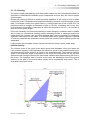
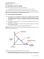
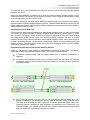
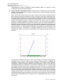
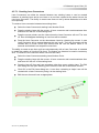
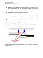
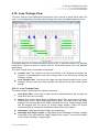
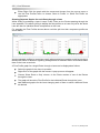
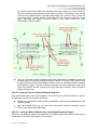
The Uniform queue is the cyclic queue which grows and dissipates every cycle when the
Lane is below capacity. LinSig calculates the maximum queue in the modelled typical cycle
and assumes this will be same for all cycles in the modelled period. The maximum Uniform
queue is the maximum length of the back of the queue as LinSig allows for the fact that
vehicles are still joining the back of the queue after vehicles have started leaving the front of
the queue. The maximum back of queue occurs when the discharging front of the queue
catches up the back of the queue which usually will be lengthening more slowly. This is
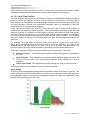
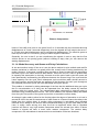
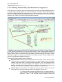
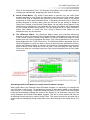
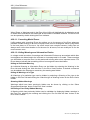
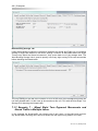
illustrated in the figure below.
Ver. 3.2.10 | January 2013