1
LINEAR–RESPONSE PROGRAM PACKAGE ”LMTO
MAGNONS”
USER’s MANUAL
S.Yu.SAVRASOV
Max-Planck Institute fuer Festkoerperforschung, D-70569 Stuttgart, Germany.
Department of Physics and Astronomy, Rutgers University, Piscataway, NJ 08854.
October 13, 2000
Contents
1 INTRODUCTION
2
2 INSTALLATION
4
3 RUNNING MAGASA/MAGPLW PROGRAMS
3.1 Configuring MAGASA/MAGPLW . . . . . . . . . . . . . . . . . . . . . . . . . . . . .
3.2 Terminal input . . . . . . . . . . . . . . . . . . . . . . . . . . . . . . . . . . . . . . . .
4
5
6
4 MAIN CONTROL FILE: INIFILE
4.1 Control Parameters . . . . . . . . . . . . . .
4.2 Exchange-correlation functional . . . . . . .
4.3 Iterative Procedures Limits and Accuracies
4.4 Atomic Data . . . . . . . . . . . . . . . . .
4.5 Input Control Files: . . . . . . . . . . . . .
4.6 Other Data for MAG-pack . . . . . . . . . .
4.7 Notes to k-space integration . . . . . . . . .
.
.
.
.
.
.
.
.
.
.
.
.
.
.
.
.
.
.
.
.
.
.
.
.
.
.
.
.
.
.
.
.
.
.
.
.
.
.
.
.
.
.
.
.
.
.
.
.
.
.
.
.
.
.
.
.
.
.
.
.
.
.
.
.
.
.
.
.
.
.
.
.
.
.
.
.
.
.
.
.
.
.
.
.
.
.
.
.
.
.
.
.
.
.
.
.
.
.
.
.
.
.
.
.
.
.
.
.
.
.
.
.
.
.
.
.
.
.
.
.
.
.
.
.
.
.
.
.
.
.
.
.
.
.
.
.
.
.
.
.
.
.
.
.
.
.
.
.
.
.
.
.
.
.
.
.
.
.
.
.
.
.
.
.
.
.
.
.
8
9
9
10
11
12
14
15
5 LINEAR–RESPONSE CONTROL FILE: LRTFILE
17
6 EXECUTING MAGASA/PLW IN PARALLEL REGIME
19
7 OUTPUT MESSAGE FILE: OUTFILE
7.1 Reading Input Data . . . . . . . . . . .
7.2 Preparing Structure Constants . . . . .
7.3 Finding Full Potential . . . . . . . . . .
7.4 Calculating Energy Bands . . . . . . . .
7.5 Integrating over Brillouin Zone . . . . .
7.6 Preparing Integration Weights . . . . . .
7.7 Calculating Induced Potential . . . . . .
.
.
.
.
.
.
.
1
.
.
.
.
.
.
.
.
.
.
.
.
.
.
.
.
.
.
.
.
.
.
.
.
.
.
.
.
.
.
.
.
.
.
.
.
.
.
.
.
.
.
.
.
.
.
.
.
.
.
.
.
.
.
.
.
.
.
.
.
.
.
.
.
.
.
.
.
.
.
.
.
.
.
.
.
.
.
.
.
.
.
.
.
.
.
.
.
.
.
.
.
.
.
.
.
.
.
.
.
.
.
.
.
.
.
.
.
.
.
.
.
.
.
.
.
.
.
.
.
.
.
.
.
.
.
.
.
.
.
.
.
.
.
.
.
.
.
.
.
.
.
.
.
.
.
.
.
.
.
.
.
.
.
.
.
.
.
.
.
.
.
.
.
.
.
.
.
.
.
.
.
.
.
.
20
20
22
23
23
24
25
26
7.8
7.9
Calculating Induced Charge Density . . . . . . . . . . . . . . . . . . . . . . . . . . . .
Calculating Susceptibility . . . . . . . . . . . . . . . . . . . . . . . . . . . . . . . . . .
27
28
8 PARAMETER FILE: PARAM.DAT
8.1 Differences with the NMT package . . . . . . . . . . . . . . . . . . . . . . . . . . . . .
8.2 Estimation of the needed core memory . . . . . . . . . . . . . . . . . . . . . . . . . . .
29
29
29
9 ERROR MESSAGES
9.1 Errors connected with PARAM.DAT . . . . . . . . . . . . . . . . . . . . . . . . . . . .
9.2 Errors connected with input . . . . . . . . . . . . . . . . . . . . . . . . . . . . . . . . .
30
30
30
10 USING MAGLIB LIBRARY
10.1 Program QPNT . . . . . . . . . . . . . . . . . . . . . . . . . . . . . . . . . . . . . . . .
31
31
11 Acknowledgments
32
12 COPYRIGHT
32
2
1
INTRODUCTION
The linear–response linear-muffin-tin-orbital (LR-LMTO) programs described here are designed to
perform linear–response calculations of the dynamical spin and charge susceptibilities for arbitrary
wave vectors q + G and frequency ω within the methods of time–dependent density functional theory
(TD–DFT) (Refs. [1, 2, 3, 4]).
The development described here is analogous to the linear–response calculation of the lattice
dynamics and electron–phonon interactions which has been described in several publications [5, 6, 7, 8].
A short description of the method for calculating dynamical susceptibilities is appeared recently [9].
The purpose of the linear–response method is to find change in charge density and magnetization induced by a perturbation of a ceratin wave vector q. If one is interesting by the dynamical
spin or charge susceptibility χ(r, r0 , ω), the perturbation is given by either scalar external potential
δVext (r, t) = δv exp[i(q + G)r + ωt] or external magnetic field.δBext (r, t) = δb exp[i(q + G)r + ωt]
Fixing wave vector q, selecting reciprocal lattice vector G and the frequency ω the problem is reduced
to the self–consistent solution of a differential equation (so–called Sternheimer’s equation) which is a
linearized version of Schr¨
odinger’s equation. Solving this problem self–consistently gives an access to
the function χ(r, q + G, ω) which is the susceptibility Fourier transformed over one index. The entire
problem is very similar to the self–consistency problem of standard band–structure calculation. It is
however much more heavy to solve it numerically because finding χ(r, q + G, ω) for a grid of wave
vectors q + G requires Nq+G (total number of q + G points) self-consistent calculations performed
for a set of frequencies ω. It therefore requires Nq+G × Nω self–consistent calculations, each of them
being equivalent to the standard band structure calculation for the unperturbed system.
Linear–response calculations of χ(r, q + G, ω) should, in principle, not be so sensitive to the
details of the charge density distribution over the cell. However a full–potential (FP) solution of the
problem is desired. According to different treatment of the full–potential terms in the band structure
calculations performed with the original FP-LMTO method (for the description of these programs
see FULL-POTENTIAL LMTO PROGRAMS ”NMT”: USER’s MANUAL, which is available on the
WEB site under the address: http://www.mpi-stuttgart.mpg.de/docs/ANDERSEN/) there are two
linear–response programs: MAGASA and MAGPLW. MAGASA uses atomic sphere approximation
and does not treat interstitial region correctly. MAGPLW uses plane–wave representation for all the
relevant quantities in the interstitial region, and, therefore, much more accurate. Note that MAGPLW
code is much slower than MAGASA program.
The purpose of these MAG* programs is to calculate χ(r, q+G, ω) The basic input to the program
is given by the charge density distribution of the unperturbed crystal. It is therefore necessary to install
and learn how to use the programs NMTASA and/or NMTPLW for the original self–consistent band
structure calculations with the LMTO method, This program uses the same plane–wave representation
for the charge densities and the potentials in the interstitial region. (The package of programs NMT
including three versions NMTASA,NMTCEL and NMTPLW is distributed separately and can be
downloaded from http://www.mpi-stuttgart.mpg.de/docs/ANDERSEN/SAVRASOV/frames.htm)
Finding χ(r, q + G, ω) is divided in two parts which run independently:
• Preparational part: A self–consistent band structure calculation with the NMTASA or NMTPLW
code must be performed for the original crystal. A self–consistent charge density file (SCFFILE)
must be created.
• Self–consistency part: Self–consistent linear–response calculation is performed for each wave
3
vector q + G, frequency ω and for either external scalar potential field (for finding charge susceptibility) or for external magnetic field (for finding spin susceptibility) using the package
MAGASA or MAGPLW. For magnetic field calculation, there is additional parameter µ=-1,0,1
fixing polarization of the field in spherical coordinates. The main input file to the NMT* program INIFILE is used as the main input control file in the MAG*. Also, a list of wave vectors
q + G must be prepared before running MAG* and stored in the file (called PNTFILE). Another input control file (called LRTFILE) must be prepared (typical example will be given).
The change in charge density for each q + G, ω, µ will be calculated by MAG* and stored in two
kinds of files referred as DROFILE and DPSFILE. DROFILE contains change in charge density
expanded in spherical harmonics within MT–spheres and DPSFILE contains change in charge
density expanded in plane waves in the interstitial region. There is as many DROFILEs and
DPSFILEs as 3 × Nq × Natom .
All programs described in this manual can be downloaded from http://www.mpi-stuttgart.mpg.de/docs/AN
About the notations in this document:
• all file names like nbc.ini, main.exe, are boldfaced.
• all directory names like /magplw/dat/ are italicized.
• capitalized names like INIFILE, STRFILE are made to shorten references to the MAIN INPUT
CONTROL FILE (for INIFILE), STRUCTURE CONTROL FILE (for STRFILE), etc.
I apologize if the description of some parameters is short and unclear. Any suggestions to improve
this manual are welcomed. I also cannot guarantee that all the bugs in the programs are found. Since
linear–response calculation is a relatively new field in computational solid–state physics there could
be some other problems, instabilities in the algorithms which have been used in the programs. Any
further improvements of the programs are welcomed.
4
2
INSTALLATION
In this section the directories which are used for running the programs and storing input/output data
are described. The MAG* packages have the directory organization similar to the packages NMT*.
There exists three main directories:
• /magasa/ /magplw/- directories containing source code of the main LR-LMTO programs MAGASA/MAGPLW designed to perform self–consistent linear–response calculations. Input data
files and some auxiliary programs are also stored in this directory.
• /maglib/ - directory containing a number of other application programs helping to construct
input data and understand output information.
Below the contents of each of the directories is described. The /magasa/ and /magplw/ have two
subdirectories:
• /magasa/run/,/magplw/run - directories containing the source code *.f of the main LR-LMTO
programs MAGASA,MAGPLW (text of the program written on FORTRAN77), object files *.o
and executable file usually named as main.exe.
• /magasa/dat/,/magplw/dat/ - directories with the input/output data files to the main LRLMTO program. Usually, many subdirectories are created here according to the element (compound) name to be calculated. An example of the compound which will be considered below is
ferromagnetic iron. The input/output data files are contained in /magplw/dat/fe/ directory.
There exists a library directory /maglib/. It containes a number of auxiliary programs. The
programs understand input/output data files of the MAG* codes. The contents of /maglib/ is
• /maglib/qpnt/ - program which generates irreducible set of q-points according to the input
divisions and stores them into the PNTFILE. The latter is one of the input files to the MAG*
codes. Note that the perturbation wave vectors q must be chosen to have minimal length (one
of the options while running QPNT) in order to have well–convergent plane–wave expansions
(see below).
All programs and data files are tared and gzipped into 2 files named as magasa.tar.gz, magplw.tar.gz, and maglib.tar.gz
1. gunzip magasa.tar.gz
2. tar -x -f magasa.tar
Repeat these steps for magplw.dec, and maglib.dec.
3
RUNNING MAGASA/MAGPLW PROGRAMS
In this section general hints how to run main linear-response codes MAGASA/MAGPLW are described. Section USING MAGLIB LIBRARY will describe how to run auxiliary library routines.
5
3.1
Configuring MAGASA/MAGPLW
To be able to run MAGASA/MAGPLW it is necessary to compile the source data files. A few
comments must be said here. First, the maximum size of every array (such as maximum number
of atoms, lmax , etc) in the program is declared using the Fortran PARAMETER statement. These
statements are contained in the file PARAM.DAT. (See Section PARAMETER FILE: PARAM.DAT
for the detailed description) The file PARAM.DAT is included into every source code during the
compilation time by INCLUDE statement. The second comment concerns a scratch file storage. To
minimize core memory, some data during the run are temporary stored in the scratch files. To be able
to do this, a scratch directory must exist on any particular node where execution of the program is
performed.
To create executable file of the MAG* program, go to the directory /mag*/run/.
1. Edit PARAM.DAT and install the necessary size of arrays. Sample PARAM.DAT file is provided.
2. Edit the file setup.f and specify the path to the scratch directory. Also check that other set-up
data match with your local operational system.
3. Edit the file timel.f and specify the call to the system subroutine to learn CPU time.
4. Compile all programs, link them to get executable file main.exe. Under UNIX, using AIX XL
Fortran Compiler this looks like: xlf -cOw *.f to compile only, with optimization, and suppressing all warning messages. The command xlf -cCg *.f will compile only, suppress optimization
and provide debugging information. To link, use the command xlf *.o -o main.exe. To create
a load map use the command xlf *.o -o main.exe -bloadmap:map. At the end of the map
file a total amount of the core memory allocated by the program is printed out.
To run MAG* for a particular compound, create a subdirectory in /mag*/dat/. For example, to
calculate χ of Fe, create /magplw/dat/fe/. In this subdirectory, create the following subdirectories
(this is default list of the subdirectories listed in the linear-response control file LRTFILE. See also
chapter LINEAR RESPONSE CONTROL FILE: LRTFILE.)
• /magplw/dat/fe/INP/ subdirectory for storing input files, like main input control file INIFILE,
structure control file STRFILE, self–consistent charge density file SCFFILE, linear response
control file LRTFILE, etc.
• /magplw/dat/fe/DRO/ subdirectory for storing the files with changes in charge density and
pseudodensity. All names for these files will be given automatically.
• /magplw/dat/fe/WGT/ subdirectory for storing the files containing the k space integration
weights. All names for these files will be given automatically.
Note that the directory INP contains the files which are unique for all q + G points and frequencies
ω. All other directories contain the files which are specific for any particular q+G point, ω and
field polarization. Since there are too many files (4 × Nq+G × Nω ) their filenames are constructed
automatically. For example, the rule to construct the name for DROFILE is (i) three first letters
are dro, (ii) q–point number, (iii), G-vector number, (iv) ω, (v) polarization. Polarization µ=-1
abbreviated as ”m”, µ=0 abbreviated as ”z”, and µ=+1 abbreviated as ”p”. If scalar potential
6
field is used for charge susceptibility, it is abbreviated as ”v”. For example, when one finds selfconsistent response for the q–point number 12 (listed in PNTFILE), G-vector 3, ω = 30 meV, and
polarization z along magnetization axis, the change in charge density (DROFILE) will be stored in
the file dro12g03w30z and will be automatically placed into the directory DRO. Analogously names
are constructed for DPSFILEs, etc.
3.2
Terminal input
MAGASA/MAGPLW programs have several input lines:
IFOLDER?
INIFILE?
SCFFILE?
STRFILE?
LRTFILE?
Q-POINT?
G–SHELL?
FREQUEN?
RUNMODE?
RUNTASK?
The answers must be either given from the terminal or placed into a job file. General description
of the input lines is given below:
• IFOLDER gives the subdirectory name where all input files are stored. For example, if the input
subdirectory is called INP/, the string ”INP/” must be given to the answer ”IFOLDER?”.
• INIFILE is a name of the main control data file. The structure of the file is identical to the
INIFILE of the NMT package. A description of this file and its difference to that of the NMT
package will be given in section MAIN CONTROL FILE: INIFILE. INIFILE must be stored in
the subdirectory specified by the parameter IFOLDER.
• SCFFILE is a name of the self-consistent charge density file which is calculated by the NMTASA/PLW packages. SCFFILE must be stored in the subdirectory specified by the parameter
IFOLDER.
• STRFILE is a name of the structure data file. It is the same as used by the NMT* package,
therefore it is not described in this manual. STRFILE must be stored in the subdirectory
specified by the parameter IFOLDER.
• LRTFILE is a name of the linear-response control file. This file is specific for linear response
calculation and does not contain any information about the compound. Its detailed description
will be given below in the section LINEAR RESPONSE CONTROL FILE: LRTFILE. LRTFILE
must be stored in the subdirectory specified by the parameter IFOLDER.
• Q-POINT is a q–point number. A list of q points must be prepared and stored in the PNTFILE.
Use program QPNT located in /maglib/qpnt/ for this purpose. (See section USING MAGLIB
LIBRARY for the detailed description). Lines in the PNTFILE numerate q points. A path
to the PNTFILE is contained in the INIFILE. Therefore setting Q-POINT number from the
terminal will result in reading the corresponding line from the PNTFILE. Note that Q-POINT
7
number must be set as a character string. The reason is that all output files containing change in
charge densities, potentials, etc, must be named differently for different q points. The character
string specifying q point will be added to any output filename. For example,
Q-POINT? 01
means that the first point from PNTFILE will be treated as a perturbation wave vector and the
string 01 will be added to any of the output files.
• G-SHELL shows which of the reciprocal lattice vectors will be added to q–point in order to
make a perturbation vector q + G. Reciprocal lattice vectors are generated by shells in the
reciprocal space and stored in the PNTFILE. G-SHELL=0 corresponds to G=0, then follows
first, second, etc. shells. Setting G–SHELL equal to 1 will consider a given q–point plus all
reciprocal lattice vectors G which belong to a given shell as perturbation vectors q+G. Some of
these vectors can be connected by symmetry operations. Note that G6= 0 are only necessary to
apply external fields changing within the unit cell. All acoustic magnon modes, for example, are
seen by considering only q with G=0. To find optical magnon modes, it is necessary to apply
non–zero G.
• FREQUEN gives the frequency in meV. Note that FREQUEN must be set as a character string.
The reason is that all output files containing change in charge densities, potentials, etc, must be
named differently for different ω The character string specifying ω will be added to any output
filename. For example,
FREQUEN? 0300
means that ω = 300 meV will be treated as the perturbation frequncy and the string 0300 will
be added to any of the output files.
• RUNMODE shows in which mode the program will be executed. The following answers can be
given:
– 0 : preparational mode. Only the bands for a large number of k-points will be calculated.
Use this mode when calculating metals. For correct treatment of the effects of the Fermi
surface, the knowledge of the energy bands at a dense grid is required. This mode will
prepare the necessary file.
– 1 : starting self–consistency mode. Use this mode when nothing is done with the self–
consistency for a given q point. That means that the change in charge density is not known
(no DROFILE and DPSFILE exist)
– 2 : continuation of the self–consistency. Use this mode when self–consistency for a given q
point is continuing with the same set up (# of k points and other data were not changed).
DROFILE and DPSFILE must exist at this step, but by some reason self–consistency is not
finished. Actually, if one sets RUNMODE=2 and the program will not find corresponding
DROFILE and DPSFILE, the mode will be automatically set to one.
• RUNTASK selects polarizations: m,z,p stand for applied magnetic fields polarized along -1,0,1
axis. Note that the magnetization axis is always given by z–axis. Therefore in order to study
transverse spin fluctuations in ferromagnets, only m and p polarizations should be considered.
Another keyword v stands for applied scalar external potential in order to study charge response.
8
4
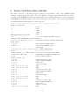
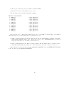
MAIN CONTROL FILE: INIFILE
The main control file of the linear-response package is very similar to that of the NMTASA/PLW
packages. It has an extension .ini. Below an example of magnon spectrum calculation for Fe is
considered. The INIFILE for Fe has the name fe.ini or more shortly ini. It can be created easily from
the INIFILE of the NMT package. Only a few lines must be edited there. Let’s consider this example:
*** Band Structure Calculation of bcc-Fe ***
---------------------------------------------------------------Control Parameters :
3
- lift
1
- lmto
0
- nsph
1
- lrwf
0
- npfr
Exchange-Correlation Code :
14
- 1,2,3 :by VBarth-H;Gunn-L;Jan-W
Iterative Procedure Limits and Accuracy :
50,0.2,0.2,1.D-4,+6 0,0.3,0.3 - niter,mix,mag,eps,lbr,ibr,mixb,mixh
Atomic Data :
1,1,2,1
- natom,nsort,nspin,norbs
5.425,1.0
- lattice parameter,v/v0
1
- is(iatom)
3 (-0.05,0.0),(-1.0,0.0),(-2.5,0.0) - Nkap, Ekap(ikap)
for Fe
----------------------26.D0 18.D0,1,1,0,0.5D0,55.847 - z zcor,lr,icor,ispl,split,mass
2.349,1.D0,1.D0,0.D0
- mt-sphere,rou-sphere,weight,rloc
6 2 6
- lmax-t,lmax-b,lmax-v
valence states are :
s p d f
- states for E=0.5 Ry
4 4 3 4
- main quantum numbers
1 1 1 0
- basis set
3 3 3 0
- choice of Eny
0.30, 0.30, 0.30, 0.50
- Eny
0.30, 1.60,-1.50,-3.00
- Dny
s p d f
- states for E=0.5 Ry
4 4 3 4
- main quantum numbers
1 1 1 0
- basis set
3 3 3 0
- choice of Eny
0.30, 0.30, 0.30, 0.50
- Eny
0.30, 1.60,-1.50,-3.00
- Dny
s p d f
- states for E=0.5 Ry
4 4 3 4
- main quantum numbers
1 1 1 0
- basis set
3 3 3 0
- choice of Eny
0.30, 0.30, 0.30, 0.50
- Eny
9
0.30, 1.60,-1.50,-3.00
- Dny
semicore states are :
0
- # of states
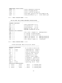
Input Control Files :
----------------------2 ’fe.con’
- icon,<confile>
0 ’fe.tmp’
- itmp,<tmpfile>
2 ’fe.psi’
- ipsi,<psifile>
0 ’fe.tmp’
- itmp,<tmpfile>
2 ’fe.bnd’
- ibnd,<bndfile>
0 ’fe.pot’
- ipot,<potfile>
0 ’fe.ptn’
- iptn,<ptnfile>
0 ’fe.dos’
- idos,<dosfile>
2 ’fe.scf’
- iscf,<scffile>
2
’out’
- iout,<outfile>
Other Data for Mag-Pack :
0,9,0.1
- nff,nef,de
16,16,16,32
- n1,n2,n3,nc
20,20,20,0.02,0.04,0,10
- nfft1,nfft2,nfft3,epsr,epsg,kbz,bzr
Additional input files:
0 ’fe.hub’
- ihub,<hubfile>
0 ’fe.hop’
- ihop,<hopfile>
0 ’fe.opt’
- iopt,<optfile>
2 ’fe.enr’
- ienr,<enrfile>
2 ’fe.pnt’
- ipnt,<pntfile>
This file is unique and is used to perform self–consistent calculations for all q,G,ω, µ. Only a few
lines are treated differently from the input to NMTASA/PLW programs. It will be explained below:
4.1
Control Parameters
*** Band Structure Calculation of bcc-Fe ***
---------------------------------------------------------------Control Parameters :
3
- lift
1
- lmto
0
- nsph
1
- lrwf
0
- npfr
This set of parameters should be exactly the same as used in the NMTASA/PLW calculation.
Note that the keyword lrwf should be set to 1 when preparing the SCFFILE by NMTASA/PLW.
4.2
Exchange-correlation functional
Exchange-Correlation Code :
14
...
- 1,2,3 :by VBarth-H;Gunn-L;Jan-W
10
The exchange–correlation should be the same as used in the NMTASA/PLW calculation.
4.3
Iterative Procedures Limits and Accuracies
Iterative Procedure Limits and Accuracy :
50,0.2,0.2,1.D-4,+6 0,0.3,0.3 - niter,mix,mag,eps,lbr,ibr,mixb,mixh
This set of parameters has the same meaning as in the NMTASA/PLW calculation, but they are
used for calculating changes in charge density. The meaning of every parameter is given below:
• niter: max. number of iterations for doing self-consistency of the change in charge density for
given q,G,ωµ.
• mix: starting mixing of the charge density in linear mixing scheme. During the iterations
towards self–consistency the mixing will be optimally adjusted according to the Pratt scheme.
This parameter is ignored if Broyden mixing (see below) is switched on.
• mag: starting mixing for the magnetization in linear mixing scheme. During the iterations towards self-consistency the magnetization mixing will remain constant and will NOT be adjusted.
The parameter has no effect for non–spin–polarized calculations or if Broyden mixing (see below)
is switched on.
• eps: charge density convergency criterion. Typically 10−2 . The program will stop doing self–
consistency for a particular q,G,ωµ.if the mean square difference between two induced densities
in consequent iterations is less then eps. Note that if a few displacements and polarizations run
spontaneously, the program will automatically terminate iterating those displacements which
reach self–consistency. Also note that the reached convergency is written to the DROFILE.
When restarting the execution, the program will check whether for a given displacement and
polarization reached accuracy is higher than input eps or not. If it is higher, number of iterations
for this displacement and polarization will be automatically set to 0, if it is not, then the
iterational cycle will continue. You can also use this when it is necessary to improve convergency
of the induced charge density. Suppose it is self–consistent with the accuracy, say, 10−2 . In order
to improve the convergency, reset eps from 10−2 to, say, 10−4 in the INIFILE. The iterational
cycle for given displacement and polarization will be renewed.
• lbr: switches on the Broyden mixing. If -1 then Broyden is OFF, if 0 then Broyden is ON for
l=0 component of δρ(r), if +1,+2 then Broyden is on for l.le.lbr component of Drho(r). It is
highly recommended to set lbr to the lmax value of spherical harmonics expansions for the charge
density and potential. It is controlled by the parameter LmaxV (see below) and it is usually 4
(for ASA) or 6 (for PLW). Broyden restarts every time after NTERMAX iterations. Parameter
NTERMAX is in PARAM.DAT. Usually NTERMAX=15.
• ibr starts Broyden after I=ibr iterations. If ibr=0 then start immediately. If ibr>0 then first
I=ibr iterations will be done with the linear mixing scheme where the mixing parameters mix
and mag are specified above.
• mixb: this is initial guess for Jacobian which is closely related to mixing parameter mix in the
linear mixing scheme. It was found that mixb cannot be small and it is usually of the order
0.3-0.4
11
• mixh: this is linear mixing parameter for higher l-components (l>lbr) of the charge density.
Since it is assumed that these components do not influence much the self-consistence loop, they
are mixed within linear mixing scheme and do not stored for all previous iterations.
4.4
Atomic Data
Atomic Data :
1,1,2,1
- natom,nsort,nspin,norbs
5.425,1.0
- lattice parameter,v/v0
1
- is(iatom)
3 (-0.05,0.0),(-1.0,0.0),(-2.5,0.0) - Nkap, Ekap(ikap)
This set of parameters should be exactly the same as used in the NMTASA/PLW calculations.
Note that an option switching spin-orbit coupling is not yet available for the linear–response magnon
program. Note also that number of spins must ALWAYS be set to 2 when using MAGASA/PLW.
for Fe
26.D0 18.D0,1,1,0,0.5D0,55.847
2.349,1.D0,1.D0,0.D0
6 2 6
----------------------- z zcor,lr,icor,ispl,split,mass
- mt-sphere,rou-sphere,weight,rloc
- lmax-t,lmax-b,lmax-v
This set of parameters should be the same as used in the NMTASA/PLW calculation.
• for Nb: title for every atom. Note that this character string (maximum 10 letters) will be read
and widely used in the output file. Therefore it is recommended to use the format ”for EL”
• z: atomic number.
• zcor: deep-core charge.
• lr:
– 0 for non-relativistic calculations,
– 1 for scalar-relativistic valence states
• icor: this parameter has no effect for linear–response calculation.
• ispl,split: both these parameters have no effect for linear–response calculation.
• mass: atomic mass of the element as in the periodic table.
• mt-sphere: non-touching muffin-tin sphere radius.
• rou-sphere: this parameter has no effect for linear–response calculation using MAGASA/PLW
packages.
• weight: this parameter has no effect for linear–response calculation.
• rloc: this parameter has no effect for linear–response calculation.
12
• lmax-t: maximal angular momentum l (not l + 1 !) for the basis functions (i.e. for the decomposition of the tails coming from other atoms). Normally it is 6 for PLW calculation.
• lmax-b: maximal l actually included in basis.
• lmax-v: maximal l-value for the expansion of the induced charge density and the induced potential in spherical harmonics. Normally it is the same as lmax-t.
The following block is repeated for each κ from 1 to nkap:
valence states are :
s p d f
4 4 3 4
1 1 1 0
3 3 3 0
0.30, 0.30, 0.30, 0.50
0.30, 1.60,-1.50,-3.00
s p d f
4 4 3 4
1 1 1 0
3 3 3 0
0.30, 0.30, 0.30, 0.50
0.30, 1.60,-1.50,-3.00
s p d f
4 4 3 4
1 1 1 0
3 3 3 0
0.30, 0.30, 0.30, 0.50
0.30, 1.60,-1.50,-3.00
-
states for E=0.5 Ry
main quantum numbers
basis set
choice of Eny
Eny
Dny
states for E=0.5 Ry
main quantum numbers
basis set
choice of Eny
Eny
Dny
states for E=0.5 Ry
main quantum numbers
basis set
choice of Eny
Eny
Dny
The meaning of these parameters is exactly the same as in the INIFILE of the NMT package.
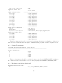
4.5
Input Control Files:
Input Control Files :
2 ’fe.con’
0 ’fe.tmp’
2 ’fe.psi’
0 ’fe.tmp’
2 ’fe.bnd’
0 ’fe.pot’
0 ’fe.ptn’
0 ’fe.dos’
2 ’fe.scf’
2
’out’
----------------------- icon,<confile>
- itmp,<tmpfile>
- ipsi,<psifile>
- itmp,<tmpfile>
- ibnd,<bndfile>
- ipot,<potfile>
- iptn,<ptnfile>
- idos,<dosfile>
- iscf,<scffile>
- iout,<outfile>
This section gives the names of the files which are used by the program. The consequence of the
files is the same as in the INIFILE of the NMT* programs. The meaning of the control parameters is
the following:
13
• 0 - file is not created, or created as temporary.
• 1 - file will be opened as a new one and saved, if file exists, the execution will be terminated.
• 2 - file already exists and will be read, if file does not exist, the switch will be automatically set
to 1.
• 6 - the contents of the file will be printed out to the terminal. (channel #6)
• icon,<confile>: this is the structure constants file which will be created by MAGASA/PLW
at the beginning. Note that the CONFILE created by MAGASA/PLW cannot be used by the
program MAGASA/PLW. Keep structure constants in the INP directory to make them shareable
when running different q points spontaneously. Always set icon=2.
• itmp,<tmpfile>: this parameter is not used by MAGASA/PLW.
• ipsi,<psifile>: this is the file which contains wave functions on the grid of k points in the IBZ.
Keep wave functions in the INP directory to make them shareable when running different q
points spontaneously. Always set ipsi=2.
• iscr,<scrfile>: this is the first character string for the scratch file names. Scratch files will be
created in the temporary directory. The path to the temporary directory is contained in the file
/mag*/run/setup.f. Always set iscr=0.
• ibnd,<bndfile>: this is the file which contains energy bands on the grid of k points in the IBZ.
Keep energy bands in the INP directory to make them shareable when running different q points
spontaneously. Always set ibnd=2.
• ipot,<potfile>: this file is not used by MAGASA/PLW.
• ifat,<fatfile>: this file is not used by MAGASA/PLW.
• idos,<dosfile>: this file is not used by MAGASA/PLW.
• iscf,<scffile>: this file is not used by MAGASA/PLW. Name for the SCFFILE which contains
the self-consistent charge density distribution for the original crystal as calculated by the program
NMTASA/PLW, will be read from the terminal. SCFFILE must be prepared before running
linear–response code! For convenience, place it into the INP directory.
• iout,<outfile>: this is the current output file in this run. In fact, it is first character string of the
filename. The final name will also contain q–point number as it was read from the Q-POINT
input line, frequency name as read from FREQUEN input line, and also task name, as it was
read from the RUNTASK input line. Set iout=2 if storage is necessary, set iout=6 to print the
current output to the terminal. Note that this file will be created NOT in the INP directory as
it is done with CONFILE,BNDFILE, and PSIFILE, but in the root directory.
14
4.6
Other Data for MAG-pack
Other Data for Mag-Pack :
0,9,0.1
16,16,16,32
20,20,20,0.02,0.04,0,10
- nff,nef,de
- n1,n2,n3,nc
- nfft1,nfft2,nfft3,epsr,epsg,kbz,bzr
This set of parameters is similar to what is used in the NMTPLW calculation. However there are
differences. The exact meaning is given below:
• nff,nef : number of filled bands in the main valence panel (above the semicore!) and number of
bands crossing the Fermi level. These parameters must be chosen with more care in contrast to
NMTPLW, see subsection ”Notes to k-space integration” for the detailed description.
• pole: parameter connected with the Lorentizan broadening of the Fermi surface integrals. The
parameter is not used by NMTPLW. See also subsection ”Notes to k-space integration”.
• nk1, nk2, nk3: divisions of the Brillouin zone along three directions for the tetrahedron integration. (see subsection ”Notes to k-space integration”).
• nw1: divisions of the Brillouin zone along three directions for finding the weights in the tetrahedron integration. Only the first division must be specified, two others nw2, nw3 will be
calculated according to nk1, nk2, nk3. Note that this parameter substitutes the parameter nc
of the NMTPLW. See subsection ”Notes to k-space integration” for the detailed description.
• m1, m2, m3: divisions of the unit cell for the fast Fourier transform. These parameters should
be the same as used by the NMTPLW calculation.
• epsR, epsG : accuracy of matching the spherical Hankel functions in real and reciprocal space.
These parameters should be the same as used by the NMTPLW calculation.
• keyt, bzr: to accelerate Fourier transforms when calculating interstitial potential matrix elements, set keyt=1. In this case the radius of the cutoff sphere in reciprocal space is set by
parameter bzr times the radius of the sphere circumscribing the Brillouin zone. Usually it is 4-6.
The smaller bzr value the faster calculation the lower the accuracy. These parameters should be
the same as used by the NMTPLW calculation.
Finally, path to additional input files must be specified
Additional input files:
0 ’fe.hub’
0 ’fe.hop’
0 ’fe.opt’
2 ’fe.enr’
2 ’fe.pnt’
-
ihub,<hubfile>
ihop,<hopfile>
iopt,<optfile>
ienr,<enrfile>
ipnt,<pntfile>
• ihub,<hubfile>: this parameter has no effect in the linear-response calcualtion.
• ihop,<hopfile>: this parameter has no effect in the linear-response calcualtion.
15
• iopt,<optfile>: this parameter has no effect in the linear-response calcualtion.
• ipnt,<pntfile>: this is the file which contains a list of the wavevectors q for linear–response
calculations (so called PNTFILE). Use program QPNT located in /maglib/qpnt/ to prepare
PNTFILE. (See section USING MAGLIB LIBRARY for the detailed description). Lines in the
PNTFILE numerate q points. Therefore setting Q-POINT number from the terminal will result
in reading the corresponding line from the PNTFILE. For convenience, place it into the INP
directory. Always set ipnt=2.
• ienr,<enrfile>: this is the file which contains energy bands on the dense grid of k points in the
IBZ (see subsection ”Notes to k-space integration”). Keep energy bands in the INP directory to
make them shareable when running different q points spontaneously. Always set ienr=2.
4.7
Notes to k-space integration
This section explains how to handle with the parameters responsible for the k–space integration which
is performed to find change in charge density for every vector q. This set of parameters involves nff,
nef - number of bands below and crossing the Fermi level, pole - Lorentzian broadening, nk1,nk2,nk3 BZ divisions for integration, nw1,nw2,nw3 - BZ divisions to find the integration weights, and <enrfile>
- file which contains energy bands generated at the grid set up by nw1,nw2,nw3.
For semiconductors, when there is an energy gap between occupied and unoccupied states, the k–
space integration using misweight–free tetrahedron method is equivalent to the special point method.
In this case set nff to the actual number of bands below the Fermi energy, nef to zero, pole to zero,
specify the grid parameters nw1,nw2,nw3 equal to the BZ divisions nk1,nk2,nk3. ENRFILE which
contains the bands generated at the grid nw1,nw2,nw3 will be the same as the BNDFILE which
contains the bands generated at the grid nk1,nk2,nk3. These files will be created automatically after
one run of the main program.
For metals, it is possible (without lost of computer time) to essentially improve accuracy of the BZ
integration using multigrid technique. The idea is based on the fact that the effects of energy bands
and of the Fermi surface can be taken into account exactly in the linear–response calculation. While
matrix elements necessary to construct induced charge density are calculated at the coarse grid (set
up by the numbers nk1,nk2,nk3), the weights for the k–space integration which take into account the
exact shape of the Fermi surface can be found using the bands generated at the dense grid (set up by
the numbers nw1,nw2,nw3). Two grids must commensurate with each other. To reach this purpose,
first ENRFILE which contains the bands at the dense grid must be created. To create ENRFILE, just
specify RUNMODE=0. The program will automatically generate k points according to nw1,nw2,nw3,
will do only one band calculation, will store ENRFILE and will stop. Using any RUNMODE different
from 0 will pick up coarse k–space grid according to nk1,nk2,nk3. During the construction of the
weights for the integration, information stored in the ENRFILE will be taken into account.
In order to choose numbers of bands below and crossing the Fermi level, use the following hint.
Look at the bands in the Γ point. (They usually printed out in the OUTFILE). Locate the band
nearest to the Fermi energy. Step out from this band by approximately 0.5 Ry down. Count the
bands below this energy, they can be treated as filled bands nff. The bands located at the energy
window plus/minus 0.5 Ry from the Fermi energy should be treated as the bands crossing EF (nef).
Set lorentizan broadening parameter pole to approximately 0.1 Ry.
16
Note that any wave vector q must belong to the grid generated by nk1,nk2,nk3 and nw1,nw2,nw3.
In other words, grid of wave vectors q set-up by three numbers nq1,nq2,nq3 (see section USING
MAGLIB LIBRARY) must commensurate with the grids nk1,nk2,nk3 and nw1,nw2,nw3. Normally,
select such nq1,nq2,nq3 when the number of irreducible q points generated is not more than 20-40.
The grid for k–space integration can be the same (nk1,nk2,nk3=nq1,nq2,nq3) or not more than twice
denser. Do not use very many k points here, all k–space integrals are fastly convergent. The grid
nw1,nw2,nw3 is the same as the grid nk1,nk2,nk3 for semiconductors. For metals, use nw1,nw2,nw3
which is 3-5 times denser than the grid nk1,nk2,nk3. The number of irreducible k points for integration
weights should be of the order 1000.
Final note must be said when calculating electron–phonon matrices (RUNMODE=5). Since the
corresponding BZ–integrals are very sensitive to the divisions nk1,nk2,nk3 use the following hints.
(i) Reach self–consistency for all q–points, all displacements and all polarizations. All DROFILEs
and DPSFILEs must be created and stored in the DRO directory. (Calculate dynamical matrix
and the phonon spectrum for every q–point when for this q–point self–consistency is reached for all
displacements and all polarizations). (ii) Delete contents of the directory WGT which contains the
weights for the BZ integration. (iii) Make a new INIFILE in which specify the divisions nk1,nk2,nk3
of the coarse grid equal to the divisions nw1,nw2,nw3 of the dense grid, the number of irreducible k
points for integration must be of the order 1000. Carefully set the number of bands below/crossing
the Fermi level equal to the actual number of bands below/crossing the Fermi level. Delete or rename
BNDFILE and CONFILE since they contains the information generated for the coarse grid. (iv) Run
the main program with the RUNMODE=5. CONFILE and BNDFILE will be created. Also a new
PSIFILE with the wave functions will be created. However, the wave functions will be stored only for
the bands crossing the Fermi level (that’s why it is necessary to reset this number, otherwise this file
will have a huge size!). (v) After CONFILE, BNDFILE, and PSIFILE are created at the dense grid
nk1,nk2,nk3=nw1,nw2,nw3, run different q points to calculate the electron–phonon matrices. The new
weight files will be created automatically and stored in the WGT directory. Note that the integration
weights for the electron–phonon matrices are different from those which have been using to find the
induced charge densities, that’s why it is necessary to delete the contents of the directory WGT before
using RUNMODE=5. The calculation of the electron–phonon matrix is computationally much more
faster than making self–consistency and finding dynamical matrix.
17
5
LINEAR–RESPONSE CONTROL FILE: LRTFILE
LRTFILE is used to set up the data which are specific for linear response calculations. In fact, this
file does not contain an information on the compound to be calculated and, therefore, the LRTFILE
does not have to be modified except some special cases. A typical LRTFILE is given below:
SET-UP DATA FOR LINEAR RESPONSE CALCULATIONS
----------------------------------------------------GENERAL SETTINGS:
’Magnons
’
- Response scheme (Phonons/Magnons)
’Plz=off’
- Polarizabilty on/off
’Stn=off
’
- Stoner renormalization on/off
’Del=on
’
- Changes in radial functions on/off
’Dyn=none ’
- Dynamical matrix scheme (none,hf,oka1,oka*)
DEFAULT FILE SETTINGS:
0 ’DSF/dsf’
- idsf,<dsffile>
2 ’WGT/wgt’
- iwgt,<wgtfile>
0 ’TMP/tmp’
- itmp,<tmpfile>
0 ’STN/stn’
- istn,<stnfile>
0 ’PHN/phn’
- iphn,<stnfile>
0 ’PLZ/plz’
- iplz,<plzfile>
0 ’PLZ/pls’
- ipls,<plsfile>
0 ’POT/dsv’
- idsv,<dsvfile>
0 ’POT/dpv’
- idpv,<dpvfile>
2 ’DRO/dro’
- idro,<drofile>
2 ’DRO/dps’
- idps,<dpsfile>
OTHER INPUT DATA:
0.0D0 0.03D0 30
- Wmin,Wmax,Nomg
There several sections in it. Section GENERAL SETTINGS describes linear-response control
parameters.
GENERAL SETTINGS:
’Magnons
’
’Plz=off’
’Stn=off
’
’Del=off
’
’Dyn=none ’
}
-
Response scheme (Phonons/Magnons)
Polarizabilty on/off
Stoner renormalization on/off
Changes in radial functions on/off
Dynamical matrix scheme (none,hf,oka1,oka*)
• Response scheme: This string must be set to Magnons. Other option ”Phonons” is used by the
program PHNPLW
• Polarizability: Plz=off key must be used
• Stoner renormalization is not used by the MAGASA/PLW program.
18
• Changes in radial wave functions must be switched OFF.
• Dynamical matrix scheme must be set to none.
The following section is called default file settings:
DEFAULT FILE SETTINGS:
0 ’DSF/dsf’
2 ’WGT/wgt’
0 ’TMP/tmp’
0 ’STN/stn’
0 ’PHN/phn’
2 ’PLZ/plz’
2 ’PLZ/pls’
0 ’POT/dsv’
0 ’POT/dpv’
2 ’DRO/dro’
2 ’DRO/dps’
-
idsf,<dsffile>
iwgt,<wgtfile>
itmp,<tmpfile>
istn,<stnfile>
iphn,<stnfile>
iplz,<plzfile>
ipls,<plsfile>
idsv,<dsvfile>
idpv,<dpvfile>
idro,<drofile>
idps,<dpsfile>
Since there is a lot of different files which are stored for every q,G,ω, µ it is useful to sort them in
different subdirectories. Generally, there several subdirectories
• WGT contains weights for the k-space integration. The file names will be constructed automatically starting with the string ”wgt”. If key iwgt is set to zero, WGTFILEs will be created as
temporary and will be stored in the scratch directory.
• DRO contains changes in the induced charge density. The file names will be constructed automatically starting with the strings ”dro” and ”dps”. Keys idro,idps cannot be set to zero.
Other files are not used by the programs MAGASA/MAGPLW. Section OTHER INPUT DATA
is also not used by the MAGASA/MAGPLW.
19
6
EXECUTING MAGASA/PLW IN PARALLEL REGIME
The linear–response calculations for different q points give an opportunity to parallelize the execution,
i.e. submit jobs with different q points to different nodes. It is also possible to parallelize the execution
for different ω and µ. It is not advised to split different G vectors since they are usually connected
by symmetry. Depending on how many nodes can be used for running the MAG*, different hints for
parallelization can be given. However, in all cases, one has to always keep in mind the following steps:
• (i) there is a number of files which must be prepared before running MAGASA/PLW. They
include SCFFILE containing the charge density of the original crystal calculated using NMTASA/PLW packages. Main input control file INIFILE must be revised. List of q points and
G–vectors must be prepared and stored in the PNTFILE. The grid of wave vectors q must
commensurate with the grids for k–space integration and the grid for finding the integration
weights. Place all these files into the INP directory. Place also here the STRFILE which is the
control structure file of the NMT package.
• (ii) there is a number of files which is prepared by the program MAGASA/PLW at the beginning;
these files are unique for all q points and can be used as shareable. These files include ENRFILE
with the energy bands at the dense grid (nw1,nw2,nw3) which will be used to find integration
weights; CONFILE, BNDFILE and PSIFILE are the files which contain structure constants,
energy bands and wave functions at the coarse grid given by nk1,nk2,nk3). When running, the
MAGASA/PLW checks whether the file exists or not, and if the file does not exist, it will be
created automatically.
• (iii) there is a file which depend on the q point and frequency but does not depend on G and
µ. This is WGTFILE which contains k–space integration weights. WGTFILEs are kept in the
WGT directory. When running, the MAGASA/PLW checks whether the file exists or not, and
if the file does not exist, it will be created automatically.
According to these steps, it is first of all necessary to prepare ENRFILE with the energy bands
for the integration weights. (Skip this step if the system is a semiconductor). In order to prepare
ENRFILE run the main program with the RUNMODE=0. The number of k points generated in this
case will be equialent to the dense grid controlled by parameters nw1,nw2,nw3 of the INIFILE. The
program will automatically stop after ENRFILE is created.
Further execution depends whether one or more nodes will be used to run the program. If only one
node is used, just select q point number, G–vector shell, frequency ω and polarization code and run
the program with the RUNMODE=2. The CONFILE, BNDFILE, and PSIFILE will be automatically
created and placed into the INP directory, WGTFILE for this q point and ω will be also automatically
created and placed into WGT directory. After the execution is completed, DROFILE and DPSFILE
for this q, G,ω, µ will be created and placed into the DRO directory.
If it is possible to use several nodes, one should first submit a job for a particular q, G,ω, µ and
wait until CONFILE,BNDFILE, and PSIFILE will be created. After that it is allowed to submit
another q, G,ω, µ point for a different node since this execution will use CONFILE,BNDFILE, and
PSIFILE created before.
20
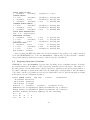
7
OUTPUT MESSAGE FILE: OUTFILE
Here, the description of the output messages is given. Also short introduction to the structure of the
program is described (see Figure 2).
Consider the output file made for NbC during the calculation of the dynamical matrix (RUNMODE=4) for the point q=(0,0,1). Running the program in other modes produces similar output.
7.1
Reading Input Data
The execution of the MAGPLW package (source file magmain.f) starts from reading the input data
controlled by INIT subroutine (see file init.f). Beginning of the OUTFILE contains the information
read from the INI/STRFILEs.
<<<--- INPUT INIFILE READ --->>>
*** Band Structure Calculation of bcc-Fe ***
--------------------------------------------------<CONTROL PARAMETERS>
:
lmto = 1
- Unscreened LMTO is on
lrwf = 1
- Adjust Phi to Veff only
npfr = 0
- Atomic forces
are off
<EXCHANGE-CORRELATION> :
ixc
=14
- Vosko-Wilk-Nussair + GGA91
<ATOMIC DATA>
:
natom = 1
- # of atoms in unit-cell
nsort = 1
- # of atoms of different type
par
= 5.425000
- lattice parameter in a.u.
nspin = 2
- including spin-polarization
norbs = 1
- without spin-orbit coupling
nkap = 3
- # of kappas in valence panel
Etail1= -.50000E-01
- Hankel tail energy
Etail2= -1.0000
- Hankel tail energy
Etail3= -2.5000
- Hankel tail energy
<OUTPUT DATA>
:
icon = 2
- read str. const. from INP/fe.con
iftr = 0
- no storage fourier con.
ibnd = 2
- save tetra.bands
in INP/fe.bnd
idos = 0
- no d.o.s.calculation
ipot = 0
- no storage of full potential
iscf = 1
- save full density
in INP/fe.scf
iout > 1
- print current output
<OTHER DATA>
:
nff
= 0
- # of bands below
EF
nef
= 9
- # of bands crossing EF
ndiv =16 16 16
- tetr.mesh for valence panel
ndic =32 32 32
- tetr.mesh for semicore panels
21
<ADDITIONAL INPUT FILES>:
ichub = 0
- with no Hubbard correction
ichop = 0
- with no hopping matrix
icopt = 0
- with no optical properties
icenr > 0
- with dense grid for int after INP/fe.enr
icpnt > 0
- with perturbation q’’s
after INP/fe.pnt
<<<--- INPUT LRTFILE READ --->>>
SET-UP DATA FOR LINEAR RESPONSE CALCULATIONS
--------------------------------------------------<GENERAL SETTINGS>
:
lift = 4
- Self-consistency is on
lplz = 0
- Polarizability
is off
lstn = 0
- Stoner matrix
is off
ldlf = 1
- Changes in phi are off
mode = 1
- Restart calcuation is off
<DEFAULT FILE SETTINGS>
:
iwgt = 1
- save tetra. weights in
WGT/wgt11w500
iphn = 0
- no storage of phonon modes
idsv = 0
- no storage of ind.potential
idro = 1
- update ind.density in
DRO/dro11g0w500m
idro = 1
- update psd.density in
DRO/dps11g0w500m
iout = 2
- save current output in
out11w500m
<<<--- INPUT STRFILE READ --->>>
****** Structure Data for bcc-Fe ******
--------------------------------------------------<CONTROL PARAMETERS>
:
natom = 1
- # of atoms in unit-cell
b/a
= 1.0000
- orthorombicity along b
c/a
= 1.0000
- orthorombicity along c
ibas = 1
- basis in Cartesian sys.
ibz
= 1
- automatic BZ - choice
icalc = 1
- using built-in calc.
istrn = 1
- distort cutoff sphere
ndiv1 = 4
- polyhedron
generation
ndiv2 = 1
- polyhedron surface grid
nvec = 300
- vectors in Evald method
alpha = 1.0000
- splitting factor there
<PRIMITIVE TRANSLATIONS> :
( -.50000
, .50000
, .50000
) ! R1x,R1y,R1z
( .50000
, -.50000
, .50000
) ! R2x,R2y,R2z
( .50000
, .50000
, -.50000
) ! R3x,R3y,R3z
22
<BASIS ATOMS IN CELL>
:
( .00000E+00, .00000E+00,
<STRAIN MATRIX>
:
( 1.0000
, .00000E+00,
( .00000E+00, 1.0000
,
( .00000E+00, .00000E+00,
<INVERSE STRAIN MATRIX> :
( 1.0000
, .00000E+00,
( .00000E+00, 1.0000
,
( .00000E+00, .00000E+00,
<POINT GROUP DESCRIPTION>:
ikov = C - Cubic system
<RECIPROCAL LATTICE>
:
( .00000E+00, 1.0000
,
( 1.0000
, .00000E+00,
( 1.0000
, 1.0000
,
<BRILLOUIN ZONE>
:
( .00000E+00, 1.0000
,
( 1.0000
, .00000E+00,
( 1.0000
, 1.0000
,
Cell Volume = 79.83057
.00000E+00) ! for Fe
.00000E+00) ! Sxx,Sxy,Sxz
.00000E+00) ! Syx,Syy,Syz
1.0000
) ! Szx,Szy,Szz
.00000E+00) ! Rxx,Rxy,Rxz
.00000E+00) ! Ryx,Ryy,Ryz
1.0000
) ! Rzx,Rzy,Rzz
1.0000
) ! G1x,G1y,G1z
1.0000
) ! G2x,G2y,G2z
.00000E+00) ! G3x,G3y,G3z
1.0000
) ! K1x,K1y,K1z
1.0000
) ! K2x,K2y,K2z
.00000E+00) ! K3x,K3y,K3z
After executing the INIT subrouitine, the execution transfers to the package of programs controlled
by module ELECTRONS (see source file electrons.f). This module prepares structure constants,
energy bands and wave functions necessary for linear–response calculations.
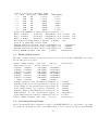
7.2
Preparing Structure Constants
STRMSH (see source file strmsh.f). prepares data depending on the crystalline structure. Next line
gives an information about number of the point group elements found for the lattice. The number of
k-points generated for the main valence panel (controlled by parameters nk1,nk2,nk3) (the number of
k–points for all semicore panels is the same as for the main valence panel) is printed. Also the number
of k–points controlled by parameters nw1,nw2,nw3 which will be used to find the integration weights
in the linear–response calculation is printed.
******* STRMSH started ; CPU time:
3.290000
************
48 elements discovered
145 k-points generated
897 k-points to weight
Position : ( .00000E+00, .00000E+00, .00000E+00) for Fe
LMTO-basis set is expanded in spherical harmonics up to Lmax= 6
Charge density is expanded in spherical harmonics up to Lmax= 6
Non-zero elements allowed by symmetry are the following:
l= 0 ; m=
0
l= 4 ; m=
-4
0
4
l= 6 ; m=
-4
0
4
23
Total # of non-zero components found
7
l=
Nplw
Ecut (Ry)
RH(S)/H(S)
GH(S)/RH(S)
’’ 0’’
2346
145.
1.00000
1.00000
’’ 1’’
2346
145.
1.00000
1.0000
’’ 2’’
2346
145.
.99999
1.0000
’’ 3’’
2346
145.
.99997
.99997
’’ 4’’
2346
145.
.99984
.99972
’’ 5’’
2346
145.
.99944
1.0001
’’ 6’’
2346
145.
.99833
1.0030
Result from VECGEN for direct/reciprocal spaces --->
Rmax= 2.616219
; Accuracy= .2938758E-23; # of vectors=
169
Gmax= 6.592308
; Accuracy= .1165861E-16; # of vectors=
603
Smax= 4.473601
; Accuracy= .2950956E-23; # of vectors=
749
Min.energy for using Evald’’s method= -4.983823
Ry
Total # of connecting vectors found
1
Minimum difference between |k+G|^2 and kappa1^2 is
.3727432E-01
Minimum difference between |k+G|^2 and kappa2^2 is
.7454864
Minimum difference between |k+G|^2 and kappa3^2 is
1.863716
******* STRMSH finished ; CPU time:
5.330000
************
7.3
Finding Full Potential
The full potential is calculated in the same way as it is done in the package NMTPLW. As a result,
the following table is produced.
******* VFULL started ; CPU time:
5.610000
************
Input data for Fe
in the position
1 ------->
V-up(S)= -.1249418
| RO-up(S)= .2056066E-01
P-up(S)= -.1063844
| PD-up(S)= .2023072E-01
P-up(0)= -13.07857
| PD-up(0)= .1934313E-02
V-dn(S)= -.1189130
| RO-dn(S)= .2110278E-01
P-dn(S)= -.1553160
| PD-dn(S)= .2074349E-01
P-dn(0)= -12.83667
| PD-dn(0)= .1148676E-02
M(S)= 2.257298
|
PM(S)= 1.115492
Average potential over the sphere boundaries is -.1219274
Average potential in the interstitial region is -.1917914E-01
Total charge in the interstitial region must be
.9574413
Total charge found via fourier transform is
.9574413
Auxilary density renormalization coefficient is
.9999995
Magnetization in the interstitial region is -.5352703E-01
Total magnetization found in elementary cell is
2.203771
******* VFULL finished ; CPU time:
60.10000
************
7.4
Calculating Energy Bands
After constructing the full potential the execution of the ELECTRONS goes to the package of program
for solving the eigenvalue problem of the LMTO method. It is controlled ba the program BANDS
24
(see source file bands.f). Information about choice of Eny is printed below.
******** BANDS started
3kappa spin-up panel #
Eny:
Dny:
.45655
-.31805
.60984
.51403
.65804
-1.3297
Eny:
Dny:
.45655
-.31805
.60984
.51403
.65804
-1.3297
Eny:
Dny:
.45655
-.31805
.60984
.51403
.65804
-1.3297
3kappa spin-dn panel #
Eny:
Dny:
.45655
-.31805
.60984
.51403
.65804
-1.3297
Eny:
Dny:
.45655
-.31805
.60984
.51403
.65804
-1.3297
Eny:
Dny:
.45655
-.31805
.60984
.51403
.65804
-1.3297
******** BANDS finished
7.5
; CPU time:
60.10000
************
1 : Band Structure Calculation of E(k) with :
Cny:
Wny:
Et= -.500E-01 for Fe
.84610
4.9488
for 4s-state, center
2.1312
1.9378
for 4p-state, center
.76716
.27252
for 3d-state, center
Cny:
Wny:
Et= -1.00
for Fe
.84610
4.9488
for 4s-state, center
2.1312
1.9378
for 4p-state, center
.76716
.27252
for 3d-state, center
Cny:
Wny:
Et= -2.50
for Fe
.84610
4.9488
for 4s-state, center
2.1312
1.9378
for 4p-state, center
.76716
.27252
for 3d-state, center
; CPU time:
63.59000
************
Integrating over Brillouin Zone
After the band structure calculation finished, the Brillouin zone integration starts (controlled by
BZINT, see source file bzint.f). The information below contains the Fermi energy found (EF), number
of states calculated (TOS) which must coincide with the total valence charge. DOS stands for the
density of states. Numbers of fully filled bands and the number of bands crossing the Fermi level
are for information only. They will not overwrite the input numbers nff, nef from the INIFILE. The
line ”LR-Information” contains a hint for choosing the parameters nff, nef in the linear–response
calculation. Another hint is: Locate the band nearest to the Fermi energy. Step out from this band by
approximately 0.5 Ry down. Count the bands below this energy, they can be treated as filled bands
nff. The bands located at the energy window plus/minus 0.5 Ry from the Fermi energy should be
treated as the bands crossing EF (nef). Note that this is only necessary for metals, use true number
of filled bands and set nef=0 for semiconductors. Also when calculating electron–phonon matrices,
use true number of the bands crossing the Fermi level, otherwise storage of the wave functions will be
exceedingly large.
25
******** BZINT started ; CPU time:
63.59000
************
EF,TOS,DOS==
.7928632
7.989166
14.10590
EF,TOS,DOS==
.7936313
7.999986
14.09788
EF,TOS,DOS==
.7936323
8.000000
14.09784
EF,TOS,DOS==
.7936323
8.000000
14.09784
Calculated average square of electron velocities:
<Vx^2>= .7472877
; <Vy^2>= .7472877
; <Vz^2>= .6956963
Calculated bare plasma frequencies (in eV):
om_p^x= 6.599383
; om_p^y= 6.599383
; om_p^z= 6.367504
# of fully filled bands =
2; input # =
0
# of bands crossing Ef =
4; input # =
9
Energy bands at the Gamma-point for spin-up states are
.18539
.63131
.63131
.63131
.71606
.71606
3.1184
3.1184
3.1184
3.1976
3.1976
3.8412
3.8412
3.8412
4.6837
5.6510
5.6510
5.6510
7.7848
7.8404
7.8404
12.028
12.028
12.028
12.315
12.315
12.315
Energy bands at the Gamma-point for spin-dn states are
.20076
.76970
.76970
.76970
.91505
.91505
3.1747
3.1747
3.1938
3.1938
3.1938
3.8547
3.8547
3.8547
4.6752
5.6774
5.6774
5.6774
7.8220
7.8220
7.8418
12.010
12.010
12.010
12.294
12.294
12.294
LR information: # of fully filled bands (nff) =
0
LR information: # of bands crossing EF (nef) =
6
******** BZINT finished ; CPU time:
290.1100
************
This is the end point for module ELECTRONS. Structure constants, energy bands and wave
functions are stored in CONFILE,BNDFILE, and PSIFILE and are ready for use as shareable files.
The execution tranfers to the module MAGNONS (see file magnons.f).
7.6
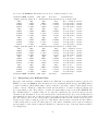
Preparing Integration Weights
The first step performed by the module MAGNONS is the calculation of the k–space integration
weights necessary for calculating induced charge density and magnetization. The information about
symmetry of the q vector is printed out. It includes number of equivalent operations (group) for this
vector, as well as its symmetry star.
******* CHITET started ; CPU time:
290.1100
************
Symmetry analysis for q = ( .0000E+00, .0000E+00, .7500
)
1) group of q-vector contains 8 elements
2) star of q-vector contains 6 elements
Calculated average square of electron velocities:
<Vx^2>= .7472877
; <Vy^2>= .7472877
; <Vz^2>= .6956963
26
Calculated bare plasma frequencies (in units
om_p^x= 6.599383
; om_p^y= 6.599383
UP-states: TEST,TOSK,DOSK==
1.000000
UP-states: TEST,TOSQ,DOSQ==
1.000000
DN-states: TEST,TOSK,DOSK==
1.000000
DN-states: TEST,TOSQ,DOSQ==
1.000000
AL-states: TEST,TOSK,DOSK==
2.000000
AL-states: TEST,TOSQ,DOSQ==
2.000000
eV):
; om_p^z=
2.551241
2.551241
1.448759
1.448759
4.000000
4.000000
6.367504
5.341420
5.341420
1.707500
1.707500
7.048919
7.048919
When the integration weights are calculated, the following test lines are printed out.
UP-states: TEST,TOSK,DOSK==
1.000000
2.551241
UP-states: TEST,TOSQ,DOSQ==
1.000000
2.551241
DN-states: TEST,TOSK,DOSK==
1.000000
1.448759
DN-states: TEST,TOSQ,DOSQ==
1.000000
1.448759
AL-states: TEST,TOSK,DOSK==
2.000000
4.000000
AL-states: TEST,TOSQ,DOSQ==
2.000000
4.000000
Susceptibility calculation, states UP-UP:
ibnd ibnd1
chi(V)
chi(F)
chi1(d)
1
1
.0000000E+00
.0000000E+00
.0000000E+00
1
2
.0000000E+00
.0000000E+00
.0000000E+00
1
3 -.9930953E-03
.0000000E+00 -.9516821E-03
1
4 -.2953428E-02
.0000000E+00 -.2827720E-02
1
5 -.3706024
.0000000E+00 -.3389146
1
6 -1.671572
.0000000E+00 -1.571990
1
7 -.9241452
.0000000E+00 -.9152159
truncated
5.341420
5.341420
1.707500
1.707500
7.048919
7.048919
chi2(d)
.0000000E+00
.0000000E+00
-.9002467E-03
-.2673846E-02
-.3126199
-1.466132
-.8849650
After the line ”DELSTR finished” is printed out, the integration weights are ready. They are
stored in WGTFILE placed in the WGT directory. Note that WGTFILE has a dependence on the
wave vector q but not on the displacement and polarization.
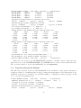
7.7
Calculating Induced Potential
After calculating integration weights and polarizabilities, the self–consistent cycle begins. As a first
step here, the potential induced by particular displacements and polarizations is calculated. This
is controlled by module DELPOT (see source file delpot.f). The values of the induced potential,
induced pseudopotential at the sphere boundary, as well as the values of the induced density and the
induced pseudodensity at the sphere boundary are printed out.
===========================================================================
ITERATION
1 FOR Q-VECTOR ( .0000E+00, .0000E+00, .7500
)
===========================================================================
******* DELPOT started ; CPU time:
7246.610
MAGNETIC FIELD POLARIZATION ’’m’’
G 0=( .00000E+00, .00000E+00, .00000E+00)
27
************
Data variation :: atom position 1 for Fe
Screened potential and magnetic fields ------->
Total potential Dpot(S) = ( .0000000E+00, .0000000E+00)
Pseudopotential Ppot(S) = ( .0000000E+00, .0000000E+00)
Z magnet. field DBm0(S) = ( .0000000E+00, .0000000E+00)
M magnet. filed DBm_(S) = ( .1449128E-02, .0000000E+00)
P magnet. field DBm+(S) = ( .0000000E+00, .0000000E+00)
Z magnet. field PBm0(S) = ( .0000000E+00, .0000000E+00)
M magnet. filed PBm_(S) = ( -.1049874E-01, .0000000E+00)
P magnet. field PBm+(S) = ( .0000000E+00, .0000000E+00)
Induced density and magnetization
------->
Induced density Drho(S) = ( .0000000E+00, .0000000E+00)
Pseudo density Prho(S) = ( .0000000E+00, .0000000E+00)
Z Magnetization DMg0(S) = ( .0000000E+00, .0000000E+00)
M Magnetization DMg_(S) = ( .0000000E+00, .0000000E+00)
P Magnetization DMg+(S) = ( .0000000E+00, .0000000E+00)
Z Pseudomagnetz PMg0(S) = ( .0000000E+00, .0000000E+00)
M Pseudomagentz PMg_(S) = ( .0000000E+00, .0000000E+00)
P Pseudomagentz PMg+(S) = ( .0000000E+00, .0000000E+00)
Induced charges and magnetic moments
------->
Induced charge in S_mt = ( .0000000E+00, .0000000E+00)
Pseudo charge in S_mt = ( .0000000E+00, .0000000E+00)
Z Magnetic moment Dmom0 = ( .0000000E+00, .0000000E+00)
M Magnetic moment Dmom_ = ( .0000000E+00, .0000000E+00)
P Magnetic moment Dmom+ = ( .0000000E+00, .0000000E+00)
******* DELPOT finished ; CPU time:
7418.510
*******
7.8
Calculating Induced Charge Density
After constructing induced potential, induced charge density is calculated. This part is controlled by
the module DELBND (source file delbnd.f). Changes in Eny which are induced by the perturbation
are printed out.
******* DELBND started ; CPU time:
7418.510
************
3kappa Panel # 1 :: Calculation of Linear Response ------->
MAGNETIC FIELD POLARIZATION ’’m’’
G 0=( .00000E+00, .00000E+00, .00000E+00)
Delta{Eny} :
Ekap= -.5000E-01 for Fe
( .0000000E+00, .0000000E+00) for 4s state
( .0000000E+00, .0000000E+00) for 4p state
( .0000000E+00, .0000000E+00) for 3d state
Delta{Eny} :
Ekap= -1.000
for Fe
( .0000000E+00, .0000000E+00) for 4s state
( .0000000E+00, .0000000E+00) for 4p state
( .0000000E+00, .0000000E+00) for 3d state
Delta{Eny} :
Ekap= -2.500
for Fe
28
( .0000000E+00, .0000000E+00) for 4s state
( .0000000E+00, .0000000E+00) for 4p state
( .0000000E+00, .0000000E+00) for 3d state
MAGNETIC FIELD POLARIZATION ’’m’’
G 0=( .00000E+00, .00000E+00, .00000E+00)
Delta{Eny} :
Ekap= -.5000E-01 for Fe
( .0000000E+00, .0000000E+00) for 4s state
( .0000000E+00, .0000000E+00) for 4p state
( .0000000E+00, .0000000E+00) for 3d state
Delta{Eny} :
Ekap= -1.000
for Fe
( .0000000E+00, .0000000E+00) for 4s state
( .0000000E+00, .0000000E+00) for 4p state
( .0000000E+00, .0000000E+00) for 3d state
Delta{Eny} :
Ekap= -2.500
for Fe
( .0000000E+00, .0000000E+00) for 4s state
( .0000000E+00, .0000000E+00) for 4p state
( .0000000E+00, .0000000E+00) for 3d state
******* DELBND finished ; CPU time:
8170.590
************
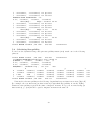
7.9
Calculating Susceptibility
To find out the dynamical charge and spin susceptibility matrix (4×4) watch out for the following
printout:
******* CHIMAT started ; CPU time:
8170.950
************
** COMPLEX SUSCEPTIBILITY Chi(q+G 0,g+G 0,omega) **
Q-VECTOR: ( .0000E+00, .0000E+00, .7500
)
G 0=( .00000E+00, .00000E+00, .00000E+00)
G 0=( .00000E+00, .00000E+00, .00000E+00)
FREQUENCY = .3674903E-01 Ry ;
500.0000
meV.
m
z
p
m
.0000E+00 .0000E+00| .0000E+00 .0000E+00| .0000E+00 .0000E+00|
z
.0000E+00 .0000E+00| .0000E+00 .0000E+00| .0000E+00 .0000E+00|
p
1.688
.1524
| .0000E+00 .0000E+00| .0000E+00 .0000E+00|
v
.0000E+00 .0000E+00| .0000E+00 .0000E+00| .0000E+00 .0000E+00|
******* CHIMAT finished ; CPU time:
8171.000
************
v
.0000E+00
.0000E+00
.0000E+00
.0000E+00
.0000
.0000
.0000
.0000
Units used for the susceptibility are the following: longitudinal response functions are in st./[Ry*cell].
For example, the non–interacting (at first iteration) longitudinal susceptibility is exactly N (EF ) .
Transverse susceptibility is given in the units of magnetic moment. For q,ω=0, non–interacting (at
first iteration) χ+− (0, 0) should be equal to magnetic moment in the unit cell.
29
8
PARAMETER FILE: PARAM.DAT
The dimensions inside the program are defined using PARAMETER statements. All parameter statments are collected in one file called PARAM.DAT and are included in every program using INCLUDE
statement. PARAM.DAT used by MAGASA/PLW program is very similar to the file PARAM.DAT
used by NMTASA/PLW programs. We therefore refer to the manual of the NMT* packages for
complete description. Here, only two differences between the two files will be pointed out.
8.1
Differences with the NMT package
One more parameter statement is added in PARAM.DAT file of the MAGASA/PLW packages compared to that file of the NMT* packages.
PARAMETER (NBNDMAX=15) ! MAX.NUMBER OF BANDS CROSSING EF
This parameter sets maximal number of bands allowed to cross the Fermi level. The input parameter nef cannot exceed this number. Do not set NBNDMAX to the large number (say maximum
possible number of bands is NDIMMAX) since it affects the core memory.
8.2
Estimation of the needed core memory
The storage of the core memory is taken by many arrays. For the configuration with 5-6 atoms per
unit cell, the needed core memory can be of the order 100 Mbyte. A very useful option is to link the
programs and to get a map-file. Under UNIX it is: xlf *.o -o main.exe -bloadmap:map. At the
end of the map file there is a total amount of core memory required by the program.
Disc space: significant disc storage is taken by the induced charge density files located in the DRO
directory. For dealing with the systems of 5-6 atoms per cell, a free disc space of the order several
Gbytes is desired.
30
9
ERROR MESSAGES
The description of the error messages in the program is supposed to be essentially extended in the
future. Below just a few useful hints is given. Generally, two kind of errors exist in the program:
warning messages (when the program does not terminate) and the error messages (when the program
terminates). Normally warning messages mean that the program can either correct the problem itself
or the problem is not important for the execution (like an advise to switch on scalar relativism when
atomic charge exceeds 21). The error messages always mean that the program can give a wrong result
if the input files will not be corrected.
9.1
Errors connected with PARAM.DAT
In all cases the program will terminate if any of the actual parameters exceeds the parameter in the
PARAM.DAT. Then standard error message occurs which states which of the parameters must be
increased.
9.2
Errors connected with input
Some input data can be easily checked (like the number of atoms which is read from different input
files). If there is a mismatch in the input, a corresponding message is printed and execution is
terminated.
31
10
10.1
USING MAGLIB LIBRARY
Program QPNT
This program is used to generate irreducible points in the Brillouin zone. No special configuring of the
program is required. Just compile contents of the directory /maglib/qpnt/, link object files and get
executable make.exe. The input files to the program are INIFILE and STRFILE. The input line also
contains three divisions nq1,nq2,nq3 necessary to construct the grid of wave vectors q. The output
is the number of irreducible q points generated (according to the point group) and the list of points
which can be stored in the output file (called PNTFILE). An additional option is provided to generate
the irreducible points with its minimal lenght. This means that among a set of all q + G-points (G
is a reciprocal lattice vector) the vector with minimal length will be picked out. This option must be
used when generating wave vectors q for linear–response calculation.
32
11
Acknowledgments
I greatly acknowledge Dr. Andrej Postnikov who has initiated writing of this manual. Part of the
developments has been done in collaboration with my brother Dr. Dmitrij Savrasov. Special thanks
to Prof. Ole Andersen and Dr. Ove Jepsen who are my LMTO teachers.
12
COPYRIGHT
These programs are a free software for scientific and/or educational purposes.
It is not allowed to redistribute them without prior written consent of the Copyright owners.
It is illegal to commercially distribute these programs as a whole or incorporate any part of it into
a commercial product.
References
[1] P. Hohenberg and W. Kohn, Phys. Rev. 136, B864 (1964).
[2] W. Kohn and L. J. Sham, Phys. Rev. 140, A1133 (1965).
[3] For a review, see, also , Theory of the Inhomogeneous Electron Gas, edited by S. Lundqvist and S.
H. March (Plenum, New York, 1983).
[4] E. K. U. Gross and W. Kohn, Phys. Rev. Lett (1985).
[5] S. Y. Savrasov, Phys. Rev. Lett. 69, 2819 (1992).
[6] S. Y. Savrasov, Phys. Rev. B 54, 16470 (1996).
[7] S. Y. Savrasov, D. Y. Svarasov and O. K. Andersen, Phys. Rev. Lett. 72, 372 (1994).
[8] S. Y. Savrasov and D. Y. Savrasov, Phys. Rev. B 54, 16487 (1996).
[9] S. Y. Savrasov, Phys. Rev. Lett. 81 2570 (1998).
33