Download National Instruments Xmath Interactive Control Design Module ICDM User's Manual

NI MATRIXx
TM
Xmath Interactive Control Design Module
TM
Xmath Interactive Control Design Module
April 2007
370754C-01
Support
Worldwide Technical Support and Product Information
ni.com
National Instruments Corporate Headquarters
11500 North Mopac Expressway
Austin, Texas 78759-3504
USA Tel: 512 683 0100
Worldwide Offices
Australia 1800 300 800, Austria 43 662 457990-0, Belgium 32 (0) 2 757 0020, Brazil 55 11 3262 3599,
Canada 800 433 3488, China 86 21 5050 9800, Czech Republic 420 224 235 774, Denmark 45 45 76 26 00,
Finland 385 (0) 9 725 72511, France 33 (0) 1 48 14 24 24, Germany 49 89 7413130, India 91 80 41190000,
Israel 972 3 6393737, Italy 39 02 413091, Japan 81 3 5472 2970, Korea 82 02 3451 3400,
Lebanon 961 (0) 1 33 28 28, Malaysia 1800 887710, Mexico 01 800 010 0793, Netherlands 31 (0) 348 433 466,
New Zealand 0800 553 322, Norway 47 (0) 66 90 76 60, Poland 48 22 3390150, Portugal 351 210 311 210,
Russia 7 495 783 6851, Singapore 1800 226 5886, Slovenia 386 3 425 42 00, South Africa 27 0 11 805 8197,
Spain 34 91 640 0085, Sweden 46 (0) 8 587 895 00, Switzerland 41 56 2005151, Taiwan 886 02 2377 2222,
Thailand 662 278 6777, Turkey 90 212 279 3031, United Kingdom 44 (0) 1635 523545
For further support information, refer to the Technical Support and Professional Services appendix. o comment
on National Instruments documentation, refer to the National Instruments Web site at ni.com/info and enter
the info code feedback.
© 2007 National Instruments Corporation. All rights reserved.
Important Information
Warranty
The media on which you receive National Instruments software are warranted not to fail to execute programming instructions, due to defects
in materials and workmanship, for a period of 90 days from date of shipment, as evidenced by receipts or other documentation. National
Instruments will, at its option, repair or replace software media that do not execute programming instructions if National Instruments receives
notice of such defects during the warranty period. National Instruments does not warrant that the operation of the software shall be
uninterrupted or error free.
A Return Material Authorization (RMA) number must be obtained from the factory and clearly marked on the outside of the package before any
equipment will be accepted for warranty work. National Instruments will pay the shipping costs of returning to the owner parts which are covered by
warranty.
National Instruments believes that the information in this document is accurate. The document has been carefully reviewed for technical accuracy. In
the event that technical or typographical errors exist, National Instruments reserves the right to make changes to subsequent editions of this document
without prior notice to holders of this edition. The reader should consult National Instruments if errors are suspected. In no event shall National
Instruments be liable for any damages arising out of or related to this document or the information contained in it.
EXCEPT AS SPECIFIED HEREIN, NATIONAL INSTRUMENTS MAKES NO WARRANTIES, EXPRESS OR IMPLIED, AND SPECIFICALLY DISCLAIMS ANY WARRANTY OF
MERCHANTABILITY OR FITNESS FOR A PARTICULAR PURPOSE. CUSTOMER’S RIGHT TO RECOVER DAMAGES CAUSED BY FAULT OR NEGLIGENCE ON THE PART OF NATIONAL
INSTRUMENTS SHALL BE LIMITED TO THE AMOUNT THERETOFORE PAID BY THE CUSTOMER. NATIONAL INSTRUMENTS WILL NOT BE LIABLE FOR DAMAGES RESULTING
FROM LOSS OF DATA, PROFITS, USE OF PRODUCTS, OR INCIDENTAL OR CONSEQUENTIAL DAMAGES, EVEN IF ADVISED OF THE POSSIBILITY THEREOF. This limitation of
the liability of National Instruments will apply regardless of the form of action, whether in contract or tort, including negligence. Any action against
National Instruments must be brought within one year after the cause of action accrues. National Instruments shall not be liable for any delay in
performance due to causes beyond its reasonable control. The warranty provided herein does not cover damages, defects, malfunctions, or service
failures caused by owner’s failure to follow the National Instruments installation, operation, or maintenance instructions; owner’s modification of the
product; owner’s abuse, misuse, or negligent acts; and power failure or surges, fire, flood, accident, actions of third parties, or other events outside
reasonable control.
Copyright
Under the copyright laws, this publication may not be reproduced or transmitted in any form, electronic or mechanical, including photocopying,
recording, storing in an information retrieval system, or translating, in whole or in part, without the prior written consent of National
Instruments Corporation.
National Instruments respects the intellectual property of others, and we ask our users to do the same. NI software is protected by copyright and other
intellectual property laws. Where NI software may be used to reproduce software or other materials belonging to others, you may use NI software only
to reproduce materials that you may reproduce in accordance with the terms of any applicable license or other legal restriction.
Trademarks
MATRIXx™, National Instruments™, NI™, ni.com™, and Xmath™ are trademarks of National Instruments Corporation. Refer to the Terms of
Use section on ni.com/legal for more information about National Instruments trademarks.
Other product and company names mentioned herein are trademarks or trade names of their respective companies.
Members of the National Instruments Alliance Partner Program are business entities independent from National Instruments and have no agency,
partnership, or joint-venture relationship with National Instruments.
Patents
For patents covering National Instruments products, refer to the appropriate location: Help»Patents in your software, the patents.txt file
on your CD, or ni.com/patents.
WARNING REGARDING USE OF NATIONAL INSTRUMENTS PRODUCTS
(1) NATIONAL INSTRUMENTS PRODUCTS ARE NOT DESIGNED WITH COMPONENTS AND TESTING FOR A LEVEL OF
RELIABILITY SUITABLE FOR USE IN OR IN CONNECTION WITH SURGICAL IMPLANTS OR AS CRITICAL COMPONENTS IN
ANY LIFE SUPPORT SYSTEMS WHOSE FAILURE TO PERFORM CAN REASONABLY BE EXPECTED TO CAUSE SIGNIFICANT
INJURY TO A HUMAN.
(2) IN ANY APPLICATION, INCLUDING THE ABOVE, RELIABILITY OF OPERATION OF THE SOFTWARE PRODUCTS CAN BE
IMPAIRED BY ADVERSE FACTORS, INCLUDING BUT NOT LIMITED TO FLUCTUATIONS IN ELECTRICAL POWER SUPPLY,
COMPUTER HARDWARE MALFUNCTIONS, COMPUTER OPERATING SYSTEM SOFTWARE FITNESS, FITNESS OF COMPILERS
AND DEVELOPMENT SOFTWARE USED TO DEVELOP AN APPLICATION, INSTALLATION ERRORS, SOFTWARE AND HARDWARE
COMPATIBILITY PROBLEMS, MALFUNCTIONS OR FAILURES OF ELECTRONIC MONITORING OR CONTROL DEVICES,
TRANSIENT FAILURES OF ELECTRONIC SYSTEMS (HARDWARE AND/OR SOFTWARE), UNANTICIPATED USES OR MISUSES, OR
ERRORS ON THE PART OF THE USER OR APPLICATIONS DESIGNER (ADVERSE FACTORS SUCH AS THESE ARE HEREAFTER
COLLECTIVELY TERMED “SYSTEM FAILURES”). ANY APPLICATION WHERE A SYSTEM FAILURE WOULD CREATE A RISK OF
HARM TO PROPERTY OR PERSONS (INCLUDING THE RISK OF BODILY INJURY AND DEATH) SHOULD NOT BE RELIANT SOLELY
UPON ONE FORM OF ELECTRONIC SYSTEM DUE TO THE RISK OF SYSTEM FAILURE. TO AVOID DAMAGE, INJURY, OR DEATH,
THE USER OR APPLICATION DESIGNER MUST TAKE REASONABLY PRUDENT STEPS TO PROTECT AGAINST SYSTEM FAILURES,
INCLUDING BUT NOT LIMITED TO BACK-UP OR SHUT DOWN MECHANISMS. BECAUSE EACH END-USER SYSTEM IS
CUSTOMIZED AND DIFFERS FROM NATIONAL INSTRUMENTS' TESTING PLATFORMS AND BECAUSE A USER OR APPLICATION
DESIGNER MAY USE NATIONAL INSTRUMENTS PRODUCTS IN COMBINATION WITH OTHER PRODUCTS IN A MANNER NOT
EVALUATED OR CONTEMPLATED BY NATIONAL INSTRUMENTS, THE USER OR APPLICATION DESIGNER IS ULTIMATELY
RESPONSIBLE FOR VERIFYING AND VALIDATING THE SUITABILITY OF NATIONAL INSTRUMENTS PRODUCTS WHENEVER
NATIONAL INSTRUMENTS PRODUCTS ARE INCORPORATED IN A SYSTEM OR APPLICATION, INCLUDING, WITHOUT
LIMITATION, THE APPROPRIATE DESIGN, PROCESS AND SAFETY LEVEL OF SUCH SYSTEM OR APPLICATION.
Conventions
The following conventions are used in this manual:
»
The » symbol leads you through nested menu items and dialog box options
to a final action. The sequence File»Page Setup»Options directs you to
pull down the File menu, select the Page Setup item, and select Options
from the last dialog box.
This icon denotes a note, which alerts you to important information.
bold
Bold text denotes items that you must select or click in the software, such
as menu items and dialog box options. Bold text also denotes parameter
names.
italic
Italic text denotes variables, emphasis, a cross-reference, or an introduction
to a key concept. Italic text also denotes text that is a placeholder for a word
or value that you must supply.
monospace
Text in this font denotes text or characters that you should enter from the
keyboard, sections of code, programming examples, and syntax examples.
This font is also used for the proper names of disk drives, paths, directories,
programs, subprograms, subroutines, device names, functions, operations,
variables, filenames, and extensions.
monospace bold
Bold text in this font denotes the messages and responses that the computer
automatically prints to the screen. This font also emphasizes lines of code
that are different from the other examples.
monospace italic
Italic text in this font denotes text that is a placeholder for a word or value
that you must supply.
Contents
Chapter 1
Introduction
Using This Manual.........................................................................................................1-1
Document Organization...................................................................................1-1
Commonly-Used Nomenclature......................................................................1-3
Related Publications ........................................................................................1-3
MATRIXx Help...............................................................................................1-4
ICDM Overview ............................................................................................................1-4
SISO Versus MIMO Design............................................................................1-4
Starting ICDM .................................................................................................1-4
Chapter 2
Introduction to SISO Design
SISO Design Overview..................................................................................................2-1
Basic SISO Terminology.................................................................................2-1
Overview of ICDM .......................................................................................................2-3
ICDM Windows ..............................................................................................2-3
ICDM Main Window ........................................................................2-4
PID Synthesis Window .....................................................................2-4
Root Locus Synthesis Window .........................................................2-4
Pole Place Synthesis Window...........................................................2-4
LQG Synthesis Window ...................................................................2-5
H-Infinity Synthesis Window ...........................................................2-5
History Window................................................................................2-5
Alternate Plant Window....................................................................2-5
Key Transfer Functions and Data Flow in ICDM ...........................................2-5
Summary ...........................................................................................2-6
Origin of the Controller.....................................................................2-6
What the ICDM Main Window Plots Show .....................................2-7
Controller/Synthesis Window Compatibilities................................................2-7
Using ICDM ....................................................................................................2-9
General Plotting Features ................................................................................2-11
Ranges of Plots and Sliders...............................................................2-11
Zooming ............................................................................................2-12
Data-Viewing Plots ...........................................................................2-12
Interactive Plot Re-ranging ...............................................................2-13
© National Instruments Corporation
v
Xmath Interactive Control Design Module
Contents
Graphically Manipulating Poles and Zeros..................................................... 2-13
Editing Poles and Zeros .................................................................... 2-13
Editing Poles and Zeros Graphically .............................................................. 2-14
Complex Poles and Zeros ................................................................. 2-14
Isolated Real Poles and Zeros........................................................... 2-14
Nonisolated Real Poles and Zeros and Almost Real Pairs ............... 2-14
Adding/Deleting Poles and Zeros..................................................... 2-15
Adding/Deleting Pole-Zero Pairs ..................................................... 2-15
Chapter 3
ICDM Main Window
Window Anatomy ......................................................................................................... 3-1
Communicating with Xmath ........................................................................... 3-2
Most Common Usage ....................................................................... 3-3
Default Plants ................................................................................... 3-3
Saving and Restoring an ICDM Session .......................................... 3-3
Reading Another Plant into ICDM ................................................... 3-3
Reading a Controller from Xmath into ICDM ................................. 3-4
Writing the Plant Back to Xmath ..................................................... 3-4
Writing the Alternate Plant back to Xmath ...................................... 3-4
Writing a Controller on the History List to Xmath .......................... 3-4
ICDM Plots ..................................................................................................... 3-5
Selecting Plots................................................................................................. 3-5
Ranges of Plots ................................................................................. 3-6
Plot Magnify Windows..................................................................... 3-7
Selecting a Synthesis or History Window ..................................................................... 3-9
Edit Menu ...................................................................................................................... 3-9
Chapter 4
PID Synthesis
Window Anatomy ......................................................................................................... 4-1
PID Controller Terms .................................................................................................... 4-1
Toggling Controller Terms On and Off .......................................................... 4-2
Opening the PID Synthesis Window .............................................................. 4-4
Manipulating the Controller Parameters ....................................................................... 4-4
Time Versus Frequency Parameters ............................................................... 4-5
Ranges of Sliders and Plots............................................................................. 4-5
Controller Term Normalizations ..................................................................... 4-5
Integral Term Normalization ............................................................ 4-5
Derivative Term Normalization........................................................ 4-6
Rolloff Term Normalization ............................................................. 4-6
Xmath Interactive Control Design Module
vi
ni.com
Contents
Chapter 5
Root Locus Synthesis
Overview........................................................................................................................5-1
Window Anatomy..........................................................................................................5-1
Opening the Root Locus Synthesis Window .................................................................5-3
Terminology...................................................................................................................5-3
Plotting Styles ................................................................................................................5-4
Phase Contours ................................................................................................5-5
Magnitude Contours ........................................................................................5-5
Slider and Plot Ranges.....................................................................................5-6
Manipulating the Parameters .........................................................................................5-6
Design ............................................................................................................................5-7
Adding a Pole-Zero Pair..................................................................................5-7
Deleting Pole-Zero Pairs .................................................................................5-7
Interpreting the Nonstandard Contour Plots....................................................5-8
Chapter 6
Pole Place Synthesis
Window Anatomy..........................................................................................................6-1
Pole Place Modes...........................................................................................................6-2
Normal Mode...................................................................................................6-3
Integral Action Mode ......................................................................................6-4
State-Space Interpretation ...............................................................................6-5
Opening the Pole Place Window.....................................................................6-5
Manipulating the Closed-Loop Poles ............................................................................6-5
Time and Frequency Scaling ...........................................................................6-5
Butterworth Configuration ..............................................................................6-6
Editing the Closed-Loop Poles........................................................................6-6
Slider and Plot Ranges.....................................................................................6-6
Chapter 7
LQG Synthesis
LQG Synthesis Window Anatomy ................................................................................7-1
Synthesis Modes ............................................................................................................7-3
Opening the LQG Synthesis Window .............................................................7-3
Setup and Terminology ...................................................................................7-4
Standard LQG (All Toggle Buttons Off).........................................................7-4
Integral Action.................................................................................................7-5
Exponential Time Weighting ..........................................................................7-5
Output Weight Editing ....................................................................................7-6
State-Space Interpretation ...............................................................................7-7
© National Instruments Corporation
vii
Xmath Interactive Control Design Module
Contents
Manipulating the Design Parameters............................................................................. 7-7
Manipulating the Design Parameters Graphically .......................................... 7-7
Ranges ............................................................................................................. 7-8
Chapter 8
H-Infinity Synthesis
H-Infinity Synthesis Window Anatomy........................................................................ 8-1
Opening the Synthesis Window .................................................................................... 8-3
Setup and Synthesis Method ......................................................................................... 8-3
Central H-Infinity Controller .......................................................................... 8-4
Output Weight Editing .................................................................................... 8-5
Manipulating the Design Parameters............................................................................. 8-6
Manipulating the Weight Transfer Function................................................... 8-6
Infeasible Parameter Values............................................................................ 8-6
Ranges ............................................................................................................. 8-7
Chapter 9
History Window
Saving the Current Controller on the History List ........................................................ 9-1
Opening the History Window........................................................................................ 9-1
History Window Anatomy ............................................................................................ 9-1
Selecting the Active Controller ..................................................................................... 9-2
Editing the Comments ................................................................................................... 9-2
Deleting History List Entries......................................................................................... 9-3
To Continue Designing from a Saved Controller.......................................................... 9-3
Cycling Through Designs.............................................................................................. 9-3
Writing a Saved Design to Xmath................................................................................ 9-3
Using the History List ................................................................................................... 9-4
Chapter 10
Alternate Plant Window
Role and Use of Plant and Alternate Plant .................................................................... 10-1
Displaying the Alternate Plant Responses..................................................................... 10-1
Alternate Plant Window Anatomy ................................................................................ 10-2
Opening the Alternate Plant Window............................................................................ 10-3
Normalization ................................................................................................................ 10-4
Manipulating the Parameters......................................................................................... 10-4
Using the Alternate Plant Window................................................................................ 10-5
Robustness to Plant Variations ....................................................................... 10-5
Adding Unmodeled Dynamics........................................................................ 10-5
Ranges of Sliders and Plot .............................................................................. 10-6
Xmath Interactive Control Design Module
viii
ni.com
Contents
Chapter 11
Introduction to MIMO Design
Basic Terminology for MIMO Systems ........................................................................11-1
Feedback System Configuration......................................................................11-1
Transfer Functions .........................................................................................................11-2
Integral Action.................................................................................................11-4
Overview of ICDM for MIMO Design..........................................................................11-5
ICDM MIMO Windows ..................................................................................11-5
Main Window..................................................................................................11-5
MIMO Plot Window........................................................................................11-6
History Window ..............................................................................................11-7
Alternate Plant Window (MIMO Version)......................................................11-7
Chapter 12
LQG/H-Infinity Synthesis
Window Anatomy..........................................................................................................12-1
LQG/H-Infinity Main Window .......................................................................12-1
LQG/H-Infinity Weights Window ..................................................................12-2
Decay Rate Window........................................................................................12-5
H-Infinity Performance Window.....................................................................12-5
Frequency Weights Window ...........................................................................12-6
Synthesis Modes and Window Usage............................................................................12-7
Opening the LQG/H-Infinity Synthesis Window............................................12-8
Setup and Terminology ...................................................................................12-8
Standard LQG (All Toggle Buttons “Off”) .....................................................12-11
Integral Action.................................................................................................12-11
Exponential Time Weighting ..........................................................................12-12
Weight Editing.................................................................................................12-12
How to Select w, u, y, and z.............................................................................12-13
H-Infinity Solution ..........................................................................................12-14
Manipulating the Design Parameters .............................................................................12-16
Main Window..................................................................................................12-16
Ranges .............................................................................................................12-17
© National Instruments Corporation
ix
Xmath Interactive Control Design Module
Contents
Chapter 13
Multi-Loop Synthesis
Multi-Loop Window Anatomy...................................................................................... 13-1
Setup and Synthesis Method ......................................................................................... 13-3
Multi-Loop Versus Multivariable Design....................................................... 13-3
Opening the Multi-Loop Synthesis Window .................................................. 13-7
Designing a Multi-Loop Controller............................................................................... 13-7
Graphical Editor .............................................................................................. 13-7
Selecting and Deselecting Loops .................................................................... 13-7
Editing and Deleting Loops ............................................................................ 13-8
Loop Gain Magnitude and Phase .................................................................... 13-8
Appendix A
Using an Xmath GUI Tool
Appendix B
Technical Support and Professional Services
Index
Xmath Interactive Control Design Module
x
ni.com
1
Introduction
The Xmath Interactive Control Design Module (ICDM) is a complete
library of classical and modern interactive control design functions that
takes full advantage of Xmath’s powerful, object-oriented, graphical
environment. It provides a flexible, intuitive interactive control design
framework. This manual provides an overview of different aspects of linear
systems analysis, describes the Xmath Interactive Control Design function
library, and gives examples of how you can use Xmath to solve problems
rapidly.
Using This Manual
This manual is meant to complement the Xmath Help system. The Xmath
Help system can be used to find answers to specific questions such as, “In
the Root Locus window, how can I add a new pair of complex poles to the
controller?” In contrast, this manual is intended for describing the general
concepts and operation of the ICDM.
Document Organization
This manual includes the following chapters:
•
Chapter 1, Introduction, starts with an outline of the manual and some
use notes. It also contains an overview of the Interactive Control
Design Module.
•
Chapter 2, Introduction to SISO Design, outlines the types of linear
systems the system object represents and then discusses the
implementation of a system within Xmath.
•
Chapter 3, ICDM Main Window, describes the use of the ICDM Main
Window, which includes communication with Xmath, displaying
warning and log messages, displaying a variety of standard plots,
selecting a synthesis method for controller design, and controlling
auxiliary windows.
•
Chapter 4, PID Synthesis, discusses the PID synthesis window. This
window is used to synthesize various types of standard classical SISO
controllers such as P, PI, PD, PID, lead-lag, and lag-lead.
© National Instruments Corporation
1-1
Xmath Interactive Control Design Module
Chapter 1
Introduction
•
Chapter 5, Root Locus Synthesis, describes the user interface,
terminology, and parameters used for root locus synthesis.
•
Chapter 6, Pole Place Synthesis, discusses the Pole Place synthesis
window, which is used to design a SISO controller by assigning the
closed-loop poles.
•
Chapter 7, LQG Synthesis, discusses the LQG synthesis window
which is used to synthesize a linear quadratic Gaussian (LQG)
controller for a SISO plant.
•
Chapter 8, H-Infinity Synthesis, describes the H∞ synthesis window
used for SISO plants. The H∞ synthesis window is used to synthesize
a central controller. Such controllers are sometimes called linear
exponential quadratic Gaussian (LEQG) or minimum entropy
controllers.
•
Chapter 9, History Window, describes the History window used for
SISO plants. The History window is used to display and manipulate the
design history list, which is a list of controllers that have been
explicitly saved during the design process.
•
Chapter 10, Alternate Plant Window, describes the form of the
Alternate Plant window used for SISO design.
•
Chapter 11, Introduction to MIMO Design, provides an introduction
to MIMO design building on the earlier discussions of SISO design.
ICDM automatically switches between SISO and MIMO modes
depending on the plant that is read in.
•
Chapter 12, LQG/H-Infinity Synthesis, describes the MIMO LQG/H∞
synthesis window. The LQG/H∞ window is used to synthesize both
LQG and H∞ controllers. The two design methods have been
combined in a single window because of the similarity regarding the
use of weights: constant weights, frequency-dependent weights, and
integrators.
•
Chapter 13, Multi-Loop Synthesis, describes multi-loop synthesis. The
multi-loop window is used to synthesize a MIMO controller using PID
and Root Locus methods, applying them one loop at a time. In many
practical industrial applications, this is the way control systems are
designed for complex multivariable plants.
•
Appendix A, Using an Xmath GUI Tool, describes the basics of using
an Xmath GUI tool. Throughout this manual, extended examples
following each function discussion help pinpoint the flexibility and
applicability of the Interactive Control Design function library. This
appendix describes the basics of using an Xmath GUI tool.
Xmath Interactive Control Design Module
1-2
ni.com
Chapter 1
Introduction
Commonly-Used Nomenclature
This manual uses the following general nomenclature:
•
Matrix variables are generally denoted with capital letters; vectors are
represented in lowercase.
•
G(s) is used to denote a transfer function of a system where s is the
Laplace variable. G(q) is used when both continuous and discrete
systems are allowed.
•
H(s) is used to denote the frequency response, over some range of
frequencies of a system where s is the Laplace variable. H(q) is used to
indicate that the system can be continuous or discrete.
•
A single apostrophe following a matrix variable, for example, x',
denotes the transpose of that variable. An asterisk following a matrix
variable (for example, A*) indicates the complex conjugate, or
Hermitian, transpose of that variable.
Related Publications
For a complete list of MATRIXx publications, refer to Chapter 2,
MATRIXx Publications, Help, and Customer Support, of the MATRIXx
Getting Started Guide. The following documents are particularly useful for
topics covered in this manual:
•
MATRIXx Getting Started Guide
•
Xmath User Guide
•
Xmath Control Design Module
•
Xmath Interactive Control Design Module
•
Xmath Interactive System Identification Module, Part 1
•
Xmath Interactive System Identification Module, Part 2
•
Xmath Module Reduction Module
•
Xmath Optimization Module
•
Xmath Robust Control Module
•
Xmath Xμ Module
© National Instruments Corporation
1-3
Xmath Interactive Control Design Module
Chapter 1
Introduction
MATRIXx Help
Interactive Control Design Module function reference information
is available in the MATRIXx Help. The MATRIXx Help includes all
Interactive Control Design functions. Each topic explains a function’s
inputs, outputs, and keywords in detail. Refer to Chapter 2, MATRIXx
Publications, Help, and Customer Support, of the MATRIXx Getting
Started Guide for complete instructions on using the MATRIXx Help
feature.
ICDM Overview
This section provides an overview of the Interactive Control Design
Module, a tool for interactive design of continuous-time linear
time-invariant controllers. ICDM runs under Xmath, using the Xmath
Graphical User Interface (GUI).
SISO Versus MIMO Design
Version 2.0 of ICDM handles full multivariable design, that is, design of
multi-input multi-output (MIMO) controllers for MIMO plants. Thus
ICDM 2.0 operates in two basic modes: SISO design (single input, single
output) and MIMO design. The mode is determined automatically by the
plant you read into ICDM. The two different modes feature somewhat
different plot options, different synthesis options, and so on.
NI has made the notation, conventions, and windows used for MIMO
design as similar as possible to those used for SISO design. Therefore a
user familiar with version 1.0 of ICDM (which handled only SISO design)
should have little trouble using the new MIMO synthesis tools. NI also
recommends that the user who wishes to use ICDM for MIMO design start
by becoming familiar with its features for SISO design.
Chapters 2 through 10 discuss SISO design. Chapters 11 through 13 discuss
MIMO design. The MIMO descriptions have been written for the user who
is familiar with SISO design features.
Starting ICDM
To use ICDM, you should:
•
Have a user’s understanding of Microsoft Windows or X Windows and
the window manager that you use. For example, you should be able to
move, resize, and iconify windows; use a pull-down menu; and use a
scrollbar.
Xmath Interactive Control Design Module
1-4
ni.com
Chapter 1
Introduction
•
Have a user’s understanding of Xmath (enough to create a plant
transfer function).
•
Know the basics of how to interact with an Xmath GUI
application—for example, using a slider to set a parameter value, a
variable-edit box for typing in values, data-viewing, and plot zooming.
•
Know the basics of classical control system design (for SISO design)
and state-space design (for MIMO design).
An introduction to Xmath and a basic introduction to X Windows can be
found in the Xmath User Guide. There are several ways you can find out
about the basics of interacting with an Xmath GUI application:
•
Refer to Appendix A, Using an Xmath GUI Tool.
•
Enter guidemo in the Xmath Command window to start up the GUI
demo applications; this allows you to try out sliders, push buttons,
scrollbars, data-viewing, and so on.
After you have mastered the basic mechanics of using an Xmath GUI
application, you should be ready to get started.
To start up ICDM, enter icdm in the Xmath Command window:
Your window manager may require you to position a window that is created
using the left or middle mouse button. After the ICDM Main Window
appears, the Xmath command prompt will return. You now can use Xmath
and ICDM simultaneously.
The user interface for ICDM is designed to be intuitive; that is, things
mostly work the way you would assume that they should work, so you
should be able to start using ICDM immediately. NI recommends that you
read Chapter 2, Introduction to SISO Design, before using the module.
ICDM includes a complete Help system. In the menu bar of every ICDM
window there is a Help menu. The Help messages contain detailed
descriptions of every feature and function of ICDM. You can get a good
overview of the features of ICDM by scanning the entries in the menu bars
and reading the Help messages in the various windows.
ICDM function reference material is available in the MATRIXx Help. Refer
to Chapter 2, MATRIXx Publications, Help, and Customer Support, of the
MATRIXx Getting Started Guide for additional instructions on using the
MATRIXx Help.
© National Instruments Corporation
1-5
Xmath Interactive Control Design Module
2
Introduction to SISO Design
Xmath provides a structure for system representation called a system
object. This object includes system parameters in a data structure designed
to reflect the way these systems are analyzed mathematically. Operations
on these systems are likewise defined using operators that mirror as closely
as possible the notation control engineers use. This chapter outlines the
types of linear systems the system object represents and then discusses the
implementation of a system within Xmath. The functions used to create a
system object and to extract data from this object are an intrinsic part of the
object class and are also described. Finally, this chapter discusses the
functions check, discretize, and makecontinuous, which use information
stored in the system object to convert systems from one particular
representation to another.
SISO Design Overview
This section provides an overview of what ICDM does and how it works,
restricting the discussion to SISO design. If your interest is MIMO design,
you first should read this chapter and then Chapter 11, Introduction to
MIMO Design.
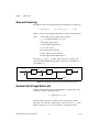
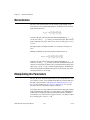
Basic SISO Terminology
This section describes the basic terminology and notation for SISO plants
and controllers used in ICDM and this manual. ICDM uses the standard
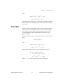
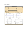
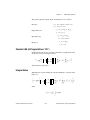
classical feedback configuration shown in Figure 2-1.
e
r
u
+
C(s)
y
P(s)
–
Figure 2-1. Standard Classical Feedback Configuration Used in ICDM
© National Instruments Corporation
2-1
Xmath Interactive Control Design Module
Chapter 2
Introduction to SISO Design
The equations describing this system are as follows:
y = Pu
u = Ce
e = r–y
where
y denotes the plant output or sensor signal
u denotes the plant input or actuator signal
r denotes the reference or command input signal
e denotes the error signal
P denotes the plant transfer function
C denotes the controller transfer function
In ICDM, the plant and controller transfer function are required to be
rational, that is, the ratio of two polynomials:
n p(s)
P(s) = ---------d p(s)
n c(s)
C(s) = ---------d c(s)
where np, dp, nc, and dc are polynomials called the plant numerator,
plant denominator, controller numerator, and controller denominator,
respectively. The symbols n and d are mnemonics for numerator and
denominator. The degree of dp is the plant order or plant degree. Similarly,
the degree of dc is the controller order or controller degree.
The poles and zeros of these transfer functions are the zeros (roots) of the
denominator and numerator polynomials, respectively.
In ICDM, P and C are required to be proper polynomials; that is, they have
at least as many poles as zeros. In other words, the degree of np is less than
or equal to the degree of dp (which is N) and similarly for nc and dc. In some
situations, the plant and controller are required to be strictly proper, which
means that there are more poles than zeros.
Other important terms include:
•
The loop transfer function L is defined as L = PC. The loop gain is the
magnitude of the loop transfer function.
•
The sensitivity transfer function is denoted as S and given by
S = 1/(1 + PC). The sensitivity transfer function is the transfer function
from the reference input r to the error signal e.
Xmath Interactive Control Design Module
2-2
ni.com
Chapter 2
Introduction to SISO Design
•
The closed-loop transfer function T is given by T = PC/(1 + PC). T is
the transfer function from r to y.
•
The characteristic polynomial of the system is defined as
X = nc np + dc dp. Its degree is equal to the order of the plant
plus the order of the controller.
•
The closed-loop poles are the zeros of the characteristic polynomial.
This definition avoids any problem with unstable pole-zero
cancellations between the plant and controller. The closed-loop zeros
are the zeros of nc np.
•
The output response to a unit step input (or just, the step response),
is the step response of the transfer function T; that is, the response of
y when the command input r is a unit step.
•
The actuator step response is the step response of the transfer function
C/(1 + PC), which is the transfer function from r to u.
•
Integral action means that the controller C has a pole at s = 0. Roughly
speaking, this means that the loop gain is very large at low frequencies.
Integral action implies that S(0) = 0, so if r is constant, the error e
converges to zero, that is, the output y(t) approaches r as t → ∞.
Overview of ICDM
This section provides a broad overview of the architecture, concepts, and
major functions of ICDM, restricting our discussion to the case of SISO
plants and controllers. This section also provides a summary of how ICDM
works and what it does.
ICDM Windows
ICDM supports many windows that serve a variety of functions. The most
important windows are:
•
ICDM Main window
•
PID Synthesis window
•
Root Locus Synthesis window
•
Pole Place Synthesis window
•
LQG Synthesis window
•
H∞ Synthesis window
•
History window
•
Alternate Plant window
© National Instruments Corporation
2-3
Xmath Interactive Control Design Module
Chapter 2
Introduction to SISO Design
These are briefly described in the following sections, and in more detail in
later chapters. Several of these windows have different forms for SISO and
MIMO design. This chapter restricts the discussion to the SISO forms.
Refer to Chapter 11, Introduction to MIMO Design, for a discussion of the
MIMO forms.
ICDM Main Window
The most important window is the ICDM Main window, which is used to:
•
Communicate with Xmath (for example, transfer plants/controllers
from/to Xmath).
•
Display warning and log messages.
•
Display a variety of standard plots.
•
Select a synthesis method for controller design.
•
Control several auxiliary windows.
PID Synthesis Window
The PID Synthesis window is used to synthesize a PID controller, with up
to two additional poles (usually used for high frequency rolloff). Each term
can be separately toggled on and off, so the PID window can be used to
synthesize P, PD, PI, PID, lead-lag, and lag-lead controllers. The design
parameters can be typed in, manipulated graphically by slider controls, or
manipulated graphically on a Bode plot of the controller transfer function.
Root Locus Synthesis Window
The Root Locus window can be used in many ways for synthesis and
analysis of controllers. It can display a conventional root locus in near
real-time, while the user drags controller poles and zeros. The user can
graphically create or destroy controller poles and zeros. The closed-loop
poles can be dragged along the root locus plot, which causes the gain
parameter to be set automatically. Nonconventional phase and gain
contours can be plotted as an aid to controller synthesis or robustness
analysis.
Pole Place Synthesis Window
The Pole Place Synthesis window is used to design a controller by
assigning the closed-loop poles. The closed-loop poles can be typed in, or
dragged on a plot. The closed-loop poles can be scaled in frequency or time
by graphical input, or assigned to a Butterworth configuration. The pole
place window supports integral action as an option.
Xmath Interactive Control Design Module
2-4
ni.com
Chapter 2
Introduction to SISO Design
LQG Synthesis Window
The LQG Synthesis window synthesizes LQG controllers, and therefore
can be used only with strictly proper plants. The user can vary weights for
the ratio of control (input) to regulation (output) cost and the ratio of sensor
(output) noise power to process (input) noise power. Optionally, the user
can specify a guaranteed decay rate and integral time constant. By dragging
zeros on a symmetric root locus plot, the user can vary the state weighting
or perform LTR design.
There also is a MIMO LQG window, described in Chapter 12,
LQG/H-Infinity Synthesis.
H-Infinity Synthesis Window
The H∞ Synthesis window synthesizes central H∞ controllers (also called
minimum entropy, risk sensitive, or LEQG controllers). The user can vary
weights for the ratio of control (input) to regulation (output) cost, the ratio
of sensor (output) noise power to process (input) noise power, and the risk
sensitivity or H∞ bound parameter γ. The user can vary the state weighting,
or equivalently, the output weight transfer function, by dragging zeros.
History Window
The History window is used to display and manipulate the design history
list, which is a list of controllers that have been explicitly saved during the
design process. The History window can be used to rapidly cycle through
and compare a subset of the saved designs. Any controller on the history
list can be recalled, and the design process continued.
Alternate Plant Window
The Alternate Plant window is used to study the robustness of a controller
to variations or changes in the plant. The user can interactively vary the
plant gain or dynamics, or add extra parasitic dynamics to the plant, see the
effect on the closed-loop system, and compare it to the nominal system.
Key Transfer Functions and Data Flow in ICDM
ICDM has three key transfer functions:
•
The plant transfer function P
•
The alternate plant transfer function Palt
•
The current controller transfer function C
© National Instruments Corporation
2-5
Xmath Interactive Control Design Module
Chapter 2
Introduction to SISO Design
The plant and the alternate plant have very different uses in ICDM, and
therefore different data flow characteristics.
The plant transfer function is read from Xmath into the ICDM Main
window, and is then exported to the synthesis windows that need it—Pole
Place, LQG, and H∞. In other words, the controllers designed using the
Pole Place, LQG, or H∞ Synthesis windows are based on the plant transfer
function. You cannot change the plant transfer function in ICDM except by
reading in a new plant from Xmath.
The alternate plant transfer function can be read into ICDM from Xmath,
or set equal to the plant transfer function. Its properties are very different
from the plant transfer function, however:
•
Using the Alternate Plant window, the user can graphically manipulate
the alternate plant transfer function.
•
The alternate plant transfer function is never exported to—that is, used
by—the synthesis windows that need to know the plant: Pole Place,
LQG, H∞.
The alternate plant transfer function is used to verify a controller design
that was based on the plant transfer function. The alternate plant transfer
function is used only to show the alternate plant plots in the ICDM Main
window. Refer to the What the ICDM Main Window Plots Show section.
Summary
The plant transfer function is used for design; the alternate plant transfer
function is used for (robustness) analysis or validation.
The distinction is not so important for PID and root locus design, because
the controller does not depend on the plant.
Origin of the Controller
The controller can originate from—that is, be designed by—several
possible sources:
•
An Open Synthesis window—For example, if the Pole Place Synthesis
window is open, then the current controller is determined by the Pole
Place Synthesis window. When you interact with the Pole Place
window by dragging a closed-loop pole to a new location, you will
be changing the current controller transfer function C.
•
The History window—If the History window is open, the controller
comes from the list of controllers that have been saved on the history
Xmath Interactive Control Design Module
2-6
ni.com
Chapter 2
Introduction to SISO Design
list. The current controller is the active or selected entry on the list of
saved controllers.
Only one synthesis window, or the History window, is allowed to be open
at any given time, which eliminates any possible confusion over the source
of the current controller. Remember the simple rule: If any synthesis
window, or the History window, is open, it is the source of the current
controller.
What the ICDM Main Window Plots Show
The plots in the ICDM Main window always use the plant and the current
controller. For example, the step response plot shows the step response of
the closed-loop system formed by the plant transfer function and the
current controller transfer function.
Optionally, the plots also can show the response of the alternate plant
connected with the current controller. In this case, the responses with the
plant and the alternate plant are shown in different line types or colors, and
can always be distinguished by data-viewing. Refer to the Data-Viewing
Plots section.
Controller/Synthesis Window Compatibilities
As much as possible, ICDM allows you to switch from one synthesis
method to another while keeping the current controller the same. As an
example, suppose the LQG Synthesis window is open, so the current
controller is an LQG controller. You then can open the Root Locus
Synthesis window, which will be initialized with the current (LQG)
controller. Moreover, opening the Root Locus window will cause the LQG
synthesis window to close. You now can continue the design using the Root
Locus window. For example, you might delete some controller poles and
zeros—that is, do some interactive controller model reduction. When you
have deleted some controller poles and zeros, the controller will no longer
be an LQG controller, so you cannot expect to be able to open the LQG
window and retain the current controller.
There are some restrictions on the controllers that each synthesis window
can accept (read):
•
The PID Synthesis window can accept any PID controller. The PID
Synthesis window is intuitive enough to figure out if a given controller
has PID form and, if so, set its parameters appropriately.
•
The Root Locus window accepts all controllers, so it can be opened at
any time. The current controller will be read into the Root Locus
© National Instruments Corporation
2-7
Xmath Interactive Control Design Module
Chapter 2
Introduction to SISO Design
window. Thus, the Root Locus Synthesis window can be used to
interactively tweak or model-reduce a controller designed by another
method such as LQG.
•
The Pole Place window accepts any controller with the same number
of poles as the plant, or one more pole than the plant if it has integral
action. In particular, the Pole Place window can accept any LQG or H∞
controller with or without integral action. This allows the user to
manually tune the closed-loop poles in a design that was originally
LQG or H∞.
•
The LQG window only accepts controllers that were generated by the
LQG synthesis window.
•
The H∞ Synthesis window only accepts controllers that were generated
by the H∞ Synthesis window.
•
The History window, which can be considered as a synthesis window
since it exports a controller to the ICDM Main window, is compatible
with all controllers. If the current controller has been saved on the
history list, then the History window opens, with the current controller
the active controller on the history list. If the current controller has not
been saved on the history list, it is first automatically saved on the
history list, then the History window opens with the current controller
active.
These restrictions are important when you select a new synthesis window
or read a controller from Xmath into ICDM. If the controller is not
compatible with the synthesis window, the user is warned and given several
options about how to proceed. In general, these restrictions on controllers
and synthesis windows should be transparent to the user. ICDM is designed
to do something sensible whenever a conflict can arise, and to warn the user
before any damaging actions are taken.
When the new controller and synthesis window will be compatible, the new
synthesis window is initialized with the controller. The user can simply
start designing, using the new synthesis window, from the current design.
Roughly speaking, ICDM tries to keep the current controller when you
select a new synthesis window.
As an example, suppose the LQG window is used to design an LQG
controller. The user then can open the Pole Place window, which will be
initialized with the LQG controller, and continue the design by dragging the
closed-loop poles to new locations. At this point, the user cannot expect to
import the current controller back into the LQG Synthesis window because
the controller is no longer an LQG controller. The user can, however, open
the Root Locus window, which will be initialized with the current
Xmath Interactive Control Design Module
2-8
ni.com
Chapter 2
Introduction to SISO Design
controller. Using the Root Locus window, the user could reduce the
controller to a PI controller by deleting poles and zeros, at which point
the PID window can be opened, initialized at the current controller.
Using ICDM
ICDM can be used in many ways. For example, you might:
•
Interactively design a controller.
•
Switch synthesis methods and continue designing.
•
Review and compare your best designs, and perhaps start designing
again from a previous design.
•
Analyze the robustness of one or more controllers, with respect to
variations in the plant transfer function, export one or more controllers
to Xmath, such as for a nonlinear simulation or downloading to an
AC-100 for real-time testing.
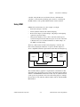
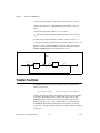
The most common tasks are interactively designing a controller, and
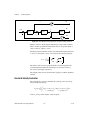
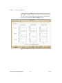
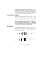
interactively studying the robustness of a given controller. Figure 2-2
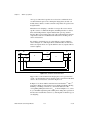
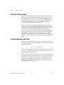
shows a simplified schematic representation of the interactive design loop.
ICDM Synthesis
Window
Designer
C(s)
ICDM Main
Window
G
Figure 2-2. Simple Representation of the Interactive Design Loop
The solid lines indicate graphical or alpha-numeric communication. The
dashed line shows the automatic export of the controller from the synthesis
window to the ICDM Main window. Notice that only one synthesis window
can be open at any given time. Also notice that for the purposes of design,
the user interacts only with the synthesis window and not with the ICDM
Main window.
© National Instruments Corporation
2-9
Xmath Interactive Control Design Module
Chapter 2
Introduction to SISO Design
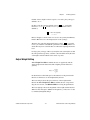
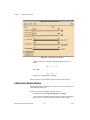
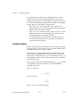
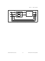
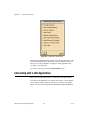
Figure 2-3 shows a simplified schematic representation of the interactive
robustness analysis loop. Here, the user interacts with the Alternate Plant
window, interactively changing the alternate plant transfer function Palt,
which is automatically exported to the ICDM Main window for analysis
and display. The user receives graphical information from the Alternate
Plant window displays and also the ICDM Main window.
Figure 2-3 shows a simplified schematic representation of the interactive
design loop.
Alternate
Plant
Window
Designer
Palt (s)
ICDM Main
Window
G
Figure 2-3. Simple Representation of the Interactive Robustness Analysis
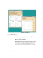
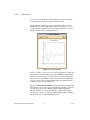
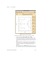
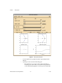
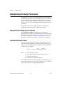
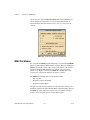
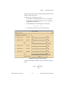
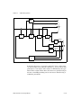
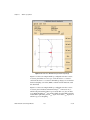
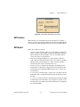
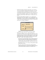
Figure 2-4 shows a simple ICDM session. The ICDM Main window is
shown at upper left, and the Pole Place Synthesis window is at lower right.
The user can drag the closed-loop poles in the Pole Place window. The
controller that is synthesized is automatically exported to the ICDM Main
window for analysis and plotting. Notice that the user’s graphical input is
mostly through the Pole Place window. The ICDM Main window is used
mostly for graphical output.
Xmath Interactive Control Design Module
2-10
ni.com
Chapter 2
Introduction to SISO Design
Figure 2-4. Simple ICDM Session
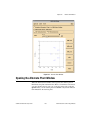
General Plotting Features
All of the plots in the ICDM Main and other windows support several
useful features: arbitrary re-ranging, zooming, data-viewing, and
interactive (graphical) re-ranging.
Ranges of Plots and Sliders
Every ICDM window has an associated Ranges window that can be used to
set the ranges of the sliders and plots appearing in the window, as well as
other parameters such as numbers of points plotted. The Ranges window
can be opened by selecting Ranges on the View or Plot menu, or by
pressing <Ctrl-R> in the window in question. In addition, every ICDM
© National Instruments Corporation
2-11
Xmath Interactive Control Design Module
Chapter 2
Introduction to SISO Design
window has an autoscale feature, which can be invoked by selecting
Autoscale on the View or Plot menu of the window. When you invoke
Autoscale, ICDM tries to assign some reasonable values to the slider and
plot scales.
Zooming
You can enlarge any portion of an ICDM plot using plot zooming. Clicking
the middle mouse button with the cursor anywhere in the plot creates a
small box containing a magnified version of the plot near the cursor. The
middle mouse button can be held down and dragged, which creates an
effect similar to dragging a magnifying glass across the plot.
Pressing <Ctrl> along with the middle mouse button (on UNIX) increases
the size of the magnified box. Clicking with the middle mouse button
increases the zoom factor. Pressing <Shift-Ctrl> along with middle mouse
button yields a large zoom box with a large magnification factor.
Zooming is a good way to read text in ICDM plots—for example, titles,
axis labels, and so on. These were intentionally made small because
zooming is easy.
Data-Viewing Plots
Pointing at or near plotted information within the ICDM windows and
clicking the right mouse button causes a small window to appear that
identifies the plot and gives the coordinates of the nearest data point
(for example, Loop Gain, L(10.1Hz) |=+11.2dB), along with its index.
This feature is called data-viewing.
If the right mouse button is clicked and dragged, the selected plot is tracked,
even if another plot comes close.
Pressing <Shift> along with the right mouse button allows the user to get
values on the piecewise linear plot that interpolates the data values. In this
case, index = 45.7 means that the selected plot point is between the 45th and
46th X-coordinate entries.
Because all ICDM plots have extensive data-viewing features, the number
of labels used to identify plots are minimal. For example, the Root Locus
plot has red and black poles and zeros shown, but no indication or label in
the plot saying what these colors mean. On a black-and-white display, you
cannot distinguish between the red and black poles/zeros. You can read in
the Help file message that the red ones correspond to the plant, and the
black ones to the controller. However, the easiest way to find out what the
Xmath Interactive Control Design Module
2-12
ni.com
Chapter 2
Introduction to SISO Design
poles and zeros are (and indeed, the only way on a black-and-white display)
is to use data-viewing.
As a general rule: To find out the meaning, purpose, or value of an object
(pole, zero, curve, and so on.) in an ICDM plot, use data-viewing.
Most objects in the ICDM Plot windows support data-viewing.
Interactive Plot Re-ranging
The range for any plot can be set in the appropriate Ranges window.
Alternatively, the ranges for plots can be interactively changed by grabbing
and dragging the axes of the plots. To make the plot range smaller, grab and
drag the appropriate axis to the desired location. A dashed line shows what
the new plot range will be. To make the plot range larger, click the left
mouse button on the appropriate axis and, while holding the button down,
move the cursor away from the plot axis. In this case you will not see a
dashed line showing the new plot range. Instead, a small box will appear
that tells you what the new range will be. The new range is given by
extrapolation of the cursor position. You can move the cursor over other
plots, and even out of the plotting window, while increasing the range of
a plot.
If a plot range is symmetric, then the new range also will be symmetric.
That is, for a symmetric plot range the minimum and maximum values for
X or Y are the same except for sign. Changing the maximum will also
change the minimum.
These changes will be exported to the Ranges window.
Graphically Manipulating Poles and Zeros
In many of the ICDM windows, the user can grab and drag poles and zeros
graphically. The paradigm of grabbing and dragging poles and zeros is
uniform across windows. Remember that you cannot always grab and drag
every pole or zero you see in an ICDM plot—for example, in the Root
Locus window, you can grab and drag any controller pole or zero, but you
cannot grab or drag a plant pole or zero.
Editing Poles and Zeros
If there is a push button labeled Edit near the plotting area, you can use it
to edit poles and zeros. If you click the Edit button, the cursor will become
a pencil symbol. Select a pole or zero by clicking the left mouse button with
the cursor positioned at the desired pole or zero. A dialog box will open that
© National Instruments Corporation
2-13
Xmath Interactive Control Design Module
Chapter 2
Introduction to SISO Design
contains variable edit boxes for the value of the pole or zero (the real and
imaginary part when the pole or zero is complex) and, if appropriate, its
multiplicity. After you enter new values, you can select OK, which will
make the changes and dismiss the dialog box, or Cancel, which will
dismiss the dialog box without making the changes.
The values you type in will not be accepted if they are invalid—for
example, a negative multiplicity for a pole or zero.
Editing Poles and Zeros Graphically
The easiest way to change a pole or zero is to grab it by clicking the left
mouse button and dragging it to the desired location. You can only drag
poles and zeros in “sensible” ways. For example, you cannot drag a single
real pole or zero off the real axis to a complex location. More precisely, the
dragging of poles and zeros works as described in the following sections.
Complex Poles and Zeros
If the pole or zero that you grab is complex, then the complex conjugate
pole or zero will automatically move as required. In this case you can drag
the pole or zero in any direction.
Isolated Real Poles and Zeros
If the pole or zero that you grab is real and not very close to another real
pole or zero, then the pole or zero motion will be constrained to the real
axis. You cannot drag the pole or zero off the real axis.
Nonisolated Real Poles and Zeros and Almost Real
Pairs
If a pair of nearby poles or zeros is very near the real axis—that is, two
nearby real poles or zeros, or a pair of complex poles and zeros with very
small imaginary part—then the dragging motion will depend on how you
originally drag the poles or zeros. If you drag it up or down, then the pair
acts as a complex pair and there is no constraint on how you can drag it. For
example, two real poles that are very close to each other can be split into a
complex pair by grabbing either one and dragging it away from the real
axis. On the other hand, if you drag the selected pole or zero left or right,
then the pair act as a real pair—the selected pole or zero then can be
dragged only along the real axis, and the other pole or zero becomes real
Xmath Interactive Control Design Module
2-14
ni.com
Chapter 2
Introduction to SISO Design
(if it was not already) but otherwise does not move. Thus, to make a pair of
complex poles real, you first drag one of them near the real axis and release.
Then you select one of these poles again, and this time drag it left or right.
This will cause the pair to become real.
Adding/Deleting Poles and Zeros
This section describes how you are allowed to add or delete poles or zeros
in some windows. Bear in mind that ICDM may not allow you to add or
delete a zero or pole in certain cases—for example, if the action would
result in a nonproper controller. In this situation, you will be warned with
a dialog box which opens.
To add a zero, click the Add Zero button that is near the plotting area, or
select the Add Zero entry from the Edit menu. In some cases there is an
accelerator for this, such as typing z in the window. These actions will
cause the cursor to become a crosshairs symbol. If you click the left mouse
button with the cursor very near the real axis, then you will create one real
zero. If you click the left mouse button with the cursor farther from the real
axis, then you will create a pair of complex conjugate zeros. Creating a pole
is similar; typing p in the window is the accelerator for creating a pole or
complex conjugate pole pair. To abort a pole or zero add operation, click
the left mouse button with the cursor outside the plot area.
To delete a pole or zero, press the <Ctrl> key near the plotting area, select
the Delete entry from the Edit menu, or enter d in the window. These
actions will cause the cursor to become a skull and crossbones symbol.
Then click the left mouse button with the cursor near the pole or zero that
you want to delete. If the pole or zero is complex, then its complex
conjugate also will be destroyed.
You always can select Undo in the Edit menu to restore deleted poles or
zeros back, provided you have not made any other changes since deleting.
To abort a delete operation, click the left mouse button with the skull and
crossbones cursor in a free area of the plot.
Adding/Deleting Pole-Zero Pairs
When you add (or delete) a pole or zero, you can drastically change the
transfer function that you are editing. In some cases, it may be better to add
(or delete) a pole-zero pair—that is, a pole and zero in exactly the same
location. Adding a pole-zero pair does not change the transfer function at
all until the pole and zero are moved apart.
© National Instruments Corporation
2-15
Xmath Interactive Control Design Module
Chapter 2
Introduction to SISO Design
To add a pole-zero pair, click the Add Pair button, select the Add Pair
entry on the Edit menu, or press <Ctrl-P> in the window. As with poles
and zeros, the pole-zero pair you create will be either real or a complex
conjugate pair, depending on how close the cursor is to the real axis
when you click the left mouse button.
After the pair is created, you can drag the pole and zero away from
each other, which results in a smooth change to the transfer function.
By convention, the cursor first grabs the zero in a pole-zero pair.
To delete a pole and zero that are very near each other, click the Delete
button, position the cursor near the pole and zero, and click the left mouse
button. This will remove the pole and zero but have little effect on the
transfer function.
If you want to delete a pole or zero that is very near a zero or pole,
respectively, then you may have to first separate them a little bit. Otherwise,
the delete command may be interpreted as a delete pair command.
Xmath Interactive Control Design Module
2-16
ni.com
3
ICDM Main Window
This chapter describes the use of the ICDM Main window, which is used to
perform the following functions:
•
Communicate with Xmath—for example, transfer plants/controllers
from/to Xmath
•
Display warning and log messages
•
Display a variety of standard plots
•
Select a synthesis method for controller design
•
Control several auxiliary windows (for example, Ranges, Alternate
Plant)
Notice that the ICDM Main window is not directly used to design the
controller. It is used to make high level decisions, such as which synthesis
method to use, and to view or analyze the response with the current
controller.
This chapter is limited to the discussion of SISO design. For MIMO design
information, refer to Chapter 11, Introduction to MIMO Design.
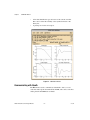
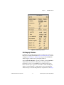
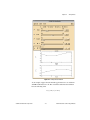
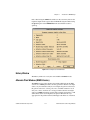
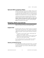
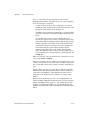
Window Anatomy
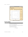
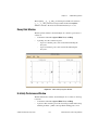
The ICDM Main window, shown in Figure 3-1, consists of the following
elements, from top to bottom:
•
A menu bar with File, Edit, Plot, Synthesis, and Help menus.
•
A scrolled text area for warnings and messages. You can resize this
area independently of the rest of the ICDM Main window. The log
messages that appear here are meant to give a rough trace of your
ICDM design session. It records major actions such as reading a
new controller or plant in, opening a new synthesis window, saving
controllers to the history list, and so on.
•
A line that gives the plant name.
© National Instruments Corporation
3-1
Xmath Interactive Control Design Module
Chapter 3
ICDM Main Window
•
A line that identifies the type and source of the current controller.
The source is either the currently active synthesis window or the
history list.
•
A plotting area for the various plots.
Figure 3-1. ICDM Main Window
Communicating with Xmath
The File menu is used to communicate with Xmath—that is, to read
controllers and/or plants from Xmath into ICDM, and to write controllers
and/or plants from ICDM back to Xmath.
Xmath Interactive Control Design Module
3-2
ni.com
Chapter 3
ICDM Main Window
Most Common Usage
In most cases, you will read a plant from Xmath at the beginning of an
ICDM design session, and write one or more controllers back to Xmath
during or at the end of an ICDM design session. This is done by selecting
the appropriate entries in the File menu.
Reading a plant into ICDM is often the first thing you do in a design
session. Before a plant is read in, the plots will be empty and you will
be unable to open any synthesis windows.
Similarly, writing the ICDM controller back to Xmath is often the last thing
you do in an ICDM design session before quitting or exiting. If the current
controller has not been written to Xmath and you attempt to exit ICDM,
a dialog box will open and ask for confirmation before exiting.
Default Plants
By selecting FileRead Default Plant, a dialog box will open which you
can use to read one of three default plants into ICDM. This default plant
dialog box is only meant to be used when you are learning how to use
ICDM and need a quick way to enter a plant. It saves you the trouble of
creating a plant in Xmath and then reading it into ICDM. It has no real use,
except in the unlikely event that your plant happens to be one of the default
plants.
Saving and Restoring an ICDM Session
The FileSave Tool button saves the entire state of the ICDM tool into an
Xmath save file. You can continue the design session at another time or on
another computer using the FileRestore Tool button.
Reading Another Plant into ICDM
When you first start ICDM, you can read a plant from Xmath using the
FileRead plant from Xmath button. After there is a plant defined in ICDM,
you can only read a new plant into ICDM from Xmath when there is no
synthesis window and the history window is not open. If you try to read a
plant when a synthesis window or the History window is open, a dialog box
will notify you that the open synthesis or History window first must be
closed.
Reading a new plant into ICDM when there already was a defined plant has
several important consequences. First, all controllers on the history list that
were designed by the Pole Place, LQG, or synthesis windows are converted
© National Instruments Corporation
3-3
Xmath Interactive Control Design Module
Chapter 3
ICDM Main Window
to a simple transfer function representation, which means that you cannot
read them back into the Pole Place, LQG, or synthesis windows because
these types depend on the plant. Also, all synthesis windows will be reset
to their initial (default) settings. Because these side effects may be
undesired, the user is warned before these actions are taken.
Reading a Controller from Xmath into ICDM
You can read a controller from Xmath into ICDM using the FileRead
Controller entry. This requires closing any open synthesis window or the
History window. Reading in a new controller will overwrite the current
controller in ICDM, so unless there is no current controller or you have
saved the current controller to the history list or Xmath, you will be warned
and asked for confirmation.
After you have read in the new controller, you can proceed with opening
a synthesis window, and the usual rules apply. If the synthesis window is
compatible with the current controller that you have just read in, the
parameters in the synthesis window will be set appropriately. If the
synthesis window is not compatible with the controller, you will be warned
that opening the synthesis window will overwrite the controller.
When you read a controller from Xmath, it is represented as a transfer
function. This means that you cannot get a controller from Xmath into
the LQG or synthesis windows.
Writing the Plant Back to Xmath
Because you cannot change the plant transfer function from inside ICDM,
the only reason to write the plant back to Xmath is if you have forgotten
what the plant transfer function is or if you fear that you may have changed
it in Xmath.
Writing the Alternate Plant back to Xmath
If you want to write the alternate plant transfer function to Xmath, use the
Special menu in the Alternate Plant window.
Writing a Controller on the History List to Xmath
If you want to write a controller that has been saved on the history list to
Xmath, you first must make it the current controller by opening the History
window and selecting it. Then use the FileWrite Controller button to write
the current controller to Xmath.
Xmath Interactive Control Design Module
3-4
ni.com
Chapter 3
ICDM Main Window
ICDM Plots
Various plots can be shown at the bottom of the main ICDM window. The
Plot menu is used to select which plots are shown, and also to magnify a
plot or set the plotting ranges. The user can choose any combination of the
following:
•
Loop transfer function magnitude
•
Loop transfer function phase
•
Sensitivity and complementary sensitivity magnitude
•
Closed-loop poles and zeros
•
Output response to a unit step input
•
Actuator response to a unit step input
•
Nyquist plot of loop transfer function
•
Nichols plot of loop transfer function
Refer to the Basic SISO Terminology section of Chapter 2, Introduction to
SISO Design, for definitions of these terms. The default plots are loop
transfer function magnitude and phase, and output and actuator response
to a unit step input.
For more information about other plots available for MIMO design, refer to
Chapter 11, Introduction to MIMO Design.
Selecting Plots
Selecting Plot»Plot Choices or pressing <Ctrl-P> in the main ICDM
window will cause a plot selection dialog box to appear, as shown in
Figure 3-2. The plot selection dialog box that appears is modal, which
means that you cannot interact with any other Xmath window until you
have dismissed this dialog by clicking Cancel or OK.
Figure 3-2. ICDM Main Window Plot Choices Dialog
© National Instruments Corporation
3-5
Xmath Interactive Control Design Module
Chapter 3
ICDM Main Window
In the ICDM Main window, the Plot Choices dialog box is used to select
any combination of the eight plots. This dialog box is modal so you cannot
interact with any other Xmath window until you dismiss it.
Ranges of Plots
The ranges for the plots can be set in the Ranges window, shown in
Figure 3-3. The Ranges window can be made to appear by selecting
Plot»Ranges or pressing <Ctrl-R> in the ICDM Main window. The
Ranges window also is used to determine the number of points used
in the plots.
ICDM provides two convenient ways to select ranges for the plots. The first
is to use the Autoscale feature which can be invoked from the Plot menu
or from the Ranges window. When Autoscale is invoked, ICDM tries to
assign sensible ranges to the plots but does not always succeed. The second
convenient method for changing the ranges of plots is to use interactive
re-ranging, which is described in the General Plotting Features section
of Chapter 2, Introduction to SISO Design.
The ICDM Ranges window, shown in Figure 3-3, is used to set the analysis
ranges and plot ranges for the ICDM Main window.
Xmath Interactive Control Design Module
3-6
ni.com
Chapter 3
ICDM Main Window
Figure 3-3. ICDM Ranges Window
Plot Magnify Windows
In addition to the standard plotting features (zooming, data-viewing, and
interactive re-ranging) described in the General Plotting Features section
of Chapter 2, Introduction to SISO Design, the plots in the ICDM Main
window support another feature: plot magnify windows.
Selecting Plot»Plot Magnify or pressing <Ctrl-M> or in the ICDM Main
window will cause the cursor to change into a crosshairs symbol.
Positioning the cursor over an ICDM plot and clicking the left mouse
button causes the plot to appear, in a new window called a Plot Magnify
window, as shown in Figure 3-4. This window can be resized using the
window manager, and can be independently re-ranged. Refer to the Ranges
© National Instruments Corporation
3-7
Xmath Interactive Control Design Module
Chapter 3
ICDM Main Window
of Plots section. If another plot is subsequently selected for magnifying,
it will replace the current plot in the plot magnify window.
The Plot Magnify window is a separate window that shows one of the
ICDM main plots. The Plot Magnify window, shown in Figure 3-4, can
be independently resized by the window manager. The ranges of the Plot
Magnify window can also be independently set.
Figure 3-4. Plot Magnify Window
It also is possible to select a portion of a plot for magnification. Click and
drag the left mouse button with the cursor in an ICDM plot. While holding
the left mouse button down, you can drag out a box (shown in dashed lines);
when you release, the dashed box becomes the range for the magnified plot.
You also can drag out a box in the magnified plot itself. This effectively
changes the range of the magnified plot.
By selecting Plot»New Plot Magnify or pressing <Ctrl-N> in the ICDM
Main window, you can select a plot for magnification. In this case, the new
plot will appear in a new Plot Magnify window. When multiple Plot
Magnify windows are open, the Plot Magnify command will send the
selected plot to the most recently created Plot Magnify window. New Plot
Magnify will create a new Plot Magnify window.
Xmath Interactive Control Design Module
3-8
ni.com
Chapter 3
ICDM Main Window
Selecting a Synthesis or History Window
The Synthesis menu in the ICDM Main window is used to select which
synthesis window will be active. If the current controller is compatible with
the requested synthesis window, then the synthesis window opens, and is
initialized with the current controller.
If the current controller is not compatible with the Synthesis menu
selected, then a dialog box appears that gives the user several options. If the
user proceeds in this case, the current controller will be replaced with the
previous design in the synthesis window selected. For example, if the Root
Locus Synthesis window is open so that the current controller is a general
transfer function, and the user requests the LQG Synthesis window, a
dialog box will issue a warning that the current design will be overwritten,
and give the user the option of cancelling the request, proceeding, or
writing the current (Root Locus) controller to the history list before
proceeding. If the user proceeds, then the Root Locus window will close,
the LQG window will open, and the current controller will be overwritten
with the controller from the LQG Synthesis window.
To open the History window, select Synthesis»History. Because all
controllers are compatible with the History window, the History window
will open with the current controller active. In other words, the current
controller will be saved on the history list (if it has not already been saved)
and made the active or selected controller on the history list.
Edit Menu
The Edit menu has two important entries:
•
Selecting EditAdd to History, or typing h in the ICDM Main window,
will cause the current controller to be saved on the history list. You will
be prompted for a comment that will be saved along with the current
controller. Refer to Chapter 9, History Window.
•
Selecting Edit»Alternate Plant window causes the Alternate Plant
window to appear. Refer to Chapter 10, Alternate Plant Window.
© National Instruments Corporation
3-9
Xmath Interactive Control Design Module
4
PID Synthesis
This chapter discusses the PID Synthesis window. This window is used to
synthesize various types of standard classical SISO controllers such as P,
PI, PD, PID, lead-lag, and lag-lead. However, the controller that is
designed by the PID Synthesis window will be referred to as a PID
controller even if it has some other form such as PI. Multivariable (MIMO)
PID controllers can be synthesized using the Multiloop Synthesis window.
Refer to Chapter 13, Multi-Loop Synthesis.
Window Anatomy
The PID Synthesis window is shown in Figure 4-1. It consists of the
following, from top to bottom:
•
A menu bar with entries Special, Edit, View, and Help.
•
A text area that displays the transfer function of the current PID
controller.
•
A control panel with five rows, each of which corresponds to one
design parameter. A Bode plot of the controller transfer function with
handles for graphically manipulating the design.
PID Controller Terms
The overall controller transfer function is given by the product of up to five
terms, each of which depends on one parameter. The five parameters and
corresponding terms in the controller are shown in Table 4-1, from top to
bottom.
Table 4-1. PID Controller Terms and Parameters
Term
Parameter
Symbol
Controller
Proportional (P)
Gain
Kp
Kp
Integral (I)
Integral time constant
Tint
1 + 1/(sTint)
Derivative (D)
Derivative time constant
Tdiff
1 + sTdiff
© National Instruments Corporation
4-1
Xmath Interactive Control Design Module
Chapter 4
PID Synthesis
Table 4-1. PID Controller Terms and Parameters (Continued)
Term
Parameter
Symbol
Controller
HF rolloff 1
HF rolloff time 1
Thf 1
1 + 1/(sThf 1)
HF rolloff 2
HF rolloff time 2
Thf 2
1 + 1/(sThf 2)
Toggling Controller Terms On and Off
For each parameter, the toggle button at the left of the row is used to toggle
the terms on and off. “On” means that the corresponding controller term
appears in the overall controller transfer function, and the slider and
variable edit box can be used to change the parameter. “Off” means that the
controller term does not appear in the overall controller transfer function.
In this case, the slider and the variable-edit box are read-only—you cannot
drag the slider, and you cannot type in the variable-edit box. When the
button is turned on again, the parameter value is restored to its previous
value. You can use the buttons to do a quick A/B comparison of a PID
controller with or without a given term—for example, to see the effect of
a high frequency rolloff term or integral action.
Xmath Interactive Control Design Module
4-2
ni.com
Chapter 4
PID Synthesis
Figure 4-1. PID Synthesis Window
As an example, suppose that the P and I toggle buttons are on, and the D
and HF rolloff buttons are off. The controller transfer function will then
have the following form:
C ( s ) = K p + ( 1 ⁄ sT int )
© National Instruments Corporation
4-3
Xmath Interactive Control Design Module
Chapter 4
PID Synthesis
Notice that there are at least two other commonly used forms for a PID
control law that differ from the one used in ICDM:
C ( s ) = K p + ( 1 + 1 ⁄ T int s + T diff s )
and
C ( s ) = K p + 1 ⁄ T int s + T diff s
ICDM enforces a proper controller transfer function, that is, a finite high
frequency gain. Therefore, if the D term is on, ICDM will require at least
one HF rolloff term also to be on.
Opening the PID Synthesis Window
When you select the PID window from the Synthesis menu in the ICDM
Main window, the PID window first decides whether the current controller
transfer function has the form of a PID controller. If it does, then the PID
window sets its parameters (including the push buttons) to the values that
would yield the current controller, and then opens. In this case the current
controller remains unchanged. If the current controller does not have the
form of a PID controller, then a dialog box appears and warns the user and
offers several alternatives.
Manipulating the Controller Parameters
Each parameter can be changed using the slider, variable-edit box, or
graphically. To change the sign of the parameter or to change the parameter
to a value outside the current slider or plot range, you must use the
variable-edit box. Notice that negative values are allowed, but often
are not what you want.
The parameters also can be changed graphically by grabbing and dragging
the controller Bode plot in the following ways:
•
To change the gain, with the gain parameter turned on, grab the
magnitude Bode plot anywhere except near the handles (dark circles)
on the plot. You now can drag the Bode plot up and down, which
changes the gain.
•
To change the other parameters, listed in column four of Table 4-1,
grab the appropriate handle (dark circle) on either plot and drag it left
and right to the desired frequency, which is the inverse of the time
parameter. The associated slider and variable-edit box also will be
updated as you drag the handle.
Xmath Interactive Control Design Module
4-4
ni.com
Chapter 4
PID Synthesis
Time Versus Frequency Parameters
Notice that the sliders and variable-edit boxes use time parameters,
whereas the Bode plot handles use frequencies, that is, the inverses of the
time parameters. If you think of integral action as being parameterized by
a characteristic time, then you may prefer to use the slider. If you think of
integral action as being parameterized by a characteristic frequency (reset
rate), then you may prefer to manipulate the Bode plot handle.
Ranges of Sliders and Plots
The ranges for the sliders and plots can be changed in several ways. If you
enter a value that lies outside the slider range in the corresponding variable
edit box, the range of the slider will automatically adjust to accommodate
the new value. You also can change the range of a slider using the Ranges
window, which appears when you select View»Ranges or press <Ctrl-R>
in the PID window. Selecting View»Auto Scale will cause ICDM to select
sensible values for the slider and plot ranges based on the current controller.
The ranges for the plots also can be changed interactively. Refer to the
General Plotting Features section of Chapter 2, Introduction to SISO
Design.
Controller Term Normalizations
Each of the controller terms is normalized in a way that is convenient for
most PID design tasks as described in the following sections.
Integral Term Normalization
The integral term is high-frequency normalized, which means that it is
approximately one for frequencies above 1/Tint. Therefore, you can adjust
the integral time constant 1/Tint without significantly affecting the
controller transfer function at high frequencies. For example, you can add
integral action to a controller without significantly affecting the stability
margins or closed-loop dynamics by adding the integral term with 1/Tint
well below the crossover frequency, that is, 1/Tint large. In this case, your
controller will enforce steady-state tracking, but over a time period longer
than the closed-loop system dynamics. You then can slowly decrease 1/Tint
until you get a good balance between fast integral action and the
degradation of stability margins.
© National Instruments Corporation
4-5
Xmath Interactive Control Design Module
Chapter 4
PID Synthesis
Derivative Term Normalization
The derivative term is low-frequency normalized, which means that at low
frequencies (below 1/Tdiff) it is nearly one, and so has little effect on the
overall controller transfer function at low frequencies. In particular, the
loop transfer function at s = 0 is not affected by the derivative term at all,
so static tracking, static actuator effort, and so on are not affected by the
derivative term. You can start by making the Tdiff term small and then
gradually increasing it until you get a good balance between better stability
margins and excessive actuator effort.
Rolloff Term Normalization
The two HF rolloff terms are low-frequency normalized, so they have little
effect at frequencies below Thf. You can start with small values for these
parameters, and then gradually increase them until you start to notice a
degradation in stability.
Xmath Interactive Control Design Module
4-6
ni.com
5
Root Locus Synthesis
This chapter describes the user interface, terminology, and parameters used
for root locus synthesis.
Overview
The Root Locus window performs two main functions:
•
Displays selected gain and phase contours in the complex plane of the
loop transfer function.
•
Allows the user to manipulate the controller transfer function
graphically by dragging controller poles and zeros, or dragging
the closed-loop poles along the root locus plot.
The Root Locus window only works in SISO mode.
Window Anatomy
The Root Locus Synthesis window is shown with the standard (default)
contour in Figure 5-1. The branches of the locus connect the zeros and
poles of the loop transfer function, which are shown in the plot. The
closed-loop poles, which are on the locus, also are shown.
© National Instruments Corporation
5-1
Xmath Interactive Control Design Module
Chapter 5
Root Locus Synthesis
Figure 5-1. Root Locus Synthesis Window
The Root Locus Synthesis window consists of, from top to bottom:
•
A menu bar with entries Special, Edit, View, and Help.
•
A slider and variable edit box for the gain. These controls are used
to show and also to change the controller gain. The gain also can be
changed graphically by dragging the closed-loop poles along the root
locus.
•
(Bottom left) The root locus plot. The plot shows selected phase or
gain contours of the loop transfer function along with the plant and
controller poles and zeros. A more detailed description appears
following.
•
(Bottom right) Buttons to add/delete/edit poles and/or zeros. Poles,
zeros, and pole-zero pairs also can be created and destroyed using the
Xmath Interactive Control Design Module
5-2
ni.com
Chapter 5
Root Locus Synthesis
Edit menu or by typing the accelerators in the Root Locus window.
A more detailed description appears following.
The Root Locus Synthesis window is shown in Figure 5-1 with the standard
(default) 180° contour. The branches of the locus connect the zeros and
poles of the loop transfer function, which are shown in the plot. The
closed-loop poles, which are on the locus, are also shown.
Opening the Root Locus Synthesis Window
The Root Locus window can accept any type of controller, so it can always
be opened. It simply reads the current controller from ICDM. You then can
use the Root Locus window to manipulate the controller poles, zeros, and
gain.
After you have changed the controller using the Root Locus window, the
controller loses any special form it may have had—for example, LQG.
It is represented by its transfer function. Thus, you can use the Root Locus
window to change the zeros, poles, and gain of a controller originally
designed using the LQG window, but you then cannot read the controller
back into the LQG Synthesis window since it is no longer an LQG
controller.
Terminology
The loop transfer function is expressed in the following product form:
( s – z 1 )… ( s – z k )
L ( s ) = K ---------------------------------------------( s – p 1 )… ( s – p 1l )
where K is called the gain (notice that the gain is high-frequency
normalized), the zi values are the zeros of the loop transfer function
and the pi values are the poles of the loop transfer function.
Each of these poles and zeros is associated with either the plant or the
controller. The Root Locus window allows you to change the gain, change
or delete any controller pole or zero, or create new controller poles and
zeros as long as the controller transfer function remains proper—that is, has
finite gain at high frequencies. The Root Locus window will not allow you
to change or delete any plant pole or zero. The Alternate Plant window can
be used to modify the plant interactively and see the effect on the
closed-loop system performance.
© National Instruments Corporation
5-3
Xmath Interactive Control Design Module
Chapter 5
Root Locus Synthesis
Plotting Styles
Selecting View»Locus Select or pressing <Ctrl-L> in the Root Locus
window produces a dialog box in which the user can choose one of many
possible plotting styles. In all cases, the (open-loop) controller and plant
poles and zeros are shown on the plot. On color displays:
•
Controller poles and zeros are black
•
Plant poles and zeros are red
This serves as a mnemonic: you can manipulate black but not red poles or
zeros. On monochrome displays, the plant poles and zeros are lighter than
the controller poles and zeros. You can always use data-viewing to obtain
more information about a pole or zero. Refer to the Data-Viewing Plots
section of Chapter 2, Introduction to SISO Design. Figure 5-2 shows a
dialog box for choosing plotting style with standard (default) contours
selected.
Figure 5-2. Root Locus Select Dialog for Choosing Plotting Style
Xmath Interactive Control Design Module
5-4
ni.com
Chapter 5
Root Locus Synthesis
Phase Contours
For each of magnitude and phase contours, you can choose one of three
possible plotting styles.
•
180°
The plot shows the locus of points where the phase angle of the loop
transfer function is 180°. This yields a conventional root locus display.
This is the default phase contour plotting style. The plot shows the set
of all possible closed-loop pole locations as the gain is swept from
0 to ∞.
•
160°
200°
10°
The plot shows the loci of points where the phase angle of the loop
transfer function is 160°, 170°, 180°, 190°, or 200°. These plots show
the set of all possible closed-loop pole locations as the gain is swept
from 0 to and there is an additional phase shift of ±20°, ±10° in the
loop transfer function.
•
None
No phase contours are plotted.
Magnitude Contours
•
0 dB
The plot shows the locus of points where the magnitude of the loop
transfer function (including the delay, if applicable) is 0 dB.
•
–2:2 dB
The plot shows the loci of points where the magnitude of the loop
transfer function is –2, –1, 0, +1, and +2 dB, respectively.
•
None
No magnitude contours are plotted. This is the default magnitude
contour plotting style.
Notice that by selecting None for both phase and magnitude contours, the
plot shows only the controller and plant poles and zeros. This is useful for
graphically editing the controller poles and zeros.
If any phase contours are plotted, the closed-loop poles are shown (in blue
on a color display). They can be dragged along the 180° contour plot.
© National Instruments Corporation
5-5
Xmath Interactive Control Design Module
Chapter 5
Root Locus Synthesis
All of the plots support data viewing: click the right mouse button with the
cursor positioned near a pole, zero, or one of the plots. This allows you to
find the gain associated with a particular point on a phase contour, for
example.
Slider and Plot Ranges
To change the ranges of the Gain slider or the root locus plot, select
View»Ranges or press <Ctrl-R> in the Root Locus window.
The slider range also will be changed automatically if you type a new value
which is outside the current range in the corresponding variable edit box.
The plot also can be re-ranged interactively by grabbing and dragging the
plot axes. Refer to the discussion of plot re-ranging in section
s-plots-features.
Selecting View»Auto-scale or pressing <Ctrl-A> in the Root Locus
window will cause new ranges to be assigned to the slider and plot, based
on the current controller.
Manipulating the Parameters
The Graphically Manipulating Poles and Zeros section of Chapter 2,
Introduction to SISO Design, describes how to graphically manipulate the
controller poles and zeros.
The Root Locus window enforces a proper controller; that is, the controller
must have at least as many poles as zeros. If you attempt to add one zero or
a pair of zeros, that would result in more controller zeros than poles, a
warning is issued. Similarly, you cannot delete one or more controller
poles, if the deletion would result in an improper controller.
You can select Edit»Undo to restore the deleted pole(s) and/or zero(s),
provided you have not made any other changes since deleting. To abort a
delete operation, click the left mouse button with the skull and crossbones
cursor away from any pole or zero.
Xmath Interactive Control Design Module
5-6
ni.com
Chapter 5
Root Locus Synthesis
Design
This section gives short descriptions of how the Root Locus window can be
used to design or analyze controllers. This section also provides some
interpretations and describes some uses of the nonstandard contour plots.
Adding a Pole-Zero Pair
Adding a pole-zero pair is a good way to add a little lead or lag action to an
existing controller. When you first add the pole-zero pair, you will not have
changed the controller transfer function. As you grab the zero and drag it
away from the pole, you will induce a smooth change in the controller
transfer function. By dragging the zero a little closer to the origin, you will
add a small amount of lead action to the controller—that is, increase the
controller phase for frequencies between the pole and zero, and increase the
magnitude at frequencies larger than the pole.
Similarly, by dragging the zero away from the origin, you will create some
lag action—that is, decrease the loop phase between the zero and pole, and
increase the gain below the pole frequency.
Deleting Pole-Zero Pairs
Deleting a controller pole-zero pair is a good way to do interactive
controller model reduction. Suppose that you have synthesized a suitable
controller and need to find a lower order controller that has nearly the same
performance. Using the Root Locus window, you want to move (stable)
controller poles or zeros near each other without sacrificing controller
performance. Good candidates are poles and zeros substantially outside the
control system bandwidth, or pairs of nearby poles and zeros. After you
have moved a controller pole or zero (or both) so that they are near each
other—and hopefully, control system performance has not changed too
much—then you can delete the pair without severely affecting the
controller transfer function. You have just reduced the controller order by
one (or two, if you deleted a complex conjugate pair of poles and zeros).
© National Instruments Corporation
5-7
Xmath Interactive Control Design Module
Chapter 5
Root Locus Synthesis
Interpreting the Nonstandard Contour Plots
The Root Locus window can display phase contours other than the standard
180° as well as various magnitude contour plots. The meaning of these
curves is simple: if L(s) = a, then s would be a closed-loop pole if the loop
transfer function were multiplied by –1/a at the frequency s. For example,
a point s labeled ⏐L(s)⏐ = –3 dB on one of the 170° curves would be a
closed-loop pole if the loop transfer function at the frequency were to
increase in magnitude by 3 dB and increase in phase by 10°.
This simple observation works two ways. Continuing the previous
example, to have a pole at s, try to change the current controller to achieve
the required phase shift +10° and gain increase (+3 dB) at (for example,
by adding an appropriate pole-zero pair).
On the other hand, if the complex number is a poor place for a closed-loop
pole (for example, very lightly damped or unstable), then the current
compensator is not robust, since only a 10° phase shift along with 3 dB
of gain change in loop gain (most likely, the plant) would result in a
closed-loop pole at s. In this case, you turn to the problem of synthesizing
new compensation which decreases the phase and magnitude of the loop
transfer function at the frequency s. This has the effect of making the
closed-loop system less likely to have a pole at s when the plant transfer
function is changed; that is, it results in a more robust design.
Figure 5-3 shows the Root Locus window with the phase contours turned
off and the 0 dB magnitude contour turned on. The locus shows the set
of all possible closed-loop poles for the modified loop transfer function
L(s) = e jθL(s) as θ varies from zero to 2π. By data-viewing the contour,
you can find the phase shift (value of θ) that corresponds to any point on
the locus.
Xmath Interactive Control Design Module
5-8
ni.com
Chapter 5
Root Locus Synthesis
Figure 5-3. Root Locus Synthesis Window with the 0 dB Magnitude Contour
© National Instruments Corporation
5-9
Xmath Interactive Control Design Module
6
Pole Place Synthesis
This chapter discusses the Pole Place Synthesis window, which is used to
design a SISO controller by assigning the closed-loop poles. Pole Place
operates in two modes:
•
Normal mode (integral action not enforced)
•
Integral action mode
The Pole Place Synthesis window cannot be used to design MIMO
controllers.
Window Anatomy
The Pole Place window is shown in Figure 6-1. From top to bottom,
it consists of:
•
A menu bar with entries Special, Edit, View, and Help.
•
A toggle button used to set normal or integral action mode.
•
A slider and variable-edit box used to time or frequency-scale the
closed-loop poles.
•
A plot used to display and manipulate the closed-loop poles.
•
Buttons used to manipulate the closed-loop poles.
© National Instruments Corporation
6-1
Xmath Interactive Control Design Module
Chapter 6
Pole Place Synthesis
Figure 6-1. Pole Place Synthesis Window
Pole Place Modes
In Pole Place, the user selects either closed-loop poles (in normal mode) or
2n + 1 closed-loop poles (in integral action mode). These poles uniquely
determine the controller transfer function.
This process can be described in terms of the coefficients of the plant and
controller numerators and denominators.
The plant transfer function is given by
P(s) = np(s)/dp(s)
Xmath Interactive Control Design Module
6-2
ni.com
Chapter 6
Pole Place Synthesis
where
dp(s) = sn + a1sn–1 + a2sn–2 + ... + an
np(s) = b0sn + b1sn–1 + ... + abn
Notice that the order of the plant is n, and allow the possibility that the plant
transfer function is not strictly proper; that is, the plant can have as many
zeros as poles.
Normal Mode
In normal mode, the order (number of poles) of the controller is fixed and
equal to n (the order of the plant), so there are a total of 2n closed-loop
poles. In this case, the 2n degrees of freedom in the closed-loop poles
exactly determine the controller transfer function, which also has 2n
degrees of freedom.
In normal mode, the controller transfer function has order n and is strictly
proper:
C(s) = nc(s)/dc(s)
where
dc(s) = sn + x1sn–1 + x2sn–2 + ... + xn
nc(s) = y1sn–1 + y2sn–2 + ... + 2yn
Therefore, the closed-loop characteristic polynomial has degree 2n:
χ ( s ) = n c ( s )n p ( s ) + d c ( s )d p ( s )
= ( s – λ 1 ) ( s – λ 2 )… ( s – λ 2n )
= (s
2n
+ α1 s
2n – 1
+ … + α2 n )
where λ1, …, λ2n are the closed-loop poles chosen by the user.
© National Instruments Corporation
6-3
Xmath Interactive Control Design Module
Chapter 6
Pole Place Synthesis
We can write this polynomial equation as follows:
b0
0
…
0
b1
b0
…
0
b2
b1
…
0
…
bn – 1 bn – 2
…
b0
bn bn – 1
b1
0
bn
b2
0
0
b3
0
…
bn
…
0
…
x1
·
1
a1
0
1
…
…
0
0
a2
a1
…
0
…
an – 1 an – 2
…
1
·
an an – 1
a1
xn
0
an
a2
0
0
a3
0
…
an
·
+
…
0
…
y1
·
· +
·
yn
a1
…
α1
a
n
+
= …
0
α 2n
…
0
These 2n linear equations are solved to find the 2n controller parameters
x1, ..., xn and y1, ..., yn.
Integral Action Mode
The degree (number of poles) of the controller is fixed and equal to n + 1,
so there are a total of 2n + 1 closed-loop poles. In this case, the 2n + 1
degrees of freedom in the closed-loop poles, along with the constraint that
the controller must have at least one pole at s = 0, exactly determine the
controller transfer function. In fact, the closed-loop poles give a complete
parameterization of all controllers with at least one pole at s = 0, and n or
fewer other poles.
Equations similar to those shown in the Normal Mode section are used to
determine the controller parameters given the closed-loop pole locations.
Xmath Interactive Control Design Module
6-4
ni.com
Chapter 6
Pole Place Synthesis
State-Space Interpretation
In a state-space framework, it is common to classify the closed-loop poles
as n “control eigenvalues” and n “estimator eigenvalues.” But, in fact, it
makes no difference in the final controller transfer function how you
classify the closed-loop poles.
In other words, in a state-space framework, swapping a “control
eigenvalue” and an “estimator eigenvalue” will result in different feedback
and estimator gains, but the same final controller.
Opening the Pole Place Window
The Pole Place window can accept any controller with n poles, or n + 1
poles provided the controller has at least one pole at s = 0. The Integral
Action toggle button will be properly set. In particular, it accepts all LQG
and H∞ controllers. This allows the user to manually tune the closed-loop
poles in a design that was, originally, LQG or H∞. In this case, you cannot
read the resulting controller back into the LQG or window since the
controller no longer has this special form.
Manipulating the Closed-Loop Poles
The closed-loop poles and zeros can be dragged and edited interactively.
Refer to the Graphically Manipulating Poles and Zeros section of
Chapter 2, Introduction to SISO Design, for a general discussion of
manipulating poles graphically.
Time and Frequency Scaling
The slider and variable-edit box show the average value of the closed-loop
pole magnitudes, and therefore can be interpreted as, roughly, the
bandwidth of the closed-loop system. The average frequency is given by:
Favg = ⏐λ1λ2 ... λ2n⏐1/2n
where λ1, ..., λ2n are the closed-loop poles. Notice that the average is
geometric.
You can change Favg by dragging the slider or typing into the variable edit
box. The effect is that the closed-loop poles are all multiplied by a scale
factor in such a way that becomes the requested value. Therefore, by
changing Favg, you are time- or frequency-scaling the closed-loop
dynamics.
© National Instruments Corporation
6-5
Xmath Interactive Control Design Module
Chapter 6
Pole Place Synthesis
A circle of radius Favg also is displayed in the plot. You also can drag the
circle to change Favg.
Butterworth Configuration
Click the Butterworth button to move the poles to a Butterworth
configuration, preserving Favg. The initial pole configuration also is
set to Butterworth.
Editing the Closed-Loop Poles
You can change the closed-loop poles two ways: by editing or by grabbing
and dragging them. Both of these methods are described in the General
Plotting Features section of Chapter 2, Introduction to SISO Design.
Slider and Plot Ranges
To change the ranges of the Frequency Scaling slider or the plot of
closed-loop poles, select View»Ranges or press <Ctrl-R> in the Pole Place
window.
The slider range also will be changed automatically if you type a new value
which is outside the current range in the variable edit box. The plot also can
be re-ranged interactively by grabbing and dragging the plot axes; refer to
the General Plotting Features section of Chapter 2, Introduction to SISO
Design.
Selecting View»Auto-scale or pressing <Ctrl-A> in the Root Locus
window will cause new ranges to be assigned to the slider and plot,
based on the current controller.
Xmath Interactive Control Design Module
6-6
ni.com
7
LQG Synthesis
This chapter discusses the LQG Synthesis window, which is used to
synthesize a linear quadratic Gaussian (LQG) controller for a SISO plant.
If you select LQG synthesis with a MIMO plant, you will get the MIMO
LQG Synthesis window described in Chapter 12, LQG/H-Infinity
Synthesis.
LQG Synthesis Window Anatomy
The LQG Synthesis window is shown in Figure 7-1. From top to bottom,
it contains:
•
A menu bar with entries Special, Edit, View, and Help.
•
A message area that describes the synthesis mode (type of controller);
for example, LQG with integral action.
•
A control panel for changing the four design parameters:
–
Control cost parameter (ρ)
–
Sensor noise parameter (υ)
–
Integral action time constant (Tint)
–
Decay rate or exponential time weighting parameter (a)
These parameters are described in greater detail later in this chapter.
© National Instruments Corporation
7-1
Xmath Interactive Control Design Module
Chapter 7
LQG Synthesis
Figure 7-1. LQG Synthesis Window
•
A control panel used to graphically edit the output weight transfer
function.
•
A plotting area that contains the following plots:
–
Xmath Interactive Control Design Module
The symmetric root locus plots of the control and estimator
closed-loop poles. The control cost and sensor noise parameters
can be changed by dragging the closed-loop poles along the plot.
7-2
ni.com
Chapter 7
LQG Synthesis
If the decay rate is enabled, it is shown as a vertical line that can
be dragged.
–
A plot showing the poles and zeros of the output weight transfer
function. If weight zero editing is enabled, the zeros can be edited
graphically.
–
A plot showing the magnitude of the output weight transfer
function.
Synthesis Modes
In addition to standard LQG synthesis, the LQG Synthesis window
supports any combination of three optional features:
•
Integral action
•
Exponential time weighting (guaranteed decay rate)
•
Output weight editing
The synthesis mode is reported in the text at the top of the window. The
toggle Int Time (integral action time) button enables and disables integral
action. The Decay Rate toggle button controls exponential time weighting.
The Weight Zero Edit toggle button enables and disables output weight
editing.
Opening the LQG Synthesis Window
The LQG window can only accept LQG controllers. If the current
controller is of type LQG (perhaps, from the History window) and the LQG
window is opened, the current controller is read into the LQG window.
That is, the push buttons and parameters are set to the appropriate values.
If the current controller is not of type LQG, and the user attempts to open
the LQG Synthesis window, a dialog box appears and warns the user that
proceeding with opening the LQG Synthesis window will overwrite the
current controller with the LQG controller.
The LQG window remembers its parameter settings. When it is opened, the
parameters will be exactly as they were when the LQG window was last
closed, or it will be set to default values if the LQG window has not been
opened in this ICDM session.
© National Instruments Corporation
7-3
Xmath Interactive Control Design Module
Chapter 7
LQG Synthesis
Setup and Terminology
The different modes are described using the following basic terminology:
y = P ( u + w proc )
u = ( – C ) ( y + w sens )
y˜ = Wy
Figure 7-1 shows a block diagram with the basic setup for LQG synthesis,
where
u is the actuator signal (output of the controller)
wproc is an (input referred) process noise
y is the (plant) output signal
y˜ is the weighted output signal
wsens is a sensor noise
P is the plant transfer function
C is the controller transfer function
W is the output weight transfer function
The noises wproc and wsens are white; that is, they have constant power
spectral densities (PSDs). The parameter υ is the ratio of the PSD of wsens
to the PSD of wproc.
r=0
y
u
C(s)
y
W(s)
P(s)
wproc
wsens
Figure 7-2. Block Diagram Showing the Basic Setup for LQG Synthesis
Standard LQG (All Toggle Buttons Off)
In LQG synthesis mode, the controller minimizes a weighted sum of the
steady-state actuator and output variance:
2
2
J = lim E ( ρu ( t ) + y ( t ) )
t→∞
where E denotes expectation, ρ is the Control cost parameter, and the
parameter ν gives the ratio of the intensity of the sensor noise wsens to the
intensity of the process wproc noise (which are assumed to be white).
Xmath Interactive Control Design Module
7-4
ni.com
Chapter 7
LQG Synthesis
Integral Action
When integral action is enabled, the controller minimizes a variation on the
LQG cost:
2
2
2
J = lim E ( ρu ( t ) + y ( t ) + z ( t ) )
t→∞
where
t
∫
z ( t ) = ( 1 ⁄ T int ) y ( τ ) dτ
0
As in the standard mode, the sensor noise parameter ν is the ratio of the
sensor noise intensity to the input-referred process noise intensity.
Penalizing the “running integral” of the plant output forces the power
spectral density of the plant output to vanish at zero frequency.
In classical control terms, this forces a pole at S = 0 in the loop transfer
function, that is, integral control. As with PID design, the parameter Tint
gives the time scale over which the effects of the integral action will take
place.
Exponential Time Weighting
When this feature is enabled, the plant is first changed to P(s – a), where a
is the Decay Rate parameter. In other words, the plant is made less stable;
its poles (and zeros) are shifted to the right by the value a. Then, the LQG
controller for this “destabilized” plant is computed. Finally, the poles and
zeros of this controller are shifted left by the Decay Rate parameter a.
One effect of this shifting is that the closed-loop poles are guaranteed to
have real part less than the Decay Rate parameter a. In other words, the
closed-loop time domain responses are guaranteed to decay at least as fast
as exp(–at). This is why the parameter is called Decay Rate.
© National Instruments Corporation
7-5
Xmath Interactive Control Design Module
Chapter 7
LQG Synthesis
Output Weight Editing
When Weight Zero Edit is enabled, the LQG controller is based on
y˜ = Wy, which is a filtered version of the plant output signal y. Without
integral action, the controller minimizes the quantity:
2
2
J = lim E ( ρu ( t ) + y ( t ) )
t→∞
and with integral action, the quantity:
2
2
2
J = lim E ( ρu ( t ) + y ( t ) + z ( t ) )
t→∞
where
t
∫
z ( t ) = ( 1 ⁄ T int ) y˜ ( τ ) dτ
0
The transfer function W is the output weighting transfer function. When
W = 1, this reduces to the standard LQG controller described previously.
The weighting transfer function is given by:
W ( s ) = nw ( s ) ⁄ np ( s )
Its denominator is fixed and equal to the numerator of the plant transfer
function. Its numerator can be manipulated by the user.
The lower left plot shows the poles and zeros of the weight transfer function
W. When Weight Zero Edit is enabled, the user can grab and drag the zeros
shown, or Add/Delete/Edit zeros using the push buttons.
The lower right plot shows the magnitude of the weight transfer function.
When it is flat and equal to 0 dB for all frequencies, you have W = 1, that
is, standard LQG design based on the plant output y. When, for example, W
is larger than 0 dB at low frequencies, this means that the LQG controller
is based on a filtered version of y that emphasizes low frequencies, which
presumably results in a controller with larger loop gain at low frequencies.
Xmath Interactive Control Design Module
7-6
ni.com
Chapter 7
LQG Synthesis
State-Space Interpretation
In LQG theory, the closed-loop poles consist of n “optimal control
eigenvalues” and n “estimator (Kalman filter) eigenvalues.” For
multivariable systems, the optimal control and the optimal estimator
play different roles in the control system. But in the single-actuator,
single-sensor case, the roles are completely symmetric.
In particular, swapping the parameters ρ and ν yields the same final LQG
controller. This symmetry is broken if you use either output weighting or
integral action, however.
Manipulating the Design Parameters
The design parameters ρ and ν can be changed using the associated sliders
or the variable edit boxes. If you type in a value that is outside the current
slider range, the slider range will automatically adjust. You can change the
ranges for the sliders using the Ranges window.
The parameters Tint and a can be manipulated using the sliders or variable
edit boxes provided the associated toggle button is on. If the toggle button
is off, then the slider and variable edit box are insensitive; you cannot drag
the slider handle, and you cannot type into the variable edit box.
When the toggle buttons are turned on again, the parameters are restored to
their previous (or default) values.
Manipulating the Design Parameters Graphically
The design parameters also can be manipulated graphically as follows:
•
The closed-loop poles are shown on the two symmetric root locus
plots. They can be dragged along the root locus plot, which results
in setting the parameters ρ or ν appropriately.
•
When the Decay Rate toggle button is on, a dashed line appears in the
symmetric root locus plots, showing ℜs = a. You can drag this line left
and right to set the Decay Rate parameter.
•
When Weight Zero Editing is enabled, the user can graphically
manipulate the zeros of the weight transfer function W on the plot
labeled Weight Poles & Zeros. Refer to the Graphically
Manipulating Poles and Zeros section of Chapter 2, Introduction to
SISO Design, for a general discussion of how to move, add, delete,
or edit these zeros graphically.
© National Instruments Corporation
7-7
Xmath Interactive Control Design Module
Chapter 7
LQG Synthesis
Ranges
To change the ranges of the sliders or plots, select View»Ranges or enter
R in the LQG window.
The slider ranges also will be changed automatically if you type a new
value which is outside the current range into the corresponding variable edit
box. The plot also can be re-ranged interactively by grabbing and dragging
the plot axes; refer to the Interactive Plot Re-ranging section of Chapter 2,
Introduction to SISO Design.
Selecting View»Auto-scale or pressing <Ctrl-A> in the LQG window
causes new ranges to be assigned to the sliders and plots, based on the
current controller.
Xmath Interactive Control Design Module
7-8
ni.com
8
H-Infinity Synthesis
This chapter describes the H∞ Synthesis window used for SISO plants.
The H∞ Synthesis window is used to synthesize a central controller. Such
controllers are sometimes called linear exponential quadratic Gaussian
(LEQG) or minimum entropy controllers. For a description of the MIMO
Synthesis window, refer to Chapter 12, LQG/H-Infinity Synthesis.
H-Infinity Synthesis Window Anatomy
The H∞ Synthesis window is shown in Figure 8-1. From top to bottom,
it consists of:
•
A menu bar with entries Special, Edit, View, and Help.
•
A control panel for changing the three design parameters:
–
H∞ performance level (γ)
–
Control cost parameter (ρ)
–
Sensor noise parameter (ν)
These parameters are described in greater detail later in this chapter.
•
A control panel used to edit the output weight transfer function
(described in the Output Weight Editing section).
•
A plotting area that contains four plots:
© National Instruments Corporation
–
A singular value plot of the normalized closed-loop transfer
matrix along with the parameter γ, which can be grabbed and
dragged to a new value. If a lower bound on the minimal value
of γ is known, it also is displayed.
–
A plot that shows the closed-loop poles.
–
A plot that shows the poles and zeros of the output weight transfer
function. When Weight Zero Edit is enabled, the user can grab
and drag the zeros to new locations.
–
A plot that shows the magnitude of the output weight transfer
function.
8-1
Xmath Interactive Control Design Module
Chapter 8
H-Infinity Synthesis
Figure 8-1. H-Infinity Synthesis Window
Xmath Interactive Control Design Module
8-2
ni.com
Chapter 8
H-Infinity Synthesis
Opening the Synthesis Window
The H∞ window can only accept H∞ controllers. If the current controller is
of type H∞ (perhaps from the History window) and the H∞ window is
opened, the current controller is read into the H∞ window; that is, the
parameters are set to the appropriate values.
If the current controller is not of type H∞, and the user attempts to open
the H∞ Synthesis window, a dialog box appears and warns the user that
proceeding with opening the synthesis window will overwrite the current
controller with the controller.
The H∞ window remembers its parameter settings. When it is opened, the
parameters will be exactly as they were when the window was last closed,
or they will be set to default values if the H∞ window has not been opened
in this ICDM session.
Setup and Synthesis Method
This section describes the closed-loop transfer matrix (refer to Figure 8-2).
The H∞ synthesis procedure can be described using the following standard
setup:
y = P ( u + w1 )
z1 =
where
ρu
u = ( – C ) ( y + νw 2 )
z2 = Wy
y is the plant output signal
w1 is a normalized (input-referred process) noise
w2 is a normalized (sensor) noise
z1 is the normalized actuator signal
z2 is the weighted plant output signal
P is the plant transfer function
C is the controller transfer function
W is the output weight transfer function
© National Instruments Corporation
8-3
Xmath Interactive Control Design Module
Chapter 8
H-Infinity Synthesis
z1
u
r=0
z2
y
C(s)
W(s)
P(s)
w1
w2
Figure 8-2. Block Diagram Showing the Basic Setup for H-Infinity Synthesis
Figure 8-2 shows a block diagram with the basic setup for H∞ synthesis
where closed-loop transfer matrix H relates the two exogenous inputs w1
and w2 to the two outputs z1 and z2.
The design is based on H, the closed-loop transfer matrix relating the noises
w1 and w2 to the signals z1 and z2. H is given by the following equation:
1
H = ----------------- – ρPC – ρυC
1 + PC
PW – νPCW
The entries of the closed-loop transfer matrix can be interpreted as the
(normalized) transfer functions from the process and sensor noises to
the actuator and output, respectively.
The singular values of H are shown in the top left plot of the H∞ Synthesis
window.
Central H-Infinity Controller
The controller C is chosen to minimize the γ-entropy of the closed-loop
transfer matrix H, given by:
2
γ
I γ ( H ) = ---π
∞
⎛
1
1
⎞
- + log ------------------------------------⎟ dω
∫ ⎜⎝ log ----------------------------------1 – ( σ (ω) ⁄ γ ) ⎠
1 – ( σ ( ω) ⁄ γ )
2
1
0
2
2
where σ1 and σ2 are the singular values of H(jω).
Xmath Interactive Control Design Module
8-4
ni.com
Chapter 8
H-Infinity Synthesis
If either of these singular values is equal to or exceeds γ, the γ-entropy is
defined to be +∞.
In other words, the γ-entropy is finite only for H ∞ < γ , and rapidly
increases to +∞ as H ∞ becomes close to γ, where the H∞-norm is
defined as:
H
∞
= max σ 1 ( H ( jω ) )
0≤ ω ≤ ∞
Refer to Chapters 5 and 12 of Linear Controller Design, Boyd and Barratt,
Prentice-Hall 1991, for some interpretations of the γ-entropy.
Therefore, the controller designed will always satisfy H ∞ < γ . For this
reason, γ is sometimes called the H∞ performance level. For γ, which is too
small, there may be no controller that can achieve the required performance
level.
For large γ, the γ-entropy of H is very nearly the same as the LQG cost with
the same parameters (ρ and ν), so the H∞ controller will be nearly the same
as the LQG controller with the same values of ρ and ν.
Output Weight Editing
When Weight Zero Edit is enabled, the user can graphically edit the
output weight transfer function W. The weighting transfer function is
given by:
n w(s)
W ( s ) = ----------n p(s)
Its denominator is fixed and equal to the numerator of the plant transfer
function; its numerator can be manipulated by the user.
The lower left plot shows the poles and zeros of the weight transfer
function W. When Weight Zero Edit is enabled, the user can grab and
drag the zeros shown, or Add/Delete/Edit zeros using the push buttons.
The lower right plot shows the magnitude of the weight transfer function.
When it is flat and equal to 0 dB for all frequencies, you have W = 1; that
is, standard (unweighted) design.
© National Instruments Corporation
8-5
Xmath Interactive Control Design Module
Chapter 8
H-Infinity Synthesis
Manipulating the Design Parameters
The parameters γ, ρ, and ν can be changed using the associated slider or
variable edit box. If the user types in a value that is outside the current slider
range, the slider range will automatically adjust. The user can change the
ranges for the sliders using the Ranges window. Refer to the Infeasible
Parameter Values section for what happens when the requested value of γ
is infeasible.
The parameter γ also can be changed graphically, by grabbing and
dragging the dashed horizontal line in the singular value plot.
Manipulating the Weight Transfer Function
When Weight Zero Editing is enabled, the user can graphically
manipulate the zeros of the weight transfer function W on the plot labeled
Weight Poles & Zeros. Refer to the Graphically Manipulating Poles and
Zeros section of Chapter 2, Introduction to SISO Design, for a general
discussion of how to move, add, delete, or edit these zeros graphically.
Infeasible Parameter Values
If the user requests an infeasible value for γ, then it will be reset to an
approximation of the optimal (that is, smallest possible feasible) value, γopt.
In this case, four (logarithmic) bisection iterations are used to determine γ,
a feasible value of γ such that:
log ( γ prev ) – log ( γ req )
log ( γ new ) – log ( γ opt ) < --------------------------------------------------16
where
γnew is the value that γ is reset to
γopt is the optimal (smallest possible feasible) value of γ
γprev is the previous value of γ
γreq is the value of γ requested by the user
After the H∞ Synthesis window has determined a lower bound on γopt, it is
displayed in the singular value plot. It will disappear if the user changes the
control cost, sensor noise, or output weight parameters.
Xmath Interactive Control Design Module
8-6
ni.com
Chapter 8
H-Infinity Synthesis
Ranges
To change the ranges of the sliders or plots, select View»Ranges or press
<Ctrl-R> in the H∞ window.
The slider ranges also will be changed automatically if you type a new
value which is outside the current range in the corresponding variable edit
box. The plot also can be re-ranged interactively by grabbing and dragging
the plot axes; refer to the Interactive Plot Re-ranging section of Chapter 2,
Introduction to SISO Design.
Selecting View»Auto-scale or pressing <Ctrl-A> in the H∞ window will
cause new ranges to be assigned to the sliders and plots, based on the
current controller.
© National Instruments Corporation
8-7
Xmath Interactive Control Design Module
9
History Window
This chapter describes the History window used for SISO plants. The
History window is used to display and manipulate the design history list,
which is a list of controllers that have been explicitly saved during the
design process. For a description of the History window used for MIMO
design, refer to Chapter 11, Introduction to MIMO Design.
Saving the Current Controller on the History List
You can save the current controller on the History list at any time, by
selecting the Add to History button in the Edit Menu of the ICDM Main
window, or pressing <Ctrl-A> in the ICDM Main Window. You will be
prompted for a comment that is saved along with the design.
Opening the History Window
To make the History window appear, select Synthesis»History Window
in the ICDM Main window. This will close any open synthesis window,
automatically save the current controller on the history list if it has not
already been saved, and make the current controller the active or selected
design on the history list.
History Window Anatomy
The History window is shown in Figure 9-1.
From top to bottom, it consists of:
•
A menu bar with Special, Edit, and Help menus.
•
A scrolled list that shows the designs saved on the history list. Columns
show the history number, the date and time the controller was saved,
the type of controller, and a comment that was saved with the
controller. If the comments run off the visible part of the list,
you can scroll left and right, or resize the History window wider.
© National Instruments Corporation
9-1
Xmath Interactive Control Design Module
Chapter 9
History Window
•
A Variable-Edit box which shows which history list entry is active or
currently selected. The selected entry is the controller exported to
ICDM for plotting.
•
Buttons for manipulating the history list.
Selecting the Active Controller
You can type a number in the Variable-Edit box that shows the selected
controller, or you can select a controller in the list (which will become
highlighted) and then click Select at the bottom of the History window.
Notice that you can consider the History window as a type of synthesis
window, with one simple design parameter: the integer that gives the
selected design.
Figure 9-1. History Window
Editing the Comments
To change the comment stored with a design, select an entry from the list
and click Edit.
Xmath Interactive Control Design Module
9-2
ni.com
Chapter 9
History Window
Deleting History List Entries
Any number of designs on the history list can be deleted by selecting them
and then clicking Delete. To renumber the remaining designs, you can
select Edit»Renumber.
Refer to Appendix A, Using an Xmath GUI Tool, for a discussion of how
to select multiple, non-contiguous entries in a list.
To Continue Designing from a Saved Controller
First, select the desired design to make it the ICDM current controller.
Then, select an appropriate synthesis window from the Synthesis menu in
the ICDM Main Window. If the synthesis window you select is compatible
with the controller, it will appear, initialized with the current controller, and
the History window will disappear. You now can continue designing.
Alternatively, you can select a design on the history list and then click the
→ Synthesis button at the bottom of the History window. This does two
things: first, it makes that entry active—that is, the current controller—and
second, it opens the appropriate synthesis window, which closes the
History window.
Cycling Through Designs
The Cycle button is used to quickly compare some of the designs on the
history list. First, select several designs from the list and then click the
Cycle button. Refer to Appendix A, Using an Xmath GUI Tool, for a
discussion of how to select multiple, non-contiguous entries in a list.
Clicking Cycle causes the current controller to cycle among the selected
entries. Therefore, the Cycle button is used both to select a subset of
designs for cycling and to cycle the current controller among the selected
designs.
Writing a Saved Design to Xmath
To write a design that has been saved on the history list to Xmath, select it
so it becomes the current controller for ICDM, and then save to Xmath by
selecting File»Write Controller in the ICDM Main window.
© National Instruments Corporation
9-3
Xmath Interactive Control Design Module
Chapter 9
History Window
Using the History List
The history list can be used in several ways. You can save controllers
as “benchmarks” whose performance you want to match with a simpler
controller. You also can save any promising designs that you find so
you can later use them as the initial conditions for designing.
Xmath Interactive Control Design Module
9-4
ni.com
10
Alternate Plant Window
This chapter describes the form of the Alternate Plant window used for
SISO design; refer to Chapter 11, Introduction to MIMO Design, for the
form used for MIMO design.
Role and Use of Plant and Alternate Plant
In addition to the plant P, ICDM can optionally maintain an alternate plant
Palt. These two transfer functions have different uses and purposes:
•
The plant is always used for the synthesis windows (that need it). For
example, when synthesizing an LQG controller, the LQG synthesis is
based on the plant P. In other words, the plant is used for design. In
contrast, the alternate plant Palt is never used by any synthesis method.
•
The alternate plant Palt is used only for analysis. Specifically, by
turning on the Alternate Plant display (refer to the Displaying the
Alternate Plant Responses section) the plots in the ICDM Main
Window will show the alternate plant connected with the current
controller and the plant connected with the current controller.
•
It is not possible to change the plant in ICDM except by reading it from
Xmath. In contrast, the alternate plant can be manipulated using the
Alternate Plant window.
You can think of the plant P as the plant model used for control system
design, and the alternate plant Palt as the plant model used for control
system validation.
Displaying the Alternate Plant Responses
The ICDM Main window plots always show the response of the controller
connected with the plant. By turning on the Alternate Plant display, the
responses of the controller with the alternate plant also are shown in these
plots.
You always can use data-viewing to determine which plot corresponds to
the plant and which corresponds to the alternate plant.
© National Instruments Corporation
10-1
Xmath Interactive Control Design Module
Chapter 10
Alternate Plant Window
Alternate Plant Window Anatomy
The Alternate Plant window is shown in Figure 10-1. From top to bottom,
it consists of:
•
A menu bar with Special, Edit, and View menus.
•
A toggle button for controlling whether the plots in ICDM main will
include the response with the alternate plant.
•
A toggle button that is used to display the plant poles and zeros in the
plot (refer to Figure 10-1).
•
Two toggle buttons that select DC or high frequency normalization
(refer to Figure 10-1).
•
A slider and variable edit box for the gain of the alternate plant. These
controls are used to show and also to change the gain of the alternate
plant.
•
(Bottom left) A plot for displaying and manipulating the poles and
zeros of the alternate plant. Optionally, the poles and zeros of plant
can be shown.
•
(Bottom right) Buttons to Add/Delete/Edit poles and/or zeros of the
alternate plant.
Xmath Interactive Control Design Module
10-2
ni.com
Chapter 10
Alternate Plant Window
Figure 10-1. Alternate Plant Window
Opening the Alternate Plant Window
When the Alternate Plant window is first opened, the alternate plant is
initialized to the plant transfer function. This is convenient because in most
cases the alternate plant is some sort of variation on the plant. Using the
Special menu, you can read the plant from ICDM or any transfer function
from Xmath into the alternate plant.
© National Instruments Corporation
10-3
Xmath Interactive Control Design Module
Chapter 10
Alternate Plant Window
Normalization
The form of the transfer function of the alternate plant depends on the
normalization selected. With high-frequency normalization, the alternate
plant transfer function is:
( s – z 1 )… ( s – z m )
P alt ( s ) = K -----------------------------------------( s – p 1 )… ( s – p n )
where K is the gain (shown in the slider and Variable Edit box), z 1, …, z m
are the zeros, and p 1, …, p n are the poles shown in the plot. The alternate
plant is required to be proper, that is, have at least as many poles as zeros
( n ≥ m ).
For high-frequency normalization there is no restriction on the poles or
zeros.
With DC normalization, the alternate plant transfer function is:
( 1 – s ⁄ z 1 )… ( 1 – s ⁄ z m )
P alt ( s ) = K -------------------------------------------------------( 1 – s ⁄ p 1 )… ( 1 – s ⁄ p n )
where K is the gain (shown in the slider and Variable Edit box), z 1, …, z m
are the zeros, and p 1, …, p n are the poles. For DC normalization the poles
and zeros are restricted to be nonzero. If you want the alternate plant to have
either poles or zeros at s = 0, you must use high frequency normalization.
Notice that with DC normalization the gain is exactly the DC gain of the
alternate plant, that is, K = Palt(0).
Manipulating the Parameters
The gain K can be changed using the slider or the Variable Edit box. The
poles and zeros of Palt can be manipulated graphically, using the buttons to
the right of the plot. Refer to the Graphically Manipulating Poles and
Zeros section of Chapter 2, Introduction to SISO Design, for a general
discussion of how to graphically edit poles and zeros.
You cannot add a zero if the addition would result in an improper alternate
plant transfer function. Similarly, you cannot delete a pole if the deletion
would result in an improper alternate plant transfer function. With DC
normalization, you cannot create any poles or zeros at s = 0, and you cannot
move existing poles or zeros to s = 0.
Xmath Interactive Control Design Module
10-4
ni.com
Chapter 10
Alternate Plant Window
You can switch between high frequency and DC normalization by clicking
the appropriate buttons. If the alternate plant has a pole or zero at s = 0, then
you cannot switch to DC normalization.
Using the Alternate Plant Window
The Alternate Plant window is used to analyze the robustness of a given
controller to changes or unmodeled dynamics in the plant.
Robustness to Plant Variations
The simplest test is to start with the plant (which is the default value of the
alternate plant), and then vary the gain and the poles and zeros of the
alternate plant. A robust system will not show excessive differences
between the responses with the plant and the alternate plant. With this
method, you can easily see the effects of plant gain, pole, and zero
variations.
With DC normalization, varying the poles and zeros affects at high
frequencies but does not change the DC gain. This is appropriate when
the plant variations and modeling errors are more pronounced at high
frequencies.
Adding Unmodeled Dynamics
Starting with Palt = P and then adding a pole-zero pair is a good way to see
the effects of a little “unmodeled plant dynamics” on the system. Notice
that when you add a pole-zero pair, you have not yet changed the alternate
plant transfer function. The change occurs smoothly as you drag the zero
away from the pole.
•
To add a little excess phase and rolloff in the loop, create a real
pole-zero pair and separate them a bit, with the pole to the right of the
zero. This simulates the effect of unmodeled “diffusion dynamics” in
the system.
•
To add a little lightly damped dynamics, create a lightly damped
pole-zero pair (that is, with small negative real part) and then drag the
pole and zero away from each other. This will create a resonance
typical of a neglected mode in a mechanical system.
•
To simulate the effect of an unmodeled time delay in the loop, create a
real pole-zero pair at s = –2/Tdel and then drag the zero to s = –2/Tdel.
© National Instruments Corporation
10-5
Xmath Interactive Control Design Module
Chapter 10
Alternate Plant Window
Ranges of Sliders and Plot
To change the ranges of the Gain slider or the pole zero plot, select
View»Ranges or press <Ctrl-R> in the Alternate Plant window.
The slider range also will be changed automatically if you type a new value
which is outside the current range into the variable edit box. The plot can
also be re-ranged interactively by grabbing and dragging the plot axes; refer
to the Interactive Plot Re-ranging section of Chapter 2, Introduction to
SISO Design.
Selecting View»Auto-scale or pressing <Ctrl-A> in the Alternate Plant
window will cause new ranges to be assigned to the slider and plot, based
on the current alternate plant.
Xmath Interactive Control Design Module
10-6
ni.com
Introduction to MIMO Design
11
The following chapters describe the use of ICDM for MIMO design. NI
assumes the reader is familiar with the use of ICDM for SISO design. In
many cases, the texts describe the differences between SISO and MIMO
design.
This chapter provides an introduction to MIMO design. ICDM
automatically switches between SISO and MIMO modes depending on the
plant that is read in. To try out the MIMO features described here and in the
next two chapters, you must first either read in a MIMO plant, or select the
MIMO plant from the Default Plants submenu in the Read Plant menu.
Basic Terminology for MIMO Systems
The following sections define the basic terminology and notation used to
refer to MIMO systems in ICDM, for analysis and plotting. The LQG/H∞
Synthesis window uses additional terminology described in Chapter 12,
LQG/H-Infinity Synthesis.
Feedback System Configuration
ICDM uses the feedback configuration shown in Figure 11-1. The
configuration and signal names agree with the standard SISO configuration
shown in Figure 2-1, with two differences. Here, all signal paths represent
vector signals, whereas in the SISO setup, the signals are scalar. There is
also a new signal, dact, that subtracts from the actuator signal. This signal
can be thought of as an actuator-referred disturbance signal, an actuator
noise, or just a fictitious input that allows you to see the transfer functions
from the actuator to various other signals.
The equations describing this system are:
y = P ( u – d act )
u = Ce
e = r–y
where, as shown in Figure 11-1:
y denotes the plant output or sensor signal, which is a vector of size ny
© National Instruments Corporation
11-1
Xmath Interactive Control Design Module
Chapter 11
Introduction to MIMO Design
u denotes the plant input or actuator signal, which is a vector of size nu
r denotes the reference or command input signal, which is a vector of
size ny
e denotes the error signal, which is a vector of size ny
dact denotes the actuator disturbance signal, which is a vector of size nu
P denotes the plant transfer function, which is a matrix of size ny × nu
C denotes the controller transfer function, which is a matrix of size ny × nu
Figure 11-1 shows standard feedback connections and signals used in
ICDM for MIMO design. All of the signals are vectors.
dact
–
–
r
e
–
u
y
P
C
–
–
–
nu
ny
Figure 11-1. Standard Feedback Connections and Signals for MIMO Design
Transfer Functions
In ICDM, the plant and controller transfer function are required to be
strictly proper, that is,
–1
P ( s ) = C ( sI – A ) B
–1
C ( s ) = C contr ( sI – A contr ) B contr
where A, B, and C are matrices stored in the system object corresponding
to the plant, and similarly for the controller. The plant order or plant
(McMillan) degree is the size of A; that is, the number of plant states.
Similarly, the size of Acontr is the controller order or controller degree.
In ICDM, the multivariable transfer function is required to be strictly
proper; that is, have zero feedthrough term D = 0. The controller is required
to be proper.
Xmath Interactive Control Design Module
11-2
ni.com
Chapter 11
Introduction to MIMO Design
The standard feedback system has two vector input signals, r and dact, and
three vector output signals, e, u, and y. It can therefore be described by the
3 × 2 block matrix that relates the three output vector signals to the two
input vector signals:
–1
–1
( I + PC )
P ( I + CP )
e
r
–
1
–1
u = C ( I + PC )
CP ( I + CP )
d act
–1
–1
y
PC ( I + PC ) – P ( I + CP )
The entries of this block matrix, that is, the transfer functions from r and
dact to e, u, and y, have standard names and interpretations (which agree
with the standard SISO notation):
•
The sensitivity transfer function is denoted S and given by
S = (I + PC)–1. The sensitivity transfer function is the transfer function
from reference input r to the error signal e.
•
The closed-loop transfer function T is given by T = PC(I + PC)–1. T is
the transfer function from r to y. T can be expressed in several other
ways, for example:
T = PC ( I + CP )
–1
–1
= ( I + PC ) PC = I – S
•
The actuator effort transfer function C(I + PC)–1 is the transfer
function from r to u, and so is related to the actuator effort required.
For example, its step response matrix shows the closed-loop step
responses from each reference input signal to each actuator signal.
•
The transfer function from dact to e, P(I + CP)–1, is denoted Sact and
called the actuator-referred sensitivity transfer function. The
actuator-referred sensitivity transfer function determines the errors
generated by actuator-referred disturbances. It also can be expressed as
(I + PC)–1 P. Notice that it is “complementary” to the transfer function
described just above, that is, C(I + PC)–1, in the sense that the two
transfer functions can be obtained from each other by swapping P
and C.
•
The transfer function from dact to u, CP(I + CP)–1, is called the
actuator-referred actuator effort transfer function. Notice that it is
related to the closed-loop transfer function by swapping P and C. It can
also be expressed as C(I + PC)–1 P.
•
The transfer function from dact to y, (–P)(I +CP)–1, is denoted Tact and
called the actuator-referred closed-loop transfer function.
© National Instruments Corporation
11-3
Xmath Interactive Control Design Module
Chapter 11
Introduction to MIMO Design
Notice that in the SISO case, these “complementary pairs” of transfer
functions (obtained by swapping P and C) are the same. It is important to
remember that in the MIMO case they can be different; they even have
different dimensions if ny ≠ nu.
In addition to these transfer functions you encounter two (complementary)
open-loop transfer functions:
•
The loop transfer function L is defined as L = PC. This is the transfer
function of the loop cut at the sensor (or the error e).
•
The actuator loop transfer function (or complementary loop transfer
function) Lact is defined as Lact = CP. This is the transfer function of the
loop cut at the actuator.
Integral Action
Integral action can be quite complicated in the MIMO setting. The simplest
case occurs when the plant is “square”, that is, ny = nu, the plant has no
poles at s = 0, and no zeros at s = 0—which in this case means debt
P(0) ≠ 0.
Suppose the controller has the form
˜ (s)
C ( s ) = ( 1 ⁄ s )R 0 + C
where C˜ has no poles at s = 0 and the (constant) matrix is nonsingular
(for example, R0 = I). Then you have T(0) = I, so that you have perfect
asymptotic decoupling and tracking of constant reference inputs. You also
have perfect asymptotic rejection of constant actuator disturbances. The
condition on C means the controller has an integrator in each of its
channels. In this case the integrators can be thought of as either acting on
the sensor signals or acting on the actuator signals.
You often have integrators associated with some of the sensors, or some of
the actuators. Then the matrix can be less than full rank, and you generally
get the benefits of integral action in only some of the I/O channels; that is,
only some of the entries of T(0) are 1 (or 0).
When n y ≠ n u things get more complicated. The rank of R0 is at most
r = max{nynu}. If you ask ICDM to insert more than r integrators (say,
using an integrator in each sensor channel for a plant with three actuators
and five sensors), you will have a closed-loop system that cannot be
stabilized—it will have an uncontrollable or unobservable mode at s = 0.
If this happens, ICDM will warn you. Even if you do not have excess
integrators, you should realize that you will get perfect asymptotic tracking
Xmath Interactive Control Design Module
11-4
ni.com
Chapter 11
Introduction to MIMO Design
or disturbance rejection only on a subspace of dimension r, so do not be
surprised if some (or many) diagonal entries of T are not one, or off
diagonal entries are not zero. Finally, unlike a SISO plant, a MIMO plant
can have both poles and zeros at s = 0, and such situations will constraint
what types of integral action are possible. In all cases, however, ICDM will
warn you if the integral action you have selected results in an unstable
closed-loop system.
Overview of ICDM for MIMO Design
The following sections provide an overview of ICDM for MIMO Design.
ICDM MIMO Windows
The most important windows for MIMO design are:
•
ICDM Main window
•
LQG/H∞ window
•
Multi-Loop Synthesis window
•
History window
•
(MIMO) Alternate Plant window
•
MIMO Plot window
Some of windows used for SISO design are not available in MIMO design
mode; for example, PID, Root Locus, and Pole Place Synthesis. Some
others are very similar or even the same; for example, the Main window and
the History window. Others have different forms that depend on the mode;
for example, LQG Synthesis, Alternate Plant, and History. Some windows
only work in MIMO mode, for example, Multiloop Synthesis and
MIMO plot.
Windows that are not available or applicable in the current mode are
dimmed in the menus and cannot be selected.
Main Window
The ICDM Main window is almost the same as in SISO mode. The greatest
difference is that a different set of plots is available in MIMO mode, and
the default plot selections are different. When the user selects Plot Options
from the ICDM Main window menu bar, the window shown in Figure 11-2
appears. It shows the Plot Choices window for the MIMO case. This
window contains a subset of the complete set of plot options which are
the ones most likely to be used. To get access to the complete set of plot
© National Instruments Corporation
11-5
Xmath Interactive Control Design Module
Chapter 11
Introduction to MIMO Design
options, the user clicks the Show all options button after which the plot
options window shown in Figure 11-3 opens. From this window, all
transfer functions mentioned in the Transfer Functions section can be
selected.
Figure 11-2. Plot Choices Window for the MIMO Case
MIMO Plot Window
For a more detailed MIMO transfer function plot, an option labeled MIMO
plot is available under the Main window menu bar. This plot will display
MIMO responses in a matrix format, where each element of the transfer
function is displayed individually in one element of the plot matrix
(Figure 11-4). Figure 11-4 shows the MIMO Plot window with a step
response plot of the transfer function, arranged as a matrix.
The MIMO Plot window offers a choice between either:
•
Step response
•
Frequency response magnitude
•
Frequency response phase
The type of transfer function displayed can be selected by clicking one of
the buttons at the bottom of the window. When an alternate plant is selected,
the MIMO plot will contain two responses in each element of the plot
matrix—one for the plant, and one for the alternate plant.
Xmath Interactive Control Design Module
11-6
ni.com
Chapter 11
Introduction to MIMO Design
Notice that having the MIMO Plot window on the screen may increase the
required computational response time of ICDM. Closing the window using
the Special option of the MIMO Plot menu bar will then result in a
speed-up.
Figure 11-3. Complete Set of Plot Choices
History Window
The History window is exactly the same in SISO and MIMO modes.
Alternate Plant Window (MIMO Version)
The MIMO version of the alternate plant window differs from the SISO
version. For a MIMO plant there are many parameters that the user might
want to vary in a robustness analysis, for example, the gain in each actuator,
the gain in each sensor, various poles, zeros, and their residues for each
entry of P, and so on. There are so many parameters that the user might
want vary in MIMO robustness analysis that no simple user-interface could
suffice. Instead, the user manipulates the plant in Xmath in the ways
appropriate for the problem at hand, and simply reads in the set of alternate
© National Instruments Corporation
11-7
Xmath Interactive Control Design Module
Chapter 11
Introduction to MIMO Design
plants. Therefore, the (MIMO) Alternate Plant window looks very much
like the History window—the user can read various alternate plants into a
list, and select one as the alternate plant. The semantics of the Alternate
Plant window are identical in SISO and MIMO versions.
Figure 11-4. MIMO Plot Window with a Step Response Plot of the Transfer Function
Xmath Interactive Control Design Module
11-8
ni.com
12
LQG/H-Infinity Synthesis
This chapter describes the MIMO LQG/H∞ Synthesis window. The
LQG/H∞ window is used to synthesize both LQG and H∞ controllers.
The two design methods have been combined in a single window because
of the similarity regarding the use of weights: constant weights,
frequency-dependent weights, and integrators.
Window Anatomy
The MIMO LQG/H∞Synthesis window consists of a main window and
four auxiliary windows for editing constant weights, frequency-dependent
weight functions, decay rate, and performance level.
LQG/H-Infinity Main Window
The LQG/H∞ Main window is shown in Figure 12-1. From top to bottom,
it consists of:
•
A menu bar with entries Special, Edit, View, and Help.
•
A message area that describes the synthesis mode (type of controller),
for example, LQG with integral action.
•
A control panel for changing the five design parameters:
© National Instruments Corporation
–
Control cost parameter (ρ)
–
Sensor noise parameter (ν)
–
Integral action time constant (Tint)
–
Decay rate or exponential time weighting parameter (a)
–
H∞ performance level (γ)
12-1
Xmath Interactive Control Design Module
Chapter 12
LQG/H-Infinity Synthesis
Figure 12-1. LQG/H-Infinity Main Window
•
A pull-down menu for frequency-dependent weight selection on
inputs:
W u , i , i = 1, … , n u
and outputs:
W y , j , j = 1, … , n y
•
A button for recomputing the controller.
These parameters are described in greater detail later in this chapter.
LQG/H-Infinity Weights Window
The Weights window is for defining control cost and noise level parameters
and is shown in Figure 12-2.
From top to bottom, the Weights window consists of:
•
A menu bar with entries Special, Edit, View, and Help.
•
A row with two radio buttons which toggle the contents of the window
between control cost and noise level parameters. The following
Xmath Interactive Control Design Module
12-2
ni.com
Chapter 12
LQG/H-Infinity Synthesis
descriptions are for the control cost parameter display. The noise level
display is similar in appearance.
•
A table with nu rows, having in each row:
–
A toggle button to include the input in the set of control inputs
–
A toggle button to include the input in the set of costed inputs,
labeled with the signal name
–
A slider defining the constant weight factor of the input:
ρ u, i, i = 1, …, n u
–
A variable edit box for the same constant weight factor
Figure 12-2. LQG/H-Infinity Weights Window
•
A slider representing the logarithmic average of the input weights (ρu),
that is,
nu
1
log ρ u = ----nu
© National Instruments Corporation
12-3
∑ log ρ
u, i
i1
=
Xmath Interactive Control Design Module
Chapter 12
LQG/H-Infinity Synthesis
•
A table with ny rows with, in each row:
–
A toggle button to include the output in the set of measured
outputs
–
A toggle button to include the output in the set of costed outputs,
labeled with the signal name
–
A slider defining the constant weight factor of the output:
ρ y , j , i = 1, …, n y
–
•
A variable edit box for the same constant weight factor
A slider representing the logarithmic average of the weights for each
output (ρy), that is,
nu
1
log ρ y = ----ny
•
∑ log ρ
y, j
j1
=
A button for entering an Xmath variable name of type matrix of the
form
R =
R xx R xu
R ux R uu
containing the weights on states and inputs, including cross terms.
The control weight parameter ρ in the main LQG/H∞ window is related to
the weights in this window by ρ = ρu/ρy.
If the radio buttons in the first row are set to select the noise level display,
the contents of the window looks almost exactly the same. The leftmost
column of toggle buttons has the same meaning, but the second column of
toggle buttons is used to enable/disable the noise on selected inputs and
outputs.
The sliders represent the noise intensities instead of the control cost. The
button is meant to load the noise variance matrix of states and outputs,
including cross terms:
Q =
Xmath Interactive Control Design Module
12-4
Q xx Q xy
Q yx Q yy
ni.com
Chapter 12
LQG/H-Infinity Synthesis
The weights ρu, i, ρy, j, ρu, and ρy are then replaced with noise variances
νu, i, νy, j, νu, and νy. The noise level parameter in the main LQG/H∞
window is related to the noise levels in this window by υ = υy /υu.
Decay Rate Window
The Decay Rate window is shown in Figure 12-3. From top to bottom, it
consists of:
•
A menu bar with entries Special, Edit, View, and Help.
•
A plotting area that contains two plots:
–
A plot of controller poles, and a vertical line indicating the
decay rate.
–
A plot of estimator poles, and a vertical line indicating the
decay rate.
Figure 12-3. LQG/H-Infinity Decay Rate Window
H-Infinity Performance Window
The H∞ Performance window, shown in Figure 12-4, consists of, from top
to bottom:
•
A menu bar with entries Special, Edit, View, and Help.
•
A plot area that contains a plot of the closed-loop transfer matrix along
with the parameter γ, which can be grabbed and dragged to a new
© National Instruments Corporation
12-5
Xmath Interactive Control Design Module
Chapter 12
LQG/H-Infinity Synthesis
value. If a lower bound on the minimal value of γ is known, it also is
displayed.
Figure 12-4. LQG/H-Infinity Performance Level Window
Frequency Weights Window
The Frequency Weights window is shown in Figure 12-5. From top to
bottom, it consists of:
•
A menu bar with entries Special, Edit, View, and Help.
•
A plot area with two plots:
–
A plot that shows the poles and zeros of the selected input or
output weight transfer function. The user can grab and drag the
poles and zeros to new locations.
–
A plot with the frequency response magnitude of the weight
function.
Xmath Interactive Control Design Module
12-6
ni.com
Chapter 12
LQG/H-Infinity Synthesis
Figure 12-5. LQG/H-Infinity Frequency Weights Window
Synthesis Modes and Window Usage
In addition to the standard LQG/H∞ synthesis, any combination of three
additional features is supported:
•
Integral action
•
Exponential time weighting (guaranteed decay rate). This feature is
only enabled in the case of LQG design.
•
Input and output weight editing
In the Main window, the synthesis mode is reported in the text in the titlebar
at the top. The Int Time (integral action time) toggle button enables
and disables integral action. The Decay Rate toggle button controls
exponential time weighting. The Weight Edit toggle button enables and
disables output weight editing. The Hinf Bound toggle button enables and
disables design mode.
© National Instruments Corporation
12-7
Xmath Interactive Control Design Module
Chapter 12
LQG/H-Infinity Synthesis
Opening the LQG/H-Infinity Synthesis Window
The LQG/H∞ window can only accept LQG/H∞ controllers. If the current
controller is of type LQG/H∞ (perhaps, from the History window) and
the LQG/H∞ window is opened, the current controller is read into the
LQG/H∞ window; that is, the push buttons and parameters are set to the
appropriate values.
If the current controller is not of type LQG/H∞, and the user attempts
to open the Synthesis window, a dialog box opens and warns the user that
proceeding with opening the Synthesis window will overwrite the current
controller (with the LQG/H∞ controller).
The LQG/H∞ window remembers its parameter settings, that is, when it is
opened, the parameters will be exactly as they were when the LQG/H∞
window was last closed (or set to default values if the LQG/H∞ window has
not been opened in this ICDM session).
Setup and Terminology
The input and output signals are distinguished in the following categories:
•
Disturbances (ω)
•
Actuators (uact)
•
Measurements (y)
•
Costed outputs (z)
Whether an input signal is a disturbance or an actuator and whether an
output is a measurement or a costed output, is determined by the toggle
buttons in the weights window.
The objective of the control design is to minimize the expectation of the
power of (LQG), or the maximal singular value of the transfer function
from w to z (H∞). The LQG control design problem is discussed first,
followed by a discusion of how the control design is interpreted in the same
setting.
An essential part of the LQG/H∞ formulation is the selection of (frequency
dependent) weights, control inputs, and measurements. The control design
is based on the diagram shown in Figure 12-6.
Xmath Interactive Control Design Module
12-8
ni.com
Chapter 12
LQG/H-Infinity Synthesis
The weighted output vector z consists of the following:
• Filtered inputs ( u˜ )
•
Plant states (xp)
•
Filtered plant outputs ( y˜ )
•
Integrated, filtered plant outputs (yI)
The disturbance input vector (w) consists of the following:
•
General LQG state disturbances (wx)
•
General LQG output disturbances (wy)
•
Input-referred disturbances or process noise (wp)
•
Measurement, or sensor noise (ws)
•
Filter noise (wF)
•
Reference noise for the purpose of setpoint tracking (wr)
The measured output consists of the following:
•
•
Integrated, filtered measured plant outputs (yI,sens)
Filtered measured plant outputs ( y˜ sens )
•
Measured plant outputs (yp,sens)
© National Instruments Corporation
12-9
Xmath Interactive Control Design Module
Chapter 12
LQG/H-Infinity Synthesis
Wu
˜F
u
xp
z
y˜
w
yI
P
act
u
uact
∫
Wy
yI
yI,sens
sens
y˜ sens
y˜
sens
y
yp,sens
yp
sens
–C
Figure 12-6. LQG/H-Infinity Control Design Configuration
In the block diagram, σsens represents a matrix that selects a subset of the
set of plant outputs as measurements. Similarly, σact selects a subset of the
plant inputs as control inputs. These subsets are determined by the toggle
buttons in the weights window. These allow the user to quickly investigate
the effect of including/excluding sensors and actuators without having to
redefine the plant model.
Xmath Interactive Control Design Module
12-10
ni.com
Chapter 12
LQG/H-Infinity Synthesis
The system equations of plant, filters, and integrators are as follows:
x· p = A p x p + B p u act + B p w p + w x
Plant (P):
yp = Cp xp + ws + wy
x· y˜ = A y˜ x y˜ + B y˜ y p + W p w F
Output filter (Fy):
y˜ = C y˜ x y˜ + w y˜
x· u˜ = A u˜ x u˜ + B u˜ u act
Input filter (Fu):
u˜ = C u˜ x u˜ + D u˜ u act
x· I = y˜ + W I w r
Integrator:
yI = xI + wr
Standard LQG (All Toggle Buttons “Off”)
In LQG synthesis mode, the controller C minimizes a weighted sum of the
steady-state actuator and output variance:
n
n
∑
∑
u
y
⎛
⎞
T
R
R
2
2
x
xx
xu
⎜
J = lim E x T u T
+
ρ u, i, u i +
ρ y, j, y j ⎟
⎟
t→∞ ⎜
R ux R uu u T
⎝
⎠
i=1
j=1
where E denotes expectation.
Integral Action
When Integral action is enabled, the controller minimizes a variation on the
LQG cost:
n
n
∑
∑
u
y
⎛
⎞⎞
⎛
T
2
2
2 ⎟⎟
⎜ J = lim E ⎜ T T R xx R xu x +
ρ
u
+
ρ
[
y
+
y
]
u, i i
y, j j
I, j ⎟ ⎟ a
⎜
T
t→∞ ⎜ x u
R
R
ux
uu
u
⎝
⎠⎠
⎝
i=1
j=1
where
t
1
y I, j ( t ) = -------T int
∫ y ( ϒ ) dϒ
j
0
© National Instruments Corporation
12-11
Xmath Interactive Control Design Module
Chapter 12
LQG/H-Infinity Synthesis
Penalizing the “running integral” of the plant output forces the power
spectral density of the plant output to vanish at zero frequency. In classical
control terms, this forces a pole at s = 0 in the loop transfer function, that
is, integral control. As with PID design, the parameter Tint gives the time
scale over which the effects of the integral action will take place.
Exponential Time Weighting
When this feature is enabled, the plant is first changed to P(s – a), where a
is the Decay Rate parameter. In other words, the plant is made less stable;
its poles (and zeros) are shifted to the right by the value a. Then, the LQG
controller for this “destabilized” plant is computed. Finally, the poles and
zeros of this controller are shifted left by the Decay Rate parameter a.
One effect of this shifting is that the closed-loop poles are guaranteed to
have real part less than the Decay Rate parameter a, or in other words, the
closed-loop time domain responses are guaranteed to decay at least as fast
as exp(–at). This is why the parameter is called Decay Rate.
Weight Editing
When Weight Edit is enabled, the LQG controller is based on u˜ i = W u, i u i
and y˜j = W y, j y j , which are filtered versions of the plant inputs and
outputs ui and yj ( i = 1, …, n u, j = 1, …, n y ). Without integral action, the
controller minimizes the quantity
⎛
R xx R xu
J = lim E ⎜ x T u˜ T
t→∞ ⎜
R ux R uu
⎝
n
n
∑
∑
u
y
⎛ T
⎞⎞
2
2
⎜ x +
ρ u, i u, u˜ i +
ρ y, j, y˜ j ⎟ ⎟
⎜ T
⎟⎟
⎝ u˜
⎠⎠
i=1
j=1
and with integral action, the quantity
n
n
∑
∑
u
y
⎛
⎞
T
R
R
2
2
2
x
xx
xu
⎜
J = lim E x T u˜ T
+
ρ u, i u˜ i +
ρ y, j [ y˜ j + y˜ I, j ]⎟
⎟
t→∞ ⎜
R ux R uu u˜ T
⎝
⎠
i=1
j=1
where
t
1
y˜ I, j ( t ) = -------T int
∫ y˜ ( ϒ ) dϒ
j
0
Xmath Interactive Control Design Module
12-12
ni.com
Chapter 12
LQG/H-Infinity Synthesis
The transfer functions Wu, i and Wy, j are the input and output weighting
transfer functions, respectively. When Wu, i = 1 and Wu, j = 1, this reduces to
the previously described standard LQG controller.
Notice that integral action also can be accomplished by defining filters that
have poles on s = 0. This is useful if integral action is required for a subset
of the outputs. The standard toggle button for integral action applies to all
outputs.
How to Select w, u, y, and z
The user has complete freedom in designating components of the input and
output vector as external disturbances (w), actuators (uact), sensors (y), and
weighted outputs (z).
•
Sensors and actuators are disabled/enabled using the leftmost column
of toggle buttons in the Weights window. This is useful for situations
where you want to know what the value of individual sensors and
actuators is for the achievable control performance. By default,
all outputs are sensors and all inputs are actuators.
•
Input-referred disturbances and measurement noise can be selected
using the toggle buttons in the second column of the noise level display
of the Weights window. Setting a toggle button to the “off” position
corresponds to setting the noise variance of the corresponding signal to
zero.
•
Weighted outputs and inputs can be selected using the toggle buttons
in the second column of the Weights window. Setting a toggle button
to the “off” position corresponds to setting the weight of the
corresponding signal to zero.
© National Instruments Corporation
12-13
Xmath Interactive Control Design Module
Chapter 12
LQG/H-Infinity Synthesis
By clicking the button at the bottom of the Weights window, arbitrary
weight matrices can be loaded from Xmath. The noise variances and
weights selected in this way are simply added to the diagonal weight and
noise matrices determined by the push buttons and sliders of the Weights
window. There are certain limitations and restrictions:
•
If Ruu is zero, none of the weight sliders on the actuators can be
disabled. This is because of the nonsingularity requirement of the input
weight matrix for the regulator problem.
•
If Qyy is zero, none of the noise variance sliders of the sensors can be
disabled. This is because of the nonsingularity requirement of the
output weight matrix for the estimator problem.
•
If a smaller number of actuators have been selected than there are
sensors, setpoint tracking cannot be expected in case the integrator
toggle button has been enabled.
H-Infinity Solution
The H∞ controller design is done in entirely the same setting as the LQG
controller. Selection of sensors and actuators, and extension with frequency
weighting and integrators is identical to LQG.
The interpretation of weights and noise levels is slightly different. The
objective here is to minimize the maximal singular value of the transfer
function from a normalized version wn of w to a normalized version zn of z.
The normalization is based on the weights and noise levels as determined
by the Weights window.
More precisely, assume that, in the LQG formulation, EwwT = Qww, and that
z is weighted in the quadratic criterion by a positive semi-definite,
symmetric matrix n, Qzz.
Then, w is of the form
w =
T
--2
Q ww w n
and z is of the form
z =
1
--2
R zz z n
where wn and zn are normalized quantities.
Xmath Interactive Control Design Module
12-14
ni.com
Chapter 12
LQG/H-Infinity Synthesis
1
--2
Here Q ww is a square matrix such that
Q ww =
T
1
----2
2
Q ww Q ww
1
--2
and R zz is a square matrix such that
T
--2
1
--2
R zz = R zz R zz
The H∞ solution is defined as the one that minimizes the maximum singular
value of the transfer function from wn to zn.
The only difference in the user interface with the LQG design is that the
decay rate option cannot be selected. The reason for this is that the solution
does not have a separation property like the LQG solution, which is
required for the implementation of a guaranteed decay rate. Another
difference is that certain parts of the combined closed-loop system are not
allowed to have zeros on the imaginary axis. If that is the case, an error
message is reported in a window.
When the H∞ performance level γ is large, the H∞ controller is
approximately the same as the LQG controller. By reducing γ with the
slider or by dragging the horizontal dashed line in the singular value plot,
the algorithm will decrease the maximal singular value to its lower bound.
For practical H∞ design, the following should be considered. In order to
achieve the lower bound, the H∞ algorithm will sometimes place the
controller poles very far to the left in the complex plane.
Also, the gain at high frequencies is often increased significantly, which
increases the noise sensitivity.
Therefore, a better control performance is often obtained by trying to lower
the H∞ norm not to its absolute minimum, but rather to a slightly larger
value.
© National Instruments Corporation
12-15
Xmath Interactive Control Design Module
Chapter 12
LQG/H-Infinity Synthesis
Manipulating the Design Parameters
Main Window
The design parameters ρ and ν can be changed using the associated sliders
or the variable edit boxes. If the user types in a value that is outside the
current slider range, the slider range will automatically adjust. Notice that
the slider positions in the Weights window are simultaneously updated
when the ρ and ν sliders are moved. The user can change the ranges for the
sliders using the Ranges window.
The parameters Tint and a can be manipulated using the sliders or variable
edit boxes provided the associated toggle button is On. If the toggle button
is Off, then the slider and variable edit box are insensitive; you cannot drag
the slider handle, and you cannot type into the variable edit box.
When the toggle buttons are turned On again, the parameters are restored
to their previous (or default) values.
The design parameters also can be manipulated graphically.
•
When the Decay Rate toggle button is on, a dashed line appears in the
Decay Rate window, showing ℜs = a. The user can drag this line left
and right to set the Decay Rate parameter.
•
When Weight Edit is enabled, the user can graphically manipulate the
poles and zeros of the weight transfer functions or on the plot labeled
Weight Poles & Zeros. Refer to the Editing Poles and Zeros
Graphically section of Chapter 2, Introduction to SISO Design, for
a general discussion of how to move, add, delete, or edit these zeros
graphically.
•
When the H∞ performance level toggle button is enabled, the user
can graphically manipulate γ by moving the dashed line in the
H∞ Performance window vertically.
Xmath Interactive Control Design Module
12-16
ni.com
Chapter 12
LQG/H-Infinity Synthesis
Ranges
To change the ranges of the sliders or plots, select View»Ranges or press
<Ctrl-R> in the LQG window.
The slider ranges also will be changed automatically if the user types a new
value which is outside the current range into the corresponding variable edit
box. The plot also can be re-ranged interactively by grabbing and dragging
the plot axes; refer to the Interactive Plot Re-ranging section of Chapter 2,
Introduction to SISO Design.
Selecting View»Auto-Scale or pressing <Ctrl-A> in the LQG window
causes new ranges to be assigned to the sliders and plots, based on the
current controller.
© National Instruments Corporation
12-17
Xmath Interactive Control Design Module
Multi-Loop Synthesis
13
This chapter describes multi-loop synthesis. The Multi-Loop window is
used to synthesize a MIMO controller using PID and Root Locus methods,
applying them one-loop-at-a-time. In many practical industrial
applications, this is the way control systems are designed for complex
multivariable plants.
Multi-Loop Window Anatomy
The Multi-Loop Synthesis window is shown in Figure 13-1. From top to
bottom, it consists of:
•
A menu bar with entries Special, Edit, and Help.
•
A plot area where SISO control loops can be created graphically.
We will call this area the graphical editor.
•
A scrolled list of loop names, with actuator and output labels.
•
A label Active loop name: and a variable edit box for editing the name
of the highlighted loop.
•
A label Status: and a button which can be clicked to change the status
from disabled to enabled, and vice versa.
© National Instruments Corporation
13-1
Xmath Interactive Control Design Module
Chapter 13
Multi-Loop Synthesis
Figure 13-1. Multi-Loop Main Window
After the Multi-Loop window is opened, two plots are added at the bottom
of the ICDM Main window for display of the loop gain magnitude and
phase of the control loops that will be synthesized with the Multi-Loop
method (refer to Figure 13-2).
Xmath Interactive Control Design Module
13-2
ni.com
Chapter 13
Multi-Loop Synthesis
Figure 13-2. Multi-Loop Gain and Phase Plots Added to the ICDM Main Window
Setup and Synthesis Method
This section describes the setup and synthesis method for multi-loop
synthesis.
Multi-Loop Versus Multivariable Design
In most multivariable control design methods such as synthesis, no specific
assumptions are made about which loops should be closed and which ones
not. In general, all components of the resulting controller transfer function
will be nonzero. The multi-loop synthesis method allows the user to close
© National Instruments Corporation
13-3
Xmath Interactive Control Design Module
Chapter 13
Multi-Loop Synthesis
one loop at a time. The loops that are not closed are considered to have
a transfer function equal to zero. During the design phase, the user can
modify, delete, disable, or enable controller components of loops that were
designed earlier.
When the user is designing a controller for one specific sensor and one
specific actuator of a multivariable plant, this SISO plant has no obvious
direct relationship with the original multivariable open-loop transfer
function. The reason for this is that each of the earlier designed controller
components results in a modified transfer function for all other pairs of
sensors and actuators.
For example, consider the case of a plant with two actuators and three
sensors in Figure 13-3. This figure shows standard feedback connection,
with scalar signals shown, for a plant with three sensors (outputs) and two
actuators (inputs).
e1
r1
y1
u1
–
r2
r3
e2
–
C
u2
e3
y2
P
y3
–
Figure 13-3. Standard Feedback Connection
Suppose that at some moment in the design phase, two loops have been
closed—one from the first sensor to the first actuator, and one from the third
sensor to the second actuator as shown in Figure 13-4.
In Figure 13-4, the two SISO controllers have been labeled C (1) and C (2),
respectively. When at some moment you are editing (modifying, deleting,
disabling, or enabling) controller C (1), the transfer function of the
corresponding SISO plant is that of Pequiv as shown in Figure 13-5, so that
Pequiv is the SISO-equivalent plant resulting from cutting the loop between
the first sensor and the first actuator. Pequiv thus depends on which loop you
are designing.
Xmath Interactive Control Design Module
13-4
ni.com
Chapter 13
e1
r1
–
e2
r2
r3
–
e3
y1
u1
C(1)
u2
C(2)
Multi-Loop Synthesis
P
y2
y3
–
Figure 13-4. Multi-Loop Configuration with 3-Sensor and 2-Actuator Plant
© National Instruments Corporation
13-5
Xmath Interactive Control Design Module
Chapter 13
Multi-Loop Synthesis
Figure 13-5. Root Locus Window During the Multi-Loop Design
Figure 13-4 shows an example multiloop configuration for the 3-sensor,
2-actuator plant. There are two loops: one from sensor 1 to actuator 1,
and one from sensor 3 to actuator 2. In multiloop design you can alternate
between designing each of the (SISO) controller transfer functions, with
the other fixed.
Figure 13-5 shows an example multiloop configuration for the 3-sensor,
2-actuator plant considered, redrawn showing C (1) connected to Pequiv,
which is the plant with all other loops closed (in this case, just one other
loop). While designing C (1), it is useful to think of it as the SISO controller
for the SISO “equivalent” plant Pequiv. Again, notice that Pequiv depends on
which loop you are designing.
Xmath Interactive Control Design Module
13-6
ni.com
Chapter 13
Multi-Loop Synthesis
Opening the Multi-Loop Synthesis Window
The multi-loop window can accept any type of MIMO controller and will
decompose it into its SISO components, one for each loop. Control loops
are categorized as being of type PID or type Root Locus. If a loop is not of
type PID, then it will be categorized as a Root Locus controller. Remember
that the Root Locus Synthesis window accepts any type of SISO controller.
A warning is issued in a dialog box that appears when the order of the
multi-loop imported controller is very high. For instance, acceptance of an
LQG/H∞ controller will generally lead to nuny SISO control loops, each of
which has the full state order. This usually leads to an unacceptably high
order, and the user gets the chance to start from scratch by pressing the
Reset button in the dialog box that appears.
Designing a Multi-Loop Controller
This section describes the multi-loop controller including the graphical
editor, how to manage loops, and loop gain magnitude and phase.
Graphical Editor
The graphical editor consists of two columns of square boxes, where in the
leftmost column each box represents a sensor, and where in the rightmost
column each box represents an actuator. A line between a sensor box and a
actuator box represents a control loop. These connections can be made as
follows:
•
By clicking a box in the column to the left (controller inputs), then
clicking a box in the column to the right.
•
By drawing a lasso around one or more boxes in the column to the left
with the left mouse button, then drawing a lasso around the same
number of boxes in the column to the right.
For each connection that is made, an entry is added to the scrolled list
with a default name for the loop. The default name is of the form
Loop_<i>_<j>.
Selecting and Deselecting Loops
A loop can be selected by clicking it in the graphical editor, or by clicking
the corresponding entry in the scrolled list. A loop can be deselected by
clicking it again. When a loop is selected, it is indicated in the graphical
editor by a thick line.
© National Instruments Corporation
13-7
Xmath Interactive Control Design Module
Chapter 13
Multi-Loop Synthesis
Editing and Deleting Loops
When a loop is highlighted, it can be edited, deleted, disabled, or enabled.
Here, “editing” means designing a SISO controller for the selected loop.
The editing and deleting options are accessible under the Edit pull-down
menu. Disabling or enabling a loop is done by clicking the button at the
bottom of the Multi-Loop window. A loop that has been disabled is
represented by a dashed line in the graphical editor.
There are two choices for editing a loop: PID and Root Locus. After an
option has been selected, the regular SISO Design window opens. The only
difference with the regular SISO Synthesis window is the top part of the
window where loop, sensor and actuator name are listed. Refer to
Figure 13-5, where Root-Locus synthesis was selected. While the SISO
Synthesis window is open, it is impossible to do any kind of manipulation
in the Multi-Loop window. Only after the SISO window is closed, the
Multi-Loop window will become active again. It is therefore not possible,
for instance, to select some other loop and disable it during the SISO design
phase.
Loop Gain Magnitude and Phase
In the plot area of the main window, two plots are displayed where the loop
gain magnitude and phase of each loop that was closed. The loop gain is the
SISO transfer function
(i)
(i)
(i)
L ( s ) = C ( s )P equiv ( s )
where C(i) is the transfer function of the controller of the selected loop, and
(i)
where P equiv is the SISO-equivalent plant of the ith loop. Here, i refers to
index of the loop in the scrolled list.
The loop displayed in a thick line type is the one that was selected; that is,
the one that is currently being edited. The loops are displayed in the same
line type in the loop gain magnitude and phase plots in the main window.
Whenever a loop is disabled or enabled, the corresponding loop gain
magnitude and phase plots in the main window also will change line type
from dashed to solid, or vice versa.
Xmath Interactive Control Design Module
13-8
ni.com
A
Using an Xmath GUI Tool
This appendix describes the basics of using an Xmath GUI tool.
Overview
ICDM was developed using the programmable Xmath GUI (Graphical
User Interface). Using a graphical tool such as ICDM is quite different from
using a toolbox that has a traditional command-line user interface.
To see a menu of Programmable GUI examples, enter guidemo from the
Xmath command area. This displays the menu of GUI demos shown in
Figure A-1.
1.
Select a demo (for example, Variable Binding).
2.
Click OK.
In a few seconds the demo will appear. Your window manager may require
you to position the window(s) generated by the demo—this is done by
dragging the window to the desired location.
Note
You can run several demos simultaneously.
© National Instruments Corporation
A-1
Xmath Interactive Control Design Module
Appendix A
Using an Xmath GUI Tool
Figure A-1. Programmable GUI Examples
Each demo has a Help menu in its menu bar, near the upper right side of the
window. The Help messages explain how to interact with the demo and
what it does. It may be helpful to read the rest of this appendix before
(or while) you try the demos.
You can exit a demo by selecting the Special»Exit option.
Interacting with a GUI Application
This section describes the mechanics of interacting with GUI windows.
Tools that use the GUI will create windows that contain, control elements
such as buttons, sliders, pull-down menus, plots, and lists. For example,
Figure A-2 shows the Programmable GUI (PGUI) Example Do It dialog.
Xmath Interactive Control Design Module
A-2
ni.com
Appendix A
Using an Xmath GUI Tool
Figure A-2. Programmable GUI Examples Do It Dialog
GUI Functions
Many functions are controlled by the left mouse button. For example, a
button is activated or selected by pointing at the button and clicking the left
mouse button. The PGUI Example dialog has two buttons: Do It and 12.
GUI Objects
Other objects behave as follows:
•
A button (square shaped) is either on or off. Its indicator is filled in
when it is on. It can be toggled by pointing and clicking the left mouse
button. The button shown in Figure A-2 is off. Activating a button
causes some action to be performed.
•
Radio buttons (diamond shaped) are a group of buttons that have
“radio” behavior, which means that, at most, one can be on at any time.
Like the station selection buttons on a radio, selecting one button
automatically turns off any other button that is on.
•
A pull-down menu is displayed by depressing and holding the left
mouse button. As the mouse is dragged, the various menu selections
(usually buttons) are highlighted. Releasing the mouse activates the
selected button.
•
A cascaded menu is indicated by a small arrow to the right of the text
in the button. The cascaded menu is displayed by moving the mouse to
the right.
•
A text entry area behaves like the command input area in Xmath. Input
is terminated by a new line. Before you can type in it you must “focus”
the keyboard at it by clicking the left mouse button. Focus is indicated
by a border highlight.
© National Instruments Corporation
A-3
Xmath Interactive Control Design Module
Appendix A
Using an Xmath GUI Tool
•
A list is a vertical list of items (strings) that can be selected
(highlighted). Depending on the application, a list can be configured
to allow various types of selection:
–
A single-selection list allows only a single line to be selected.
Clicking the left mouse button selects a line. This is the type of list
that appears in the window shown in Figure A-1.
–
A multiple-selection list allows multiple lines to be selected. The
selection of a single line is toggled by clicking with the left mouse
button.
–
An extended-selection list also allows multiple lines to be
selected. A contiguous range of items can be selected by pressing
the left mouse button, dragging the mouse, and releasing. Pressing
<Shift> and the left mouse button selects all the items from the
current item to the previous item that was selected with the left
mouse button. Pressing <Ctrl> and the left mouse button
augments (rather than replaces) the existing selections. This
allows discontiguous ranges of items to be selected. This type of
list is used in the history sorting and history column dialogs in the
leadlag demo.
When you select one or more items from a list, you then choose some
action such as Delete or Display.
•
GUI tools can display a dialog. A dialog is a small window that could
contain a message and one or more buttons. For example, a dialog may
have a single button and a message giving a warning or indicating an
error.
Usually a dialog is modal: you cannot interact with any other GUI or
Xmath windows until the dialog has been removed. If you find you
cannot interact with Xmath or other GUI windows, then look for a
modal dialog that might have been accidently covered by another
window.
•
GUI tools allow detailed Help messages to be displayed. These are
often listed under a Help pull-down menu at the top-right of the GUI
window. The Help message appears in a new window that provides
scrollbars as needed. The scrollbars are operated with the left and
middle mouse buttons. The window is dismissed by clicking the Close
button.
Xmath Interactive Control Design Module
A-4
ni.com
Appendix A
Using an Xmath GUI Tool
•
GUI windows might contain buttons that display some value. The
value can be changed by clicking the button, whereupon a text entry
area will appear in place of the button. You can enter a new value
followed by pressing <Return>. If the GUI tool does not like your new
value, it reserves the right to change it to an acceptable value that is
displayed again in the button. These buttons are called variable edit
boxes.
•
The button labeled 12 shown in Figure A-2 is a variable edit box
(displaying the value of the variable w). If you click this button, it is
replaced by the “w value” text entry area as shown in Figure A-3. After
a value is entered from the keyboard, the text entry area is replaced by
the button (for example, the 12 button).
Figure A-3. PGUI Example Dialog after Pressing the 12 Button
•
© National Instruments Corporation
GUI windows might contain sliders, which resemble linear
potentiometers and whose values are changed by a linear motion of the
handle. The position of the slider’s handle represents its value. Usually
the limits of the slider are shown at its ends. Figure A-3 shows a slider
with minimum value 0 and maximum value 10. Its value is about 6.
The value of a slider can be changed in several ways:
–
The handle can be grabbed and dragged by clicking the left mouse
button on the handle. Some GUI tools might do something (for
example, change a plot) as the handle is dragged. In other cases,
nothing will happen until the handle is released at the new value.
–
The handle can be set to a new value by clicking with the middle
button at the new value.
–
The value can be increased or decreased a small amount by
clicking the left button away from the handle. Holding the button
down makes the handle steadily move towards the cursor.
A-5
Xmath Interactive Control Design Module
Appendix A
Using an Xmath GUI Tool
A slider might also appear like a bar graph. Its tip represents the value,
but it will be read-only, that is, the user cannot change its value by
dragging the handle.
Often a value is displayed with a slider and a variable edit box (refer to
for example, the leadlag demo). This allows the value to be changed
either by dragging the slider or entering a new value from the
keyboard.
•
GUI windows might contain plots, which can accept graphical input
from the user. The left mouse button is used for graphical input, the
middle for plot zooming, and the right for plot data value viewing:
–
The function of the left mouse button depends upon the particular
tool and plot. Often a tool will allow a curve to be grabbed and
dragged by depressing the left mouse button with the cursor near
the curve, dragging the mouse with the button down, and then
releasing at a new position.
–
Clicking the middle mouse button anywhere in the plot creates a
box containing a magnification of a small area of the plot centered
at the cursor. The middle mouse button can be held down and
dragged, which creates an effect similar to dragging a magnifying
glass across the plot. The center of the zoomed window
corresponds to the tip of the cursor.
Pressing <Ctrl> along with the middle mouse button increases the
size of the magnified box. Pressing <Shift> along with the middle
mouse button increases the zoom factor. Pressing <Shift-Ctrl>
along with middle mouse button yields a large zoom box with a
large magnification factor.
–
By pointing at or near a curve or object in a plot and pressing the
right mouse button, a small window will appear that identifies the
curve or object and gives the coordinates and index of the nearest
data value.
If you press and drag the right mouse button, the selected curve
will be tracked, even if another curve comes close.
Pressing <Shift> along with the right mouse button allows the user
to get values on the piecewise line curve that interpolates the data
values. In this case index 45.7 means that the selected plot point
is between the 45th and 46th curve index entries.
Xmath Interactive Control Design Module
A-6
ni.com
Technical Support and
Professional Services
B
Visit the following sections of the National Instruments Web site at
ni.com for technical support and professional services:
•
Support—Online technical support resources at ni.com/support
include the following:
–
Self-Help Resources—For answers and solutions, visit the
award-winning National Instruments Web site for software drivers
and updates, a searchable KnowledgeBase, product manuals,
step-by-step troubleshooting wizards, thousands of example
programs, tutorials, application notes, instrument drivers, and
so on.
–
Free Technical Support—All registered users receive free Basic
Service, which includes access to hundreds of Application
Engineers worldwide in the NI Discussion Forums at
ni.com/forums. National Instruments Application Engineers
make sure every question receives an answer.
For information about other technical support options in your
area, visit ni.com/services or contact your local office at
ni.com/contact.
•
Training and Certification—Visit ni.com/training for
self-paced training, eLearning virtual classrooms, interactive CDs,
and Certification program information. You also can register for
instructor-led, hands-on courses at locations around the world.
•
System Integration—If you have time constraints, limited in-house
technical resources, or other project challenges, National Instruments
Alliance Partner members can help. To learn more, call your local
NI office or visit ni.com/alliance.
If you searched ni.com and could not find the answers you need, contact
your local office or NI corporate headquarters. Phone numbers for our
worldwide offices are listed at the front of this manual. You also can visit
the Worldwide Offices section of ni.com/niglobal to access the branch
office Web sites, which provide up-to-date contact information, support
phone numbers, email addresses, and current events.
© National Instruments Corporation
B-1
Xmath Interactive Control Design Module
Index
A
denominator, 2-2
numerator, 2-2
order, 2-2
transfer function, 2-2, 2-5, 11-2
conventions used in the manual, iv
Cycle button, 9-3
actuator
disturbance signal, 11-2
effort transfer function, 11-3
loop transfer function, 11-4
signal, 2-2, 11-2
step response, 2-3
actuator-referred
actuator effort transfer function, 11-3
closed-loop transfer function, 11-3
sensitivity transfer function, 11-3
Alternate Plant
display, 10-1
transfer function, 2-5, 3-4
window, 2-5, 2-10, 10-2
Autoscale, 2-12
D
data-viewing, 2-12
DC normalization, 10-4
Decay Rate, 7-1, 12-1
parameter, 7-7, 12-12
toggle button, 7-7, 12-16
Default Plants, 11-1
default plot values, 3-5
diagnostic tools (NI resources), B-1
disturbance input vector, 12-9
documentation
conventions used in the manual, iv
NI resources, B-1
drivers (NI resources), B-1
B
Bode plot, 2-4
Butterworth, 6-6
C
E
characteristic polynomial, 2-3
closed-loop
poles, 2-3, 2-4
transfer function, 2-3, 11-3
zeros, 2-3
command input signal, 2-2, 11-2
complementary loop transfer function, 11-4
Control cost parameter, 7-4, 8-1, 12-1
control eigenvalues, 6-5
controller
current, 3-2
degree, 2-2
© National Instruments Corporation
error signal, 2-2, 11-2
estimator eigenvalues, 6-5
examples (NI resources), B-1
Exponential Time Weighting, 12-12
F
feedback configuration, 2-1
FileRead Controller, 3-4
FileWrite Controller button, 3-4
filter noise, 12-9
I-1
Xmath Interactive Control Design Module
Index
G
LQG
synthesis window, 2-5
window, 2-8
LTR design, 2-5
gain loop, 2-2
graphical editor, 13-1
H
M
Help, 1-5
help, technical support, B-1
high-frequency normalization, 10-4
H-Infinity
performance level, 12-1
Synthesis Window, 2-5
History window, 2-5, 2-6, 2-8, 9-1
MATRIXx Help, 1-4, 1-5
MIMO
LQG/H-Infinity synthesis window, 12-1
Plot window, 11-6
transfer function plot, 11-6
model reduction, 2-7
multi-loop synthesis, 13-1
I
N
ICDM Help, 1-5
ICDM Main Window, 2-4, 3-2
elements, 3-1
input-referred disturbances, 12-9
instrument drivers (NI resources), B-1
integral action, 2-3, 12-11
mode, 6-4
time constant, 7-1, 12-1
interactive design loop, 2-9
National Instruments support and services,
B-1
NI support and services, B-1
noise power, 2-5
nomenclature, 1-3
P
PID synthesis window, 2-4, 2-7
plant
degree, 2-2
denominator, 2-2
numerator, 2-2
order, 2-2
transfer function, 2-2, 2-5, 11-2
plant (McMillan) degree, 11-2
Plot Choices window, 11-5
plots
ICDM, 3-5
Nichols, 3-5
Nyquist, 3-5
zooming, 2-12
K
Kalman filter, 7-7
KnowledgeBase, B-1
L
LEQG controllers, 2-5
linear exponential quadratic Gaussian (LEQG)
controllers, 8-1
loop
gain, 2-2
transfer function, 2-2, 11-4
Xmath Interactive Control Design Module
I-2
ni.com
Index
software (NI resources), B-1
step response, 2-3
plot, 2-7
support, technical, B-1
system object, 2-1
Pole Place
Modes, 6-2
Synthesis window, 2-4, 6-1
window, 2-8
poles, 1-1
closed-loop, 2-3, 2-4
polynomial, 2-3
process noise, 12-9
programming examples (NI resources), B-1
proper polynomials, 2-2
T
technical support, B-1
training and certification (NI resources), B-1
transfer function, 2-2, 2-5
alternate plant, 2-5
closed-loop, 2-3
controller, 2-2
current controller, 2-5
loop, 2-2
plant, 2-2
troubleshooting (NI resources), B-1
R
Ranges window, 2-11
risk sensitivity, 2-5
robustness analysis, 2-10
Root Locus
plot, 2-4
window, 2-4, 2-7
W
S
Web resources, B-1
Weight Edit, 12-16
weight transfer function, 7-7
Weight Zero Edit, 7-6, 8-5
sensitivity transfer function, 2-2, 11-3
sensor
noise, 12-9
noise parameter, 7-1, 7-5, 8-1, 12-1
signal, 2-2, 11-1
signal, 2-2
error, 2-2
Simple ICDM Session, 2-11
SISO, 1-4
© National Instruments Corporation
Z
Zooming, 2-12
I-3
Xmath Interactive Control Design Module