1
Chapter 1: Introducing Excel Tables
down arrow. This technique selects the Excel table range using the
arrow keys.
2. Choose Data➪Advanced Filter.
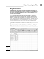
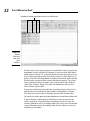
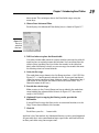
Excel displays the Advanced Filter dialog box, as shown in Figure 1-17.
Figure 1-17:
Set up an
advanced
filter here.
3. Tell Excel where to place the filtered table.
Use either Action radio button to specify whether you want the table filtered in place or copied to some new location. You can either filter the
table in place (meaning Excel just hides the records in the table that
don’t meet the filtering criteria), or you can copy the records that meet
the filtering criteria to a new location.
4. Verify the list range.
The worksheet range shown in the List Range text box — $A$1:$E$10 in
Figure 1-17 — should correctly identify the list. If your text box doesn’t
show the correct worksheet range, however, enter it. (Remember how I
said earlier in the chapter that Excel used to call these tables “lists”?
Hence the name of this box.)
5. Provide the criteria range.
Make an entry in the Criteria Range text box to identify the worksheet
range holding the advanced filter criteria. In Figure 1-17, the criteria
range is $A$13:$B$15.
6. (Optional) If you’re copying the filtering results, provide the
destination.
If you tell Excel to copy the filter results to some new location, use the
Copy To text box to identify this location.
7. Click OK.
Excel filters your list . . . I mean table.
And that’s that. Not too bad, eh? Advanced filtering is pretty straightforward.
All you really do is write some Boolean logic expressions and then tell Excel
to filter your table using those expressions.
29