1
Agilent Technologies E5500A/B
Phase Noise Measurement System
User’s Guide
Part number: E5500-90004
Printed in USA
June 2000
Supersedes September 1999
Revision A.01.05
Notice
The information contained in this document is subject to change without
notice.
Agilent Technologies makes no warranty of any kind with regard to this
material, including, but not limited to, the implied warranties of
merchantability and fitness for a particular purpose. Agilent Technologies
shall not be liable for errors contained herein or for incidental or
consequential damages in connection with the furnishing, performance, or
use of this material.
Agilent Technologies assumes no responsibility for the use or reliability of
its software on equipment that is not furnished by Agilent Technologies.
This document contains proprietary information which is protected by
copyright. All rights are reserved. No part of this document may be
photocopied, reproduced, or translated to another language without prior
written consent of Agilent Technologies Company.
U.S. Government Restricted Rights
The Software and documentation are provided with "Restricted Rights".
Use,duplication or disclosure by the U.S. Government is subject to the
restrictions set forth in subparagraph (c)(1)(ii) of the Rights in Technical
Data and Computer Software clauses in DFARS 252.227-7013 or as set
forth in subparagraph (c)(1) and (2) of the Commercial Computer Software Restricted Rights clauses at 48 CFR 52.227-19, as applicable. The
Contractor for the Software is Agilent Technologies Company, 3000
Hanover Street, Palo Alto, California 94304.
Trademarks
Windows NT 4.0 is a U.S trademarks of Microsoft Corp.
Pentium is a U.S. trademark of Intel Corporation
© Copyright Agilent Technologies Company 1997, 1998, 1999, 2000
Agilent Technologies Company
Santa Rosa Systems Division
1400 Fountaingrove Parkway
Santa Rosa, CA 95403-1799, U.S.A.
ii Agilent Technologies E5500 Phase Noise Measurement System
Software License
Terms
The following terms govern your use of the enclosed software programs
("Software") unless you have a separate written agreement with Agilent
Technologies.
License Grant
Agilent Technologies grants you a license to Use one copy of the version of
the Software identified in your documentation on any one product. "Use"
means storing, loading, installing,executing or displaying the Software. You
may not modify the Software or disable any licensing or control features of
the Software. Additional coppies of the software may be used for the sole
purpose of viewing previously measured data.
Ownership
The Software is owned and copyrighted by Agilent Technologies or its third
party licensors. Your license confers no title or ownership in the Software
and should not be construed as a sale of any rights in the Software. Agilent
Technologies' third party licensors may protect their rights in the event of
any violation of these terms.
Copies and Adaptations
You may only make copies or adaptations of the Software for archival
purposes or when copying or adaptation is an essential step in the authorized
Use of the Software
You must reproduce all copyright notices in the original Software on all
authorized copies or adaptations. You may not copy the Software onto any
bulletin board or similar system.
No Disassembly or Decryption
You may not disassemble, decompile or decrypt the Software unless Agilent
Technologies' prior written consent is obtained. In some jurisdictions,
Agilent Technologies' consent may not be required for disassembly or
decompilation. Upon request, you will provide Agilent Technologies with
reasonably detailed information regarding any disassembly or
decompilation.
Transfer
Your license will automatically terminate upon any transfer of the Software.
Upon transfer, you must deliver all copies of the Software and related
documentation to the transferee. The transferee must accept these License
Terms as a condition to the transfer.
Agilent Technologies E5500 Phase Noise Measurement System iii
Third Party Software
Software may include third party software. Those third parties may protect
their rights in the event of any violation of these License Terms.
Termination
Agilent Technologies may terminate your license upon notice forfailure to
comply with any of these License Terms. Upon termination, you must
immediately destroy the Software, together with all copies, adaptations and
merged portions in any form.
Export Requirements
You may not export or re-export the Software or any copy or adaptation in
violation of any applicable laws or regulations.
iv Agilent Technologies E5500 Phase Noise Measurement System
What You’ll Find in This Manual…
•
Chapter 1, “Getting Started with the Agilent Technologies E5500 Phase
Noise Measurement System”
•
Chapter 2, “Welcome to the HP E5500 Phase Noise Measurement
System Series of Solutions”
•
•
•
•
•
•
•
•
•
•
•
•
•
•
•
•
•
•
•
•
Chapter 3, “Your First Measurement”
Chapter 4, “Phase Noise Basics”
Chapter 5, “Expanding Your Measurement Experience”
Chapter 6, “Absolute Measurement Fundamentals”
Chapter 7, “Absolute Measurement Examples”
Chapter 8, “Residual Measurement Fundamentals”
Chapter 9, “Residual Measurement Examples”
Chapter 10, “FM Discriminator Fundamentals”
Chapter 11, “FM Discriminator Measurement Examples”
Chapter 12, “AM Noise Measurement Fundamentals”
Chapter 13, “AM Noise Measurement Examples”
Chapter 14, “Baseband Noise Measurement Examples”
Chapter 15, “Evaluating Your Measurement Results”
Chapter 16, “Advanced Software Features”
Chapter 17, “Error Messages and System Troubleshooting”
Chapter 18, “Reference Graphs and Tables”
Chapter 19, “Connect Diagrams”
Chapter 20, “System Specifications”
Chapter 21, “Phase Noise Customer Support”
Appendix A, “Connector Care and Preventive Maintenance”
Agilent Technologies E5500 Phase Noise Measurement System v
Limited Warranty
Software
Agilent Technologies warrants that the software will perform substantially
in accordance with the written materials for a period of one (1) year from the
date of receipt.
Agilent Technologies does not warrant that the operation of the software will
be uninterrupted or error free. In the event that this software product fails to
execute its programming instructions during the warranty period, the
customer’s remedy shall be to return the media to Agilent Technologies for
replacement. Should Agilent Technologies be unable to replace the media
within a reasonable amount of time, Customer’s alternate remedy shall be a
refund of the purchase price upon return of all copies of the software.
Media
Agilent Technologies warrants the media upon which this product is
recorded to be free from defects in materials and workmanship under normal
use for a period of one (1) year from the date of purchase. In the event any
media prove to be defective during the warranty period, Customer’s remedy
shall be to return the media to Agilent Technologies for replacement. Should
Agilent Technologies be unable to replace the media within a reasonable
amount of time, Customer’s alternate remedy shall be a refund of the
purchase price upon return of the product and all copies.
Notice of Warranty
Claims
Customer shall notify Agilent Technologies in writing of any warranty claim
not later than thirty (30) days after the expiration of the warranty period.
Limitation of
Warranty
Agilent Technologies makes no other express warranty, whether written or
oral, with respect to this product.
Any implied warranty of merchantability or fitness is limited to one (1) year
duration of this written warranty.
This warranty gives specific legal rights, and Customer may also have rights
which vary which vary from state to state, or province to province.
Exclusive Remedies
The remedies provided above are Customer’s sole and exclusive remedies.
In no event shall Agilent Technologies be liable for any direct, indirect,
special, incidental, or consequential damages (including lost profit) whether
based on warranty, contract, tort, or any other legal theory.
Assistance
For assistance, call your local Agilent Technologies Sales and Service
Office (refer to “Service and Support” on page -vii).
vi Agilent Technologies E5500 Phase Noise Measurement System
Service and Support
Any adjustment, maintenance, or repair of this product must be performed
by qualified personnel. Contact your customer engineer through your local
Agilent Technologies Service Center. You can find a list of Agilent
Technologies Service Centers on the web at
http://www.agilent.com/find/tmdir.
If you do not have access to the Internet, one of these Agilent Technologies
centers can direct you to your nearest Agilent Technologies representative:
United States:
Agilent Technologies Company
Test and Measurement Call Center
PO Box 4026
Englewood, CO 80155-4026
(800) 452 4844 (toll-free in US)
Canada:
Agilent Technologies Canada Ltd.
5150 Spectrum Way
Mississauga, Ontario L4W 5G1
(905) 206 4725
Europe:
Agilent Technologies European Marketing Centre
Postbox 999
1180 AZ Amstelveen
The Netherlands
(31 20) 547 9900
Japan:
Yokogawa-Agilent Technologies Ltd.
Measurement Assistance Center
9-1, Takakura-Cho, Hachioji-Shi
Tokyo 192, Japan
(81) 426 56 7832
(81) 426 56 7840 (FAX)
Latin America:
Agilent Technologies Latin American Region
Headquarters
5200 Blue Lagoon Drive, 9th Floor
Miami, Florida 33126, U.S.A.
(305) 267 4245
(305) 267 4288 (FAX)
Australia/New
Zealand:
Agilent Technologies Australia Ltd.
31-41 Joseph Street
Blackburn, Victoria 3130
Australia
1 800 629 485 (toll-free)
Asia-Pacific:
Agilent Technologies Asia Pacific Ltd.
17-21/F Shell Tower, Times Square
1 Matheson Street, Causeway Bay
Hong Kong
(852) 2599 7777
(852) 2506 9285 (FAX)
Agilent Technologies E5500 Phase Noise Measurement System vii
Notice . . . . . . . . . . . . . . . . . . . . . . . . . . . . . . . . . . . . . . . . . . . . . . . . . . . . . ii
Software License Terms . . . . . . . . . . . . . . . . . . . . . . . . . . . . . . . . . . . . iii
What You’ll Find in This Manual… . . . . . . . . . . . . . . . . . . . . . . . . . . . . . . v
Limited Warranty . . . . . . . . . . . . . . . . . . . . . . . . . . . . . . . . . . . . . . . . . . . . vi
Software . . . . . . . . . . . . . . . . . . . . . . . . . . . . . . . . . . . . . . . . . . . . . . . . vi
Media . . . . . . . . . . . . . . . . . . . . . . . . . . . . . . . . . . . . . . . . . . . . . . . . . . vi
Notice of Warranty Claims . . . . . . . . . . . . . . . . . . . . . . . . . . . . . . . . . . vi
Limitation of Warranty . . . . . . . . . . . . . . . . . . . . . . . . . . . . . . . . . . . . . vi
Exclusive Remedies . . . . . . . . . . . . . . . . . . . . . . . . . . . . . . . . . . . . . . . vi
Assistance . . . . . . . . . . . . . . . . . . . . . . . . . . . . . . . . . . . . . . . . . . . . . . . vi
Service and Support . . . . . . . . . . . . . . . . . . . . . . . . . . . . . . . . . . . . . . . . . vii
1.
Getting Started with the Agilent Technologies E5500 Phase Noise
Measurement System
What You’ll Find in This Chapter… . . . . . . . . . . . . . . . . . . . . . . . . . . . . 1-1
Introduction . . . . . . . . . . . . . . . . . . . . . . . . . . . . . . . . . . . . . . . . . . . . . . . . 1-2
Training Guidelines . . . . . . . . . . . . . . . . . . . . . . . . . . . . . . . . . . . . . . . . . 1-3
2.
Welcome to the Agilent Technologies E5500 Phase Noise Measurement
System Series of Solutions
What You’ll Find in This Chapter… . . . . . . . . . . . . . . . . . . . . . . . . . . . . 2-1
Introducing the Graphical User Interface . . . . . . . . . . . . . . . . . . . . . . . . . 2-2
System Requirements . . . . . . . . . . . . . . . . . . . . . . . . . . . . . . . . . . . . . . . . 2-4
3.
Your First Measurement
What You’ll Find in This Chapter… . . . . . . . . . . . . . . . . . . . . . . . . . . . . 3-1
Designed to Meet Your Needs . . . . . . . . . . . . . . . . . . . . . . . . . . . . . . . . . 3-2
As You Begin . . . . . . . . . . . . . . . . . . . . . . . . . . . . . . . . . . . . . . . . . . . 3-2
As You Progress . . . . . . . . . . . . . . . . . . . . . . . . . . . . . . . . . . . . . . . . . 3-2
E5500 Operation; A Guided Tour . . . . . . . . . . . . . . . . . . . . . . . . . . . . . . 3-3
Required Equipment . . . . . . . . . . . . . . . . . . . . . . . . . . . . . . . . . . . . . . 3-3
How to Begin . . . . . . . . . . . . . . . . . . . . . . . . . . . . . . . . . . . . . . . . . . . 3-3
Starting the Measurement Software . . . . . . . . . . . . . . . . . . . . . . . . . . . . . 3-4
Making a Measurement . . . . . . . . . . . . . . . . . . . . . . . . . . . . . . . . . . . . . . 3-5
Beginning the Measurement . . . . . . . . . . . . . . . . . . . . . . . . . . . . . . . . 3-7
Connect Diagram Example . . . . . . . . . . . . . . . . . . . . . . . . . . . . . . . . 3-8
Making the Measurement . . . . . . . . . . . . . . . . . . . . . . . . . . . . . . . . . . 3-8
Sweep-Segments . . . . . . . . . . . . . . . . . . . . . . . . . . . . . . . . . . . . . . . . 3-9
Congratulations . . . . . . . . . . . . . . . . . . . . . . . . . . . . . . . . . . . . . . . . . 3-9
To Learn More . . . . . . . . . . . . . . . . . . . . . . . . . . . . . . . . . . . . . . . . . . 3-9
4.
Phase Noise Basics
What You’ll Find in This Chapter . . . . . . . . . . . . . . . . . . . . . . . . . . . . . . 4-1
What is Phase Noise? . . . . . . . . . . . . . . . . . . . . . . . . . . . . . . . . . . . . . . . . 4-2
5.
Expanding Your Measurement Experience
What You’ll Find in This Chapter . . . . . . . . . . . . . . . . . . . . . . . . . . . . . . 5-1
Starting the Measurement Software . . . . . . . . . . . . . . . . . . . . . . . . . . . . . 5-2
Using the Asset Manager to Add a Source . . . . . . . . . . . . . . . . . . . . . . . . 5-3
Agilent Technologies E5500 Phase Noise Measurement System -i
Using the Server Hardware Connections to Specify the Source . . . . . . . 5-8
Testing the Agilent/HP 8663A Internal/External 10 MHz . . . . . . . . . . 5-10
Defining the Measurement . . . . . . . . . . . . . . . . . . . . . . . . . . . . . . . 5-11
Selecting a Reference Source . . . . . . . . . . . . . . . . . . . . . . . . . . . . . 5-13
Selecting Loop Suppression Verification . . . . . . . . . . . . . . . . . . . . 5-14
Setup Considerations for the Agilent/HP 8663A
10 MHz Measurement . . . . . . . . . . . . . . . . . . . . . . . . . . . . . . . 5-14
Beginning the Measurement . . . . . . . . . . . . . . . . . . . . . . . . . . . . . . 5-16
Sweep-Segments . . . . . . . . . . . . . . . . . . . . . . . . . . . . . . . . . . . . . . . 5-28
Checking the Beatnote . . . . . . . . . . . . . . . . . . . . . . . . . . . . . . . . . . 5-28
Making the Measurement . . . . . . . . . . . . . . . . . . . . . . . . . . . . . . . . 5-29
Testing the Agilent/HP 8644B Internal/External 10 MHz . . . . . . . . . . 5-33
Defining the Measurement . . . . . . . . . . . . . . . . . . . . . . . . . . . . . . . 5-34
Selecting a Reference Source . . . . . . . . . . . . . . . . . . . . . . . . . . . . . 5-36
Selecting Loop Suppression Verification . . . . . . . . . . . . . . . . . . . . 5-37
Setup Considerations for the Agilent/HP 8663A
10 MHz Measurement . . . . . . . . . . . . . . . . . . . . . . . . . . . . . . . 5-37
Beginning the Measurement . . . . . . . . . . . . . . . . . . . . . . . . . . . . . . 5-39
Sweep-Segments . . . . . . . . . . . . . . . . . . . . . . . . . . . . . . . . . . . . . . . 5-51
Checking the Beatnote . . . . . . . . . . . . . . . . . . . . . . . . . . . . . . . . . . 5-51
Making the Measurement . . . . . . . . . . . . . . . . . . . . . . . . . . . . . . . . 5-52
Viewing Markers . . . . . . . . . . . . . . . . . . . . . . . . . . . . . . . . . . . . . . . . . . 5-56
Omitting Spurs . . . . . . . . . . . . . . . . . . . . . . . . . . . . . . . . . . . . . . . . . . . . 5-57
Displaying the Parameter Summary . . . . . . . . . . . . . . . . . . . . . . . . . . . 5-59
Exporting Measurement Results . . . . . . . . . . . . . . . . . . . . . . . . . . . . . . 5-60
Exporting Trace Data . . . . . . . . . . . . . . . . . . . . . . . . . . . . . . . . . . . 5-61
Exporting Spur Data . . . . . . . . . . . . . . . . . . . . . . . . . . . . . . . . . . . . 5-62
Exporting X-Y Data . . . . . . . . . . . . . . . . . . . . . . . . . . . . . . . . . . . . 5-63
6.
Absolute Measurement Fundamentals
What You’ll Find in This Chapter . . . . . . . . . . . . . . . . . . . . . . . . . . . . . . 6-1
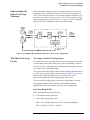
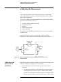
The Phase Lock Loop Technique . . . . . . . . . . . . . . . . . . . . . . . . . . . . . . 6-2
Understanding the Phase-Lock Loop Technique . . . . . . . . . . . . . . . 6-3
The Phase Lock Loop Circuit . . . . . . . . . . . . . . . . . . . . . . . . . . . . . . 6-3
What Sets the Measurement Noise Floor? . . . . . . . . . . . . . . . . . . . . . . . 6-6
The System Noise Floor . . . . . . . . . . . . . . . . . . . . . . . . . . . . . . . . . . 6-6
The Noise Level of the Reference Source . . . . . . . . . . . . . . . . . . . . 6-7
Selecting a Reference . . . . . . . . . . . . . . . . . . . . . . . . . . . . . . . . . . . . . . . 6-8
Using a Similar Device . . . . . . . . . . . . . . . . . . . . . . . . . . . . . . . . . . . 6-8
Using a Signal Generator . . . . . . . . . . . . . . . . . . . . . . . . . . . . . . . . . 6-9
Tuning Requirements . . . . . . . . . . . . . . . . . . . . . . . . . . . . . . . . . . . . 6-9
Estimating the Tuning Constant . . . . . . . . . . . . . . . . . . . . . . . . . . . . . . 6-11
Tracking Frequency Drift . . . . . . . . . . . . . . . . . . . . . . . . . . . . . . . . . . . 6-12
Evaluating Beatnote Drift . . . . . . . . . . . . . . . . . . . . . . . . . . . . . . . . 6-12
Changing the PTR . . . . . . . . . . . . . . . . . . . . . . . . . . . . . . . . . . . . . . . . . 6-14
The Tuning Qualifications . . . . . . . . . . . . . . . . . . . . . . . . . . . . . . . 6-14
Minimizing Injection Locking . . . . . . . . . . . . . . . . . . . . . . . . . . . . . . . . 6-16
-ii Agilent Technologies E5500 Phase Noise Measurement System
Adding Isolation . . . . . . . . . . . . . . . . . . . . . . . . . . . . . . . . . . . . . . . . 6-16
Increasing the PLL Bandwidth . . . . . . . . . . . . . . . . . . . . . . . . . . . . . 6-16
Inserting a Device . . . . . . . . . . . . . . . . . . . . . . . . . . . . . . . . . . . . . . . . . . 6-18
An Attenuator . . . . . . . . . . . . . . . . . . . . . . . . . . . . . . . . . . . . . . . . . . 6-18
An Amplifier . . . . . . . . . . . . . . . . . . . . . . . . . . . . . . . . . . . . . . . . . . 6-18
Evaluating Noise Above the Small Angle Line . . . . . . . . . . . . . . . . . . . 6-20
Determining the Phase Lock Loop Bandwidth . . . . . . . . . . . . . . . . 6-20
7.
Absolute Measurement Examples
What You’ll Find in This Chapter . . . . . . . . . . . . . . . . . . . . . . . . . . . . . . 7-1
Stable RF Oscillator . . . . . . . . . . . . . . . . . . . . . . . . . . . . . . . . . . . . . . . . . 7-2
Required Equipment . . . . . . . . . . . . . . . . . . . . . . . . . . . . . . . . . . . . . . 7-2
Defining the Measurement . . . . . . . . . . . . . . . . . . . . . . . . . . . . . . . . . 7-3
Selecting a Reference Source . . . . . . . . . . . . . . . . . . . . . . . . . . . . . . . 7-5
Selecting Loop Suppression Verification . . . . . . . . . . . . . . . . . . . . . . 7-6
Setup Considerations for the Stable RF Oscillator Measurement . . . 7-6
Beginning the Measurement . . . . . . . . . . . . . . . . . . . . . . . . . . . . . . . . 7-8
Checking the Beatnote . . . . . . . . . . . . . . . . . . . . . . . . . . . . . . . . . . . 7-19
Making the Measurement . . . . . . . . . . . . . . . . . . . . . . . . . . . . . . . . . 7-20
Free-Running RF Oscillator . . . . . . . . . . . . . . . . . . . . . . . . . . . . . . . . . . 7-24
Required Equipment . . . . . . . . . . . . . . . . . . . . . . . . . . . . . . . . . . . . . 7-24
Defining the Measurement . . . . . . . . . . . . . . . . . . . . . . . . . . . . . . . . 7-25
Selecting a Reference Source . . . . . . . . . . . . . . . . . . . . . . . . . . . . . . 7-27
Selecting Loop Suppression Verification . . . . . . . . . . . . . . . . . . . . . 7-28
Setup Considerations for the Free-Running RF
Oscillator Measurement . . . . . . . . . . . . . . . . . . . . . . . . . . . . . . . 7-28
Beginning the Measurement . . . . . . . . . . . . . . . . . . . . . . . . . . . . . . . 7-31
Checking the Beatnote . . . . . . . . . . . . . . . . . . . . . . . . . . . . . . . . . . . 7-42
Making the Measurement . . . . . . . . . . . . . . . . . . . . . . . . . . . . . . . . . 7-44
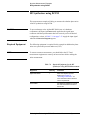
RF Synthesizer using DCFM . . . . . . . . . . . . . . . . . . . . . . . . . . . . . . . . . 7-48
Required Equipment . . . . . . . . . . . . . . . . . . . . . . . . . . . . . . . . . . . . . 7-48
Defining the Measurement . . . . . . . . . . . . . . . . . . . . . . . . . . . . . . . . 7-49
Selecting a Reference Source . . . . . . . . . . . . . . . . . . . . . . . . . . . . . . 7-51
Selecting Loop Suppression Verification . . . . . . . . . . . . . . . . . . . . . 7-52
Setup Considerations for the RF Synthesizer using
DCFM Measurement . . . . . . . . . . . . . . . . . . . . . . . . . . . . . . . . . 7-52
Beginning the Measurement . . . . . . . . . . . . . . . . . . . . . . . . . . . . . . . 7-55
Checking the Beatnote . . . . . . . . . . . . . . . . . . . . . . . . . . . . . . . . . . . 7-66
Making the Measurement . . . . . . . . . . . . . . . . . . . . . . . . . . . . . . . . . 7-68
RF Synthesizer using EFC . . . . . . . . . . . . . . . . . . . . . . . . . . . . . . . . . . . 7-72
Required Equipment . . . . . . . . . . . . . . . . . . . . . . . . . . . . . . . . . . . . . 7-72
Defining the Measurement . . . . . . . . . . . . . . . . . . . . . . . . . . . . . . . . 7-73
Selecting a Reference Source . . . . . . . . . . . . . . . . . . . . . . . . . . . . . . 7-75
Selecting Loop Suppression Verification . . . . . . . . . . . . . . . . . . . . . 7-76
Selecting a Reference Source . . . . . . . . . . . . . . . . . . . . . . . . . . . . . . 7-77
Setup Considerations for the RF Synthesizer using
EFC Measurement . . . . . . . . . . . . . . . . . . . . . . . . . . . . . . . . . . . 7-77
Agilent Technologies E5500 Phase Noise Measurement System -iii
Beginning the Measurement . . . . . . . . . . . . . . . . . . . . . . . . . . . . . . 7-80
Checking the Beatnote . . . . . . . . . . . . . . . . . . . . . . . . . . . . . . . . . . 7-91
Making the Measurement . . . . . . . . . . . . . . . . . . . . . . . . . . . . . . . . 7-93
Microwave Source . . . . . . . . . . . . . . . . . . . . . . . . . . . . . . . . . . . . . . . . . 7-97
Required Equipment . . . . . . . . . . . . . . . . . . . . . . . . . . . . . . . . . . . . 7-97
Defining the Measurement . . . . . . . . . . . . . . . . . . . . . . . . . . . . . . . 7-98
Selecting a Reference Source . . . . . . . . . . . . . . . . . . . . . . . . . . . . 7-100
Selecting Loop Suppression Verification . . . . . . . . . . . . . . . . . . . 7-101
Setup Considerations for the Microwave Source Measurement . . 7-101
Beginning the Measurement . . . . . . . . . . . . . . . . . . . . . . . . . . . . . 7-103
Checking the Beatnote . . . . . . . . . . . . . . . . . . . . . . . . . . . . . . . . . 7-110
Making the Measurement . . . . . . . . . . . . . . . . . . . . . . . . . . . . . . . 7-112
8.
Residual Measurement Fundamentals
What You’ll Find in This Chapter . . . . . . . . . . . . . . . . . . . . . . . . . . . . . . 8-1
What is Residual Noise? . . . . . . . . . . . . . . . . . . . . . . . . . . . . . . . . . . . . . 8-2
The Noise Mechanisms . . . . . . . . . . . . . . . . . . . . . . . . . . . . . . . . . . . 8-2
Basic Assumptions Regarding Residual Phase Noise Measurements . . . 8-4
Frequency Translation Devices . . . . . . . . . . . . . . . . . . . . . . . . . . . . . 8-4
Calibrating the Measurement . . . . . . . . . . . . . . . . . . . . . . . . . . . . . . . . . . 8-6
Calibration and Measurement Guidelines . . . . . . . . . . . . . . . . . . . . . 8-6
The Calibration Options . . . . . . . . . . . . . . . . . . . . . . . . . . . . . . . . . . . . . 8-9
User Entry of Phase Detector Constant . . . . . . . . . . . . . . . . . . . . . . . 8-9
Measured +/- DC Peak Voltage . . . . . . . . . . . . . . . . . . . . . . . . . . . . 8-13
Measured Beatnote . . . . . . . . . . . . . . . . . . . . . . . . . . . . . . . . . . . . . 8-16
Procedure . . . . . . . . . . . . . . . . . . . . . . . . . . . . . . . . . . . . . . . . . . . . 8-17
Synthesized Residual Measurement using Beatnote Cal . . . . . . . . 8-19
Procedure . . . . . . . . . . . . . . . . . . . . . . . . . . . . . . . . . . . . . . . . . . . . 8-19
Double-Sided Spur . . . . . . . . . . . . . . . . . . . . . . . . . . . . . . . . . . . . . 8-21
Single-Sided Spur . . . . . . . . . . . . . . . . . . . . . . . . . . . . . . . . . . . . . . 8-24
Measurement Difficulties . . . . . . . . . . . . . . . . . . . . . . . . . . . . . . . . . . . 8-28
System Connections . . . . . . . . . . . . . . . . . . . . . . . . . . . . . . . . . . . . 8-28
9.
Residual Measurement Examples
What You’ll Find in This Chapter . . . . . . . . . . . . . . . . . . . . . . . . . . . . . . 9-1
Amplifier Measurement Example . . . . . . . . . . . . . . . . . . . . . . . . . . . . . . 9-2
Required Equipment . . . . . . . . . . . . . . . . . . . . . . . . . . . . . . . . . . . . . 9-2
Defining the Measurement . . . . . . . . . . . . . . . . . . . . . . . . . . . . . . . . 9-3
Setup Considerations . . . . . . . . . . . . . . . . . . . . . . . . . . . . . . . . . . . . . 9-7
Beginning the Measurement . . . . . . . . . . . . . . . . . . . . . . . . . . . . . . . 9-7
Making the Measurement . . . . . . . . . . . . . . . . . . . . . . . . . . . . . . . . 9-10
When the Measurement is Complete . . . . . . . . . . . . . . . . . . . . . . . 9-13
10.
FM Discriminator Fundamentals
What You’ll Find in This Chapter . . . . . . . . . . . . . . . . . . . . . . . . . . . . .
The Frequency Discriminator Method . . . . . . . . . . . . . . . . . . . . . . . . .
Basic Theory . . . . . . . . . . . . . . . . . . . . . . . . . . . . . . . . . . . . . . . . . .
The Discriminator Transfer Response . . . . . . . . . . . . . . . . . . . . . .
-iv Agilent Technologies E5500 Phase Noise Measurement System
10-1
10-2
10-2
10-3
11.
FM Discriminator Measurement Examples
What You’ll Find in This Chapter . . . . . . . . . . . . . . . . . . . . . . . . . . . . . 11-1
Introduction . . . . . . . . . . . . . . . . . . . . . . . . . . . . . . . . . . . . . . . . . . . . . . . 11-2
FM Discriminator Measurement using Double-Sided Spur Calibration 11-3
Required Equipment . . . . . . . . . . . . . . . . . . . . . . . . . . . . . . . . . . . . . 11-3
Determining the Discriminator
(Delay Line) Length . . . . . . . . . . . . . . . . . . . . . . . . . . . . . . . . . . 11-4
Defining the Measurement . . . . . . . . . . . . . . . . . . . . . . . . . . . . . . . . 11-5
Setup Considerations . . . . . . . . . . . . . . . . . . . . . . . . . . . . . . . . . . . . 11-9
Beginning the Measurement . . . . . . . . . . . . . . . . . . . . . . . . . . . . . . 11-10
Making the Measurement . . . . . . . . . . . . . . . . . . . . . . . . . . . . . . . . 11-13
When the Measurement is Complete . . . . . . . . . . . . . . . . . . . . . . . 11-15
Discriminator Measurement using FM Rate
and Deviation Calibration . . . . . . . . . . . . . . . . . . . . . . . . . . . . . . . 11-18
Required Equipment . . . . . . . . . . . . . . . . . . . . . . . . . . . . . . . . . . . . 11-18
Determining the Discriminator (Delay Line) Length . . . . . . . . . . . 11-19
Defining the Measurement . . . . . . . . . . . . . . . . . . . . . . . . . . . . . . . 11-20
Setup Considerations . . . . . . . . . . . . . . . . . . . . . . . . . . . . . . . . . . . 11-24
Beginning the Measurement . . . . . . . . . . . . . . . . . . . . . . . . . . . . . . 11-25
Making the Measurement . . . . . . . . . . . . . . . . . . . . . . . . . . . . . . . . 11-28
When the Measurement is Complete . . . . . . . . . . . . . . . . . . . . . . . 11-30
12.
AM Noise Measurement Fundamentals
What You’ll Find in This Chapter . . . . . . . . . . . . . . . . . . . . . . . . . . . . . 12-1
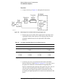
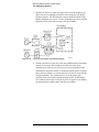
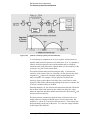
AM-Noise Measurement Theory of Operation . . . . . . . . . . . . . . . . . . . . 12-2
Basic Noise Measurement . . . . . . . . . . . . . . . . . . . . . . . . . . . . . . . . 12-2
Phase Noise Measurement . . . . . . . . . . . . . . . . . . . . . . . . . . . . . . . . 12-2
Amplitude Noise Measurement . . . . . . . . . . . . . . . . . . . . . . . . . . . . . . . 12-3
AM Noise Measurement Block Diagrams . . . . . . . . . . . . . . . . . . . . 12-3
AM Detector . . . . . . . . . . . . . . . . . . . . . . . . . . . . . . . . . . . . . . . . . . . 12-4
Calibration and Measurement General Guidelines . . . . . . . . . . . . . . . . . 12-6
Method 1:
User Entry of Phase Detector Constant . . . . . . . . . . . . . . . . . . . . . . 12-8
Method 1, example 1 . . . . . . . . . . . . . . . . . . . . . . . . . . . . . . . . . . . . 12-8
Method 1, Example 2 . . . . . . . . . . . . . . . . . . . . . . . . . . . . . . . . . . . 12-10
Method 2: Double-Sided Spur . . . . . . . . . . . . . . . . . . . . . . . . . . . . . . . 12-12
Method 2, Example 1 . . . . . . . . . . . . . . . . . . . . . . . . . . . . . . . . . . . 12-12
Method 2, Example 2 . . . . . . . . . . . . . . . . . . . . . . . . . . . . . . . . . . . 12-14
Method 3: Single-Sided-Spur . . . . . . . . . . . . . . . . . . . . . . . . . . . . . . . . 12-17
13.
AM Noise Measurement Examples
What You’ll Find in This Chapter . . . . . . . . . . . . . . . . . . . . . . . . . . . . . 13-1
AM Noise using an Agilent/HP 70420A Option 001 . . . . . . . . . . . . . . . 13-2
Defining the Measurement . . . . . . . . . . . . . . . . . . . . . . . . . . . . . . . . 13-3
Beginning the Measurement . . . . . . . . . . . . . . . . . . . . . . . . . . . . . . . 13-7
Making the Measurement . . . . . . . . . . . . . . . . . . . . . . . . . . . . . . . . . 13-9
When the Measurement is Complete . . . . . . . . . . . . . . . . . . . . . . . . 13-9
Agilent Technologies E5500 Phase Noise Measurement System -v
14.
Baseband Noise Measurement Examples
What You’ll Find in This Chapter . . . . . . . . . . . . . . . . . . . . . . . . . . . . .
Baseband Noise using a Test Set Measurement Example . . . . . . . . . . .
Defining the Measurement . . . . . . . . . . . . . . . . . . . . . . . . . . . . . . .
Beginning the Measurement . . . . . . . . . . . . . . . . . . . . . . . . . . . . . .
Making the Measurement . . . . . . . . . . . . . . . . . . . . . . . . . . . . . . . .
Baseband Noise without using a Test Set Measurement Example . . . .
Defining the Measurement . . . . . . . . . . . . . . . . . . . . . . . . . . . . . . .
Beginning the Measurement . . . . . . . . . . . . . . . . . . . . . . . . . . . . . .
Making the Measurement . . . . . . . . . . . . . . . . . . . . . . . . . . . . . . . .
15.
14-1
14-2
14-2
14-3
14-4
14-6
14-6
14-7
14-7
Evaluating Your Measurement Results
What You’ll Find in This Chapter . . . . . . . . . . . . . . . . . . . . . . . . . . . . . 15-1
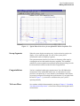
Evaluating the Results . . . . . . . . . . . . . . . . . . . . . . . . . . . . . . . . . . . . . . 15-2
Looking For Obvious Problems . . . . . . . . . . . . . . . . . . . . . . . . . . . 15-2
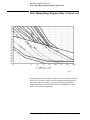
Comparing Against Expected Data . . . . . . . . . . . . . . . . . . . . . . . . . 15-3
Gathering More Data . . . . . . . . . . . . . . . . . . . . . . . . . . . . . . . . . . . . . . . 15-6
Repeating the Measurement . . . . . . . . . . . . . . . . . . . . . . . . . . . . . . 15-6
Doing More Research . . . . . . . . . . . . . . . . . . . . . . . . . . . . . . . . . . . 15-6
Outputting the Results . . . . . . . . . . . . . . . . . . . . . . . . . . . . . . . . . . . . . . 15-7
Using a Printer . . . . . . . . . . . . . . . . . . . . . . . . . . . . . . . . . . . . . . . . 15-7
Graph of Results . . . . . . . . . . . . . . . . . . . . . . . . . . . . . . . . . . . . . . . . . . 15-8
Marker . . . . . . . . . . . . . . . . . . . . . . . . . . . . . . . . . . . . . . . . . . . . . . . 15-9
Omit Spurs . . . . . . . . . . . . . . . . . . . . . . . . . . . . . . . . . . . . . . . . . . 15-10
Parameter Summary . . . . . . . . . . . . . . . . . . . . . . . . . . . . . . . . . . . 15-12
Problem Solving . . . . . . . . . . . . . . . . . . . . . . . . . . . . . . . . . . . . . . . . . 15-13
Discontinuity in the Graph . . . . . . . . . . . . . . . . . . . . . . . . . . . . . . 15-14
Higher Noise Level . . . . . . . . . . . . . . . . . . . . . . . . . . . . . . . . . . . . 15-15
Spurs on the Graph . . . . . . . . . . . . . . . . . . . . . . . . . . . . . . . . . . . . 15-20
Small Angle Line . . . . . . . . . . . . . . . . . . . . . . . . . . . . . . . . . . . . . 15-22
16.
Advanced Software Features
What You’ll Find in This Chapter… . . . . . . . . . . . . . . . . . . . . . . . . . . . 16-1
Introduction . . . . . . . . . . . . . . . . . . . . . . . . . . . . . . . . . . . . . . . . . . . . . . 16-2
Phase Lock Loop Suppression . . . . . . . . . . . . . . . . . . . . . . . . . . . . . . . . 16-3
PLL Suppression Parameters . . . . . . . . . . . . . . . . . . . . . . . . . . . . . . . . . 16-3
Ignore Out Of Lock Mode . . . . . . . . . . . . . . . . . . . . . . . . . . . . . . . . . . . 16-6
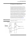
PLL Suppression Verification Process . . . . . . . . . . . . . . . . . . . . . . . . . 16-7
PLL Suppression Information . . . . . . . . . . . . . . . . . . . . . . . . . . . . . 16-8
PLL Gain Change . . . . . . . . . . . . . . . . . . . . . . . . . . . . . . . . . . . . . .16-12
Maximum Error . . . . . . . . . . . . . . . . . . . . . . . . . . . . . . . . . . . . . . . 16-12
Accuracy Degradation . . . . . . . . . . . . . . . . . . . . . . . . . . . . . . . . . . 16-12
Supporting an Embedded VXI PC: . . . . . . . . . . . . . . . . . . . . . . . . 16-12
Blanking Frequency and Amplitude Information on the Phase Noise Graph
16-13
Security Level Procedure . . . . . . . . . . . . . . . . . . . . . . . . . . . . . . . 16-13
-vi Agilent Technologies E5500 Phase Noise Measurement System
17.
Error Messages and System Troubleshooting
What You’ll Find in This Chapter . . . . . . . . . . . . . . . . . . . . . . . . . . . . . 17-1
18.
Reference Graphs and Tables
Graphs and Tables You’ll Find in This Chapter . . . . . . . . . . . . . . . . . . . 18-1
Graphs . . . . . . . . . . . . . . . . . . . . . . . . . . . . . . . . . . . . . . . . . . . . . . . 18-1
Tables . . . . . . . . . . . . . . . . . . . . . . . . . . . . . . . . . . . . . . . . . . . . . . . . 18-1
Approximate System Phase Noise Floor vs. R Port Signal Level . . . . . 18-2
Phase Noise Floor and Region of Validity . . . . . . . . . . . . . . . . . . . . . . . 18-3
Phase Noise Level of Various Agilent/HP Sources . . . . . . . . . . . . . . . . 18-4
Increase in Measured Noise as Ref Source Approaches UUT Noise . . . 18-5
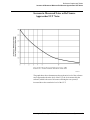
Approximate Sensitivity of Delay Line Discriminator . . . . . . . . . . . . . . 18-6
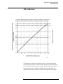
AM Calibration . . . . . . . . . . . . . . . . . . . . . . . . . . . . . . . . . . . . . . . . . . . . 18-7
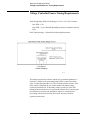
Voltage Controlled Source Tuning Requirements . . . . . . . . . . . . . . . . . 18-8
Tune Range of VCO vs. Center Voltage . . . . . . . . . . . . . . . . . . . . . . . . 18-9
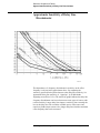
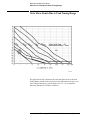
Peak Tuning Range Required Due to Noise Level . . . . . . . . . . . . . . . . 18-10
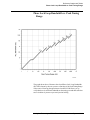
Phase Lock Loop Bandwidth vs. Peak Tuning Range . . . . . . . . . . . . . 18-11
Noise Floor Limits Due to Peak Tuning Range . . . . . . . . . . . . . . . . . . 18-12
Tuning Characteristics of Various VCO Source Options . . . . . . . . . . . 18-13
Agilent/HP 8643A Frequency Limits . . . . . . . . . . . . . . . . . . . . . . . . . . 18-14
Agilent/HP 8643A Mode Keys . . . . . . . . . . . . . . . . . . . . . . . . . . . 18-14
How to Access Special Functions . . . . . . . . . . . . . . . . . . . . . . . . . 18-15
Description of Special Functions 120 and 125 . . . . . . . . . . . . . . . . 18-15
Agilent/HP 8644B Frequency Limits . . . . . . . . . . . . . . . . . . . . . . . . . . 18-16
Agilent/HP 8644B Mode Keys . . . . . . . . . . . . . . . . . . . . . . . . . . . 18-16
How to Access Special Functions . . . . . . . . . . . . . . . . . . . . . . . . . 18-17
Description of Special Function 120 . . . . . . . . . . . . . . . . . . . . . . . 18-17
Agilent/HP 8664A Frequency Limits . . . . . . . . . . . . . . . . . . . . . . . . . . 18-18
Agilent/HP 8664A Mode Keys . . . . . . . . . . . . . . . . . . . . . . . . . . . 18-18
How to Access Special Functions . . . . . . . . . . . . . . . . . . . . . . . . . 18-19
Description of Special Functions 120 . . . . . . . . . . . . . . . . . . . . . . 18-19
Agilent/HP 8665A Frequency Limits . . . . . . . . . . . . . . . . . . . . . . . . . . 18-20
Agilent/HP 8665A Mode Keys . . . . . . . . . . . . . . . . . . . . . . . . . . . 18-20
How to Access Special Functions . . . . . . . . . . . . . . . . . . . . . . . . . 18-21
Description of Special Functions 120 and 124 . . . . . . . . . . . . . . . . 18-21
Agilent/HP 8665B Frequency Limits . . . . . . . . . . . . . . . . . . . . . . . . . . 18-22
Agilent/HP 8665B Mode Keys . . . . . . . . . . . . . . . . . . . . . . . . . . . 18-22
How to Access Special Functions . . . . . . . . . . . . . . . . . . . . . . . . . 18-23
Description of Special Functions 120 and 124 . . . . . . . . . . . . . . . . 18-23
19.
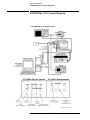
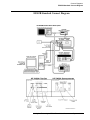
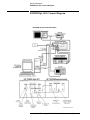
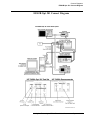
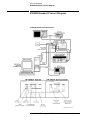
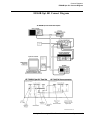
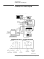
Connect Diagrams
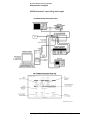
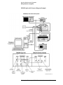
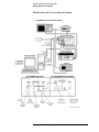
Connect Diagrams You’ll Find in This Chapter . . . . . . . . . . . . . . . . . . . 19-1
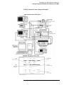
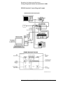
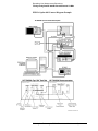
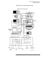
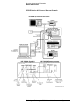
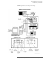
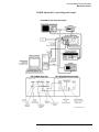
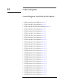
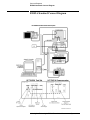
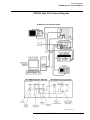
E5501A Standard Connect Diagram . . . . . . . . . . . . . . . . . . . . . . . . . . . . 19-2
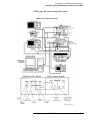
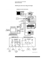
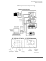
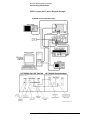
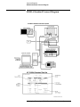
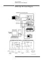
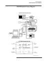
E5501A Opt. 001 Connect Diagram . . . . . . . . . . . . . . . . . . . . . . . . . . . . 19-3
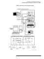
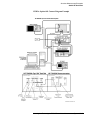
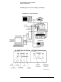
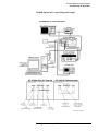
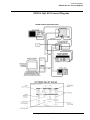
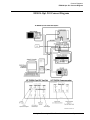
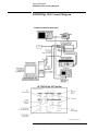
E5501A Opt. 201, 430, 440 Connect Diagram . . . . . . . . . . . . . . . . . . . . 19-4
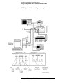
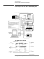
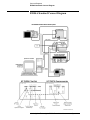
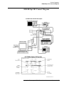
E5501A Opt. 201 Connect Diagram . . . . . . . . . . . . . . . . . . . . . . . . . . . . 19-5
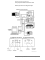
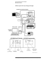
E5502A Standard Connect Diagram . . . . . . . . . . . . . . . . . . . . . . . . . . . . 19-6
Agilent Technologies E5500 Phase Noise Measurement System -vii
E5502A Opt. 001 Connect Diagram
E5502A Opt. 201 Connect Diagram
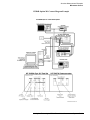
E5503A Standard Connect Diagram
E5503A Opt. 001 Connect Diagram
E5503A Opt. 201 Connect Diagram
E5504A Standard Connect Diagram
E5504A Opt. 001 Connect Diagram
E5504A Opt. 201 Connect Diagram
E5501B Standard Connect Diagram
E5501B Opt. 001 Connect Diagram
E5501B Opt. 201 Connect Diagram
E5502B Standard Connect Diagram
E5502B Opt. 001 Connect Diagram
E5502B Opt. 201 Connect Diagram
E5503B Standard Connect Diagram
E5503B Opt. 001 Connect Diagram
E5503B Opt. 201 Connect Diagram
E5504B Standard Connect Diagram
E5504B Opt. 001 Connect Diagram
E5504B Opt. 201 Connect Diagram
20.
. . . . . . . . . . . . . . . . . . . . . . . . . . . 19-7
. . . . . . . . . . . . . . . . . . . . . . . . . . . 19-8
. . . . . . . . . . . . . . . . . . . . . . . . . . . 19-9
. . . . . . . . . . . . . . . . . . . . . . . . . . 19-10
. . . . . . . . . . . . . . . . . . . . . . . . . . 19-11
. . . . . . . . . . . . . . . . . . . . . . . . . . 19-12
. . . . . . . . . . . . . . . . . . . . . . . . . . 19-13
. . . . . . . . . . . . . . . . . . . . . . . . . . 19-14
. . . . . . . . . . . . . . . . . . . . . . . . . . 19-15
. . . . . . . . . . . . . . . . . . . . . . . . . . 19-16
. . . . . . . . . . . . . . . . . . . . . . . . . . 19-17
. . . . . . . . . . . . . . . . . . . . . . . . . . 19-18
. . . . . . . . . . . . . . . . . . . . . . . . . . 19-19
. . . . . . . . . . . . . . . . . . . . . . . . . . 19-20
. . . . . . . . . . . . . . . . . . . . . . . . . . 19-21
. . . . . . . . . . . . . . . . . . . . . . . . . . 19-22
. . . . . . . . . . . . . . . . . . . . . . . . . . 19-23
. . . . . . . . . . . . . . . . . . . . . . . . . . 19-24
. . . . . . . . . . . . . . . . . . . . . . . . . . 19-25
. . . . . . . . . . . . . . . . . . . . . . . . . . 19-26
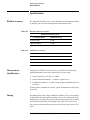
System Specifications
What You’ll Find in This Chapter… . . . . . . . . . . . . . . . . . . . . . . . . . . .
Specifications . . . . . . . . . . . . . . . . . . . . . . . . . . . . . . . . . . . . . . . . . . . . .
Reliable Accuracy . . . . . . . . . . . . . . . . . . . . . . . . . . . . . . . . . . . . . .
Measurement Qualifications . . . . . . . . . . . . . . . . . . . . . . . . . . . . . .
Tuning . . . . . . . . . . . . . . . . . . . . . . . . . . . . . . . . . . . . . . . . . . . . . . .
21.
20-1
20-2
20-2
20-2
20-2
Phase Noise Customer Support
What You’ll Find in This Chapter . . . . . . . . . . . . . . . . . . . . . . . . . . . . . 21-1
Software and Documentation Updates . . . . . . . . . . . . . . . . . . . . . . . . . 21-2
Contacting Customer Support . . . . . . . . . . . . . . . . . . . . . . . . . . . . . . . . 21-3
22.
Connector Care and
Preventive Maintenance
What You’ll Find in This Appendix… . . . . . . . . . . . . . . . . . . . . . . . . . . A-1
Using, Inspecting, and Cleaning RF Connectors . . . . . . . . . . . . . . . . . . . A-2
Repeatability . . . . . . . . . . . . . . . . . . . . . . . . . . . . . . . . . . . . . . . . . . . A-2
RF Cable and Connector Care . . . . . . . . . . . . . . . . . . . . . . . . . . . . . A-3
Proper Connector Torque . . . . . . . . . . . . . . . . . . . . . . . . . . . . . . . . . A-3
Connector Wear and Damage . . . . . . . . . . . . . . . . . . . . . . . . . . . . . . A-4
SMA Connector Precautions . . . . . . . . . . . . . . . . . . . . . . . . . . . . . . . A-4
Cleaning Procedure . . . . . . . . . . . . . . . . . . . . . . . . . . . . . . . . . . . . . . A-4
Removing and Reinstalling Instruments . . . . . . . . . . . . . . . . . . . . . . . . . A-6
General Procedures and Techniques . . . . . . . . . . . . . . . . . . . . . . . . . A-6
GPIB Connectors . . . . . . . . . . . . . . . . . . . . . . . . . . . . . . . . . . . . . . . A-8
Precision 2.4 mm and 3.5 mm Connectors . . . . . . . . . . . . . . . . . . . . A-8
Bent Semirigid Cables . . . . . . . . . . . . . . . . . . . . . . . . . . . . . . . . . . . A-9
-viii Agilent Technologies E5500 Phase Noise Measurement System
Other Multipin Connectors . . . . . . . . . . . . . . . . . . . . . . . . . . . . . . . . A-9
MMS Module Removal and Reinstallation . . . . . . . . . . . . . . . . . . A-11
Touch-Up Paint . . . . . . . . . . . . . . . . . . . . . . . . . . . . . . . . . . . . . . . . . . . A-12
Agilent Technologies E5500 Phase Noise Measurement System -ix
1
Getting Started with the Agilent
Technologies E5500 Phase Noise
Measurement System
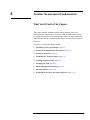
What You’ll Find in This Chapter…
•
•
Introduction, page 1-2
Training Guidelines, page 1-3
Agilent Technologies E5500 Phase Noise Measurement System 1-1
Getting Started with the Agilent Technologies E5500 Phase Noise
Measurement System
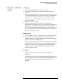
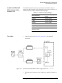
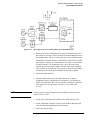
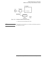
Introduction
The table on the right-hand page (Training Guidelines, page 1-3) will help
you first learn about, then use the E5500 phase noise measurement system.
The following three areas are covered in this manual:
•
•
•
Leaning about the E5500 phase noise measurement system
Learning about phase noise basics and measurement fundamentals.
Using the phase noise measurement system to make specific phase noise
measurements.
NOTE
Installation information for your system is provided in the E5500
Installation Guide.
NOTE
For application assistance, contact you local Agilent Technologies sales
representative.
1-2 Agilent Technologies E5500 Phase Noise Measurement System
Getting Started with the Agilent Technologies E5500 Phase Noise
Measurement System
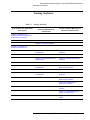
Training Guidelines
Table 1-1
Learning about the E5500 Phase
Noise System
Training Guidelines
Learning about Phase Noise
Basics and Measurement
Fundamentals
Using the E5500 to Make Specific
Phase Noise Measurements
Chapter 2, “Welcome to the
E5500 Phase Noise Measurement
System Series of Solutions”
Chapter 3, “Your First Measurement”
Chapter 4, “Phase Noise Basics”
Chapter 5, “Expanding Your
Measurement Experience”
Chapter 6, “Absolute Measurement
Fundamentals”
Chapter 7, “Absolute Measurement
Examples”
Chapter 8, “Residual Measurement
Fundamentals”
Chapter 9, “Residual Measurement
Examples”
Chapter 10, “FM Discriminator
Fundamentals”
Chapter 11, “FM Discriminator
Measurement Examples”
Chapter 12, “AM Noise Measurement
Fundamentals”
Chapter 13, “AM Noise Measurement
Examples”
Chapter 14, “Baseband Noise
Measurement Examples”
Chapter 15, “Evaluating Your
Measurement Results”
Chapter 16, “Advanced Software
Features”
Chapter 17, “Error Messages and
System Troubleshooting”
Chapter 18, “Reference Graphs and
Tables”
Agilent Technologies E5500 Phase Noise Measurement System 1-3
2
Welcome to the Agilent Technologies E5500
Phase Noise Measurement System Series of
Solutions
What You’ll Find in This Chapter…
•
•
Introducing the Graphical User Interface, page 2-2
System Requirements, page 2-4
Agilent Technologies E5500 Phase Noise Measurement System 2-1
Welcome to the Agilent Technologies E5500 Phase Noise Measurement
System Series of Solutions
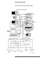
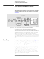
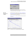
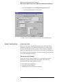
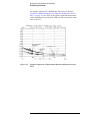
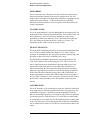
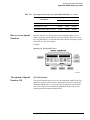
Introducing the Graphical User Interface
The graphical user interface gives the user instant access to all measurement
functions making it easy to configure a system and define or initiate
measurements. The most frequently used functions are displayed as icons on
a toolbar, allowing quick and easy access to the measurement information.
The forms-based graphical interaction helps you define your measurement
quickly and easily. Each form tab is labeled with its content, preventing you
from getting lost in the define process.
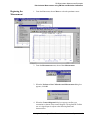
Three default segment tables are provided. To obtain a quick look at your
data, select the “fast” quality level. If more frequency resolution to separate
spurious signals is important, the ‘normal’ and “high resolution” quality
levels are available. If you need to customize the offset range beyond the
defaults provided, tailor the measurement segment tables to meet your needs
and save them as a “custom” selection.
You can place up to nine markers on the data trace, that can be plotted with
the measured data.
Other features include:
•
•
•
•
•
Plotting data without spurs
Tabular listing of spurs
Plotting in alternate bandwidths
Parameter summary
Color printouts to any supported color printer
2-2 Agilent Technologies E5500 Phase Noise Measurement System
Welcome to the Agilent Technologies E5500 Phase Noise Measurement
System Series of Solutions
Agilent Technologies E5500 Phase Noise Measurement System 2-3
Welcome to the Agilent Technologies E5500 Phase Noise Measurement
System Series of Solutions
System Requirements
In case you want a quick review of the system requirements, we have listed
them here.
The minimum system requirements for the phase noise measurement
software are:
•
•
•
•
•
•
•
•
Pentium microprocessor (100 MHz or higher recommended)
32 megabytes (MB) of memory (RAM)
1 gigabyte (GB) hard disk
Super Video Graphics Array (SVGA)
2 additional 16-bit ISA slots available for the phase noise system
hardware.
❍
1 for PC-Digitizer or VXI/MXI Interface
❍
1 for GPIB Interface Card
Windows NT 4.0
Windows NT 4.0 Service Pack 3
Agilent/HP 82341C GPIB Interface Card
2-4 Agilent Technologies E5500 Phase Noise Measurement System
3
Your First Measurement
What You’ll Find in This Chapter…
•
•
•
E5500 Operation; A Guided Tour, page 3-3
Starting the Measurement Software, page 3-4
Making a Measurement, page 3-5
Agilent Technologies E5500 Phase Noise Measurement System 3-1
Your First Measurement
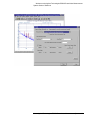
Designed to Meet Your Needs
Designed to Meet Your Needs
The Agilent E5500 phase noise measurement system is a high performance
measurement tool that enables you to fully evaluate the noise characteristics
of your electronic instruments and components with unprecedented speed
and ease. The phase noise measurement system provides you with the
flexibility needed to meet today’s broad range of noise measurement
requirements.
In order to use the phase noise system effectively, it is important that you
have a good understanding of the noise measurement you are making. This
manual is designed to help you gain that understanding and quickly progress
from a beginning user of the phase noise system to a proficient user of the
system’s basic measurement capabilities.
NOTE
If you have just received your system, or need help with connecting the
hardware or loading software, refer to Installation Guide now. Once you
have completed the installation procedures presented in Installation Guide,
return to the following page to begin learning how to make noise
measurements with the system.
As You Begin
The “E5500 Operation; A Guided Tour” contains a step-by-step procedure
for completing a phase noise measurement. This measurement
demonstration introduces system operating fundamentals for whatever type
of device you plan to measure.
Once you are familiar with the information in this chapter, you will be ready
to start Chapter 5, “Expanding Your Measurement Experience”. After you
have completed “Expanding Your Measurement Experience”, you will want
to refer to Chapter 15, “Evaluating Your Measurement Results” for help in
analyzing and verifying your test results.
As You Progress
As you become familiar with the operation of the phase noise system you
will need to refer to this guide less often. There may, however, be times
when you encounter problems while running your measurements. Problem
solving suggestions have been provided at the back of chapter 3 to help you
deal with conditions that can prevent the system from completing its
measurement.
3-2 Agilent Technologies E5500 Phase Noise Measurement System
Your First Measurement
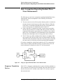
E5500 Operation; A Guided Tour
E5500 Operation; A Guided Tour
This measurement demonstration will introduce you to the system’s
operation by guiding you through an actual phase noise measurement.
You will be measuring the phase noise of the Agilent/HP 70420A test set’s
internal noise source. (The measurement made in this demonstration is the
same measurement that is made to verify the system’s operation.)
As you step through the measurement procedures, you will soon discover
that the phase noise measurement system offers enormous flexibility for
measuring the noise characteristics of your signal sources and two-port
devices.
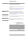
Required Equipment
The equipment shipped with this system is all that is required to complete
this demonstration. (Refer to the E5500 Installation Guide if you need
information about setting up the hardware or installing the software.)
How to Begin
Follow the set up procedures beginning on the next page. The phase noise
measurement system will display a setup diagram that shows you the correct
front panel cable connections to make for this measurement.
Agilent Technologies E5500 Phase Noise Measurement System 3-3
Your First Measurement
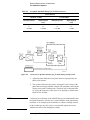
Starting the Measurement Software
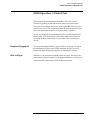
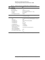
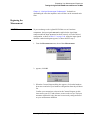
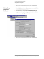
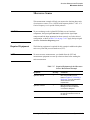
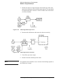
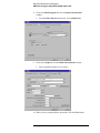
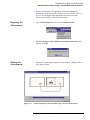
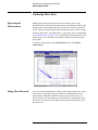
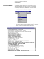
Starting the Measurement Software
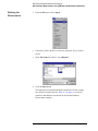
1. Place the E5500 phase noise measurement software disk in the disc
holder and insert in the CD-ROM drive.
2. Click the Start button, point to Programs, point to Agilent
Measurement Systems, point to E5500 Phase Noise, and then click
Measurement Client.
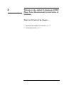
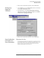
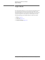
3. The following phase noise measurement subsystem dialog box appears.
Your dialog box may look slightly different.
3-4 Agilent Technologies E5500 Phase Noise Measurement System
Your First Measurement
Making a Measurement
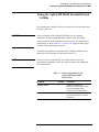
Making a Measurement
This first measurement is a confidence test that functionally checks the
Agilent/HP 70420A test set’s filters and low-noise amplifiers using the test
set’s internal noise source. The phase detectors are not tested. This
confidence test also confirms that the test set, PC, and analyzers are
communicating with each other.
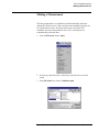
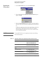
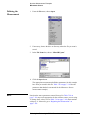
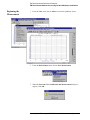
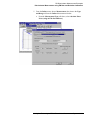
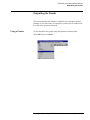
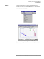
1. From the File menu, choose Open.
2. If necessary, choose the drive or directory where the file you want is
stored.
3. In the File Name box, choose Confidence.pnm.
Agilent Technologies E5500 Phase Noise Measurement System 3-5
Your First Measurement
Making a Measurement
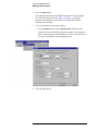
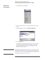
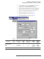
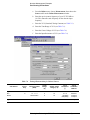
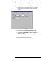
4. Click the Open button.
The appropriate measurement definition parameters for this example
have been pre-stored in this file. Table 3-1 on page 3-10 lists the
parameter data that has been entered for the Agilent/HP 70420A
confidence test example.
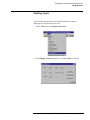
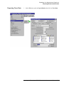
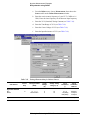
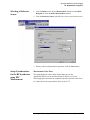
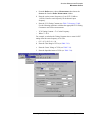
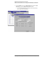
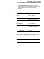
5. To view the parameter data in the software,
a. From the Define menu, choose Measurement; then choose the
Sources tab from the Define Measurement window. The parameter
data is entered using the tabbed windows. Select various tabs to see
the type of information entered behind each tab.
6. Click the Close button.
3-6 Agilent Technologies E5500 Phase Noise Measurement System
Your First Measurement
Making a Measurement
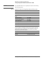
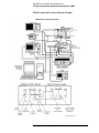
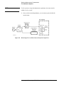
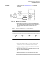
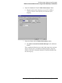
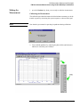
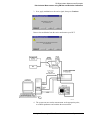
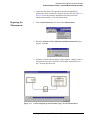
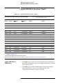
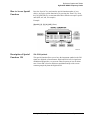
Beginning the
Measurement
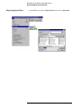
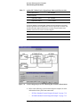
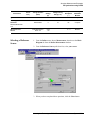
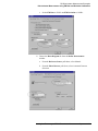
1. From the Measurement menu, choose New Measurement.
2. When the Do you want to Perform a New Calibration and
Measurement dialog box appears, click Yes.
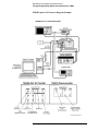
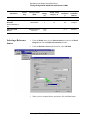
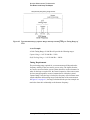
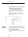
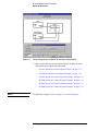
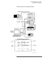
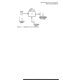
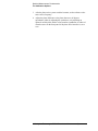
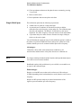
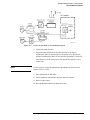
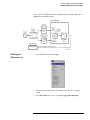
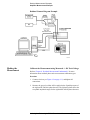
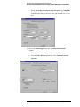
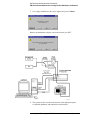
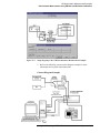
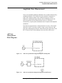
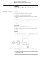
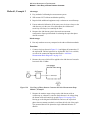
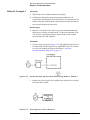
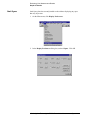
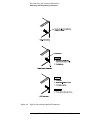
3. When the Connect Diagram dialog box appears, connect the 50 Ω
termination, provided with your system, to the Agilent/HP 70420A test
set’s noise input connector. Refer to “Connect Diagram Example” on
page 3-8 for more information about the correct placement of the 50 Ω
termination.
50 Ω
termination
goes here.
Figure 3-1
Setup Diagram Displayed During the Confidence Test.
Agilent Technologies E5500 Phase Noise Measurement System 3-7
Your First Measurement
Making a Measurement
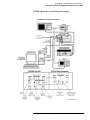
Connect Diagram
Example
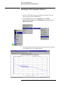
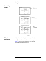
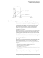
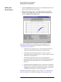
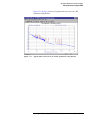
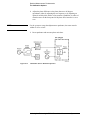
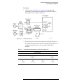
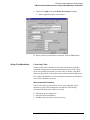
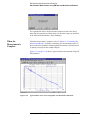
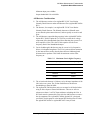
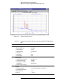
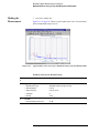
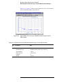
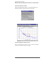
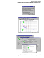
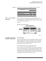
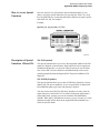
Making the
Measurement
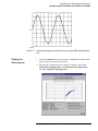
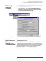
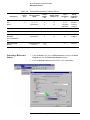
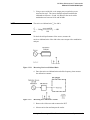
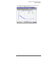
1. Press the Continue key. Because you selected New Measurement to
begin this measurement, the system starts by running the routines
required to calibrate the current measurement setup.
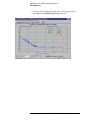
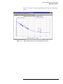
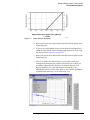
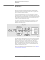
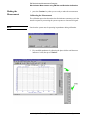
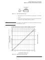
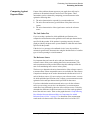
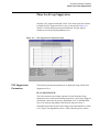
Figure 3-2 shows a typical baseband phase noise plot for an
Agilent/HP 70420A phase noise test set.
3-8 Agilent Technologies E5500 Phase Noise Measurement System
Your First Measurement
Making a Measurement
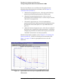
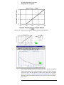
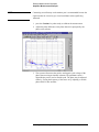
Figure 3-2
Sweep-Segments
Typical Phase Noise Curve for an Agilent/HP 70420A Confidence Test
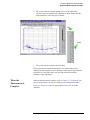
When the system begins measuring noise, it places the noise graph on its
display. As you watch the graph, you will see the system plot its
measurement results in frequency segments.
The system measures the noise level across its frequency offset range by
averaging the noise within smaller frequency segments. This technique
enables the system to optimize measurement speed while providing you with
the measurement resolution needed for most test applications.
Congratulations
You have completed a phase noise measurement. You will find that this
measurement of the Agilent/HP 70420A test set’s internal noise source
provides a convenient way to verify that the system hardware and software
are properly configured for making noise measurements. If your graph looks
like that in Figure 3-2, you now have confidence that your system is
operating normally.
To Learn More
Now continue with this demonstration by turning to Chapter 5, “Expanding
Your Measurement Experience” to learn more about performing phase noise
measurements.
Agilent Technologies E5500 Phase Noise Measurement System 3-9
Your First Measurement
Making a Measurement
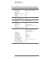
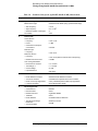
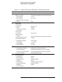
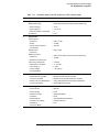
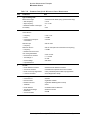
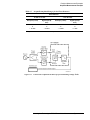
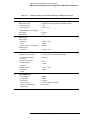
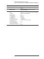
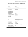
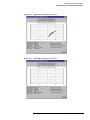
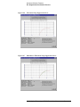
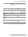
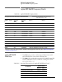
Table 3-1
Parameter Data for the Agilent/HP 70420A Confidence Test Example
Step
Parameters
1
Type and Range Tab
2
Measurement Type
• Baseband Noise (using a test set)
• Start Frequency
• 10 Hz
• Stop Frequency
• 100 E + 6 Hz1
• Minimum Number of Averages
• 4
FFT Quality
• Fast
Swept Quality
• Fast
Cal Tab
• Gain preceding noise input
3
5
• 0 dB
Block Diagram Tab
• Noise Source
4
Data
• Test Set Noise Input
Test Set Tab
Input Attenuation
• 0 dB
LNA Low Pass Filter
• 20 MHz (Auto checked)
• LNA Gain
• Auto Gain (Minimum Auto Gain - 14 dB)
• DC Block
• Not checked
• PLL Integrator Attenuation
• 0 dBm
Graph Tab
• Title
• Confidence Test, Agilent/HP 70420A
Internal Noise Source.
• Graph Type
• Base band noise (dBv/Hz)
• X Scale Minimum
• 10 Hz
• X Scale Maximum
• 100 E + 6 Hz
• Y Scale Minimum
• 0 dBv/Hz
• Y Scale Maximum
• - 200 dBv/Hz
• Normalize trace data to a:
• 1 Hz bandwidth
• Scale trace data to a new
carrier frequency of:
• 1 times the current carrier frequency
• Shift trace data DOWN by:
• 0 dB
• Trace Smoothing Amount
• 0
• Power present at input of DUT
• 0 dB
1. The Stop Frequency depends on the analyzers configured in your phase noise system.
3-10 Agilent Technologies E5500 Phase Noise Measurement System
4
Phase Noise Basics
What You’ll Find in This Chapter
•
What is Phase Noise?, page 4-2
Agilent Technologies E5500 Phase Noise Measurement System 4-1
Phase Noise Basics
What is Phase Noise?
What is Phase Noise?
Frequency stability can be defined as the degree to which an oscillating
source produces the same frequency throughout a specified period of time.
Every RF and microwave source exhibits some amount of frequency
instability. This stability can be broken down into two components:
•
•
long-term stability
short-term stability.
Long term stability describes the frequency variations that occur over long
time periods, expressed in parts per million per hour, day, month, or year.
Short term stability contains all elements causing frequency changes about
the nominal frequency of less than a few seconds duration. The chapter deals
with short-term stability.
Mathematically, an ideal sinewave can be described by
V ( t ) = V o sin 2 π f o t
Where V o = nominal amplitude,
V o sin 2 π f o t = linearly growing phase component,
and f o = nominal frequency
But an actual signal is better modeled by
V ( t ) = Vo + ε ( t ) sin 2 π f o t + ∆φ ( t )
Where ε ( t ) = amplitude fluctuations,
and ∆φ ( t ) = randomly fluctuating phase term or phase noise.
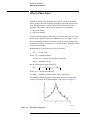
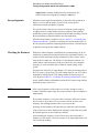
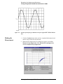
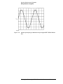
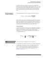
This randomly fluctuating phase term could be observed on an ideal RF
analyzer (one which has no sideband noise of its own) as in Figure 4-1.
Figure 4-1
RF Sideband Spectrum
4-2 Agilent Technologies E5500 Phase Noise Measurement System
Phase Noise Basics
What is Phase Noise?
There are two types of fluctuating phase terms. The first, deterministic, are
discrete signals appearing as distinct components in the spectral density plot.
These signals, commonly called spurious, can be related to known
phenomena in the signal source such as power line frequency, vibration
frequencies, or mixer products.
The second type of phase instability is random in nature, and is commonly
called phase noise. The sources of random sideband noise in an oscillator
include thermal noise, shot noise, and flicker noise.
Many terms exist to quantify the characteristic randomness of phase noise.
Essentially, all methods measure the frequency or phase deviation of the
source under test in the frequency or time domain. Since frequency and
phase are related to each other, all of these terms are also related.
One fundamental description of phase instability or phase noise is spectral
density of phase fluctuations on a per-Hertz basis. The term spectral density
describes the energy distribution as a continuous function, expressed in units
of variance per unit bandwidth. Thus S φ ( f ) (Figure 4-2 on page 4-3) may
be considered as:
2
∆φ 2 rms ( f )
- = rad
-----------S φ ( f ) = -----------------------------------------------------------------------BW used to measure ∆φ rms
Hz
Where BW (bandwidth is negligible with respect to any changes in S φ
versus the fourier frequency or offset frequency (f).
Another useful measure of noise energy is L(f), which is then directly related
to S φ ( f ) by a simple approximation which has generally negligible error if
the modulation sidebands are such that the total phase deviation are much
less than 1 radian (∆φpk<< radian).
1
L ( f ) = --- S ∆φ ( f )
2
Figure 4-2
CW Signal Sidebands viewed in the frequency domain
Agilent Technologies E5500 Phase Noise Measurement System 4-3
Phase Noise Basics
What is Phase Noise?
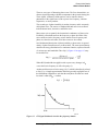
L(f) is an indirect measurement of noise energy easily related to the RF
power spectrum observed on an RF analyzer. Figure 4-3 shows that the
National Institute Science and Technology (NIST) defines L(f) as the ratio
of the power (at an offset (f) Hertz away from the carrier) The phase
modulation sideband is based on a per Hertz of bandwidth spectral density
and or offset frequency in one phase modulation sideband, on a per Hertz of
bandwidth spectral density and (f) equals the Fourier frequency or offset
frequency.
P ssb
power density ( in one phase modulation sideband )
L ( f ) = ---------------------------------------------------------------------------------------------------------------------------------------- = ----------total signal power
Ps
= single sideband (SSB) phase noise to carrier ration (per Hertz)
Figure 4-3
Deriving L(f) from a RF Analyzer Display
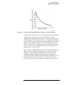
L ( f ) is usually presented logarithmically as a spectral density plot of the
phase modulation sidebands in the frequency domain, expressed in dB
relative to the carrier per Hz (dBc/Hz) as shown in Figure 4-4. This chapter,
except where noted otherwise, will use the logarithmic form of L ( f ) as
follows: S ∆ f ( f ) = 2f 2 L ( f ) .
4-4 Agilent Technologies E5500 Phase Noise Measurement System
Phase Noise Basics
What is Phase Noise?
Figure 4-4
L(f) Described Logarithmically as a Function of Offset Frequency
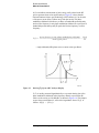
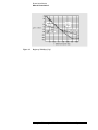
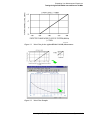
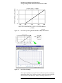
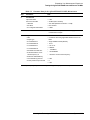
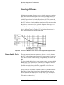
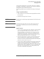
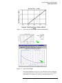
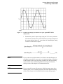
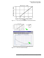
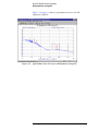
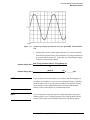
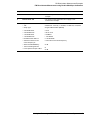
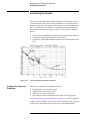
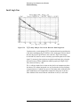
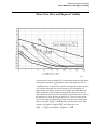
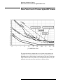
Caution must be exercised when L ( f ) is calculated from the spectral density
of the phase fluctuations S φ ( f ) because the calculation of L ( f ) is
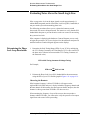
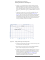
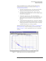
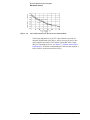
dependent on the small angle criterion. Figure 4-5, the measured phase noise
of a free running VCO described in units of L ( f ) illustrates the erroneous
results that can occur if the instantaneous phase modulation exceeds a small
angle line. Approaching the carrier L ( f ) obviously increases in error as it
indicates a relative level of +45 dBc/Hz at a 1 Hz offset (45 dB more noise
power at a 1 Hz offset in a 1 Hz bandwidth than in the total power of the
signal); which is of course invalid.
Figure 4-5 shows a 10 dB/decade line drawn over the plot, indicating a peak
phase deviation of 0.2 radians integrated over any one decade of offset
frequency. At approximately 0.2 radians the power in the higher order
sidebands of the phase modulation is still insignificant compared to the
power in the first order sideband which insures that the calculation of L ( f )
remains valid. Above the line the plot of L ( f ) becomes increasingly
invalid, and S φ ( f ) must be used to represent the phase noise of the signal.
Agilent Technologies E5500 Phase Noise Measurement System 4-5
Phase Noise Basics
What is Phase Noise?
Figure 4-5
Region of Validity of L(f)
4-6 Agilent Technologies E5500 Phase Noise Measurement System
5
Expanding Your Measurement Experience
What You’ll Find in This Chapter
CAUTION
•
Testing the Agilent/HP 8663A Internal/External 10 MHz, page 5-10
(Conf_8663A_10MHz.pnm)
•
Testing the Agilent/HP 8644B Internal/External 10 MHz, page 5-33
(Conf_8644B_10MHz.pnm)
•
•
•
•
Manual Measurement
Viewing Markers, page 5-56
Omitting Spurs, page 5-57
Displaying the Parameter Summary, page 5-59
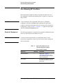
To prevent damage to the Agilent/HP 70420A test set’s hardware
components, the input signal must not be applied to the signal input
connector until the input attenuator has been correctly set for the desired
configuration, as show in Table 5-3 on page 5-17. Apply the input signal
when the connection diagram appears.
Agilent Technologies E5500 Phase Noise Measurement System 5-1
Expanding Your Measurement Experience
Starting the Measurement Software
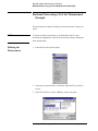
Starting the Measurement Software
1. Make sure your computer and monitor are turned on.
2. Place the Agilent E5500 phase noise measurement software disk in the
disc holder and insert in the CD-ROM drive.
3. Click the Start button, point to Programs, point to Agilent
Measurement Subsystems, point to E5500 Phase Noise, and then click
Measurement Client.
5-2 Agilent Technologies E5500 Phase Noise Measurement System
Expanding Your Measurement Experience
Using the Asset Manager to Add a Source
Using the Asset Manager to Add a Source
The following procedure will configure both the Agilent/HP 70420A phase
noise test set and PC-digitizer so they can be used with the E5500A phase
noise measurement software to make measurements.
NOTE
If you have ordered a preconfigured phase noise system from Agilent
Technologies, skip this step and proceed to “Testing the Agilent/HP 8663A
Internal/External 10 MHz” on page 5-10.
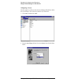
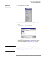
4. Click the System menu, then click Asset Manager.
Agilent Technologies E5500 Phase Noise Measurement System 5-3
Expanding Your Measurement Experience
Using the Asset Manager to Add a Source
Configuring a Source
For this example we will use invoke the Asset Manager Wizard from within
the Asset Manager. This is the most common way to add assets.
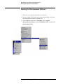
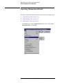
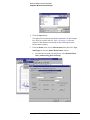
5. Click Asset, and then click Add.
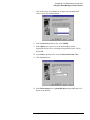
6. From the Asset Type pull-down list, select Source, then click the Next
button.
5-4 Agilent Technologies E5500 Phase Noise Measurement System
Expanding Your Measurement Experience
Using the Asset Manager to Add a Source
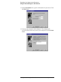
7. Click on the source to be added (for example, the Agilent/HP 8663
sources), then click the Next button.
8. From the Interface pull-down list, select GPIB0.
9. In the Address box, type 19. 19 is the default address for the
Agilent/HP 8663A sources, including the Agilent/HP 8662A, 8663A,
and 8644B.
10. In the Library pull-down list, select the Hewlett-Packard VISA.
11. Click the Next button.
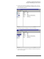
12. In the Model Number box, Agilent/HP 8663A (Agilent/HP-8663 will
appear as the default).
Agilent Technologies E5500 Phase Noise Measurement System 5-5
Expanding Your Measurement Experience
Using the Asset Manager to Add a Source
13. In the Serial Number box, type the serial number for your source. Click
the Next button.
14. You may type a comment in this dialog box. The comment will
associate itself with the asset you have just configured. Click the Finish
button.
5-6 Agilent Technologies E5500 Phase Noise Measurement System
Expanding Your Measurement Experience
Using the Asset Manager to Add a Source
15. You have just used the Asset Manager to configure a source. You will
use the same process to add other software controlled assets to the phase
noise measurement software.
16. click Server, and then click Exit to exit the Asset Manager.
17. Next proceed to “Using the Server Hardware Connections to Specify an
Asset” on the next page.
Agilent Technologies E5500 Phase Noise Measurement System 5-7
Expanding Your Measurement Experience
Using the Server Hardware Connections to Specify the Source
Using the Server Hardware Connections to
Specify the Source
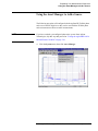
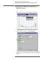
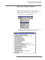
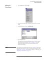
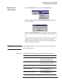
1. From the System menu, choose Server Hardware Connections.
2. From the Test Set pull-down list, select Agilent/HP 8663.
3. A green check-mark will appear after the I/O check has been performed
by the software. If a green check-mark does not appear, click the Check
I/O button.
5-8 Agilent Technologies E5500 Phase Noise Measurement System
Expanding Your Measurement Experience
Using the Server Hardware Connections to Specify the Source
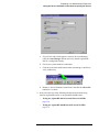
a. If a red circle with a slash appears, return to the Asset Manager
(click the Asset Manager button) and verify that the Agilent/HP
8663A is configured correctly.
b. Check your system hardware connections.
c. Click the green check-mark button on the asset manager’s tool bar to
verify connectivity.
d. Return to “Server Hardware Connections” and click the Check I/O
button for a re-check.
4. Next proceed to one of the following absolute measurements using
either an Agilent/HP 8663A or an Agilent/HP 8644B source:
❍
Testing the Agilent/HP 8663A Internal/External 10 MHz,
page 5-10
❍
Testing the Agilent/HP 8644B Internal/External 10 MHz,
page 5-33
Agilent Technologies E5500 Phase Noise Measurement System 5-9
Expanding Your Measurement Experience
Testing the Agilent/HP 8663A Internal/External 10 MHz
Testing the Agilent/HP 8663A Internal/External
10 MHz
This measurement example will help you measure the absolute phase noise
of an RF synthesizer.
CAUTION
To prevent damage to the Agilent/HP 70420A test set’s hardware
components, the input signal must not be applied to the signal input
connector until the input attenuator has been correctly set for the desired
configuration, as show in Table 5-3 on page 5-17. Apply the input signal
when the Connection Diagram appears.
The following equipment is required for this example in addition to the
phase noise test system and your unit-under-test (UUT).
NOTE
To ensure accurate measurements, you should allow the UUT and
measurement equipment to warm up at least one hour before making the
noise measurement.
Table 5-1
Required Equipment for the
Agilent/HP 8663A 10 MHz
Measurement
Equipment
Quantity
Comments
Agilent/HP 8663A
1
Refer to the “Selecting a
Reference” section of this chapter
for more information about
reference source requirements
Coax Cables
And adequate adapters to connect
the UUT and reference source to
the test set.
5-10 Agilent Technologies E5500 Phase Noise Measurement System
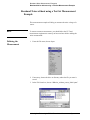
Expanding Your Measurement Experience
Testing the Agilent/HP 8663A Internal/External 10 MHz
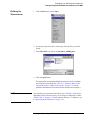
Defining the
Measurement
1. From the File menu, choose Open.
2. If necessary, choose the drive or directory where the file you want is
stored.
3. In the File Name box, choose “Conf_8663A_10MHz.pnm”.
4. Click the Open button.
The appropriate measurement definition parameters for this example
have been pre-stored in this file. Table 5-4, “Parameter Data for the
Agilent/HP 8663A 10 MHz Measurement,” on page 5-31 lists the
parameter data that has been entered for this measurement example.)
NOTE
Note that the source parameters entered for step 2 in Table 5-4 may not be
appropriate for the reference source you are using. To change these values,
refer to Table 5-2 on page 5-12, then continue with step “a”. Otherwise, go
to “Beginning the Measurement” on page 5-16:
Agilent Technologies E5500 Phase Noise Measurement System 5-11
Expanding Your Measurement Experience
Testing the Agilent/HP 8663A Internal/External 10 MHz
a. From the Define menu, choose Measurement; then choose the
Sources tab from the Define Measurement window.
b. Enter the carrier (center) frequency of your UUT (5 MHz to 1.6
GHz). Enter the same frequency for the detector input frequency.
c. Enter the VCO (Nominal) Tuning Constant (see Table 5-2).
d. Enter the Tune Range of VCO (see Table 5-2).
e. Enter the Center Voltage of VCO (see Table 5-2).
f.
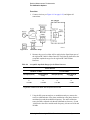
Table 5-2
VCO Source
Agilent/HP 8662/3A
EFC
DCFM
Agilent/HP 8642A/B
Enter the Input Resistance of VCO (see Table 5-2).
Tuning Characteristics for Various Sources
Input
Resistance
(Ω)
Tuning
Calibration
Method
10
10
1E + 6
1 K (8662)
600 (8663)
Measure
Compute
Compute
10
600
Compute
Carrier
Freq.
Tuning Constant
(Hz/V)
Center
Voltage
(V)
Voltage Tuning
Range (± V)
υ0
5 E – 9 x υ0
FM Deviation
0
0
FM Deviation
0
5-12 Agilent Technologies E5500 Phase Noise Measurement System
Expanding Your Measurement Experience
Testing the Agilent/HP 8663A Internal/External 10 MHz
VCO Source
Carrier
Freq.
Agilent/HP 8644B
Other Signal
Generator
DCFM Calibrated for
±1V
Other User VCO
Source
Selecting a Reference
Source
Tuning Constant
(Hz/V)
Center
Voltage
(V)
Voltage Tuning
Range (± V)
Input
Resistance
(Ω)
Tuning
Calibration
Method
FM Deviation
0
10
600
Compute
FM Deviation
0
10
Rin
Compute
Estimated within a
factor of 2
–10 to
+10
1E+6
Measure
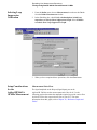
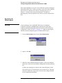
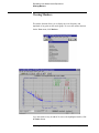
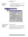
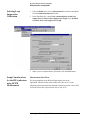
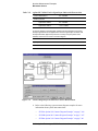
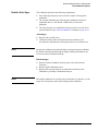
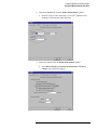
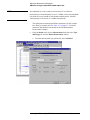
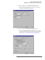
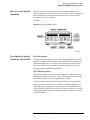
1. From the Define menu, choose Measurement; then choose the Block
Diagram tab from the Define Measurement window.
2. From the Reference Source pull-down list, select HP-8663.
3. When you have completed these operations, click the Close button.
Agilent Technologies E5500 Phase Noise Measurement System 5-13
Expanding Your Measurement Experience
Testing the Agilent/HP 8663A Internal/External 10 MHz
Selecting Loop
Suppression
Verification
1. From the Define menu, choose Measurement; then choose the Cal tab
from the Define Measurement window.
2. In the Cal dialog box, check Verify calculated phase locked loop
supression and Always Show Suppression Graph. Select If limit is
exceeded: Show Loop Suppression Graph.
3. When you have completed these operations, click the Close button.
Setup Considerations
for the
Agilent/HP 8663A
10 MHz Measurement
Measurement Noise Floor
The signal amplitude at the R input (Signal Input) port on the
Agilent/HP 70420A sets the measurement noise floor level. Use the
following graph to determine the amplitude required to provide a noise floor
level that is below the expected noise floor of your UUT. For more
information about this graph, refer to Chapter 18, “Reference Graphs and
Tables”.
5-14 Agilent Technologies E5500 Phase Noise Measurement System
Expanding Your Measurement Experience
Testing the Agilent/HP 8663A Internal/External 10 MHz
Figure 5-1
Noise Floor for the Agilent/HP 8663 10 MHz Measurement
Figure 5-2
Noise Floor Example
Agilent Technologies E5500 Phase Noise Measurement System 5-15
Expanding Your Measurement Experience
Testing the Agilent/HP 8663A Internal/External 10 MHz
If the output amplitude of your UUT is not sufficient to provide an adequate
measurement noise floor, it will be necessary to insert a low-noise amplifier
between the UUT and the test set. Refer to “Inserting an Device” in
Chapter 6, “Absolute Measurement Fundamentals” for details on
determining the effect the amplifiers noise will have on the measured noise
floor.
Beginning the
Measurement
CAUTION
To prevent damage to the Agilent/HP 70420A test set’s hardware
components, the input signal must not be applied to the signal input
connector until the input attenuator has been correctly set for the desired
configuration, as show in Table 5-3 on page 5-17. Apply the input signals
when the connection diagram appears, as shown below in step 3.
1. From the Measurement menu, choose New Measurement.
2. appears, click OK.
3. When the Connect Diagram dialog box appears, click on the hardware
down arrow and select your hardware configuration from the pull-down
list.
Confirm your connections as shown in the Connect Diagram. At this
time connect your UUT and reference sources to the test set. The input
attenuator (Option 001 only) has now been correctly configured based
on your measurement definition.
5-16 Agilent Technologies E5500 Phase Noise Measurement System
Expanding Your Measurement Experience
Testing the Agilent/HP 8663A Internal/External 10 MHz
CAUTION
The Agilent/HP 70420A test set’s signal input is subject to the following
limits and characteristics:
Table 5-3
Agilent/HP 70420A Test Set Signal Input Limits and Characteristics
Limits
Frequency
50 kHz to 26.5 GHz
Maximum Signal Input Power
+30 dBm
At Attenuator Output, Operating Level
Range:
• RF Phase Detectors
0 to +23 dBm
• Microwave Phase Detectors
0 to +5 dBm
• Internal AM Detector
0 to +20 dBm
• Downconverters:
Agilent/HP 70422A
0 to +30 dBm
Agilent/HP 70427A
+5 to +15 dBm
CAUTION:
To prevent damage to the Agilent/HP 70420A Test Set’s hardware components,
the input signal must not be applied to the test set’s signal input connector until
the input attenuator (Option 001) has been set by the phase noise software,
which will occur at the connection diagram.
Characteristics:
Input Impedance
50 ohm Nominal
AM Noise
dc coupled to 50 ohm load
Agilent Technologies E5500 Phase Noise Measurement System 5-17
Expanding Your Measurement Experience
Testing the Agilent/HP 8663A Internal/External 10 MHz
Figure 5-3
Connect Diagram for the Agilent/HP 8663A 10 MHz Measurement
4. Refer to the following system connect diagram examples for more
information about system interconnections :
NOTE
❍
“E5501A Standard Connect Diagram Example” on page 5-19
❍
“E5501B Standard Connect Diagram Example” on page 5-20
❍
“E5502A Opt. 001 Connect Diagram Example” on page 5-21
❍
“E5502A Opt. 001 Connect Diagram Example” on page 5-21
❍
“E5503A Option 001 Connect Diagram Example” on page 5-23
❍
“E5503B Option 001 Connect Diagram Example” on page 5-24
❍
“E5504A Option 201 Connect Diagram Example” on page 5-25
❍
“E5504A Option 201 Connect Diagram Example” on page 5-25
For additional examples, refer to Chapter 19, “Connect Diagrams”
5-18 Agilent Technologies E5500 Phase Noise Measurement System
Expanding Your Measurement Experience
Testing the Agilent/HP 8663A Internal/External 10 MHz
E5501A Standard Connect Diagram Example
Agilent Technologies E5500 Phase Noise Measurement System 5-19
Expanding Your Measurement Experience
Testing the Agilent/HP 8663A Internal/External 10 MHz
E5501B Standard Connect Diagram Example
5-20 Agilent Technologies E5500 Phase Noise Measurement System
Expanding Your Measurement Experience
Testing the Agilent/HP 8663A Internal/External 10 MHz
E5502A Opt. 001 Connect Diagram Example
Agilent Technologies E5500 Phase Noise Measurement System 5-21
Expanding Your Measurement Experience
Testing the Agilent/HP 8663A Internal/External 10 MHz
E5502B Opt. 001 Connect Diagram Example
5-22 Agilent Technologies E5500 Phase Noise Measurement System
Expanding Your Measurement Experience
Testing the Agilent/HP 8663A Internal/External 10 MHz
E5503A Option 001 Connect Diagram Example
Agilent Technologies E5500 Phase Noise Measurement System 5-23
Expanding Your Measurement Experience
Testing the Agilent/HP 8663A Internal/External 10 MHz
E5503B Option 001 Connect Diagram Example
5-24 Agilent Technologies E5500 Phase Noise Measurement System
Expanding Your Measurement Experience
Testing the Agilent/HP 8663A Internal/External 10 MHz
E5504A Option 201 Connect Diagram Example
Agilent Technologies E5500 Phase Noise Measurement System 5-25
Expanding Your Measurement Experience
Testing the Agilent/HP 8663A Internal/External 10 MHz
E5504B Option 201 Connect Diagram Example
5-26 Agilent Technologies E5500 Phase Noise Measurement System
Expanding Your Measurement Experience
Testing the Agilent/HP 8663A Internal/External 10 MHz
5. The following messages will appear on the display as the system
performs the calibration routines. (You will have time to read through
these message descriptions while the system completes the routines.)
Determining Presence of Beat Note...
An initial check is made to verify that a beatnote is present within the
system’s detection range.
Verifying zero-beat...
The frequency of the beatnote is measured to see if it is within 5% of the
estimated Peak Tuning Range of the system. The system’s Peak Tuning
Range is the portion of the voltage-controlled-oscillator (VCO) source’s
tuning range being used for the measurement.
When the system measures the phase noise of a signal source using the
Phase Lock Loop technique (the technique being used in this example) it
requires that one of the two sources used in the setup is a VCO. As you will
see later in this demonstration, you will be required to estimate the tuning
range of the VCO source you are using when you set up your own Phase
Lock Loop measurements.
Zero beating sources...
The center frequencies of the sources are now adjusted, if necessary, to
position the beatnote within the 5% range. The adjustment is made with the
tune voltage applied to the VCO source set at its nominal or center position.
Measuring the VCO Tuning Constant...
The tuning sensitivity (Hz/V) of the VCO source is now precisely
determined by measuring the beatnote frequency at four tune voltage
settings across the tuning range of the VCO source. Linearity across the
tuning range is also verified
Measuring the Phase Detector Constant...
The transfer characteristics (V/rad) of the test set’s phase detector are now
determined for the specific center frequency and power level of the sources
being measured.
Measuring PLL suppression...
The required correction data is created to compensate for the phase noise
suppression which occurs within the bandwidth of the phase lock loop
created for this measurement.
6. The computer displays the PLL suppression curve and associated
measurement values. Press Continue using Adjusted Loop
Agilent Technologies E5500 Phase Noise Measurement System 5-27
Expanding Your Measurement Experience
Testing the Agilent/HP 8663A Internal/External 10 MHz
Suppression to continue making the noise measurement. The
measurement can be stopped by pressing the Abort key.
Sweep-Segments
When the system begins measuring noise, it places the noise graph on its
display. As you watch the graph, you will see the system plot its
measurement results in frequency segments.
The system measures the noise level across its frequency offset range by
averaging the noise within smaller frequency segments. This technique
enables the system to optimize measurement speed while providing you with
the measurement resolution needed for most test applications.
When the measurement is complete, refer to Chapter 15, “Evaluating Your
Measurement Results” for help in evaluating your measurement results. (If
the test system has problems completing the measurement, it will inform you
by placing a message on the computer display.
Checking the Beatnote
While the Connect Diagram is still displayed, recommend that you use an
oscilloscope (connected to the Monitor port on the Agilent/HP 70420A) or a
counter to check the beatnote being created between the reference source
and your device-under-test. The objective of checking the beatnote is to
ensure that the center frequencies of the two sources are close enough in
frequency to create a beatnote that is within the Capture Range of the
system.
The phase lock loop (PLL) Capture Range is 5% of the peak tuning range of
the VCO source you are using. (The peak tuning range for your VCO can be
estimated by multiplying the VCO tuning constant by the tune range of
VCO. Refer to Chapter 15, “Evaluating Your Measurement Results” if you
are not familiar with the relationship between the PLL capture range and the
peak tuning range of the VCO.)
NOTE
If the center frequencies of the sources are not close enough to create a
beatnote within the capture range, the system will not be able to complete its
measurement.
The beatnote frequency is set by the relative frequency difference between
the two sources. If you have two very accurate sources set at the same
frequency, the resulting beatnote will be very close to 0 Hz.
Searching for the beatnote will require that you adjust the center frequency
of one of the sources above and below the frequency of the other source until
the beatnote appears on the oscilloscope’s display.
If incrementing the frequency of one of the sources does not produce a
beatnote, you will need to verify the presence of an output signal from each
source before proceeding.
5-28 Agilent Technologies E5500 Phase Noise Measurement System
Expanding Your Measurement Experience
Testing the Agilent/HP 8663A Internal/External 10 MHz
Figure 5-4
Making the
Measurement
Oscilloscope Display of a Beatnote out of the Agilent/HP 70420A Monitor
Port
1. Click the Continue button when you have completed the beatnote check
and are ready to make the measurement.
2. When the PLL Suppression Curve dialog box appears, select View
Measured Loop Suppression, View Smoothed Loop Suppression,
and View Adjusted Loop Suppression.
Agilent Technologies E5500 Phase Noise Measurement System 5-29
Expanding Your Measurement Experience
Testing the Agilent/HP 8663A Internal/External 10 MHz
There are four different curves available for the this graph (for more
information about loop suppression verification, refer to Chapter 16,
“Advanced Software Features”):
a. “Measured” loop suppression curve - this is the result of the loop
suppression measurement performed by the E5500 system;
b. “Smoothed” measured suppression curve - this is a curve-fit
representation of the measured results, it is used to compare with the
“theoretical” loop suppression;
c. “Theoretical” suppression curve - this is the predicted loop
suppression based on the initial loop parameters defined/selected for
this particular measurement (kphi, kvco, loop bandwidth, filters,
gain, etc).
d. “Adjusted” theoretical suppression curve - this is the new “adjusted”
theoretical value of suppression for this measurement - it is based on
changing loop parameters (in the theoretical response) to match the
“smoothed” measured curve as closely as possible;
When the measurement is complete, refer to Chapter 15, “Evaluating Your
Measurement Results” for help in evaluating your measurement results.
Figure 5-5 on page 5-30 shows a typical phase noise curve for a RF
Synthesizer.
Figure 5-5
Typical Phase Noise Curve for an Agilent/HP 8663A 10 MHz
Measurement.
5-30 Agilent Technologies E5500 Phase Noise Measurement System
Expanding Your Measurement Experience
Testing the Agilent/HP 8663A Internal/External 10 MHz
Table 5-4
Parameter Data for the Agilent/HP 8663A 10 MHz Measurement
Step
Parameters
1
Type and Range Tab
2
Data
Measurement Type
• Absolute Phase Noise (using a phase locked loop)
• Start Frequency
• 10 Hz
• Stop Frequency
• 2 E + 6 Hz1
• Minimum Number of Averages
• 4
FFT Quality
• Fast
Sources Tab
Carrier Source
• Frequency
• 10 E + 6 Hz
• Power
• 7 dBm
• Carrier Source Output is
connected to:
• Test Set
Detector Input
• 10 E +6 Hz
• Frequency
Reference Source
• 10 E +6 Hz (same as Carrier Source Frequency)
• Frequency
• 16 dBm
• Reference Source Power
VCO Tuning Parameters
• 1 E +3 Hz/V
• Nominal Tune Constant
• +/- 10 Volts
• Tune Range +/-
• 0 Volts
• Center Voltage
• 600 ohms
• Input Resistance
3
4
Cal Tab
• Phase Detector Constant
• Measure Phase Detector Constant
• VCO Tune Constant
• Calculate from expected VCO Tune Constant
• Phase Lock Loop Suppression
• Verify calculated phase locked loop suppression
• If Limit is exceeded
• Show Suppression Graph
Block Diagram Tab
• Carrier Source
• Manual
• Downconverter
• None
• Reference Source
• Agilent/HP 8663A
• Timebase
• None
• Phase Detector
• Automatic Detector Selection
• Test Set Tune Voltage
Destination
• Reference Source
• DCFM
• VCO Tune Mode
Agilent Technologies E5500 Phase Noise Measurement System 5-31
Expanding Your Measurement Experience
Testing the Agilent/HP 8663A Internal/External 10 MHz
Table 5-4
Parameter Data for the Agilent/HP 8663A 10 MHz Measurement
Step
Parameters
Data
5
Test Set Tab
Input Attenuation
• 0 dB
LNA Low Pass Filter
• 20 MHz (Auto checked)
• LNA Gain
• Auto Gain (Minimum Auto Gain - 14 dB)
• DC Block
• Not checked
• PLL Integrator Attenuation
• 0 dBm
6
Dowconverter Tab
• The downconverter parameters do not apply to this
measurement example.
7
Graph Tab
• Title
• Graph Type
• Confidence Test using Agilent/HP 8663A Int vs Ext 10
MHz
• X Scale Minimum
• Single-sideband Noise (dBc/Hz)
• X Scale Maximum
• 10 Hz
• Y Scale Minimum
• 4 E + 6 Hz
• Y Scale Maximum
• 0 dBc/Hz
• Normalize trace data to a:
• - 170 dBc/Hz
• Scale trace data to a new
carrier frequency of:
• 1 Hz bandwidth
• 1 times the current carrier frequency
• Shift trace data DOWN by:
• Trace Smoothing Amount
• 0 dB
• Power present at input of DUT
• 0
• 0 dB
1. The Stop Frequency depends on the analyzers configured in your phase noise system.
5-32 Agilent Technologies E5500 Phase Noise Measurement System
Expanding Your Measurement Experience
Testing the Agilent/HP 8644B Internal/External 10 MHz
Testing the Agilent/HP 8644B Internal/External
10 MHz
This measurement example will help you measure the absolute phase noise
of an RF synthesizer.
CAUTION
To prevent damage to the Agilent/HP 70420A test set’s hardware
components, the input signal must not be applied to the signal input
connector until the input attenuator has been correctly set for the desired
configuration, as show in Table 5-7 on page 5-40. Apply the input signal
when the Connection Diagram appears.
The following equipment is required for this example in addition to the
phase noise test system and your unit-under-test (UUT).
NOTE
To ensure accurate measurements, you should allow the UUT and
measurement equipment to warm up at least one hour before making the
noise measurement.
Table 5-5
Required Equipment for the
Agilent/HP 8644B 10 MHz
Measurement
Equipment
Quantity
Comments
Agilent/HP 8663A
1
Refer to the “Selecting a
Reference” section of this chapter
for more information about
reference source requirements
Coax Cables
And adequate adapters to connect
the UUT and reference source to
the test set.
Agilent Technologies E5500 Phase Noise Measurement System 5-33
Expanding Your Measurement Experience
Testing the Agilent/HP 8644B Internal/External 10 MHz
Defining the
Measurement
1. From the File menu, choose Open.
2. If necessary, choose the drive or directory where the file you want is
stored.
3. In the File Name box, choose “Conf_8644B_10MHz.pnm”.
4. Click the Open button.
The appropriate measurement definition parameters for this example
have been pre-stored in this file. Table 5-8 on page 5-54 lists the
parameter data that has been entered for the RF Synthesizer using
DCFM measurement example.)
NOTE
Note that the source parameters entered for step 2 in Table 5-8 may not be
appropriate for the reference source you are using. To change these values,
refer to Table 5-8 on page 5-54, then continue with step “a”. Otherwise, go
to “Beginning the Measurement” on page 5-39:
5-34 Agilent Technologies E5500 Phase Noise Measurement System
Expanding Your Measurement Experience
Testing the Agilent/HP 8644B Internal/External 10 MHz
a. From the Define menu, choose Measurement; then choose the
Sources tab from the Define Measurement window.
b. Enter the carrier (center) frequency of your UUT (5 MHz to 1.6
GHz). Enter the same frequency for the detector input frequency.
c. Enter the VCO (Nominal) Tuning Constant (see Table 5-6).
d. Enter the Tune Range of VCO (see Table 5-6).
e. Enter the Center Voltage of VCO (see Table 5-6).
f.
Table 5-6
VCO Source
Agilent/HP 8662/3A
EFC
DCFM
Agilent/HP 8642A/B
Enter the Input Resistance of VCO (see Table 5-6).
Tuning Characteristics for Various Sources
Input
Resistance
(Ω)
Tuning
Calibration
Method
10
10
1E + 6
1 K (8662)
600 (8663)
Measure
Compute
Compute
10
600
Compute
Carrier
Freq.
Tuning Constant
(Hz/V)
Center
Voltage
(V)
Voltage Tuning
Range (± V)
υ0
5 E – 9 x υ0
FM Deviation
0
0
FM Deviation
0
Agilent Technologies E5500 Phase Noise Measurement System 5-35
Expanding Your Measurement Experience
Testing the Agilent/HP 8644B Internal/External 10 MHz
VCO Source
Carrier
Freq.
Agilent/HP 8644B
Other Signal
Generator
DCFM Calibrated for
±1V
Other User VCO
Source
Selecting a Reference
Source
Tuning Constant
(Hz/V)
Center
Voltage
(V)
Voltage Tuning
Range (± V)
Input
Resistance
(Ω)
Tuning
Calibration
Method
FM Deviation
0
10
600
Compute
FM Deviation
0
10
Rin
Compute
Estimated within a
factor of 2
–10 to
+10
1E+6
Measure
1. From the Define menu, choose Measurement; then choose the Block
Diagram tab from the Define Measurement window.
2. From the Reference Source pull-down list, select HP-8644.
3. When you have completed these operations, click the Close button.
5-36 Agilent Technologies E5500 Phase Noise Measurement System
Expanding Your Measurement Experience
Testing the Agilent/HP 8644B Internal/External 10 MHz
Selecting Loop
Suppression
Verification
1. From the Define menu, choose Measurement; then choose the Cal tab
from the Define Measurement window.
2. In the Cal dialog box, check Verify calculated phase locked loop
supression and Always Show Suppression Graph. Select If limit is
exceeded: Show Loop Suppression Graph.
3. When you have completed these operations, click the Close button.
Setup Considerations
for the
Agilent/HP 8663A
10 MHz Measurement
Measurement Noise Floor
The signal amplitude at the R input (Signal Input) port on the Agilent/HP
70420A sets the measurement noise floor level. Use the following graph to
determine the amplitude required to provide a noise floor level that is below
the expected noise floor of your UUT. For more information about this
graph, refer to Chapter 18, “Reference Graphs and Tables”.
Agilent Technologies E5500 Phase Noise Measurement System 5-37
Expanding Your Measurement Experience
Testing the Agilent/HP 8644B Internal/External 10 MHz
Figure 5-6
Noise Floor for the Agilent/HP 8644B 10 MHz Measurement
Figure 5-7
Noise Floor Example
If the output amplitude of your UUT is not sufficient to provide an adequate
measurement noise floor, it will be necessary to insert a low-noise amplifier
between the UUT and the test set. Refer to “Inserting an Device” in
5-38 Agilent Technologies E5500 Phase Noise Measurement System
Expanding Your Measurement Experience
Testing the Agilent/HP 8644B Internal/External 10 MHz
Chapter 6, “Absolute Measurement Fundamentals” for details on
determining the effect the amplifiers noise will have on the measured noise
floor.
Beginning the
Measurement
CAUTION
To prevent damage to the Agilent/HP 70420A test set’s hardware
components, the input signal must not be applied to the signal input
connector until the input attenuator has been correctly set for the desired
configuration, as show in Table 5-7 on page 5-40. Apply the input signals
when the connection diagram appears, as shown below in step 3.
1. From the Measurement menu, choose New Measurement.
2. appears, click OK.
3. When the Connect Diagram dialog box appears, click on the hardware
down arrow and select your hardware configuration from the pull-down
list.
Confirm your connections as shown in the Connect Diagram. At this
time connect your UUT and reference sources to the test set. The input
attenuator (Option 001 only) has now been correctly configured based
on your measurement definition.
Agilent Technologies E5500 Phase Noise Measurement System 5-39
Expanding Your Measurement Experience
Testing the Agilent/HP 8644B Internal/External 10 MHz
CAUTION
The Agilent/HP 70420A test set’s signal input is subject to the following
limits and characteristics:
Table 5-7
Agilent/HP 70420A Test Set Signal Input Limits and Characteristics
Limits
Frequency
50 kHz to 26.5 GHz
Maximum Signal Input Power
+30 dBm
At Attenuator Output, Operating Level
Range:
• RF Phase Detectors
0 to +23 dBm
• Microwave Phase Detectors
0 to +5 dBm
• Internal AM Detector
0 to +20 dBm
• Downconverters:
Agilent/HP 70422A
0 to +30 dBm
Agilent/HP 70427A
+5 to +15 dBm
CAUTION:
To prevent damage to the Agilent/HP 70420A Test Set’s hardware components,
the input signal must not be applied to the test set’s signal input connector until
the input attenuator (Option 001) has been set by the phase noise software,
which will occur at the connection diagram.
Characteristics:
Input Impedance
50 ohm Nominal
AM Noise
dc coupled to 50 ohm load
5-40 Agilent Technologies E5500 Phase Noise Measurement System
Expanding Your Measurement Experience
Testing the Agilent/HP 8644B Internal/External 10 MHz
Figure 5-8
Connect Diagram for the Agilent/HP 8644B 10 MHz Measurement
4. Refer to the following system connect diagram examples for more
information about system interconnections :
NOTE
❍
“E5501A Standard Connect Diagram Example” on page 5-19
❍
“E5501B Standard Connect Diagram Example” on page 5-20
❍
“E5503A Option 001 Connect Diagram Example” on page 5-23
❍
“E5503B Option 001 Connect Diagram Example” on page 5-47
❍
“E5504A Option 201 Connect Diagram Example” on page 5-48
❍
“E5504B Option 201 Connect Diagram Example” on page 5-49
For additional examples, refer to Chapter 19, “Connect Diagrams”
Agilent Technologies E5500 Phase Noise Measurement System 5-41
Expanding Your Measurement Experience
Testing the Agilent/HP 8644B Internal/External 10 MHz
E5501A Standard Connect Diagram Example
5-42 Agilent Technologies E5500 Phase Noise Measurement System
Expanding Your Measurement Experience
Testing the Agilent/HP 8644B Internal/External 10 MHz
E5501B Standard Connect Diagram Example
Agilent Technologies E5500 Phase Noise Measurement System 5-43
Expanding Your Measurement Experience
Testing the Agilent/HP 8644B Internal/External 10 MHz
E5502A Option 001 Connect Diagram Example
5-44 Agilent Technologies E5500 Phase Noise Measurement System
Expanding Your Measurement Experience
Testing the Agilent/HP 8644B Internal/External 10 MHz
E5502B Option 001 Connect Diagram Example
Agilent Technologies E5500 Phase Noise Measurement System 5-45
Expanding Your Measurement Experience
Testing the Agilent/HP 8644B Internal/External 10 MHz
E5503A Option 001 Connect Diagram Example
5-46 Agilent Technologies E5500 Phase Noise Measurement System
Expanding Your Measurement Experience
Testing the Agilent/HP 8644B Internal/External 10 MHz
E5503B Option 001 Connect Diagram Example
Agilent Technologies E5500 Phase Noise Measurement System 5-47
Expanding Your Measurement Experience
Testing the Agilent/HP 8644B Internal/External 10 MHz
E5504A Option 201 Connect Diagram Example
5-48 Agilent Technologies E5500 Phase Noise Measurement System
Expanding Your Measurement Experience
Testing the Agilent/HP 8644B Internal/External 10 MHz
E5504B Option 201 Connect Diagram Example
Agilent Technologies E5500 Phase Noise Measurement System 5-49
Expanding Your Measurement Experience
Testing the Agilent/HP 8644B Internal/External 10 MHz
5. The following messages will appear on the display as the system
performs the calibration routines. (You will have time to read through
these message descriptions while the system completes the routines.)
Determining Presence of Beat Note...
An initial check is made to verify that a beatnote is present within the
system’s detection range.
Verifying zero-beat...
The frequency of the beatnote is measured to see if it is within 5% of the
estimated Peak Tuning Range of the system. The system’s Peak Tuning
Range is the portion of the voltage-controlled-oscillator (VCO) source’s
tuning range being used for the measurement.
When the system measures the phase noise of a signal source using the
Phase Lock Loop technique (the technique being used in this example) it
requires that one of the two sources used in the setup is a VCO. As you will
see later in this demonstration, you will be required to estimate the tuning
range of the VCO source you are using when you set up your own Phase
Lock Loop measurements.
Zero beating sources...
The center frequencies of the sources are now adjusted, if necessary, to
position the beatnote within the 5% range. The adjustment is made with the
tune voltage applied to the VCO source set at its nominal or center position.
Measuring the VCO Tuning Constant...
The tuning sensitivity (Hz/V) of the VCO source is now precisely
determined by measuring the beatnote frequency at four tune voltage
settings across the tuning range of the VCO source. Linearity across the
tuning range is also verified
Measuring the Phase Detector Constant...
The transfer characteristics (V/rad) of the test set’s phase detector are now
determined for the specific center frequency and power level of the sources
being measured.
Measuring PLL suppression...
The required correction data is created to compensate for the phase noise
suppression which occurs within the bandwidth of the phase lock loop
created for this measurement.
6. The computer displays the PLL suppression curve and associated
measurement values. Press Continue using Adjusted Loop
5-50 Agilent Technologies E5500 Phase Noise Measurement System
Expanding Your Measurement Experience
Testing the Agilent/HP 8644B Internal/External 10 MHz
Suppression to continue making the noise measurement. The
measurement can be stopped by pressing the Abort key.
Sweep-Segments
When the system begins measuring noise, it places the noise graph on its
display. As you watch the graph, you will see the system plot its
measurement results in frequency segments.
The system measures the noise level across its frequency offset range by
averaging the noise within smaller frequency segments. This technique
enables the system to optimize measurement speed while providing you with
the measurement resolution needed for most test applications.
When the measurement is complete, refer to Chapter 15, “Evaluating Your
Measurement Results” for help in evaluating your measurement results. (If
the test system has problems completing the measurement, it will inform you
by placing a message on the computer display.
Checking the Beatnote
While the Connect Diagram is still displayed, recommend that you use an
oscilloscope (connected to the Monitor port on the Agilent/HP 70420A) or a
counter to check the beatnote being created between the reference source
and your device-under-test. The objective of checking the beatnote is to
ensure that the center frequencies of the two sources are close enough in
frequency to create a beatnote that is within the Capture Range of the
system.
The phase lock loop (PLL) Capture Range is 5% of the peak tuning range of
the VCO source you are using. (The peak tuning range for your VCO can be
estimated by multiplying the VCO tuning constant by the tune range of
VCO. Refer to Chapter 15, “Evaluating Your Measurement Results” if you
are not familiar with the relationship between the PLL capture range and the
peak tuning range of the VCO.)
NOTE
If the center frequencies of the sources are not close enough to create a
beatnote within the capture range, the system will not be able to complete its
measurement.
The beatnote frequency is set by the relative frequency difference between
the two sources. If you have two very accurate sources set at the same
frequency, the resulting beatnote will be very close to 0 Hz.
Searching for the beatnote will require that you adjust the center frequency
of one of the sources above and below the frequency of the other source until
the beatnote appears on the oscilloscope’s display.
If incrementing the frequency of one of the sources does not produce a
beatnote, you will need to verify the presence of an output signal from each
source before proceeding.
Agilent Technologies E5500 Phase Noise Measurement System 5-51
Expanding Your Measurement Experience
Testing the Agilent/HP 8644B Internal/External 10 MHz
Figure 5-9
Making the
Measurement
Oscilloscope Display of a Beatnote out of the Agilent/HP 70420A Monitor
Port
1. Click the Continue button when you have completed the beatnote check
and are ready to make the measurement.
2. When the PLL Suppression Curve dialog box appears, select View
Measured Loop Suppression, View Smoothed Loop Suppression,
and View Adjusted Loop Suppression.
5-52 Agilent Technologies E5500 Phase Noise Measurement System
Expanding Your Measurement Experience
Testing the Agilent/HP 8644B Internal/External 10 MHz
There are four different curves available for the this graph (for more
information about loop suppression verification, refer to Chapter 16,
“Advanced Software Features”):
a. “Measured” loop suppression curve - this is the result of the loop
suppression measurement performed by the E5500 system;
b. “Smoothed” measured suppression curve - this is a curve-fit
representation of the measured results, it is used to compare with the
“theoretical” loop suppression;
c. “Theoretical” suppression curve - this is the predicted loop
suppression based on the initial loop parameters defined/selected for
this particular measurement (kphi, kvco, loop bandwidth, filters,
gain, etc).
d. “Adjusted” theoretical suppression curve - this is the new “adjusted”
theoretical value of suppression for this measurement - it is based on
changing loop parameters (in the theoretical response) to match the
“smoothed” measured curve as closely as possible;
When the measurement is complete, refer to Chapter 15, “Evaluating Your
Measurement Results” for help in evaluating your measurement results.
Figure 5-5 on page 5-30 shows a typical phase noise curve for a RF
Synthesizer.
Figure 5-10
Typical Phase Noise Curve for an Agilent/HP 8644B 10 MHz
Measurement.
Agilent Technologies E5500 Phase Noise Measurement System 5-53
Expanding Your Measurement Experience
Testing the Agilent/HP 8644B Internal/External 10 MHz
Table 5-8
Parameter Data for the Agilent/HP 8644B 10 MHz Measurement
Step
Parameters
1
Type and Range Tab
2
Data
Measurement Type
• Absolute Phase Noise (using a phase locked loop)
• Start Frequency
• 10 Hz
• Stop Frequency
• 2 E + 6 Hz1
• Minimum Number of Averages
• 4
FFT Quality
• Fast
Sources Tab
Carrier Source
• Frequency
• 10 E + 6 Hz
• Power
• 7 dBm
• Carrier Source Output is
connected to:
• Test Set
Detector Input
• Frequency
• 10 E +6 Hz
Reference Source
• Frequency
• 10 E +6 Hz (same as Carrier Source Frequency)
• Reference Source Power
• 16 dBm
VCO Tuning Parameters
3
4
• Nominal Tune Constant
• 1 E +3 Hz/V
• Tune Range +/-
• +/- 10 Volts
• Center Voltage
• 0 Volts
• Input Resistance
• 600 ohms
Cal Tab
• Phase Detector Constant
• Measure Phase Detector Constant
• VCO Tune Constant
• Calculate from expected VCO Tune Constant
• Phase Lock Loop Suppression
• Verify calculated phase locked loop suppression
• If Limit is exceeded
• Show Suppression Graph
Block Diagram Tab
• Carrier Source
• Manual
• Downconverter
• None
• Reference Source
• Agilent/HP 8644B
• Timebase
• None
• Phase Detector
• Automatic Detector Selection
• Test Set Tune Voltage
Destination
• Reference Source
• DCFM
• VCO Tune Mode
5-54 Agilent Technologies E5500 Phase Noise Measurement System
Expanding Your Measurement Experience
Testing the Agilent/HP 8644B Internal/External 10 MHz
Table 5-8
Parameter Data for the Agilent/HP 8644B 10 MHz Measurement
Step
Parameters
5
Test Set Tab
Data
Input Attenuation
• 0 dB
LNA Low Pass Filter
• 20 MHz (Auto checked)
• LNA Gain
• Auto Gain (Minimum Auto Gain - 14 dB)
• DC Block
• Not checked
• PLL Integrator Attenuation
• 0 dBm
6
Dowconverter Tab
• The downconverter parameters do not apply to this
measurement example.
7
Graph Tab
• Title
• Graph Type
• Confidence Test using Agilent/HP 8644B Int vs Ext 10
MHz
• X Scale Minimum
• Single-sideband Noise (dBc/Hz)
• X Scale Maximum
• 10 Hz
• Y Scale Minimum
• 4 E + 6 Hz
• Y Scale Maximum
• 0 dBc/Hz
• Normalize trace data to a:
• - 170 dBc/Hz
• Scale trace data to a new
carrier frequency of:
• 1 Hz bandwidth
• 1 times the current carrier frequency
• Shift trace data DOWN by:
• Trace Smoothing Amount
• 0 dB
• Power present at input of DUT
• 0
• 0 dB
1. The Stop Frequency depends on the analyzers configured in your phase noise system.
Agilent Technologies E5500 Phase Noise Measurement System 5-55
Expanding Your Measurement Experience
Viewing Markers
Viewing Markers
The marker function allows you to display the exact frequency and
amplitude of any point on the results graph. To access the marker function:
On the View menu, click Markers.
Up to nine markers may be added. To remove the highlighted marker, click
the Delete button.
5-56 Agilent Technologies E5500 Phase Noise Measurement System
Expanding Your Measurement Experience
Omitting Spurs
Omitting Spurs
The Omit Spurs function plots the currently loaded results without
displaying any spurs that may be present.
1. On the View menu, click Display Preferences.
2. In the Display Preferences dialog box, uncheck Spurs. Click OK
Agilent Technologies E5500 Phase Noise Measurement System 5-57
Expanding Your Measurement Experience
Omitting Spurs
3. The Graph will be displayed without spurs. To re-display the spurs,
check Spurs in the Display Preferences dialog box.
5-58 Agilent Technologies E5500 Phase Noise Measurement System
Expanding Your Measurement Experience
Displaying the Parameter Summary
Displaying the Parameter Summary
The Parameter Summary function allows you to quickly review the
measurement parameter entries that were used for this measurement. The
parameter summary data is included when you print the graph.
1. On the View menu, click Parameter Summay.
2. The Parameter Summary Notepad dialog box appears. The data can
be printed or changed using standard Notepad functionality.
Agilent Technologies E5500 Phase Noise Measurement System 5-59
Expanding Your Measurement Experience
Exporting Measurement Results
Exporting Measurement Results
The Export Measurement Results function exports data in one of three types:
•
•
•
“Exporting Trace Data” on page 5-61
“Exporting Spur Data” on page 5-62
“Exporting X-Y Data” on page 5-63
1. On the File menu, point to Export Results, then click on either Trace
Data, Spur Data, or X-Y Data.
5-60 Agilent Technologies E5500 Phase Noise Measurement System
Expanding Your Measurement Experience
Exporting Measurement Results
Exporting Trace Data
1. On the File menu, point to Export Results, then click on Trace Data.
Agilent Technologies E5500 Phase Noise Measurement System 5-61
Expanding Your Measurement Experience
Exporting Measurement Results
Exporting Spur Data
1. On the File menu, point to Export Results, then click on Spur Data.
5-62 Agilent Technologies E5500 Phase Noise Measurement System
Expanding Your Measurement Experience
Exporting Measurement Results
Exporting X-Y Data
1. On the File menu, point to Export Results, then click on X-Y Data.
Agilent Technologies E5500 Phase Noise Measurement System 5-63
6
Absolute Measurement Fundamentals
What You’ll Find in This Chapter
This chapter contains information about making absolute phase noise
measurements of signal sources. This information is fundamental to using
the Agilent E5500 phase noise measurement system. It is important that you
understand the concepts contained in this chapter in order to use the system
effectively.
The topics covered in this chapter include:
•
•
•
•
•
•
•
•
•
The Phase Lock Loop Technique, page 6-2
What Sets the Measurement Noise Floor?, page 6-6
Selecting a Reference, page 6-8
Estimating the Tuning Constant, page 6-11
Tracking Frequency Drift, page 6-12
Changing the PTR, page 6-14
Minimizing Injection Locking, page 6-16
Inserting a Device, page 6-18
Evaluating Noise Above the Small Angle Line, page 6-20
Agilent Technologies E5500 Phase Noise Measurement System 6-1
Absolute Measurement Fundamentals
The Phase Lock Loop Technique
The Phase Lock Loop Technique
The phase lock loop measurement technique requires two signal sources; the
source-under-test and a reference source. This measurement type requires
that one of the two sources is a voltage-controlled-oscillator (VCO).
You will most likely use the phase lock loop technique since it is the
measurement type most commonly used for measuring signal source
devices. This chapter focuses on this measurement type for signal source
measurements.
6-2 Agilent Technologies E5500 Phase Noise Measurement System
Absolute Measurement Fundamentals
The Phase Lock Loop Technique
Understanding the
Phase-Lock Loop
Technique
This measurement technique requires two signal sources set up in a phase
locked loop (PLL) configuration. One of the sources is the unit-under-test
(UUT). The second source serves as the reference against which the UUT is
measured. (One of the two sources must be a VCO source capable of being
frequency tuned by the System.) Figure 6-1 on page 6-3 shows a simplified
diagram of the PLL configuration used for the measurement.
Figure 6-1 Simplified Block Diagram of the Phase Lock Loop Configuration
The Phase Lock Loop
Circuit
The Capture and Drift Tracking Ranges
Like other PLL circuits, the phase lock loop created for the measurement has
a Capture Range and a drift tracking range. The Capture Range is equal to
5% of the system’s peak tuning range, and the drift tracking range is equal to
24% of the system’s peak tuning range.
The system’s peak tuning range is derived from the tuning characteristics of
the VCO source you are using for the measurement. Figure 6-2 on page 6-4
illustrates the relationship that typically exists between the VCO’s
peak-to-peak tuning range and the tuning range of the system.
The system’s drift tracking range is limited to a small portion of the peak
tuning range to minimize the possibility of measurement accuracy
degradation caused by non-linearity across the VCO’s tuning range.
Peak Tune Range (PTR)
PTR is determined using two parameters:
•
•
VCO tuning sensitivity (Hz/Volt)
Total voltage tuning range (Volts)
PTR = (VCO Tuning Sensitivity) X (Total Voltage Tuning Range)
PTR = (100 Hz/V) X (10 V) = 1000 Hz
Agilent Technologies E5500 Phase Noise Measurement System 6-3
Absolute Measurement Fundamentals
The Phase Lock Loop Technique
Figure 6-2 Typical Relationship of Capture Range and Drift Tracking Range to Tuning Range of
VCO
As an Example:
A Peak Tuning Range of 1000 Hz will provide the following ranges:
Capture Range = 0.05 X 1000 Hz = 50 Hz
Drift Tracking Range = 0.24 X 1000 Hz = 240 Hz
Tuning Requirements
The peak tuning range required for your measurement will depend on the
frequency stability of the two sources you are using. The signals from the
two sources are mixed in the system’s phase detector to create a beatnote. In
order for the loop to acquire lock, the center frequencies of the sources must
be close enough together to create a beatnote that is within the system’s
Capture Range. Once the loop is locked, the frequency of the beatnote must
remain within the drift tracking range for the duration of the measurement.
In Figure 6-3 on page 6-5, the ranges calculated in the previous example are
marked to show their relationship to the beatnote frequency.
6-4 Agilent Technologies E5500 Phase Noise Measurement System
Absolute Measurement Fundamentals
The Phase Lock Loop Technique
Figure 6-3 Relationship of Capture and Drift Tracking Ranges to Beatnote Frequency
If the beatnote does not remain within the drift tracking range during the
measurement, the out of lock detector will be set and the System will stop
the measurement. If this happens, you will need to increase the system’s
drift tracking range by increasing the system’s peak tuning range (if
possible) or by selecting a VCO source with a greater tuning range.
Selecting the VCO Source
Although you must select a VCO source that will provide a sufficient tuning
range to permit the system to track the beatnote, keep in mind that a wide
tuning range typically means a higher noise level on the VCO source signal.
When the VCO source for your measurement is also the reference source,
this trade-off can make reference source selection the most critical aspect of
your measurement setup.
Specifying Your VCO Source
When you set up your PLL measurement, you will need to know four things
about the tuning characteristics of the VCO source you are using. The
System will determine the VCO source’s peak tuning range from these four
parameters.
•
•
•
•
Tuning Constant, estimated tuning sensitivity (Hz/V)
Center Voltage of Tuning Range, (V)
Tune Range of VCO, (±V)
Input Resistance of Tuning Port, (ohms) if the tuning constant is not
to be measured.
The measurement examples in the next chapter that recommend a specific
VCO source will provide you with the tuning parameters for the specified
source.
Agilent Technologies E5500 Phase Noise Measurement System 6-5
Absolute Measurement Fundamentals
What Sets the Measurement Noise Floor?
What Sets the Measurement Noise Floor?
The noise floor for your measurement will be set by two things:
•
•
The System Noise
Floor
The noise floor of the phase detector and low-noise amplifier (LNA)
The noise level of the reference source you are using
The noise floor of the system is directly related to the amplitude of the input
signal at the R input port of the system’s phase detector.
The following table shows the amplitude ranges for the L and R ports.
Phase Detector
1.2 to 26.5 GHz1
50 kHz to 1.6 GHz
Ref Input (L Port)
+ 15 dBm
+
to
23 dBM
Signal Input (R
Port)
0 dBm
to
+ 23 dBM
Ref Input (L Port)
+ 7 dBm
+
to
10 dBM
50 kHz to 26.5 GHz2
Signal Input (R
Port)
AM Noise
0 dBm
to
+ 5 dBM
0 dBm
to
20 dBM
1. Agilent/HP 70420A phase noise test set Options 001 and 201with no attenuation
2. Agilent/HP 70420A phase noise test set Option 001 with no attenuation
If the L port (reference input) signal is within the amplitude range shown in
the preceding table, the signal level at the R (signal ) input port sets the noise
floor for the system.
The following graph shows the relationship between the R (signal) input
level and the system noise floor.
6-6 Agilent Technologies E5500 Phase Noise Measurement System
Absolute Measurement Fundamentals
What Sets the Measurement Noise Floor?
Figure 6-4 Relationship Between the R Input Level and System Noise Floor
The Noise Level of the
Reference Source
Unless it is below the system’s noise floor, the noise level of the source you
are using as the reference source will set the noise floor for the
measurement. When you set up your measurement, you will want to use a
reference source with a noise level that is at or below the level of the source
you are going to measure.
The following graph demonstrates that as the noise level of the reference
source approaches the noise level of the UUT, the level measured by the
System (which is the sum of all noise sources affecting the system) is
increased above the actual noise level of the UUT.
Figure 6-5 Increase in Measured Noise as Reference Source Noise Approaches UUT Noise
Agilent Technologies E5500 Phase Noise Measurement System 6-7
Absolute Measurement Fundamentals
Selecting a Reference
Selecting a Reference
Selecting an appropriate reference source is critical when you are making a
phase noise measurement using the phase lock loop technique. The key to
selecting a reference source is to compare the noise level of the reference
with the expected noise level of the unit-under-test (UUT). In general, the
lower the reference source’s noise level is below the expected noise level of
the UUT the better. (Keep in mind that you only need to be concerned about
the reference source’s noise level within the frequency offset range over
which you plan to measure the UUT.)
As shown by the graph in Figure 6-6, the further the reference source’s noise
level is below the noise level of the UUT, the less the reference source’s
noise will contribute to the measurement results.
Figure 6-6
Using a Similar Device
Increase in Measured Noise As UUT Noise Approaches Reference Noise
The test system performs best when you are able to use a device similar to
the UUT as the reference source for your PLL measurement. Of course one
of the devices must be capable of being voltage tuned by the system to do
this.
To select a similar device for use as the reference source, you must establish
that the noise level of the reference source device is adequate to measure
your UUT. The Three Source Comparison technique enables you to
establish the actual noise levels of three comparable devices when two
devices are available in addition to the UUT.
If only one device is available in addition to the UUT, you can perform the
Phase Noise Using a Phase Locked Loop Measurement using these two
devices and know that the noise level of each of the devices is at least as
good as the measured results. (The measured results will represent the sum
of the noise of both devices.)
6-8 Agilent Technologies E5500 Phase Noise Measurement System
Absolute Measurement Fundamentals
Selecting a Reference
Using a Signal
Generator
When using a signal generator as a reference source, it is important that the
generator’s noise characteristics are adequate for measuring your device.
Tuning Requirements
Often the reference source you select will also serve as the VCO source for
the PLL measurement. (The VCO source can be either the unit-under-test
(UUT) or the reference source.) To configure a PLL measurement, you will
need to know the following tuning information about the VCO source you
are using:
•
•
•
•
Tuning Constant (Hz/V) (within a factor of 2)
Tuning Voltage Range (V)
Center Voltage of Tuning Range (V)
Input Resistance of Tuning Port (ohms)
The primary consideration when evaluating a potential VCO source for your
measurement is whether it will provide the test system with sufficient
capture and drift tracking ranges to maintain lock throughout the
measurement. To make this determination, you must estimate what the drift
range of the sources you are using will be over the measurement period
(thirty minutes maximum). (Details on the relationship between the capture
and drift tracking ranges and the tuning range of the VCO source are
provided in Table 6-1. This information will help you evaluate your VCO
source based on the estimated drift of your sources.)
Table 6-1 lists the tuning parameters for several VCO options.
Table 6-1
Tuning Characteristics of Various VCO Source Options
VCO Source
Carrier
Freq.
Tuning Constant
(Hz/V)
Center
Voltage
(V)
Voltage Tuning
Range (± V)
Agilent/HP 8662/3A
EFC
DCFM
υ0
5 E – 9 x υ0
FM Deviation
0
0
Agilent/HP 8642A/B
FM Deviation
Agilent/HP 8644B
Other Signal
Generator
DCFM Calibrated for
±1V
Other User VCO
Source
Input
Resistance
(Ω)
Tuning
Calibration
Method
10
10
1E + 6
1 k (8662)
600 (8663)
Measure
Calculate
Calculate
0
10
600
Calculate
FM Deviation
0
10
600
Calculate
FM Deviation
0
10
Rin
Calculate
Estimated within a
factor of 2
–10 to
+10
See Figure 6-7 on
page 6-10
1E+6
Measure
Agilent Technologies E5500 Phase Noise Measurement System 6-9
Absolute Measurement Fundamentals
Selecting a Reference
Figure 6-7
Agilent/HP 70420A Voltage Tuning Range Limits Relative to Center
Voltage of the VCO Tuning Curve.
6-10 Agilent Technologies E5500 Phase Noise Measurement System
Absolute Measurement Fundamentals
Estimating the Tuning Constant
Estimating the Tuning Constant
The VCO tuning constant is the tuning sensitivity of the VCO source in
Hz/V. The required accuracy of the entered tuning constant value depends
on the VCO tuning constant calibration method specified for the
measurement. The calibration method is selected in the Calibr Process menu.
The following chart lists the calibration method choices and the tuning
constant accuracy required for each.
Table 6-2
VCO Tuning Constant Calibration Method
VCO Tuning Constant Calibration
Method (selected in calibration
screen)
Required Tuning Constant
Accuracy (entered in parameter
screen)
Use the current tuning constant
(must be accurate from a previous
measurement of the same source).
Within a factor of 2 of actual value.
(Enter 1 E + 6 for Input
Resistance.)
Measure the VCO tuning constant
Within a factor of 2 of actual value.
(Enter 1 E + 6 for Input
Resistance.)
Calculate from expected T. Constant
Exact, within 5% of actual.
(Also requires that entered Input
Resistance value is accurate.)
Agilent Technologies E5500 Phase Noise Measurement System 6-11
Absolute Measurement Fundamentals
Tracking Frequency Drift
Tracking Frequency Drift
The system’s frequency drift tracking capability for the phase lock loop
measurement is directly related to the tuning range of the VCO source being
used. The system’s drift tracking range is approximately 24% of the peak
tuning range (PTR) of the VCO.
PTR= VCO Tuning Constant X Voltage Tuning Range
This is the frequency range within which the beatnote signal created by the
Agilent/HP 70420A phase detector must remain throughout the
measurement period. In addition, the beatnote signal must remain within the
system’s Capture Range (5% of the PTR) during the time it takes the system
to calibrate and lock the phase lock loop.
The stability of the beatnote is a function of the combined frequency
stability of the sources being used for the measurement. If beatnote drift
prevents the beatnote from remaining within the Capture Range long enough
for the system to attain phase lock, the computer will inform you by
displaying a message. If the beatnote drifts beyond the drift tracking range
during the measurement, the computer will stop the measurement and
inform you that the system has lost lock.
Evaluating Beatnote
Drift
The Checking the Beatnote section included in each phase lock loop
measurement example in this chapter provides a procedure for adjusting the
beatnote to within the Capture Range set for the measurement. If you have
not done so already, verify that the beatnote signal can be tuned to within the
Capture Range and that it will remain within the range.
Continue to observe the beatnote and verify that it will not drift beyond the
drift tracking range (24% of the PTR) during the measurement period. The
length of the measurement period is primarily a function of the frequency
offset range specified for the measurement (Start to Stop Frequency).
Action
If beatnote drift exceeds the limits of the Capture or drift tracking ranges set
for your measurement, the system will not be able to complete the
measurement. You have two possible alternatives.
1. Minimize beatnote drift.
•
•
By Allowing sources to warm-up sufficiently.
By Selecting a different reference source with less drift.
2. Increase the capture and drift tracking Ranges.
6-12 Agilent Technologies E5500 Phase Noise Measurement System
Absolute Measurement Fundamentals
Tracking Frequency Drift
•
By Selecting a measurement example in this chapter that specifies a drift
rate compatible with the beatnote drift rate you have observed.
By Increasing the peak tuning range for the measurement. (Further
information about increasing the PTR is provided in Changing the PTR.)
Agilent Technologies E5500 Phase Noise Measurement System 6-13
Absolute Measurement Fundamentals
Changing the PTR
Changing the PTR
The peak tuning range (PTR) for the phase lock loop measurement is set by
the tune range entered for the VCO and the VCO’s tuning constant. (If the
calibration technique is set to measure the VCO tuning constant, the
measured value will be used to determine the system’s PTR.)
PTR= VCO Tuning Constant X Voltage Tuning Range
From the PTR, the phase noise software derives the capture and drift
tracking Ranges for the measurement. These ranges set the frequency
stability requirements for the sources being used.
The PTR also determines the phase lock loop (PLL) bandwidth for the
measurement. An important attribute of the PLL bandwidth is that it
suppresses the close-in noise which would otherwise prevent the system
from locking the loop.
The Tuning
Qualifications
Changing the PTR is accomplished by changing the tune range of VCO
value or the VCO tuning constant value or both. There are several ways this
can be done. However, when considering these or any other options for
changing the PTR, it is important to remember that the VCO source must
always meet the following tuning qualifications.
•
•
The tuning response of the VCO source must always remain monotonic.
The VCO source’s output level must remain constant across its tuning
range.
6-14 Agilent Technologies E5500 Phase Noise Measurement System
Absolute Measurement Fundamentals
Changing the PTR
As long as these qualifications are met, and the software does not indicate
any difficulty in establishing its calibration criteria, an increase in PTR will
not degrade the system’s measurement accuracy.
The following methods may be considered for increasing or decreasing the
PTR.
Voltage-Controlled-Oscillators
1. Select a different VCO source that has the tuning capabilities needed for
the measurement.
2. Increase the tune range of the VCO source.
CAUTION
Be careful not to exceed the input voltage limitations of the Tune Port on the
VCO source.
NOTE
Increasing the tune range of the VCO is only valid as long as the VCO
source is able to continuously meet the previously mentioned tuning
qualifications.
Signal Generators
1. If you are using a signal generator with a calibrated 1 Vpk DC FM Input
(such as the Agilent/HP 8640B, 8642A/B, 8656B, or 8662/3), the
Voltage tuning Range can be increased to 10 V as long as you select
Computed from the expected T. Constant in the Calibration Process
display. These signal generators continue to meet all of the previously
mentioned tuning qualifications across a 10V tuning range.
2. Increase the signal generator’s frequency deviation setting and set the
software to measure the new tuning constant or enter the increased
deviation if it is known. (Note that increasing the deviation setting often
increases the source’s noise level as well.)
3. If you are using a synthesizer with Electronic-Frequency-Control (EFC)
capability such as the Agilent/HP 8662A or Agilent/HP 8663A, it is
possible to increase the tuning range of these sources using a VCO as an
external time base. When a compatible VCO source is connected to the
EXT INPUT on the Agilent/HP 8662/3, the tuning capability of the
VCO source is transferred to the synthesizer.
Agilent Technologies E5500 Phase Noise Measurement System 6-15
Absolute Measurement Fundamentals
Minimizing Injection Locking
Minimizing Injection Locking
Injection locking occurs when a signal feeds back into an oscillator through
its output path. This can cause the oscillator to become locked to the injected
signal rather than to the reference signal for the phase locked loop.
Injection locking is possible whenever the buffering at the output of an
oscillator is not sufficient to prevent a signal from entering. If the injection
locking occurs at an offset frequency that is not well within the PLL
bandwidth set for the measurement, it can cause the system to lose phase
lock.
Adding Isolation
The best way to prevent injection locking is to isolate the output of the
source being injection locked (typically the unit-under-test) by increasing
the buffering at its output. This can be accomplished by inserting a low noise
amplifier and/or an attenuator between the output of the source being
injection locked and the Agilent/HP 70420A. (For information on
determining the effect that the amplifier noise will have on the measurement
noise floor, refer to Inserting a Device in this section.)
Increasing the PLL
Bandwidth
If the injection locking bandwidth is less or equal to the PLL bandwidth, it
may be possible to increase the PLL bandwidth sufficiently to complete the
measurement. The PLL bandwidth is increased by increasing the peak
tuning range (PTR) for the measurement.
NOTE
The PTR for the measurement is set by the tuning characteristics of the VCO
source you are using. Notice in Figure 6-8 on page 6-17 that increasing the
PLL bandwidth can require a substantially larger increase in the PTR. For
information on the limitations of increasing the PTR, refer to Changing the
PTR in this section.
To estimate the PTR needed to prevent injection locking from causing the
system to lose lock:
1. Determine the injection locking bandwidth. Tune the beatnote toward 0
Hz using the procedure described in the Checking the Beatnote section
of each phase lock loop measurement example in this chapter. When the
injection locking occurs, the beatnote will disappear. The injection
locking bandwidth is the frequency of the beatnote just prior to where
the injection locking occurs as the beatnote is tuned toward 0 Hz.
6-16 Agilent Technologies E5500 Phase Noise Measurement System
Absolute Measurement Fundamentals
Minimizing Injection Locking
2. Multiply the injection locking bandwidth by 2 to determine the
minimum PLL bandwidth required to prevent the injection locking from
causing the system to lose lock. (To prevent accuracy degradation, it
may be necessary to increase the PLL bandwidth to 4 X the injection
locking bandwidth. The computer will inform you during the
measurement if the possibility of accuracy degradation exists.)
3. Locate the required PLL bandwidth in Figure 6-8 to determine the PTR
required for the measurement. (For details on increasing the PTR, refer
to Changing the PTR in this section.
Figure 6-8
Peak Tuning Range (PTR) Required by Injection Locking.
Agilent Technologies E5500 Phase Noise Measurement System 6-17
Absolute Measurement Fundamentals
Inserting a Device
Inserting a Device
An Attenuator
You may find that some of your measurement setups require an in-line
device such as an attenuator in one of the signal source paths. (For example,
you may find it necessary to insert an attenuator at the output of a
unit-under-test (UUT) to prevent it from being injection locked to the
reference source.) The primary consideration when inserting an attenuator is
that the signal source has sufficient output amplitude to maintain the
required signal level at the Agilent/HP 70420A’s phase detector input port
(as shown in Figure 6-9). The signal level required for the measurement
depends on the noise floor level needed to measure the UUT.
Figure 6-9 shows the relationship between the signal level at the R port and
the measurement noise floor.
Figure 6-9
An Amplifier
Measurement Noise Floor Relative to R Port Signal Level.
If a source is not able to provide a sufficient output level, or if additional
isolation is needed at the output, it may be necessary to insert a low
phase-noise RF amplifier at the output of the source.
Note, however, that the noise of the inserted amplifier will also be summed
into the measured noise level along with the noise of the source.
The Agilent/HP 70427A Option K22 dual RF amplifier was designed
specifically for this purpose. This instrument is the preferred solution for
tests requiring an external amplifier.
The following equation can be used to estimate what the measurement noise
floor is as a result of the added noise of an inserted amplifier:
6-18 Agilent Technologies E5500 Phase Noise Measurement System
Absolute Measurement Fundamentals
Inserting a Device
L(f) out = -174 dB + Amplifier Noise Figure - Power into Amplifier - 3dB
For Example,
Figure 6-10
Measurement Noise Floor as a Result of an added Attenuator
Agilent Technologies E5500 Phase Noise Measurement System 6-19
Absolute Measurement Fundamentals
Evaluating Noise Above the Small Angle Line
Evaluating Noise Above the Small Angle Line
If the average noise level on the input signals exceeds approximately 0.1
radians RMS integrated outside of the Phase Lock Loop (PLL) bandwidth, it
can prevent the system from attaining phase lock.
The following procedure allows you to evaluate the beatnote created
between the two sources being measured. The intent is to verify that the PLL
bandwidth is adequate to prevent the noise on the two sources from causing
the system to lose lock.
If the computer is displaying the hardware Connect Diagram you are ready
to begin this procedure. (If it is not, begin a New Measurement and proceed
until the hardware Connect Diagram appears on the display.)
Determining the Phase
Lock Loop Bandwidth
1. Determine the Peak Tuning Range (PTR) of your VCO by multiplying
the VCO Tuning Constant by the Tune Range of VCO value entered. (If
the phase noise software has measured the VCO Tuning Constant, use
the measured value.)
PTR = VCO Tuning Constant X Voltage Tuning
For Example,
PTR = 100
Hz
X 10V = 1 kHz
V
2. Estimate the Phase Lock Loop (PLL) bandwidth for the measurement
using the PTR of your VCO and the graph in Figure 6-11 on page 6-21.
Observing the Beatnote
If the beatnote frequency is below XXX kHz it will appear on the
Agilent/HP E4411A RF analyzer’s display in both the frequency domain and
the time domain. If the beatnote does not appear on the RF analyzer, then the
beatnote is either greater than XXX kHz or it does not exist.
If incrementing the frequency of one of the sources does not produce a
beatnote within XXX kHz, you will need to verify the presence of an output
signal from each source before proceeding.
6-20 Agilent Technologies E5500 Phase Noise Measurement System
Absolute Measurement Fundamentals
Evaluating Noise Above the Small Angle Line
Figure 6-11
Graph of Phase Lock Loop Bandwidth Provided by the Peak Tuning
Range
1. Once the beatnote is displayed, press the press [[RANGE ]] , press
[[AUTO RANGE OFF ]] , and press [[SINGLE AUTO RANGE ]] on
the RF analyzer.
2. Set the span width on the RF analyzer to approximately 4 x PLL
bandwidth. Adjust the beatnote to position it near the center of the
display.
NOTE
If you are not able to tune the beatnote to 2 X PLL bandwidth (center of
display) due to frequency drift, refer to Tracking Frequency Drift in this
section for information about measuring drifting signals. If you are able to
locate the beatnote, but it distorts and then disappears as you adjust it
towards 0 Hz, then your sources are injection locking to each other. Set the
beatnote to the lowest frequency possible before injection locking occurs
and then refer to !!Minimizing Injection Locking!! in this section for
recommended actions.
3. Press the [[ AVG ]] key, and then the RMS key. Wait for the trace to
return and then press [[ MKR ]] and MKR to Peak.
4. Press [[ REL MKR ]] , and MKR REF.
5. Press the [[ DEFINE TRACE ]]press the [[ and the MATH FUNCTION
keys.
Agilent Technologies E5500 Phase Noise Measurement System 6-21
Absolute Measurement Fundamentals
Evaluating Noise Above the Small Angle Line
6. Using the --> key on the RF analyzer, offset the marker by the PLL
bandwidth. Read the offset frequency and noise level indicated at the
bottom of the display. (If the noise level falls below the bottom of the
display, the marker reading will still be correct. To increase the vertical
scale, press [[ VERT SCALE ]] press [[, DEFINE DB/DIV, and enter 20
dB.)
7. Compare the average noise level at the PLL bandwidth offset to the
small angle criterion level shown on the graph in Figure 6-12 on
page 6-22. The average noise level of the signal must remain below the
small angle line at all offset frequencies beyond the PLL bandwidth.
(The small angle line applies only to the level of the average noise. Spur
levels that exceed the small angle line will not degrade measurement
accuracy provided they do not exceed -40 dBc.)
Figure 6-12
Graph of Small Angle Line and Spur Limit
8. Continue moving the marker to the right to verify that the average noise
level remains below the small angle line.
9. Increase the span by a factor of ten by selecting FREQ and DEFINE
SPAN. Continue comparing the noise level to the graph.
10. Continue to increase the span width and compare the noise level out to
100 kHz. (If the noise level exceeds the small angle line at any offset
frequency beyond the PLL bandwidth, note the offset frequency and
level of the noise. Use the graph in Figure 6-13 on page 6-23 to
determine the Peak Tuning Range (PTR) necessary to provide a
sufficient PLL bandwidth to make the measurement.
6-22 Agilent Technologies E5500 Phase Noise Measurement System
Absolute Measurement Fundamentals
Evaluating Noise Above the Small Angle Line
Figure 6-13
Graph Showing Peak Tuning Range Requirements for Noise that Exceeds
the Small Angle Limit
Measurement Options
If the observed level exceeded the small angle line at any point beyond the
PLL bandwidth set for the measurement, you will need to consider one of
the following measurement options.
1. Evaluate your source using the noise data provided by the RF analyzer
in the procedure you just performed.
2. Increase the PTR if possible, to provide a sufficient PLL bandwidth to
suppress the noise. (For information on increasing the PTR, refer to
Changing the PTR in this section.)
3. Reduce the noise level of the signal sources.
4. Use the Discriminator technique to measure the phase noise level of
your source.
Agilent Technologies E5500 Phase Noise Measurement System 6-23
7
Absolute Measurement Examples
What You’ll Find in This Chapter
•
CAUTION
Measurement Examples
❍
Stable RF Oscillator, page 7-2 (StableRF.pnm)
❍
Free-Running RF Oscillator, page 7-24 (FreeRF.pnm)
❍
RF Synthesizer using DCFM, page 7-48 (RFSynth_DCFM.pnm)
❍
RF Synthesizer using EFC, page 7-72 (RFSynth_EFC.pnm)
❍
Microwave Source, page 7-97 (MicroSRC.pnm)
To prevent damage to the Agilent/HP 70420A test set’s hardware
components, the input signal must not be applied to the signal input
connector until the input attenuator has been correctly set for the desired
configuration, as show in Table 7-3 on page 7-9. Apply the input signal
when the Connection Diagram appears.
Agilent Technologies E5500 Phase Noise Measurement System 7-1
Absolute Measurement Examples
Stable RF Oscillator
Stable RF Oscillator
This measurement example will help you measure the phase noise of a stable
RF oscillator with frequency drift of <20 ppm over a period of thirty
minutes.
CAUTION
To prevent damage to the Agilent/HP 70420A test set’s hardware
components, the input signal must not be applied to the signal input
connector until the input attenuator has been correctly set for the desired
configuration, as show in Table 7-3 on page 7-9. Apply the input signal
when the Connection Diagram appears.
Required Equipment
The following equipment is required for this example in addition the phase
noise test system and your unit-under-test (UUT).
NOTE
To ensure accurate measurements, you should allow the UUT and
measurement equipment to warm up at least one hour before making the
noise measurement.
Table 7-1
Required Equipment for the Stable RF
Oscillator Measurement Example
Equipment
Quantity
Comments
VCO Reference Source
1
Refer to Chapter 6, “Selecting a
Reference” for more information
about reference source
requirements
Coax Cables
And adequate adapters to connect
the UUT and reference source to
the test set.
7-2 Agilent Technologies E5500 Phase Noise Measurement System
Absolute Measurement Examples
Stable RF Oscillator
Defining the
Measurement
1. From the File menu, choose Open.
2. If necessary, choose the drive or directory where the file you want is
stored.
3. In the File Name box, choose “StableRF.pnm”.
4. Click the Open button.
The appropriate measurement definition parameters for this example
have been pre-stored in this file. Table 7-4 on page 7-22 lists the
parameter data that has been entered for the Stable RF Source
measurement example.)
NOTE
Note that the source parameters entered for step 2 in Table 7-4 may not be
appropriate for the reference source you are using. To change these values,
refer to Table 7-2 on page 7-4, then continue with step “a”. Otherwise, go to
“Beginning the Measurement” on page 7-8:
Agilent Technologies E5500 Phase Noise Measurement System 7-3
Absolute Measurement Examples
Stable RF Oscillator
a. From the Define menu, choose Measurement; then choose the
Sources tab from the Define Measurement window.
b. Enter the carrier (center) frequency of your UUT (5 MHz to 1.6
GHz). Enter the same frequency for the detector input frequency.
c. Enter the VCO (Nominal) Tuning Constant (see Table 7-2).
d. Enter the Tune Range of VCO (see Table 7-2).
e. Enter the Center Voltage of VCO (see Table 7-2).
f.
Table 7-2
VCO Source
Agilent/HP 8662/3A
EFC
DCFM
Agilent/HP 8642A/B
Enter the Input Resistance of VCO (see Table 7-2).
Tuning Characteristics for Various Sources
Input
Resistance
(Ω)
Tuning
Calibration
Method
10
10
1E + 6
1 K (8662)
600 (8663)
Measure
Compute
Compute
10
600
Compute
Carrier
Freq.
Tuning Constant
(Hz/V)
Center
Voltage
(V)
Voltage Tuning
Range (± V)
υ0
5 E – 9 x υ0
FM Deviation
0
0
FM Deviation
0
7-4 Agilent Technologies E5500 Phase Noise Measurement System
Absolute Measurement Examples
Stable RF Oscillator
VCO Source
Carrier
Freq.
Agilent/HP 8644B
Other Signal
Generator
DCFM Calibrated for
±1V
Other User VCO
Source
Selecting a Reference
Source
Tuning Constant
(Hz/V)
Center
Voltage
(V)
Voltage Tuning
Range (± V)
Input
Resistance
(Ω)
Tuning
Calibration
Method
FM Deviation
0
10
600
Compute
FM Deviation
0
10
Rin
Compute
Estimated within a
factor of 2
–10 to
+10
1E+6
Measure
1. From the Define menu, choose Measurement; then choose the Block
Diagram tab from the Define Measurement window.
2. From the Reference Source pull-down list, select your source.
3. When you have completed these operations, click the Close button.
Agilent Technologies E5500 Phase Noise Measurement System 7-5
Absolute Measurement Examples
Stable RF Oscillator
Selecting Loop
Suppression
Verification
1. From the Define menu, choose Measurement; then choose the Cal tab
from the Define Measurement window.
2. In the Cal dialog box, check Verify calculated phase locked loop
suppression and Always Show Suppression Graph. Select If limit is
exceeded: Show Loop Suppression Graph.
3. When you have completed these operations, click the Close button.
Setup Considerations
for the Stable RF
Oscillator
Measurement
Measurement Noise Floor
The signal amplitude at the R input (Signal Input) port on the Agilent/HP
70420A sets the measurement noise floor level. Use the following graph to
determine the amplitude required to provide a noise floor level that is below
the expected noise floor of your UUT. (The Checking the Beatnote
procedure in this section will provide you with an opportunity to estimate
the measurement noise floor that your UUT will provide.)
7-6 Agilent Technologies E5500 Phase Noise Measurement System
Absolute Measurement Examples
Stable RF Oscillator
Figure 7-1
Noise Floor for the Stable RF Oscillator Measurement
Figure 7-2
Noise Floor Example
If the output amplitude of your UUT is not sufficient to provide an adequate
measurement noise floor, it will be necessary to insert a low-noise amplifier
between the UUT and the test set. Refer to “Inserting an Device” in
Agilent Technologies E5500 Phase Noise Measurement System 7-7
Absolute Measurement Examples
Stable RF Oscillator
Chapter 6, “Absolute Measurement Fundamentals” for details on
determining the effect the amplifiers noise will have on the measured noise
floor.
VCO Reference Source
This setup calls for a second signal source that is a similar type to that of the
UUT. The second source is used as the reference source. In order for the
noise measurement results to accurately represent the noise of the UUT, the
noise level of the reference source should be below the expected noise level
of the UUT. (For additional help in selecting an appropriate reference
source, refer to Chapter 6, “Selecting a Reference”.)
Beginning the
Measurement
1. From the Measurement menu, choose New Measurement.
2. When the Perform a New Calibration and Measurement dialog box
appears, click OK.
3. When the Connect Diagram dialog box appears, click on the hardware
down arrow and select your hardware configuration from the pull-down
list.
Confirm your connections as shown in the connect diagram. At this time
connect your UUT and reference sources to the test set. The input
attenuator (Option 001 only) has now been correctly configured based
on your measurement definition.
CAUTION
The Agilent/HP 70420A test set’s signal input is subject to the following
limits and characteristics:
7-8 Agilent Technologies E5500 Phase Noise Measurement System
Absolute Measurement Examples
Stable RF Oscillator
Table 7-3
Agilent/HP 70420A Test Set Signal Input Limits and Characteristics
Limits
Frequency
50 kHz to 1.6 GHz (Std)
50 kHz to 26.5 GHz (Option 001)
50 kHz to 26.5 GHz (Option 201)
Maximum Signal Input Power
Sum of the reference and signal input
power shall not exceed +23 dBm
At Attenuator Output, Operating Level
Range:
• RF Phase Detectors
0 to +23 dBm (Signal Input)
+15 to +23 dBm (Reference Input)
• Microwave Phase Detectors
0 to +5 dBm (Signal Input)
+7 to +10 dBm (Reference Input)
• Internal AM Detector
0 to +20 dBm
• Downconverters:
Agilent/HP 70422A
0 to +30 dBm
Agilent/HP 70427A
+5 to +15 dBm
CAUTION:
To prevent damage to the Agilent/HP 70420A test set’s hardware components,
the input signal must not be applied to the test set’s signal input connector until
the input attenuator (Option 001) has been correctly set by the phase noise
software, which will occur at the connection diagram.
Characteristics:
Input Impedance
50 ohm Nominal
AM Noise
dc coupled to 50 ohm load
Agilent Technologies E5500 Phase Noise Measurement System 7-9
Absolute Measurement Examples
Stable RF Oscillator
Figure 7-3
Connect Diagram for the Stable RF Oscillator Measurement
4. Refer to the following system connect diagram examples for more
information about system interconnections:
NOTE
❍
“E5501A Standard Connect Diagram Example” on page 7-11
❍
“E5501B Standard Connect Diagram Example” on page 7-35
❍
“E5502A Option 001 Connect Diagram Example” on page 7-13
❍
“E5503B Option 001 Connect Diagram Example” on page 7-16
❍
“E5504A Option 201 Connect Diagram Example” on page 7-17
❍
“E5504B Option 201 Connect Diagram Example” on page 7-18
For additional examples, refer to Chapter 19, “Connect Diagrams”
7-10 Agilent Technologies E5500 Phase Noise Measurement System
Absolute Measurement Examples
Stable RF Oscillator
E5501A Standard Connect Diagram Example
Agilent Technologies E5500 Phase Noise Measurement System 7-11
Absolute Measurement Examples
Stable RF Oscillator
E5501B Standard Connect Diagram Example
7-12 Agilent Technologies E5500 Phase Noise Measurement System
Absolute Measurement Examples
Stable RF Oscillator
E5502A Option 001 Connect Diagram Example
Agilent Technologies E5500 Phase Noise Measurement System 7-13
Absolute Measurement Examples
Stable RF Oscillator
E5502B Option 001 Connect Diagram Example
7-14 Agilent Technologies E5500 Phase Noise Measurement System
Absolute Measurement Examples
Stable RF Oscillator
E5503A Option 001 Connect Diagram Example
Agilent Technologies E5500 Phase Noise Measurement System 7-15
Absolute Measurement Examples
Stable RF Oscillator
E5503B Option 001 Connect Diagram Example
7-16 Agilent Technologies E5500 Phase Noise Measurement System
Absolute Measurement Examples
Stable RF Oscillator
E5504A Option 201 Connect Diagram Example
Agilent Technologies E5500 Phase Noise Measurement System 7-17
Absolute Measurement Examples
Stable RF Oscillator
E5504B Option 201 Connect Diagram Example
7-18 Agilent Technologies E5500 Phase Noise Measurement System
Absolute Measurement Examples
Stable RF Oscillator
Checking the Beatnote
While the connect diagram is still displayed, recommend that you use an
oscilloscope (connected to the Monitor port on the Agilent/HP 70420A) or a
counter to check the beatnote being created between the reference source
and your device-under-test. The objective of checking the beatnote is to
ensure that the center frequencies of the two sources are close enough in
frequency to create a beatnote that is within the capture range of the system.
The phase lock loop (PLL) capture range is 5% of the peak tuning range of
the VCO source you are using. (The peak tuning range for your VCO can be
estimated by multiplying the VCO tuning constant by the tune range of
VCO. Refer to Chapter 15, “Evaluating Your Measurement Results” if you
are not familiar with the relationship between the PLL capture range and the
peak tuning range of the VCO.)
NOTE
If the center frequencies of the sources are not close enough to create a
beatnote within the capture range, the system will not be able to complete its
measurement.
The beatnote frequency is set by the relative frequency difference between
the two sources. If you have two very accurate sources set at the same
frequency, the resulting beatnote will be very close to 0 Hz.
Searching for the beatnote will require that you adjust the center frequency
of one of the sources above and below the frequency of the other source until
the beatnote appears on the oscilloscope’s display.
If incrementing the frequency of one of the sources does not produce a
beatnote, you will need to verify the presence of an output signal from each
source before proceeding.
Agilent Technologies E5500 Phase Noise Measurement System 7-19
Absolute Measurement Examples
Stable RF Oscillator
Figure 7-4
Making the
Measurement
Oscilloscope Display of a Beatnote out of the Agilent/HP 70420A Monitor
Port
1. Click the Continue button when you have completed the beatnote check
and are ready to make the measurement.
2. When the PLL Suppression Curve dialog box appears, select View
Measured Loop Suppression, View Smoothed Loop Suppression,
and View Adjusted Loop Suppression.
7-20 Agilent Technologies E5500 Phase Noise Measurement System
Absolute Measurement Examples
Stable RF Oscillator
There are four different curves available for the this graph (for more
information about loop suppression verification, refer to Chapter 16,
“Advanced Software Features”):
a. “Measured” loop suppression curve - this is the result of the loop
suppression measurement performed by the E5500 system;
b. “Smoothed” measured suppression curve - this is a curve-fit
representation of the measured results, it is used to compare with the
“theoretical” loop suppression;
c. “Theoretical” suppression curve - this is the predicted loop
suppression based on the initial loop parameters defined/selected for
this particular measurement (kphi, kvco, loop bandwidth, filters,
gain, etc).
d. “Adjusted” theoretical suppression curve - this is the new “adjusted”
theoretical value of suppression for this measurement - it is based on
changing loop parameters (in the theoretical response) to match the
“smoothed” measured curve as closely as possible;
When the measurement is complete, refer to Chapter 15, “Evaluating Your
Measurement Results” for help in evaluating your measurement results.
Figure 7-5 on page 7-21 shows a typical phase noise curve for a stable RF
Oscillator.
Figure 7-5
Typical Phase Noise Curve for a Stable RF Oscillator.
Agilent Technologies E5500 Phase Noise Measurement System 7-21
Absolute Measurement Examples
Stable RF Oscillator
Table 7-4
Parameter Data for the Stable RF Oscillator Measurement
Step
Parameters
1
Type and Range Tab
2
3
4
Data
• Measurement Type
• Absolute Phase Noise (using a phase locked loop)
• Start Frequency
• 1 Hz
• Stop Frequency
• 100 E + 6 Hz
• Averages
• 4
• Quality
• Normal
• FFT Analyzer Measurement
Mode
• Use Multiple Time Segments
Sources Tab
• Carrier Source Frequency
• 100 E + 6 Hz
• Carrier Source Power
• 8 dBm
• Carrier Source Output is
connected to:
• Test Set
• Detector Input Frequency
• 100 E +6 Hz
• Reference Source Frequency
• 100 E +6 Hz (same as Carrier Source Frequency)
• Reference Source Power
• 16 dBm
• Nominal Tune Constant
• 40 E +3 Hz/V
• Tune Range +/-
• +/- 10 Volts
• Center Voltage
• 0 Volts
• Input Resistance
• 1 E + 6 ohms
• Maximum Allowed Deviation
from Center Voltage
• 1 Volts
Cal Tab
• Phase Detector Constant
• Measure Phase Detector Constant
• VCO Tune Constant
• Calculate VCO Tune Constant
• Phase Lock Loop Suppression
• Verify calculated phase locked loop suppression
Block Diagram Tab
• Carrier Source
• None
• Downconverter
• None
• Reference Source
• Agilent/HP 8662A
• Timebase
• None
• Phase Detector
• Automatic Detector Selection
• Test Set Tune Voltage Output
• Front Panel
• Test Set Tune Voltage
Destination
• Reference Source
• VCO Tune Mode
• DCFM
7-22 Agilent Technologies E5500 Phase Noise Measurement System
Absolute Measurement Examples
Stable RF Oscillator
Table 7-4
Parameter Data for the Stable RF Oscillator Measurement
Step
Parameters
5
Test Set Tab
Data
• Input Attenuation
• Auto checked
• LNA Low Pass Filter
• Auto checked
• LNA Gain
• Auto Gain
• Detector Maximum Input
Levels
Microwave Phase Detector
• 0 dBm
RF Phase Detector
• 0 dBm
AM Detector
• 0 dBm
• Ignore out-of-lock conditions
• Not checked
• Pulsed Carrier
• Not checked
• DC Block
• Not checked
• Analyzer View
• Baseband
• PLL Integrator Attenuation
• 0 dBm
6
Downconverter Tab
• The downconverter parameters do not apply to this
measurement example.
7
Graph Tab
• Title
• Stable RF Oscillator vs Similar Reference Source
• Graph Type
• Single-sideband Noise
• X Scale Minimum
• 1 Hz
• X Scale Maximum
• 10 E + 6 Hz
• Y Scale Minimum
• 0 dBc/Hz
• Y Scale Maximum
• - 170 dBc/Hz
• Normalize trace data to a:
• 1 Hz bandwidth
• Scale trace data to a new
carrier frequency of:
• 1 times the current carrier frequency
• Shift trace data DOWN by:
• 0 dB
• Trace Smoothing Amount
• 0
• Power present at input of DUT
• 0 dB
Agilent Technologies E5500 Phase Noise Measurement System 7-23
Absolute Measurement Examples
Free-Running RF Oscillator
Free-Running RF Oscillator
This measurement example will help you measure the phase noise of a
free-running RF oscillator with frequency drift >20 ppm over a period of
thirty minutes.
CAUTION
To prevent damage to the Agilent/HP 70420A test set’s hardware
components, the input signal must not be applied to the signal input
connector until the input attenuator has been correctly set for the desired
configuration, as show in Table 7-7 on page 7-31. Apply the input signal
when the Connection Diagram appears.
Required Equipment
The following equipment is required for this example in addition the phase
noise test system and your unit-under-test (UUT).
NOTE
To ensure accurate measurements, you should allow the UUT and
measurement equipment to warm up at least one hour before making the
noise measurement.
Table 7-5
Required Equipment for the
Free-Running RF Oscillator
Measurement Example
Equipment
Quantity
Comments
Agilent/HP 8644B
1
Refer to the “Chapter
6,
“Selecting a Reference” for
more information about reference
source requirements
Coax Cables
And adequate adapters to connect
the UUT and reference source to
the test set.
7-24 Agilent Technologies E5500 Phase Noise Measurement System
Absolute Measurement Examples
Free-Running RF Oscillator
Defining the
Measurement
1. From the File menu, choose Open.
2. If necessary, choose the drive or directory where the file you want is
stored.
3. In the File Name box, choose “FreeRF.pnm”.
4. Click the Open button.
The appropriate measurement definition parameters for this example
have been pre-stored in this file. Table 7-8 on page 7-46 lists the
parameter data that has been entered for the Free-Running RF Source
measurement example.)
NOTE
Note that the source parameters entered for step 2 in Table 7-8 may not be
appropriate for the reference source you are using. To change these values,
refer to Table 7-6 on page 7-26, then continue with step “a”. Otherwise, go
to “Beginning the Measurement” on page 7-31:
Agilent Technologies E5500 Phase Noise Measurement System 7-25
Absolute Measurement Examples
Free-Running RF Oscillator
a. From the Define menu, choose Measurement; then choose the
Sources tab from the Define Measurement window.
b. Enter the carrier (center) frequency of your UUT(5 MHz to
1.6 GHz). Enter the same frequency for the detector input
frequency.
c. Enter the VCO (Nominal) Tuning Constant (see Table 7-6).
d. Enter the Tune Range of VCO (see Table 7-6).
e. Enter the Center Voltage of VCO (see Table 7-6).
f.
Table 7-6
VCO Source
Agilent/HP 8662/3A
EFC
DCFM
Agilent/HP 8642A/B
Enter the Input Resistance of VCO (see Table 7-6).
Tuning Characteristics for Various Sources
Carrier
Freq.
Tuning Constant
(Hz/V)
Center
Voltage
(V)
Voltage Tuning
Range (± V)
υ0
5 E – 9 x υ0
FM Deviation
0
0
FM Deviation
0
Input
Resistance
(Ω)
Tuning
Calibration
Method
10
10
1E + 6
1 K (8662)
600 (8663)
Measure
Compute
Compute
10
600
Compute
7-26 Agilent Technologies E5500 Phase Noise Measurement System
Absolute Measurement Examples
Free-Running RF Oscillator
VCO Source
Carrier
Freq.
Agilent/HP 8644B
Other Signal
Generator
DCFM Calibrated for
±1V
Other User VCO
Source
Selecting a Reference
Source
Tuning Constant
(Hz/V)
Center
Voltage
(V)
Voltage Tuning
Range (± V)
Input
Resistance
(Ω)
Tuning
Calibration
Method
FM Deviation
0
10
600
Compute
FM Deviation
0
10
Rin
Compute
Estimated within a
factor of 2
–10 to
+10
1E+6
Measure
1. From the Define menu, choose Measurement; then choose the Block
Diagram tab from the Define Measurement window.
2. From the Reference Source pull-down list, select your source.
3. When you have completed these operations, click the Close button.
Agilent Technologies E5500 Phase Noise Measurement System 7-27
Absolute Measurement Examples
Free-Running RF Oscillator
Selecting Loop
Suppression
Verification
1. From the Define menu, choose Measurement; then choose the Cal tab
from the Define Measurement window.
2. In the Cal dialog box, check Verify calculated phase locked loop
suppression and Always Show Suppression Graph. Select If limit is
exceeded: Show Loop Suppression Graph.
3. When you have completed these operations, click the Close button.
Setup Considerations
for the Free-Running
RF Oscillator
Measurement
Measurement Noise Floor
The signal amplitude at the R input (Signal Input) port on the Agilent/HP
70420A sets the measurement noise floor level. Use the following graph to
determine the amplitude required to provide a noise floor level that is below
the expected noise floor of your UUT. (The Checking the Beatnote
procedure in this section will provide you with an opportunity to estimate
the measurement noise floor that your UUT will provide.)
7-28 Agilent Technologies E5500 Phase Noise Measurement System
Absolute Measurement Examples
Free-Running RF Oscillator
Figure 7-6
Noise Floor for the Free-Running RF Oscillator Measurement
Figure 7-7
Noise Floor Calculation Example
Agilent Technologies E5500 Phase Noise Measurement System 7-29
Absolute Measurement Examples
Free-Running RF Oscillator
If the output amplitude of your UUT is not sufficient to provide an adequate
measurement noise floor, it will be necessary to insert a low-noise amplifier
between the UUT and the test set. Refer to “Inserting an Device” in
Chapter 6, “Absolute Measurement Fundamentals” for details on
determining the effect the amplifiers noise will have on the measured noise
floor.
VCO Reference
In order for the noise measurement results to accurately represent the noise
of the UUT, the noise level of the reference source should be below the
expected noise level of the UUT.
7-30 Agilent Technologies E5500 Phase Noise Measurement System
Absolute Measurement Examples
Free-Running RF Oscillator
Beginning the
Measurement
1. From the Measurement menu, choose New Measurement.
2. When the Perform a New Calibration and Measurement dialog box
appears, click OK.
3. When the Connect Diagram dialog box appears, click on the hardware
down arrow and select your hardware configuration from the pull-down
list.
Confirm your connections as shown in the connect diagram. At this time
connect your UUT and reference sources to the test set. The input
attenuator (Option 001 only) has now been correctly configured based
on your measurement definition.
CAUTION
The Agilent/HP 70420A test set’s signal input is subject to the following
limits and characteristics:
Table 7-7
Agilent/HP 70420A Test Set Signal Input Limits and Characteristics
Limits
Frequency
50 kHz to 1.6 GHz (Std)
50 kHz to 26.5 GHz (Option 001)
50 kHz to 26.5 GHz (Option 201)
Maximum Signal Input Power
Sum of the reference and signal input
power shall not exceed +23 dBm
At Attenuator Output, Operating Level
Range:
• RF Phase Detectors
0 to +23 dBm (Signal Input)
+15 to +23 dBm (Reference Input)
• Microwave Phase Detectors
0 to +5 dBm (Signal Input)
+7 to +10 dBm (Reference Input)
Agilent Technologies E5500 Phase Noise Measurement System 7-31
Absolute Measurement Examples
Free-Running RF Oscillator
Table 7-7
Agilent/HP 70420A Test Set Signal Input Limits and Characteristics
• Internal AM Detector
0 to +20 dBm
• Downconverters:
Agilent/HP 70422A
0 to +30 dBm
Agilent/HP 70427A
+5 to +15 dBm
CAUTION:
To prevent damage to the Agilent/HP 70420A test set’s hardware components,
the input signal must not be applied to the test set’s signal input connector until
the input attenuator (Option 001) has been correctly set by the phase noise
software, which will occur at the connection diagram.
Characteristics:
Figure 7-8
Input Impedance
50 ohm Nominal
AM Noise
dc coupled to 50 ohm load
Connect Diagram for the Free-Running RF Oscillator Measurement
4. Refer to the following system connect diagram examples for more
information about system interconnections:
❍
“E5501A Standard Connect Diagram Example” on page 7-34
❍
“E5501B Standard Connect Diagram Example” on page 7-35
7-32 Agilent Technologies E5500 Phase Noise Measurement System
Absolute Measurement Examples
Free-Running RF Oscillator
NOTE
❍
“E5502A Option 001 Connect Diagram Example” on page 7-36
❍
“E5503B Option 001 Connect Diagram Example” on page 7-39
❍
“E5504A Option 201 Connect Diagram Example” on page 7-40
❍
“E5504B Option 201 Connect Diagram Example” on page 7-41
For additional examples, refer to Chapter 19, “Connect Diagrams”
Agilent Technologies E5500 Phase Noise Measurement System 7-33
Absolute Measurement Examples
Free-Running RF Oscillator
E5501A Standard Connect Diagram Example
7-34 Agilent Technologies E5500 Phase Noise Measurement System
Absolute Measurement Examples
Free-Running RF Oscillator
E5501B Standard Connect Diagram Example
Agilent Technologies E5500 Phase Noise Measurement System 7-35
Absolute Measurement Examples
Free-Running RF Oscillator
E5502A Option 001 Connect Diagram Example
7-36 Agilent Technologies E5500 Phase Noise Measurement System
Absolute Measurement Examples
Free-Running RF Oscillator
E5502B Option 001 Connect Diagram Example
Agilent Technologies E5500 Phase Noise Measurement System 7-37
Absolute Measurement Examples
Free-Running RF Oscillator
E5503A Option 001 Connect Diagram Example
7-38 Agilent Technologies E5500 Phase Noise Measurement System
Absolute Measurement Examples
Free-Running RF Oscillator
E5503B Option 001 Connect Diagram Example
Agilent Technologies E5500 Phase Noise Measurement System 7-39
Absolute Measurement Examples
Free-Running RF Oscillator
E5504A Option 201 Connect Diagram Example
7-40 Agilent Technologies E5500 Phase Noise Measurement System
Absolute Measurement Examples
Free-Running RF Oscillator
E5504B Option 201 Connect Diagram Example
Agilent Technologies E5500 Phase Noise Measurement System 7-41
Absolute Measurement Examples
Free-Running RF Oscillator
Checking the Beatnote
While the connect diagram is still displayed, recommend that you use an
oscilloscope (connected to the Monitor port on the Agilent/HP 70420A) or a
counter to check the beatnote being created between the reference source
and your device-under-test. The objective of checking the beatnote is to
ensure that the center frequencies of the two sources are close enough in
frequency to create a beatnote that is within the capture range of the system.
The phase lock loop (PLL) capture range is 5% of the peak tuning range of
the VCO source you are using. (The peak tuning range for your VCO can be
estimated by multiplying the VCO tuning constant by the tune range of
VCO. Refer to Chapter 15, “Evaluating Your Measurement Results” if you
are not familiar with the relationship between the PLL capture range and the
peak tuning range of the VCO.)
NOTE
If the center frequencies of the sources are not close enough to create a
beatnote within the capture range, the system will not be able to complete its
measurement.
The beatnote frequency is set by the relative frequency difference between
the two sources. If you have two very accurate sources set at the same
frequency, the resulting beatnote will be very close to 0 Hz.
Searching for the beatnote will require that you adjust the center frequency
of one of the sources above and below the frequency of the other source until
the beatnote appears on the oscilloscope’s display.
If incrementing the frequency of one of the sources does not produce a
beatnote, you will need to verify the presence of an output signal from each
source before proceeding.
7-42 Agilent Technologies E5500 Phase Noise Measurement System
Absolute Measurement Examples
Free-Running RF Oscillator
Figure 7-9
Oscilloscope Display of a Beatnote out of the Agilent/HP 70420A
Monitor Port
1. Estimate the system’s capture range (using the VCO source parameters
entered for this measurement). The estimated VCO tuning constant must
be accurate within a factor of 2. A procedure for Estimating the Tuning
Constant is located in this chapter.
NOTE
If you are able to locate the beatnote, but it distorts and then disappears as
you adjust it towards 0 Hz, your sources are injection locking to each other.
Set the beatnote to the lowest frequency possible before injection locking
occurs and then refer to Minimizing Injection Locking in the Problem
Solving section of this chapter for recommended actions.
NOTE
If you are not able to tune the beatnote to within the capture range due to
frequency drift, refer to Tracking Frequency Drift in the Problem Solving
section of this chapter for information about measuring drifting signals.
Agilent Technologies E5500 Phase Noise Measurement System 7-43
Absolute Measurement Examples
Free-Running RF Oscillator
Making the
Measurement
1. Click the Continue button when you have completed the beatnote check
and are ready to make the measurement.
2. When the PLL Suppression Curve dialog box appears, select View
Measured Loop Suppression, View Smoothed Loop Suppression,
and View Adjusted Loop Suppression.
There are four different curves available for the this graph (for more
information about loop suppression verification, refer to Chapter 16,
“Advanced Software Features”):
a. “Measured” loop suppression curve - this is the result of the loop
suppression measurement performed by the E5500 system;
b. “Smoothed” measured suppression curve - this is a curve-fit
representation of the measured results, it is used to compare with the
“theoretical” loop suppression;
c. “Theoretical” suppression curve - this is the predicted loop
suppression based on the initial loop parameters defined/selected for
this particular measurement (kphi, kvco, loop bandwidth, filters,
gain, etc).
d. “Adjusted” theoretical suppression curve - this is the new “adjusted”
theoretical value of suppression for this measurement - it is based on
changing loop parameters (in the theoretical response) to match the
“smoothed” measured curve as closely as possible;
When the measurement is complete, refer to Chapter 15, “Evaluating Your
Measurement Results” for help in evaluating your measurement results.
7-44 Agilent Technologies E5500 Phase Noise Measurement System
Absolute Measurement Examples
Free-Running RF Oscillator
Figure 7-10 on page 7-45 shows a typical phase noise curve for a
free-running RF Oscillator.
Figure 7-10
Typical Phase Noise Curve for a Free-Running RF Oscillator.
Agilent Technologies E5500 Phase Noise Measurement System 7-45
Absolute Measurement Examples
Free-Running RF Oscillator
Table 7-8
Parameter Data for the Free-Running RF Oscillator Measurement
Step
Parameters
1
Type and Range Tab
2
Data
Measurement Type
• Absolute Phase Noise (using a phase locked loop)
• Start Frequency
• 10 Hz
• Stop Frequency
• 4 E + 6 Hz
• Minimum Number of Averages
• 4
FFT Quality
• Fast
Sources Tab
Carrier Source
• Frequency
• 10.044 E + 9 Hz
• Power
• -4 dBm
• Carrier Source Output is
connected to:
• Test Set
Detector Input
• 444 E +6 Hz
• Frequency
Reference Source
• Frequency
• 444 E +6 Hz (same as Carrier Source Frequency)
• Reference Source Power
• 16 dBm
VCO Tuning Parameters
3
4
• Nominal Tune Constant
• 40 E +3 Hz/V
• Tune Range +/-
• +/- 10 Volts
• Center Voltage
• 0 Volts
• Input Resistance
• 600 ohms
Cal Tab
• Phase Detector Constant
• Measure Phase Detector Constant
• VCO Tune Constant
• Calculate from expected VCO Tune Constant
• Phase Lock Loop Suppression
• Verify calculated phase locked loop suppression
• If Limit is exceeded
• Show Suppression Graph
Block Diagram Tab
• Carrier Source
• Manual
• Downconverter
• Agilent/HP 70422A
• Reference Source
• Agilent/HP 8644B (System Control)
• Timebase
• None
• Phase Detector
• Automatic Detector Selection
• Test Set Tune Voltage
Destination
• Reference Source
• DCFM
• VCO Tune Mode
7-46 Agilent Technologies E5500 Phase Noise Measurement System
Absolute Measurement Examples
Free-Running RF Oscillator
Table 7-8
Parameter Data for the Free-Running RF Oscillator Measurement
Step
Parameters
5
Test Set Tab
6
Data
Input Attenuation
• 0 dB
LNA Low Pass Filter
• 20 MHz (Auto checked)
• LNA Gain
• Auto Gain (Minimum Auto Gain - 14 dB)
• DC Block
• Not checked
• PLL Integrator Attenuation
• 0 dBm
Downconverter Tab
Input Frequency
• 10.044 E + 9
L.O. Frequency
• Auto
I.F. Frequency
• 444 E +6
Millimeter Frequency
• 0
L.O. Power
• 20 dBM
Maximum AM Detector Level
• 0 dBm
Input Attenuation
• 0 dB
I.F. Gain
• 0 dB
• Auto
• Checked
Microwave/Millimeter Band
• Microwave (0 - 26.5 GHz)
Millimeter Band Mixer Bias
• Enable
• Unchecked
• Current
• 0 mA
Reference Chain
7
• Reference
• 10 MHz
• External Tune Enable
• Unchecked
Tuning Sensitivity
• 0 ppm/v
• Nominal
• 0 ppm/V
• 100 MHz PLL Bandwidth
• 126 Hz
• 600 MHz PLL Bandwidth
• 10000 Hz
Graph Tab
• Title
• Free Running RF Oscillator vs. 8644B using DCFM
• Graph Type
• Single-sideband Noise (dBc/Hz)
• X Scale Minimum
• 10 Hz
• X Scale Maximum
• 4 E + 6 Hz
• Y Scale Minimum
• 0 dBc/Hz
• Y Scale Maximum
• - 170 dBc/Hz
• Normalize trace data to a:
• 1 Hz bandwidth
• Scale trace data to a new
carrier frequency of:
• 1 times the current carrier frequency
• Shift trace data DOWN by:
• 0 dB
• Trace Smoothing Amount
• 0
• Power present at input of DUT
• 0 dB
Agilent Technologies E5500 Phase Noise Measurement System 7-47
Absolute Measurement Examples
RF Synthesizer using DCFM
RF Synthesizer using DCFM
This measurement example will help you measure the absolute phase noise
of an RF synthesizer using DCFM.
CAUTION
To prevent damage to the Agilent/HP 70420A test set’s hardware
components, the input signal must not be applied to the signal input
connector until the input attenuator has been correctly set for the desired
configuration, as show in Table 7-11 on page 7-55. Apply the input signal
when the Connection Diagram appears.
Required Equipment
The following equipment is required for this example in addition the phase
noise test system and your unit-under-test (UUT).
NOTE
To ensure accurate measurements, you should allow the UUT and
measurement equipment to warm up at least one hour before making the
noise measurement.
Table 7-9
Required Equipment for the RF
Synthesizer using DCFM Measurement
Equipment
Quantity
Comments
Agilent/HP 8663A
1
Must have DCFM Input Port.
Refer to the Chapter 6,
“Selecting a Reference” for
more information about reference
source requirements
Coax Cables
And adequate adapters to connect
the UUT and reference source to
the test set.
7-48 Agilent Technologies E5500 Phase Noise Measurement System
Absolute Measurement Examples
RF Synthesizer using DCFM
Defining the
Measurement
1. From the File menu, choose Open.
2. If necessary, choose the drive or directory where the file you want is
stored.
3. In the File Name box, choose “RFSynth_DCFM.pnm”.
4. Click the Open button.
The appropriate measurement definition parameters for this example
have been pre-stored in this file. Table 7-12 on page 7-70 lists the
parameter data that has been entered for the RF Synthesizer using
DCFM measurement example.)
NOTE
Note that the source parameters entered for step 2 in Table 7-12 may not be
appropriate for the reference source you are using. To change these values,
refer to Table 7-10 on page 7-50, then continue with step “a”. Otherwise, go
to “Beginning the Measurement” on page 7-55:
Agilent Technologies E5500 Phase Noise Measurement System 7-49
Absolute Measurement Examples
RF Synthesizer using DCFM
a. From the Define menu, choose Measurement; then choose the
Sources tab from the Define Measurement window.
b. Enter the carrier (center) frequency of your UUT (5 MHz to 1.6
GHz). Enter the same frequency for the detector input frequency.
c. Enter the VCO (Nominal) Tuning Constant (see Table 7-10).
d. Enter the Tune Range of VCO (see Table 7-10).
e. Enter the Center Voltage of VCO (see Table 7-10).
f.
Table 7-10
VCO Source
Agilent/HP 8662/3A
EFC
DCFM
Agilent/HP 8642A/B
Enter the Input Resistance of VCO (see Table 7-10).
Tuning Characteristics for Various Sources
Input
Resistance
(Ω)
Tuning
Calibration
Method
10
10
1E + 6
1 K (8662)
600 (8663)
Measure
Compute
Compute
10
600
Compute
Carrier
Freq.
Tuning Constant
(Hz/V)
Center
Voltage
(V)
Voltage Tuning
Range (± V)
υ0
5 E – 9 x υ0
FM Deviation
0
0
FM Deviation
0
7-50 Agilent Technologies E5500 Phase Noise Measurement System
Absolute Measurement Examples
RF Synthesizer using DCFM
VCO Source
Carrier
Freq.
Agilent/HP 8644B
Other Signal
Generator
DCFM Calibrated for
±1V
Other User VCO
Source
Selecting a Reference
Source
Tuning Constant
(Hz/V)
Center
Voltage
(V)
Voltage Tuning
Range (± V)
Input
Resistance
(Ω)
Tuning
Calibration
Method
FM Deviation
0
10
600
Compute
FM Deviation
0
10
Rin
Compute
Estimated within a
factor of 2
–10 to
+10
1E+6
Measure
1. From the Define menu, choose Measurement; then choose the Block
Diagram tab from the Define Measurement window.
2. From the Reference Source pull-down list, select your source.
3. When you have completed these operations, click the Close button.
Agilent Technologies E5500 Phase Noise Measurement System 7-51
Absolute Measurement Examples
RF Synthesizer using DCFM
Selecting Loop
Suppression
Verification
1. From the Define menu, choose Measurement; then choose the Cal tab
from the Define Measurement window.
2. In the Cal dialog box, check Verify calculated phase locked loop
suppression and Always Show Suppression Graph. Select If limit is
exceeded: Show Loop Suppression Graph.
3. When you have completed these operations, click the Close button.
Setup Considerations
for the RF Synthesizer
using DCFM
Measurement
Measurement Noise Floor
The signal amplitude at the R input (Signal Input) port on the
Agilent/HP 70420A sets the measurement noise floor level. Use the
following graph to determine the amplitude required to provide a noise floor
level that is below the expected noise floor of your UUT.
7-52 Agilent Technologies E5500 Phase Noise Measurement System
Absolute Measurement Examples
RF Synthesizer using DCFM
Figure 7-11
Noise Floor for the RF Synthesizer (DCFM) Measurement
Figure 7-12
Noise Floor Calculation Example
Agilent Technologies E5500 Phase Noise Measurement System 7-53
Absolute Measurement Examples
RF Synthesizer using DCFM
If the output amplitude of your UUT is not sufficient to provide an adequate
measurement noise floor, it will be necessary to insert a low noise amplifier
between the UUT and the Agilent/HP 70420A input. (Refer to “Inserting an
Device” in Chapter 6, “Absolute Measurement Fundamentals” for details on
determining the effect that the amplifier’s noise will have on the measured
noise floor.)
Agilent/HP 8663A VCO Reference
This setup uses the Agilent/HP 8663A as the VCO reference source. In
order for the noise measurement results to accurately represent the noise
of the UUT, the noise level of the reference source should be below the
expected noise level of the UUT.
7-54 Agilent Technologies E5500 Phase Noise Measurement System
Absolute Measurement Examples
RF Synthesizer using DCFM
Beginning the
Measurement
1. From the Measurement menu, choose New Measurement.
2. When the Perform a New Calibration and Measurement dialog box
appears, click OK.
3. When the Connect Diagram dialog box appears, click on the hardware
down arrow and select your hardware configuration from the pull-down
list.
Confirm your connections as shown in the connect diagram. At this time
connect your UUT and reference sources to the test set. The input
attenuator (Option 001 only) has now been correctly configured based
on your measurement definition.
CAUTION
The Agilent/HP 70420A test set’s signal input is subject to the following
limits and characteristics:
Table 7-11
Agilent/HP 70420A Test Set Signal Input Limits and Characteristics
Limits
Frequency
50 kHz to 1.6 GHz (Std)
50 kHz to 26.5 GHz (Option 001)
50 kHz to 26.5 GHz (Option 201)
Maximum Signal Input Power
Sum of the reference and signal input
power shall not exceed +23 dBm
At Attenuator Output, Operating Level
Range:
• RF Phase Detectors
0 to +23 dBm (Signal Input)
+15 to +23 dBm (Reference Input)
• Microwave Phase Detectors
0 to +5 dBm (Signal Input)
+7 to +10 dBm (Reference Input)
Agilent Technologies E5500 Phase Noise Measurement System 7-55
Absolute Measurement Examples
RF Synthesizer using DCFM
Table 7-11
Agilent/HP 70420A Test Set Signal Input Limits and Characteristics
• Internal AM Detector
0 to +20 dBm
• Downconverters:
Agilent/HP 70422A
0 to +30 dBm
Agilent/HP 70427A
+5 to +15 dBm
CAUTION:
To prevent damage to the Agilent/HP 70420A test set’s hardware components,
the input signal must not be applied to the test set’s signal input connector until
the input attenuator (Option 001) has been correctly set by the phase noise
software, which will occur at the connection diagram.
Characteristics:
Figure 7-13
Input Impedance
50 ohm Nominal
AM Noise
dc coupled to 50 ohm load
Connect Diagram for the RF Synthesizer (DC FM) Measurement
4. Refer to the following system connect diagram examples for more
information about system interconnections:
❍
“E5501A Standard Connect Diagram Example” on page 7-58
❍
“E5501B Standard Connect Diagram Example” on page 7-59
7-56 Agilent Technologies E5500 Phase Noise Measurement System
Absolute Measurement Examples
RF Synthesizer using DCFM
NOTE
❍
“E5502A Option 001 Connect Diagram Example” on page 7-36
❍
“E5503B Option 001 Connect Diagram Example” on page 7-39
❍
“E5504A Option 201 Connect Diagram Example” on page 7-64
❍
“E5504B Option 201 Connect Diagram Example” on page 7-65
For additional examples, refer to Chapter 19, “Connect Diagrams”
Agilent Technologies E5500 Phase Noise Measurement System 7-57
Absolute Measurement Examples
RF Synthesizer using DCFM
E5501A Standard Connect Diagram Example
7-58 Agilent Technologies E5500 Phase Noise Measurement System
Absolute Measurement Examples
RF Synthesizer using DCFM
E5501B Standard Connect Diagram Example
Agilent Technologies E5500 Phase Noise Measurement System 7-59
Absolute Measurement Examples
RF Synthesizer using DCFM
E5502A Option 001 Connect Diagram Example
7-60 Agilent Technologies E5500 Phase Noise Measurement System
Absolute Measurement Examples
RF Synthesizer using DCFM
E5502B Option 001 Connect Diagram Example
Agilent Technologies E5500 Phase Noise Measurement System 7-61
Absolute Measurement Examples
RF Synthesizer using DCFM
E5503A Option 001 Connect Diagram Example
7-62 Agilent Technologies E5500 Phase Noise Measurement System
Absolute Measurement Examples
RF Synthesizer using DCFM
E5503B Option 001 Connect Diagram Example
Agilent Technologies E5500 Phase Noise Measurement System 7-63
Absolute Measurement Examples
RF Synthesizer using DCFM
E5504A Option 201 Connect Diagram Example
7-64 Agilent Technologies E5500 Phase Noise Measurement System
Absolute Measurement Examples
RF Synthesizer using DCFM
E5504B Option 201 Connect Diagram Example
Agilent Technologies E5500 Phase Noise Measurement System 7-65
Absolute Measurement Examples
RF Synthesizer using DCFM
Checking the Beatnote
While the connect diagram is still displayed, recommend that you use an
oscilloscope (connected to the Monitor port on the Agilent/HP 70420A) or a
counter to check the beatnote being created between the reference source
and your device-under-test. The objective of checking the beatnote is to
ensure that the center frequencies of the two sources are close enough in
frequency to create a beatnote that is within the capture range of the system.
The phase lock loop (PLL) capture range is 5% of the peak tuning range of
the VCO source you are using. (The peak tuning range for your VCO can be
estimated by multiplying the VCO tuning constant by the tune range of
VCO. Refer to Chapter 15, “Evaluating Your Measurement Results” if you
are not familiar with the relationship between the PLL capture range and the
peak tuning range of the VCO.)
NOTE
If the center frequencies of the sources are not close enough to create a
beatnote within the capture range, the system will not be able to complete its
measurement.
The beatnote frequency is set by the relative frequency difference between
the two sources. If you have two very accurate sources set at the same
frequency, the resulting beatnote will be very close to 0 Hz.
Searching for the beatnote will require that you adjust the center frequency
of one of the sources above and below the frequency of the other source until
the beatnote appears on the oscilloscope’s display.
If incrementing the frequency of one of the sources does not produce a
beatnote, you will need to verify the presence of an output signal from each
source before proceeding.
7-66 Agilent Technologies E5500 Phase Noise Measurement System
Absolute Measurement Examples
RF Synthesizer using DCFM
Figure 7-14
Oscilloscope Display of a Beatnote out of the Agilent/HP 70420A Monitor
Port
Agilent Technologies E5500 Phase Noise Measurement System 7-67
Absolute Measurement Examples
RF Synthesizer using DCFM
Making the
Measurement
1. Click the Continue button when you have completed the beatnote check
and are ready to make the measurement.
2. When the PLL Suppression Curve dialog box appears, select View
Measured Loop Suppression, View Smoothed Loop Suppression,
and View Adjusted Loop Suppression.
There are four different curves available for the this graph (for more
information about loop suppression verification, refer to Chapter 16,
“Advanced Software Features”):
a. “Measured” loop suppression curve - this is the result of the loop
suppression measurement performed by the E5500 system;
b. “Smoothed” measured suppression curve - this is a curve-fit
representation of the measured results, it is used to compare with the
“theoretical” loop suppression;
c. “Theoretical” suppression curve - this is the predicted loop
suppression based on the initial loop parameters defined/selected for
this particular measurement (kphi, kvco, loop bandwidth, filters,
gain, etc).
d. “Adjusted” theoretical suppression curve - this is the new “adjusted”
theoretical value of suppression for this measurement - it is based on
changing loop parameters (in the theoretical response) to match the
“smoothed” measured curve as closely as possible;
When the measurement is complete, refer to Chapter 15, “Evaluating Your
Measurement Results” for help in evaluating your measurement results.
7-68 Agilent Technologies E5500 Phase Noise Measurement System
Absolute Measurement Examples
RF Synthesizer using DCFM
Figure 7-15 on page 7-69 shows a typical phase noise curve for a RF
synthesizer using DCFM.
Figure 7-15
Typical Phase Noise Curve for an RF Synthesizer using DCFM.
Agilent Technologies E5500 Phase Noise Measurement System 7-69
Absolute Measurement Examples
RF Synthesizer using DCFM
Table 7-12
Parameter Data for the RF Synthesizer (DCFM) Measurement
Step
Parameters
1
Type and Range Tab
2
Data
Measurement Type
• Absolute Phase Noise (using a phase locked loop)
• Start Frequency
• 10 Hz
• Stop Frequency
• 4 E + 6 Hz
• Minimum Number of Averages
• 4
FFT Quality
• Fast
Sources Tab
Carrier Source
• Frequency
• 600 E + 6 Hz
• Power
• 20 dBm
• Carrier Source Output is
connected to:
• Test Set
Detector Input
• Frequency
• 600 E +6 Hz
Reference Source
• Frequency
• 600 E +6 Hz (same as Carrier Source Frequency)
• Reference Source Power
• 16 dBm
VCO Tuning Parameters
3
4
• Nominal Tune Constant
• 40 E +3 Hz/V
• Tune Range +/-
• +/- 10 Volts
• Center Voltage
• 0 Volts
• Input Resistance
• 600 ohms
Cal Tab
• Phase Detector Constant
• Measure Phase Detector Constant
• VCO Tune Constant
• Calculate from expected VCO Tune Constant
• Phase Lock Loop Suppression
• Verify calculated phase locked loop suppression
• If Limit is exceeded
• Show Suppression Graph
Block Diagram Tab
• Carrier Source
• Manual
• Downconverter
• None
• Reference Source
• Agilent/HP 8663A
• Timebase
• None
• Phase Detector
• Automatic Detector Selection
• Test Set Tune Voltage
Destination
• Reference Source
• DCFM
• VCO Tune Mode
7-70 Agilent Technologies E5500 Phase Noise Measurement System
Absolute Measurement Examples
RF Synthesizer using DCFM
Table 7-12
Parameter Data for the RF Synthesizer (DCFM) Measurement
Step
Parameters
5
Test Set Tab
Data
Input Attenuation
• 0 dB
LNA Low Pass Filter
• 20 MHz (Auto checked)
• LNA Gain
• Auto Gain (Minimum Auto Gain - 14 dB)
• DC Block
• Not checked
• PLL Integrator Attenuation
• 0 dBm
6
Downconverter Tab
• The downconverter parameters do not apply to this
measurement example.
7
Graph Tab
• Title
• RF Synthesizer vs Agilent/HP 8663A using DCFM
• Graph Type
• Single-sideband Noise (dBc/Hz)
• X Scale Minimum
• 10 Hz
• X Scale Maximum
• 4 E + 6 Hz
• Y Scale Minimum
• 0 dBc/Hz
• Y Scale Maximum
• - 170 dBc/Hz
• Normalize trace data to a:
• 1 Hz bandwidth
• Scale trace data to a new
carrier frequency of:
• 1 times the current carrier frequency
• Shift trace data DOWN by:
• 0 dB
• Trace Smoothing Amount
• 0
• Power present at input of DUT
• 0 dB
Agilent Technologies E5500 Phase Noise Measurement System 7-71
Absolute Measurement Examples
RF Synthesizer using EFC
RF Synthesizer using EFC
This measurement example will help you measure the absolute phase noise
of an RF synthesizer using EFC.
CAUTION
To prevent damage to the Agilent/HP 70420A test set’s hardware
components, the input signal must not be applied to the signal input
connector until the input attenuator has been correctly set for the desired
configuration, as show in Table 7-15 on page 7-80. Apply the input signal
when the Connection Diagram appears.
Required Equipment
The following equipment is required for this example in addition the phase
noise test system and your unit-under-test (UUT).
NOTE
To ensure accurate measurements, you should allow the UUT and
measurement equipment to warm up at least one hour before making the
noise measurement.
Table 7-13
Required Equipment for the RF
Synthesizer using EFC Measurement
Equipment
Quantity
Comments
Agilent/HP 8663A
1
Must have EFC Input Port.
Refer to Chapter 6, “Selecting a
Reference” for more information
about reference source
requirements
Coax Cables
And adequate adapters to connect
the UUT and reference source to
the test set.
7-72 Agilent Technologies E5500 Phase Noise Measurement System
Absolute Measurement Examples
RF Synthesizer using EFC
Defining the
Measurement
1. From the File menu, choose Open.
2. If necessary, choose the drive or directory where the file you want is
stored.
3. In the File Name box, choose “RFSynth_EFC.pnm”.
4. Click the Open button.
The appropriate measurement definition parameters for this example
have been pre-stored in this file. Table 7-16 on page 7-95 lists the
parameter data that has been entered for the RF Synthesizer using EFC
measurement example.)
NOTE
Note that the source parameters entered for step 2 in Table 7-16 on
page 7-95 may not be appropriate for the reference source you are using. To
change these values, refer to Table 7-14 on page 7-75, then continue with
step “a”. Otherwise, go to “Beginning the Measurement” on page 7-80:
Agilent Technologies E5500 Phase Noise Measurement System 7-73
Absolute Measurement Examples
RF Synthesizer using EFC
a. From the Define menu, choose Measurement; then choose the
Sources tab from the Define Measurement window.
b. Enter the carrier (center) frequency of your UUT (5 MHz to 1.6
GHz). Enter the same frequency for the detector input frequency.
c. Enter the VCO Tuning Constant (see Table 7-14 on page 7-75).
d. If you are going to use EFC tuning to tune the Agilent/HP 8663A,
use the following equation to calculate the appropriate VCO Tuning
Constant to enter for the measurement.
❍
❍
VCO Tuning Constant = T x Carrier Frequency
Where T= 5E-9 for EFC
For example, to calculate the Tuning Constant value to enter for EFC
tuning when the center frequency is 300 MHz:
❍
(5 E - 9) X (300 E + 6) = (1500 E - 3) = 1.5
e. Enter the Tune Range of VCO (Table 7-14).
f.
Enter the Center Voltage of VCO (see Table 7-14).
g. Enter the Input Resistance of VCO (see Table 7-14).
7-74 Agilent Technologies E5500 Phase Noise Measurement System
Absolute Measurement Examples
RF Synthesizer using EFC
Table 7-14
Tuning Characteristics for Various Sources
Carrier
Freq.
Tuning Constant
(Hz/V)
Center
Voltage
(V)
Voltage Tuning
Range (± V)
υ0
5 E – 9 x υ0
FM Deviation
0
0
Agilent/HP 8642A/B
FM Deviation
Agilent/HP 8644B
VCO Source
Agilent/HP 8662/3A
EFC
DCFM
Other Signal
Generator
DCFM Calibrated for
±1V
Other User VCO
Source
Selecting a Reference
Source
Input
Resistance
(Ω)
Tuning
Calibration
Method
10
10
1E + 6
1 K (8662)
600 (8663)
Measure
Compute
Compute
0
10
600
Compute
FM Deviation
0
10
600
Compute
FM Deviation
0
10
Rin
Compute
Estimated within a
factor of 2
–10 to
+10
1E+6
Measure
1. From the Define menu, choose Measurement; then choose the Block
Diagram tab from the Define Measurement window.
2. From the Reference Source pull-down list, select your source.
Agilent Technologies E5500 Phase Noise Measurement System 7-75
Absolute Measurement Examples
RF Synthesizer using EFC
3. When you have completed these operations, click the Close button.
Selecting Loop
Suppression
Verification
1. From the Define menu, choose Measurement; then choose the Cal tab
from the Define Measurement window.
2. In the Cal dialog box, check Verify calculated phase locked loop
suppression and Always Show Suppression Graph. Select If limit is
exceeded: Show Loop Suppression Graph.
3. When you have completed these operations, click the Close button.
7-76 Agilent Technologies E5500 Phase Noise Measurement System
Absolute Measurement Examples
RF Synthesizer using EFC
Selecting a Reference
Source
1. From the Define menu, choose Measurement; then choose the Block
Diagram tab from the Define Measurement window.
2. From the Reference Source pull-down list, select your reference source.
3. When you have completed these operations, click the Close button.
Setup Considerations
for the RF Synthesizer
using EFC
Measurement
Measurement Noise Floor
The signal amplitude at the R input (Signal Input) port on the
Agilent/HP 70420A sets the measurement noise floor level. Use the
following graph to determine the amplitude required to provide a noise floor
level that is below the expected noise floor of your UUT.
Agilent Technologies E5500 Phase Noise Measurement System 7-77
Absolute Measurement Examples
RF Synthesizer using EFC
Figure 7-16
Noise Floor for the RF Synthesizer (EFC) Measurement
If the output amplitude of your UUT is not sufficient to provide an adequate
measurement noise floor, it will be necessary to insert a low noise amplifier
between the UUT and the Agilent/HP 70420A input. (Refer to “Inserting an
Device” in Chapter 6, “Absolute Measurement Fundamentals” for details on
determining the effect that the amplifier’s noise will have on the measured
noise floor.)
7-78 Agilent Technologies E5500 Phase Noise Measurement System
Absolute Measurement Examples
RF Synthesizer using EFC
Agilent/HP 8663A VCO Reference
This setup uses the Agilent/HP 8663A as the VCO reference source. In order
for the noise measurement results to accurately represent the noise of the
UUT, the noise level of the reference source should be below the expected
noise level of the UUT.
Agilent Technologies E5500 Phase Noise Measurement System 7-79
Absolute Measurement Examples
RF Synthesizer using EFC
Beginning the
Measurement
1. From the Measurement menu, choose New Measurement.
2. When the Perform a New Calibration and Measurement dialog box
appears, click OK.
3. When the Connect Diagram dialog box appears, click on the hardware
down arrow and select your hardware configuration from the pull-down
list.
Confirm your connections as shown in the connect diagram. At this time
connect your UUT and reference sources to the test set. The input
attenuator (Option 001 only) has now been correctly configured based
on your measurement definition.
CAUTION
The Agilent/HP 70420A test set’s signal input is subject to the following
limits and characteristics:
Table 7-15
Agilent/HP 70420A Test Set Signal Input Limits and Characteristics
Limits
Frequency
50 kHz to 1.6 GHz (Std)
50 kHz to 26.5 GHz (Option 001)
50 kHz to 26.5 GHz (Option 201)
Maximum Signal Input Power
Sum of the reference and signal input
power shall not exceed +23 dBm
At Attenuator Output, Operating Level
Range:
• RF Phase Detectors
0 to +23 dBm (Signal Input)
+15 to +23 dBm (Reference Input)
• Microwave Phase Detectors
0 to +5 dBm (Signal Input)
+7 to +10 dBm (Reference Input)
7-80 Agilent Technologies E5500 Phase Noise Measurement System
Absolute Measurement Examples
RF Synthesizer using EFC
Table 7-15
Agilent/HP 70420A Test Set Signal Input Limits and Characteristics
• Internal AM Detector
0 to +20 dBm
• Downconverters:
Agilent/HP 70422A
0 to +30 dBm
Agilent/HP 70427A
+5 to +15 dBm
CAUTION:
To prevent damage to the Agilent/HP 70420A test set’s hardware components,
the input signal must not be applied to the test set’s signal input connector until
the input attenuator (Option 001) has been correctly set by the phase noise
software, which will occur at the connection diagram.
Characteristics:
Figure 7-17
Input Impedance
50 ohm Nominal
AM Noise
dc coupled to 50 ohm load
Connect Diagram for the RF Synthesizer (EFC) Measurement
4. Refer to the following system connect diagram examples for more
information about system interconnections:
❍
“E5501A Standard Connect Diagram Example” on page 7-83
❍
“E5501B Standard Connect Diagram Example” on page 7-35
Agilent Technologies E5500 Phase Noise Measurement System 7-81
Absolute Measurement Examples
RF Synthesizer using EFC
NOTE
❍
“E5502A Option 001 Connect Diagram Example” on page 7-36
❍
“E5503B Option 001 Connect Diagram Example” on page 7-88
❍
“E5504A Option 201 Connect Diagram Example” on page 7-89
❍
“E5504B Option 201 Connect Diagram Example” on page 7-90
For additional examples, refer to Chapter 19, “Connect Diagrams”
7-82 Agilent Technologies E5500 Phase Noise Measurement System
Absolute Measurement Examples
RF Synthesizer using EFC
E5501A Standard Connect Diagram Example
Agilent Technologies E5500 Phase Noise Measurement System 7-83
Absolute Measurement Examples
RF Synthesizer using EFC
E5501B Standard Connect Diagram Example
7-84 Agilent Technologies E5500 Phase Noise Measurement System
Absolute Measurement Examples
RF Synthesizer using EFC
E5502A Option 001 Connect Diagram Example
Agilent Technologies E5500 Phase Noise Measurement System 7-85
Absolute Measurement Examples
RF Synthesizer using EFC
E5502B Option 001 Connect Diagram Example
7-86 Agilent Technologies E5500 Phase Noise Measurement System
Absolute Measurement Examples
RF Synthesizer using EFC
E5503A Option 001 Connect Diagram Example
Agilent Technologies E5500 Phase Noise Measurement System 7-87
Absolute Measurement Examples
RF Synthesizer using EFC
E5503B Option 001 Connect Diagram Example
7-88 Agilent Technologies E5500 Phase Noise Measurement System
Absolute Measurement Examples
RF Synthesizer using EFC
E5504A Option 201 Connect Diagram Example
Agilent Technologies E5500 Phase Noise Measurement System 7-89
Absolute Measurement Examples
RF Synthesizer using EFC
E5504B Option 201 Connect Diagram Example
7-90 Agilent Technologies E5500 Phase Noise Measurement System
Absolute Measurement Examples
RF Synthesizer using EFC
Checking the Beatnote
While the connect diagram is still displayed, recommend that you use an
oscilloscope (connected to the Monitor port on the Agilent/HP 70420A) or a
counter to check the beatnote being created between the reference source
and your device-under-test. The objective of checking the beatnote is to
ensure that the center frequencies of the two sources are close enough in
frequency to create a beatnote that is within the capture range of the system.
The phase lock loop (PLL) capture range is 5% of the peak tuning range of
the VCO source you are using. (The peak tuning range for your VCO can be
estimated by multiplying the VCO tuning constant by the tune range of
VCO. Refer to Figure on page 15-1 if you are not familiar with the
relationship between the PLL capture range and the peak tuning range of the
VCO.)
NOTE
If the center frequencies of the sources are not close enough to create a
beatnote within the capture range, the system will not be able to complete its
measurement.
The beatnote frequency is set by the relative frequency difference between
the two sources. If you have two very accurate sources set at the same
frequency, the resulting beatnote will be very close to 0 Hz.
Searching for the beatnote will require that you adjust the center frequency
of one of the sources above and below the frequency of the other source until
the beatnote appears on the oscilloscope’s display.
If incrementing the frequency of one of the sources does not produce a
beatnote, you will need to verify the presence of an output signal from each
source before proceeding.
Agilent Technologies E5500 Phase Noise Measurement System 7-91
Absolute Measurement Examples
RF Synthesizer using EFC
Figure 7-18
Oscilloscope Display of a Beatnote out of the Agilent/HP 70420A Monitor
Port
7-92 Agilent Technologies E5500 Phase Noise Measurement System
Absolute Measurement Examples
RF Synthesizer using EFC
Making the
Measurement
1. Click the Continue button when you have completed the beatnote check
and are ready to make the measurement.
2. When the PLL Suppression Curve dialog box appears, select View
Measured Loop Suppression, View Smoothed Loop Suppression,
and View Adjusted Loop Suppression.
There are four different curves available for the this graph (for more
information about loop suppression verification, refer to Chapter 16,
“Advanced Software Features”):
a. “Measured” loop suppression curve - this is the result of the loop
suppression measurement performed by the E5500 system;
b. “Smoothed” measured suppression curve - this is a curve-fit
representation of the measured results, it is used to compare with the
“theoretical” loop suppression;
c. “Theoretical” suppression curve - this is the predicted loop
suppression based on the initial loop parameters defined/selected for
this particular measurement (kphi, kvco, loop bandwidth, filters,
gain, etc).
d. “Adjusted” theoretical suppression curve - this is the new “adjusted”
theoretical value of suppression for this measurement - it is based on
changing loop parameters (in the theoretical response) to match the
“smoothed” measured curve as closely as possible;
When the measurement is complete, refer to Chapter 15, “Evaluating Your
Measurement Results” for help in evaluating your measurement results.
Agilent Technologies E5500 Phase Noise Measurement System 7-93
Absolute Measurement Examples
RF Synthesizer using EFC
Figure 7-5 on page 7-21 shows a typical phase noise curve for a RF
synthesizer using EFC.
Figure 7-19
Typical Phase Noise Curve for an RF Synthesizer using EFC.
7-94 Agilent Technologies E5500 Phase Noise Measurement System
Absolute Measurement Examples
RF Synthesizer using EFC
Table 7-16
Parameter Data for the RF Synthesizer (EFC) Measurement
Step
Parameters
1
Type and Range Tab
2
Data
Measurement Type
• Absolute Phase Noise (using a phase locked loop)
• Start Frequency
• 10 Hz
• Stop Frequency
• 4 E + 6 Hz
• Minimum Number of Averages
• 4
FFT Quality
• Fast
Sources Tab
Carrier Source
• Frequency
• 500 E + 6 Hz
• Power
• 10 dBm
• Carrier Source Output is
connected to:
• Test Set
Detector Input
• 500 E +6 Hz
• Frequency
Reference Source
• 500 E +6 Hz (same as Carrier Source Frequency)
• Frequency
• 16 dBm
• Reference Source Power
VCO Tuning Parameters
• 2.5 Hz/V
• Nominal Tune Constant
• +/- 10 Volts
• Tune Range +/-
• 0 Volts
• Center Voltage
• 1 E +6 ohms
• Input Resistance
3
4
Cal Tab
• Phase Detector Constant
• Measure Phase Detector Constant
• VCO Tune Constant
• Measure from expected VCO Tune Constant
• Phase Lock Loop Suppression
• Verify calculated phase locked loop suppression
• If Limit is exceeded
• Show Suppression Graph
Block Diagram Tab
• Carrier Source
• Manual
• Downconverter
• None
• Reference Source
• Agilent/HP 8663A
• Timebase
• None
• Phase Detector
• Automatic Detector Selection
• Test Set Tune Voltage
Destination
• Reference Source
• EFC
• VCO Tune Mode
Agilent Technologies E5500 Phase Noise Measurement System 7-95
Absolute Measurement Examples
RF Synthesizer using EFC
Table 7-16
Parameter Data for the RF Synthesizer (EFC) Measurement
Step
Parameters
Data
5
Test Set Tab
Input Attenuation
• 0 dB
LNA Low Pass Filter
• 20 MHz (Auto checked)
• LNA Gain
• Auto Gain (Minimum Auto Gain - 14 dB)
• DC Block
• Not checked
• PLL Integrator Attenuation
• 0 dBm
6
Downconverter Tab
• The downconverter parameters do not apply to this
measurement example.
7
Graph Tab
• Title
• RF Synthesizer vs Agilent/HP 8663A using EFC
• Graph Type
• Single-sideband Noise (dBc/Hz)
• X Scale Minimum
• 10 Hz
• X Scale Maximum
• 4 E + 6 Hz
• Y Scale Minimum
• 0 dBc/Hz
• Y Scale Maximum
• - 170 dBc/Hz
• Normalize trace data to a:
• 1 Hz bandwidth
• Scale trace data to a new
carrier frequency of:
• 1 times the current carrier frequency
• Shift trace data DOWN by:
• 0 dB
• Trace Smoothing Amount
• 0
• Power present at input of DUT
• 0 dB
7-96 Agilent Technologies E5500 Phase Noise Measurement System
Absolute Measurement Examples
Microwave Source
Microwave Source
This measurement example will help you measure the absolute phase noise
of a microwave source (2.5 to 18 GHz) with frequency drift of ≤10E – 9 X
Carrier Frequency over a period of thirty minutes.
CAUTION
To prevent damage to the Agilent/HP 70420A test set’s hardware
components, the input signal must not be applied to the signal input
connector until the input attenuator has been correctly set for the desired
configuration, as show in Table 7-19 on page 7-103. Apply the input signal
when the Connection Diagram appears.
Required Equipment
The following equipment is required for this example in addition the phase
noise test system and your unit-under-test (UUT).
NOTE
To ensure accurate measurements, you should allow the UUT and
measurement equipment to warm up at least one hour before making the
noise measurement.
Table 7-17
Required Equipment for the Microwave
Source Measurement Example
Equipment
Quantity
Comments
Agilent/HP 8644B
1
Must have DCFM Input Port.
Refer to Chapter 6, “Selecting a
Reference” for more information
about reference source
requirements
Agilent/HP 70422A
Coax Cables
1
Must be entered in the Asset
Manager and Server Hardware
Connections dialog box.
And adequate adapters to connect
the UUT and reference source to
the test set.
Agilent Technologies E5500 Phase Noise Measurement System 7-97
Absolute Measurement Examples
Microwave Source
Defining the
Measurement
1. From the File menu, choose Open.
2. If necessary, choose the drive or directory where the file you want is
stored.
3. In the File Name box, choose “MicroSRC.pnm”.
4. Click the Open button.
The appropriate measurement definition parameters for this example
have been pre-stored in this file. Table 7-20 on page 7-114 lists the
parameter data that has been entered for the Microwave Source
measurement example.)
NOTE
Note that the source parameters entered for step 2 in Table 7-20 on
page 7-114 may not be appropriate for the reference source you are using.
To change these values, refer to Table 7-18 on page 7-100, then continue
with step “a”. Otherwise, go to “Beginning the Measurement” on
page 7-103:
7-98 Agilent Technologies E5500 Phase Noise Measurement System
Absolute Measurement Examples
Microwave Source
a. From the Define menu, choose Measurement; then choose the
Sources tab from the Define Measurement window.
b. Enter the carrier (center) frequency of your UUT (5 MHz to
1.6 GHz). Enter the same frequency for the detector input
frequency.
c. Enter the VCO Tuning Constant (see Table 7-18 on page 7-100).
Use the following equation to calculate the appropriate VCO Tuning
Constant to enter for the measurement.
VCO Tuning Constant = T x Carrier Frequency
Where T= 5E-9
❍
❍
For example, to calculate the Tuning Constant value to enter for EFC
tuning when the center frequency is 18 GHz:
(5 E - 9) X (18 E + 9) = 90
d. Enter the Tune Range of VCO (see Table 7-18).
❍
e. Enter the Center Voltage of VCO (see Table 7-18).
f.
Enter the Input Resistance of VCO (see Table 7-18).
Agilent Technologies E5500 Phase Noise Measurement System 7-99
Absolute Measurement Examples
Microwave Source
Table 7-18
Tuning Characteristics for Various Sources
Carrier
Freq.
Tuning Constant
(Hz/V)
Center
Voltage
(V)
Voltage Tuning
Range (± V)
υ0
5 E – 9 x υ0
FM Deviation
0
0
Agilent/HP 8642A/B
FM Deviation
Agilent/HP 8644B
VCO Source
Agilent/HP 8662/3A
EFC
DCFM
Other Signal
Generator
DCFM Calibrated for
±1V
Other User VCO
Source
Selecting a Reference
Source
Input
Resistance
(Ω)
Tuning
Calibration
Method
10
10
1E + 6
1 K (8662)
600 (8663)
Measure
Compute
Compute
0
10
600
Compute
FM Deviation
0
10
600
Compute
FM Deviation
0
10
Rin
Compute
Estimated within a
factor of 2
–10 to
+10
1E+6
Measure
1. From the Define menu, choose Measurement; then choose the Block
Diagram tab from the Define Measurement window.
2. From the Reference Source pull-down list, select your source.
7-100 Agilent Technologies E5500 Phase Noise Measurement System
Absolute Measurement Examples
Microwave Source
3. When you have completed these operations, click the Close button.
Selecting Loop
Suppression
Verification
1. From the Define menu, choose Measurement; then choose the Cal tab
from the Define Measurement window.
2. In the Cal dialog box, check Verify calculated phase locked loop
suppression and Always Show Suppression Graph. Select If limit is
exceeded: Show Loop Suppression Graph.
3. When you have completed these operations, click the Close button.
Setup Considerations
for the Microwave
Source Measurement
Measurement Noise Floor
The following noise characteristics graph shows a typical noise level for
the Agilent/HP 70422A when used with the Agilent/HP 8644B. Use it to
help you estimate if the measurement noise floor that it provides is
below the expected noise level of your UUT.
Agilent Technologies E5500 Phase Noise Measurement System 7-101
Absolute Measurement Examples
Microwave Source
Figure 7-20
Noise Characteristics for the Microwave Measurement
If the output amplitude of your UUT is not sufficient to provide an
adequate measurement noise floor, it will be necessary to insert a low
noise amplifier between the UUT and the Agilent/HP 70422A input.
(Refer to “Inserting an Device” in Chapter 6, “Absolute Measurement
Fundamentals” for details on determining the effect that the amplifier’s
noise will have on the measured noise floor.)
7-102 Agilent Technologies E5500 Phase Noise Measurement System
Absolute Measurement Examples
Microwave Source
Beginning the
Measurement
1. From the Measurement menu, choose New Measurement.
2. When the Perform a New Calibration and Measurement dialog box
appears, click OK.
3. When the Connect Diagram dialog box appears, click on the hardware
down arrow and select your hardware configuration from the pull-down
list.
Confirm your connections as shown in the connect diagram. At this time
connect your UUT and reference sources to the test set. The input
attenuator (Option 001 only) has now been correctly configured based
on your measurement definition.
CAUTION
The Agilent/HP 70420A test set’s signal input is subject to the following
limits and characteristics:
Table 7-19
Agilent/HP 70420A Test Set Signal Input Limits and Characteristics
Limits
Frequency
50 kHz to 1.6 GHz (Std)
50 kHz to 26.5 GHz (Option 001)
50 kHz to 26.5 GHz (Option 201)
Maximum Signal Input Power
Sum of the reference and signal input
power shall not exceed +23 dBm
At Attenuator Output, Operating Level
Range:
• RF Phase Detectors
0 to +23 dBm (Signal Input)
+15 to +23 dBm (Reference Input)
• Microwave Phase Detectors
0 to +5 dBm (Signal Input)
+7 to +10 dBm (Reference Input)
Agilent Technologies E5500 Phase Noise Measurement System 7-103
Absolute Measurement Examples
Microwave Source
Table 7-19
Agilent/HP 70420A Test Set Signal Input Limits and Characteristics
• Internal AM Detector
0 to +20 dBm
• Downconverters:
Agilent/HP 70422A
0 to +30 dBm
Agilent/HP 70427A
+5 to +15 dBm
CAUTION:
To prevent damage to the Agilent/HP 70420A test set’s hardware components,
the input signal must not be applied to the test set’s signal input connector until
the input attenuator (Option 001) has been correctly set by the phase noise
software, which will occur at the connection diagram.
Characteristics:
Figure 7-21
Input Impedance
50 ohm Nominal
AM Noise
dc coupled to 50 ohm load
Connect Diagram for the Microwave Source Measurement
4. Refer to the following system connect diagram examples for more
information about system interconnections:
❍
“E5503A Option 001 Connect Diagram Example” on page 7-106
❍
“E5503B Option 001 Connect Diagram Example” on page 7-107
❍
“E5504A Option 201 Connect Diagram Example” on page 7-40
7-104 Agilent Technologies E5500 Phase Noise Measurement System
Absolute Measurement Examples
Microwave Source
❍
NOTE
“E5504B Option 201 Connect Diagram Example” on page 7-109
For additional examples, refer to Chapter 19, “Connect Diagrams”
Agilent Technologies E5500 Phase Noise Measurement System 7-105
Absolute Measurement Examples
Microwave Source
E5503A Option 001 Connect Diagram Example
7-106 Agilent Technologies E5500 Phase Noise Measurement System
Absolute Measurement Examples
Microwave Source
E5503B Option 001 Connect Diagram Example
Agilent Technologies E5500 Phase Noise Measurement System 7-107
Absolute Measurement Examples
Microwave Source
E5504A Option 201 Connect Diagram Example
7-108 Agilent Technologies E5500 Phase Noise Measurement System
Absolute Measurement Examples
Microwave Source
E5504B Option 201 Connect Diagram Example
Agilent Technologies E5500 Phase Noise Measurement System 7-109
Absolute Measurement Examples
Microwave Source
Checking the Beatnote
While the connect diagram is still displayed, recommend that you use an
oscilloscope (connected to the Monitor port on the Agilent/HP 70420A) or a
counter to check the beatnote being created between the reference source
and your device-under-test. The objective of checking the beatnote is to
ensure that the center frequencies of the two sources are close enough in
frequency to create a beatnote that is within the capture range of the system.
The phase lock loop (PLL) capture range is 5% of the peak tuning range of
the VCO source you are using. (The peak tuning range for your VCO can be
estimated by multiplying the VCO tuning constant by the tune range of
VCO. Refer to Chapter 15, “Evaluating Your Measurement Results” if you
are not familiar with the relationship between the PLL capture range and the
peak tuning range of the VCO.)
NOTE
If the center frequencies of the sources are not close enough to create a
beatnote within the capture range, the system will not be able to complete its
measurement.
The beatnote frequency is set by the relative frequency difference between
the two sources. If you have two very accurate sources set at the same
frequency, the resulting beatnote will be very close to 0 Hz.
Searching for the beatnote will require that you adjust the center frequency
of one of the sources above and below the frequency of the other source until
the beatnote appears on the oscilloscope’s display.
If incrementing the frequency of one of the sources does not produce a
beatnote, you will need to verify the presence of an output signal from each
source before proceeding.
7-110 Agilent Technologies E5500 Phase Noise Measurement System
Absolute Measurement Examples
Microwave Source
Figure 7-22
Oscilloscope Display of a Beatnote out of the Agilent/HP 70420A Monitor
Port
1. Estimate the system’s capture range (using the VCO source parameters
entered for this measurement). The estimated VCO tuning constant must
be accurate within a factor of 2. A procedure for Estimating the Tuning
Constant is located in this chapter.
Capture Range (Hz ) =
VCO Tuning Constant (Hz/V) X Tuning Range (V)
5
Capture Range (Hz ) =
(Hz/V) X
5
(V)
= ________( Hz )
NOTE
If you are able to locate the beatnote, but it distorts and then disappears as
you adjust it towards 0 Hz, your sources are injection locking to each other.
Set the beatnote to the lowest frequency possible before injection locking
occurs and then refer to Minimizing Injection Locking in the Problem
Solving section of this chapter for recommended actions.
NOTE
If you are not able to tune the beatnote to within the capture range due to
frequency drift, refer to Tracking Frequency Drift in the Problem Solving
section of this chapter for information about measuring drifting signals.
Agilent Technologies E5500 Phase Noise Measurement System 7-111
Absolute Measurement Examples
Microwave Source
Making the
Measurement
1. Click the Continue button when you have completed the beatnote check
and are ready to make the measurement.
2. When the PLL Suppression Curve dialog box appears, select View
Measured Loop Suppression, View Smoothed Loop Suppression,
and View Adjusted Loop Suppression.
There are four different curves available for the this graph (for more
information about loop suppression verification, refer to Chapter 16,
“Advanced Software Features”):
a. “Measured” loop suppression curve - this is the result of the loop
suppression measurement performed by the E5500 system;
b. “Smoothed” measured suppression curve - this is a curve-fit
representation of the measured results, it is used to compare with the
“theoretical” loop suppression;
c. “Theoretical” suppression curve - this is the predicted loop
suppression based on the initial loop parameters defined/selected for
this particular measurement (kphi, kvco, loop bandwidth, filters,
gain, etc).
d. “Adjusted” theoretical suppression curve - this is the new “adjusted”
theoretical value of suppression for this measurement - it is based on
changing loop parameters (in the theoretical response) to match the
“smoothed” measured curve as closely as possible;
When the measurement is complete, refer to Chapter 15, “Evaluating Your
Measurement Results” for help in evaluating your measurement results.
7-112 Agilent Technologies E5500 Phase Noise Measurement System
Absolute Measurement Examples
Microwave Source
Figure 7-5 on page 7-21 shows a typical phase noise curve for a microwave
source.
Figure 7-23
Typical Phase Noise Curve for an Microwave Source.
Agilent Technologies E5500 Phase Noise Measurement System 7-113
Absolute Measurement Examples
Microwave Source
Table 7-20
Parameter Data for the Microwave Source Measurement
Step
Parameters
1
Type and Range Tab
2
Data
Measurement Type
• Absolute Phase Noise (using a phase locked loop)
• Start Frequency
• 10 Hz
• Stop Frequency
• 4 E + 6 Hz
• Minimum Number of Averages
• 4
FFT Quality
• Fast
Sources Tab
Carrier Source
• Frequency
• 12 E + 9 Hz
• Power
• 10 dBm
• Carrier Source Output is
connected to:
• Test Set
Detector Input
• 600 E +6 Hz
• Frequency
Reference Source
• 600 E +6 Hz (same as Carrier Source Frequency)
• Frequency
• 16 dBm
• Reference Source Power
VCO Tuning Parameters
• 40 E +3 Hz/V
• Nominal Tune Constant
• +/- 10 Volts
• Tune Range +/-
• 0 Volts
• Center Voltage
• 600 ohms
• Input Resistance
3
4
Cal Tab
• Phase Detector Constant
• Measure Phase Detector Constant
• VCO Tune Constant
• Calculate from expected VCO Tune Constant
• Phase Lock Loop Suppression
• Verify calculated phase locked loop suppression
• If Limit is exceeded
• Show Suppression Graph
Block Diagram Tab
• Carrier Source
• Manual
• Downconverter
• Agilent/HP 70422A
• Reference Source
• Agilent/HP 8644B (System Control)
• Timebase
• None
• Phase Detector
• Automatic Detector Selection
• Test Set Tune Voltage
Destination
• Reference Source
• DCFM
• VCO Tune Mode
7-114 Agilent Technologies E5500 Phase Noise Measurement System
Absolute Measurement Examples
Microwave Source
Table 7-20
Parameter Data for the Microwave Source Measurement
Step
Parameters
5
Test Set Tab
6
Data
Input Attenuation
• 0 dB
LNA Low Pass Filter
• 20 MHz (Auto checked)
• LNA Gain
• Auto Gain (Minimum Auto Gain - 14 dB)
• DC Block
• Not checked
• PLL Integrator Attenuation
• 0 dBm
Downconverter Tab
Input Frequency
• 12 E + 9
L.O. Frequency
• Auto
I.F. Frequency
• (Calculated by software)
Millimeter Frequency
• 0
L.O. Power
• 20 dBM
Maximum AM Detector Level
• 0 dBm
Input Attenuation
• 0 dB
I.F. Gain
• 0 dB
• Auto
• Checked
Microwave/Millimeter Band
• Microwave (0 - 26.5 GHz)
Millimeter Band Mixer Bias
• Enable
• Unchecked
• Current
• 0 mA
Reference Chain
7
• Reference
• 10 MHz
• External Tune Enable
• Unchecked
Tuning Sensitivity
• 0 ppm/v
• Nominal
• 0 ppm/V
• 100 MHz PLL Bandwidth
• 126 Hz
• 600 MHz PLL Bandwidth
• 10000 Hz
Graph Tab
• Title
• Graph Type
• Microwave Source (12 GHz) vs. Agilent/HP 8644B
using EFC
• X Scale Minimum
• Single-sideband Noise (dBc/Hz)
• X Scale Maximum
• 10 Hz
• Y Scale Minimum
• 4 E + 6 Hz
• Y Scale Maximum
• 0 dBc/Hz
• Normalize trace data to a:
• - 170 dBc/Hz
• Scale trace data to a new
carrier frequency of:
• 1 Hz bandwidth
• 1 times the current carrier frequency
• Shift trace data DOWN by:
• Trace Smoothing Amount
• 0 dB
• Power present at input of DUT
• 0
• 0 dB
Agilent Technologies E5500 Phase Noise Measurement System 7-115
8
Residual Measurement Fundamentals
What You’ll Find in This Chapter
•
•
What is Residual Noise?, page 8-2
•
•
Calibrating the Measurement, page 8-6
•
Basic Assumptions Regarding Residual Phase Noise Measurements,
page 8-4
The Calibration Options, page 8-9
❍
Measured +/- DC Peak Voltage, page 8-13
❍
Measured Beatnote, page 8-16
❍
Synthesized Residual Measurement using Beatnote Cal,
page 8-19
❍
Double-Sided Spur, page 8-21
❍
Single-Sided Spur, page 8-24
Measurement Difficulties, page 8-28
Agilent Technologies E5500 Phase Noise Measurement System 8-1
Residual Measurement Fundamentals
What is Residual Noise?
What is Residual Noise?
Residual or two-port noise is the noise added to a signal when the signal is
processed by a two-port device. Such devices include: amplifiers, dividers,
filters, mixers, multipliers, phase-locked loop synthesizers or any other
two-port electronic networks. Residual noise is composed of both AM and
FM components.
The Noise Mechanisms
Residual noise is the sum of two basic noise mechanisms:
Additive noise
Additive noise is the noise generated by the two-port device at or near the
signal frequency which adds in a linear fashion to the signal.
Figure 8-1
Additive Noise Components
Multiplicative noise
This noise has two known causes. The first, is an intrinsic, direct, phase
modulation with a 1/f spectral density and the exact origin of this noise
component is unknown. The second, in the case of amplifiers or multipliers,
is noise which may modulate an RF signal by the multiplication of baseband
noise with the signal. This mixing is due to any non-linearities in the
two-port network. The baseband noise may be produced by the active
device(s) of the internal network, or may come from low-frequency noise on
the signal or power supply.
8-2 Agilent Technologies E5500 Phase Noise Measurement System
Residual Measurement Fundamentals
What is Residual Noise?
Figure 8-2
Multiplicative Noise Components
Agilent Technologies E5500 Phase Noise Measurement System 8-3
Residual Measurement Fundamentals
Basic Assumptions Regarding Residual Phase Noise Measurements
Basic Assumptions Regarding Residual Phase
Noise Measurements
The following are some basic assumptions regarding Residual Phase Noise
measurements. If these assumptions are not valid they will affect the
measured results.
•
•
•
The source noise in each of the two phase detector paths is correlated at
the phase detector for the frequency offset range of interest. When the
source noise is correlated at the phase detector, the source phase noise
cancels, leaving only the residual phase noise of the UUT.
Source AM noise is comparatively small. A typical mixer-type phase
detector only has about 20 to 30 dB of AM noise rejection. If the AM
component of the signal is greater than 20 to 30 dB above the residual
phase noise, it will contribute to the residual phase noise measurement
and show the residual phase noise as being greater than it really is.
The UUT does not exhibit a bandpass filter function. A bandpass filter
type response will cause the source noise to be decorrelated at the edge
of the filter. This decorrelation of the noise causes the system to measure
the source noise level directly at offsets beyond the filter bandwidth.
Given these assumptions, when the unit-under-test (UUT) is connected to
either of the two inputs of the Phase Detector, all of the source noise will
cancel and only the residual noise of the UUT will be measured.
Figure 8-3
Frequency Translation
Devices
Setup for Typical Residual Phase Noise Measurement
If the UUT is a frequency translating device (such as a divider, multiplier, or
mixer), then one UUT must be put in each path. The result will be the sum of
the noise from each UUT. In other words, each UUT is at least as quiet as
the measured result.
8-4 Agilent Technologies E5500 Phase Noise Measurement System
Residual Measurement Fundamentals
Basic Assumptions Regarding Residual Phase Noise Measurements
If the UUT’s are identical, a possible (but not recommended) assumption is
that the noise of each UUT is half the measured result, or 3 dB less. All that
really can be concluded is that the noise level of one of the UUT’s is at least
3 dB lower than the measured result at any particular offset frequency.
If a more precise determination is required at any particular offset frequency,
a third UUT must also be measured against the other two UUT’s. The data
from each of the three measurements can then be processed by the phase
noise software to give the noise of each of the individual UUT’s.
Figure 8-4
Measurement Setup for Two Similar UUTs
Agilent Technologies E5500 Phase Noise Measurement System 8-5
Residual Measurement Fundamentals
Calibrating the Measurement
Calibrating the Measurement
In the Agilent E5500 Phase Noise Measurement System, residual phase
noise measurements are made by selecting Residual Phase Noise (without
using a phase locked loop).
There are five calibration methods available for use when making residual
phase noise measurements. They are:
•
•
•
•
•
User Entry of Phase Detector Constant
Measured ±DC Peak
Beatnote
Double-Sided ΦM Spur
Single-Sided Spur
The method used will mainly be determined by the sources and equipment
available to you.
When calibrating the system for measurements, remember that the
calibration is only as accurate as the data input to the system software.
Figure 8-5
Calibration and
Measurement
Guidelines
General Equipment Setup for Making Residual Phase Noise
Measurements
The following general guidelines should be considered when setting up and
making a residual two-port phase noise measurement.
1. For residual phase noise measurements, the source noise must be
correlated.
a. The phase delay difference in the paths between the power splitter
and the phase detector must be kept to a minimum when making
residual noise measurements. In other words, by keeping the cables
between the phase detector and power splitter short, τ will be small.
8-6 Agilent Technologies E5500 Phase Noise Measurement System
Residual Measurement Fundamentals
Calibrating the Measurement
The attenuation of the source noise is a function of the carrier offset
frequency, and the delay time (τ ) and is equal to:
b. The source should also have a good broadband phase noise floor
because at sufficiently large carrier offsets it will tend to decorrelate
1
when measuring components with large delays. At f = --- , source
τ
noise is rejected completely. the first null in noise can be used to
1
determine the delay difference. At f = ---------- , source noise shows
2πτ
up unattenuated. At lower offsets, source noise is attenuated at
1
20 dB per decade rate at.1 of ---------- , source noise is attenuated 20 dB.
2πτ
Examples of sources which best meet these requirements are the
Agilent/HP 8644B and Agilent/HP 8642A/B.
The source used for making residual phase noise measurements must be low
in AM noise because source AM noise can cause AM to ΦM conversion in
the UUT.
Mixer-type phase detectors only provide about 20 to 30 dB of rejection to
AM noise in a ΦM noise measurement so the AM noise can appear in the
phase noise plot.
2. It is very important that all components in the test setup be well shielded
from RFI. Unwanted RF coupling between components will make a
measurement setup very vulnerable to external electric fields around it.
The result may well be a setup going out of quadrature simply by people
moving around in the test setup area and altering surrounding electric
fields. A loss of quadrature stops the measurement.
3. When making low-level measurements, the best results will be obtained
from uncluttered setups. Soft foam rubber is very useful for isolating the
UUT and other phase-sensitive components from mechanically-induced
phase noise. The mechanical shock of bumping the test set or kicking
the table will often knock a sensitive residual phase noise measurement
out of quadrature.
Agilent Technologies E5500 Phase Noise Measurement System 8-7
Residual Measurement Fundamentals
Calibrating the Measurement
4. When making an extremely sensitive measurement it is essential to use
semi-rigid cable between the components. The bending of a flexible
cable from vibrations and temperature variations in the room can cause
enough phase noise in flexible connecting cables to destroy the accuracy
of a sensitive measurement. The connectors also must be tight; a torque
wrench is the best tool.
5. When measuring a low-noise device, it is important that the source and
any amplification, required to achieve the proper power at the phase
detector, be placed before the splitter so it will be correlated out of the
measurement. In cases where this is not possible; remember that any
noise source, such as an amplifier, placed after the splitter in either
phase detector path, will contribute to the measured noise.
6. An amplifier must be used in cases where the signal level out of the
UUT is too small to drive the phase detector, or the drive level is
inadequate to provide a low enough system noise floor. In this case the
amplifier should have the following characteristics:
a. It should have the lowest possible noise figure, and the greatest
possible dynamic range.
b. The signal level must be kept as high as possible at all points in the
setup to minimize degradation from the thermal noise floor.
c. It should have only enough gain to provide the required signal
levels. Excess gain leads to amplifiers operating in gain
compression, making them very vulnerable to multiplicative noise
problems. The non-linearity of the active device produces mixing
which multiplies the baseband noise of the active device and power
supply noise around the carrier.
d. The amplifier’s sensitivity to power supply noise and the power
supply noise itself must both be minimized.
8-8 Agilent Technologies E5500 Phase Noise Measurement System
Residual Measurement Fundamentals
The Calibration Options
The Calibration Options
There are five calibration methods that to choose from for calibrating a
two-port measurement. The procedure for each method is provided on the
following pages. The advantages and disadvantages of each method are also
provided to help you select the best method for your application. The
primary considerations for selecting a calibration method are:
•
•
User Entry of Phase
Detector Constant
Measurement Accuracy
Equipment Availability
This calibration option requires that you know the phase detector constant
for the specific measurement to be made. The phase detector constant can be
estimated from the source power levels (or a monitor oscilloscope) or it can
be determined using one of the other calibration methods.
Once determined, the phase detector constant can be entered directly into the
system software without going through a calibration sequence. Remember,
however, that the phase detector constant is unique to a particular set of
sources, the RF level into the phase detector and the test configuration.
Advantages:
•
•
•
•
•
Easy method for calibrating the measurement system.
Requires little additional equipment: only an RF power meter to
manually measure the drive levels into the phase detector or monitor
oscilloscope.
Fastest method of calibration. If the same power levels are always at the
phase detector, (as in the case of leveled outputs), the phase detector
sensitivity will always be essentially the same (within a dB or two). If
this accuracy is adequate, it is not necessary to recalibrate.
Only one RF source is required.
Super-quick method of estimating the phase detector constant and noise
floor to verify other calibration methods and check available dynamic
range.
Disadvantages:
•
•
The user entry of the phase detector constant is the least accurate of all
the calibration methods.
It does not take into account the amount of power at harmonics of the
signal.
Agilent Technologies E5500 Phase Noise Measurement System 8-9
Residual Measurement Fundamentals
The Calibration Options
Procedure
1. Connect circuit as per Figure 8-6, and tighten all connections.
Figure 8-6
Measuring Power at Phase Detector Signal Input Port
2. Measure the power level that will be applied to the signal input of the
Agilent/HP 70420A’s Phase Detector. The following chart shows the
acceptable amplitude ranges for the Agilent/HP 70420A Phase
Detectors.
Table 8-1
Acceptable Amplitude Ranges for the Phase Detectors
Phase Detector
1.2 to 26.5 GHz1
50 kHz to 1.6 GHz
Ref Input (L Port)
+ 15 dBm
+
to
23 dBm
Signal Input (R
Port)
0 dBm
to
+ 23 dBm
Ref Input (L Port)
+ 7 dBm
+
to
10 dBm
Signal Input (R
Port)
0 dBm
to
+ 5 dBm
1. Agilent/HP 70420A Phase Noise Test Set Options 001 and 201
3. Locate the power level you measured on the left side of the Phase
Detector Sensitivity Graph (Figure 8-7 on page 8-11). Now move across
the graph at the measured level and find the corresponding Phase
Detector constant along the right edge of the graph. This is the value you
will enter as the Current Detector Constant when you define your
measurement. (Note that the approximate measurement noise floor
provided by the Signal Input port level is shown across the bottom of the
graph.)
8-10 Agilent Technologies E5500 Phase Noise Measurement System
Residual Measurement Fundamentals
The Calibration Options
Figure 8-7
Phase Detector Sensitivity
4. Remove the power meter and reconnect the cable from the splitter to the
Signal Input port.
5. If you are not certain that the power level at the Reference Input port is
within the range shown in the preceding graph, measure the level using
the setup shown in Figure 8-8 on page 8-12.
6. Remove the power meter and reconnect the cable from the splitter to the
Signal Input port.
7. After you complete the measurement set up procedures and begin
running the measurement, the computer will prompt you to adjust for
quadrature. Adjust the phase difference at the phase detector to 90
degrees (quadrature) by either adjusting the test frequency or by
adjusting an optional variable phase shifter or line stretcher. Quadrature
is attained when the meter is set to center scale, zero.
Agilent Technologies E5500 Phase Noise Measurement System 8-11
Residual Measurement Fundamentals
The Calibration Options
NOTE
For the system to accept the adjustment to quadrature, the meter must be
within ±2 mV to ±4 mV.
8. Once you have attained quadrature, you are ready to proceed with the
measurement.
Figure 8-8
Measuring Power at Phase Detector Reference Input Port
8-12 Agilent Technologies E5500 Phase Noise Measurement System
Residual Measurement Fundamentals
The Calibration Options
Measured +/- DC Peak
Voltage
Advantages:
•
•
•
•
•
Easy method for calibrating the measurement system.
This calibration technique can be performed using the baseband
analyzer.
Fastest method of calibration. If, for example, the same power levels are
always at the phase detector, as in the case of leveled, or limited outputs,
the phase detector sensitivity will always be essentially equivalent
(within one or two dB). Recalibration becomes unnecessary if this
accuracy is adequate.
Only one RF source is required.
Measures the phase detector gain in the actual measurement
configuration. This technique requires you to adjust off of quadrature to
both the positive and the negative peak output of the Phase Detector.
This is done by either adjusting the phase shifter or the frequency of the
source. An oscilloscope or voltmeter can optionally be used for setting
the positive and negative peaks.
Disadvantages:
•
•
•
Has only moderate accuracy compared to the other calibration methods.
Does not take into account the amount of phase detector harmonic
distortion relative to the measured phase detector gain, hence the phase
detector must operate in its linear region.
Requires manual adjustments to the source and/or phase shifter to find
the phase detector’s positive and negative output peaks. The system will
read the value of the positive and negative peak and automatically
calculate the mean of the peak voltages which is the phase detector
constant used by the system.
Procedure
1. Connect circuit as per Figure 8-9 on page 8-14, and tighten all
connections.
2. Measure the power level that will be applied to the Signal Input port of
the Agilent/HP 70420A’s Phase Detector. The following chart shows the
acceptable amplitude ranges for the Agilent/HP 70420A Phase
Detectors.
Agilent Technologies E5500 Phase Noise Measurement System 8-13
Residual Measurement Fundamentals
The Calibration Options
Table 8-2
Acceptable Amplitude Ranges for the Phase Detectors
Phase Detector
1.2 to 26.5 GHz1
50 kHz to 1.6 GHz
Ref Input (L Port)
+ 15 dBm
+
to
23 dBm
Signal Input (R
Port)
0 dBm
to
+ 23 dBm
Ref Input (L Port)
+ 7 dBm
+
to
10 dBm
Signal Input (R
Port)
0 dBm
to
+ 5 dBm
1. Agilent/HP 70420A Phase Noise Test Set Options 001 and 201
Figure 8-9
Connection to Optional Oscilloscope for Determining Voltage Peaks
3. Adjust the phase difference at the phase detector as prompted by the
phase noise software.
4. The system will measure the positive and negative peak voltage of the
phase detector using an internal voltmeter. The quadrature meter digital
display can be used to find the peak. The phase may be adjusted either
by varying the frequency of the source or by adjusting a variable phase
shifter or line stretcher.
NOTE
Connecting an oscilloscope to the MONITOR port is recommended because
the signal can then be viewed to give visual confidence in the signal being
measured. As an example, noise could affect a voltmeter reading, whereas,
on the oscilloscope any noise can be viewed and the signal corrected to
minimize the noise before making the reading.
8-14 Agilent Technologies E5500 Phase Noise Measurement System
Residual Measurement Fundamentals
The Calibration Options
5. The system software will then calculate the phase detector constant
automatically using the following algorithm:
6. The system software will then prompt you to set the phase noise
software’s meter to quadrature.
7. The system will now measure the noise data.
Agilent Technologies E5500 Phase Noise Measurement System 8-15
Residual Measurement Fundamentals
The Calibration Options
Measured Beatnote
This calibration option requires that one of the input frequency sources be
tunable such that a beatnote can be acquired from the two sources. For the
system to calibrate, the beatnote frequency must be within the following
ranges.
Table 8-3
Beatnote Frequency Ranges
Carrier Frequency
Beatnote Frequency
Range
<500 kHz
10 Hz to 10 kHz
<5 MHz
10 Hz to 100 kHz
<50 MHz
10 Hz to 1 MHz
<250 MHz
10 Hz to 10 MHz
>250 MHz
10 Hz to 50 MHz
or 1/2 the frequency range of the configured analyzer, or
whichever is lower.
Advantages:
•
Simple method of calibration.
Disadvantages:
•
It requires two RF sources, separated by .1 Hz to 50 MHz at the phase
detector. The calibration source output power must be manually adjusted
to the same level as the power splitter output it replaces (requires a
power meter).
8-16 Agilent Technologies E5500 Phase Noise Measurement System
Residual Measurement Fundamentals
The Calibration Options
Procedure
1. Connect circuit as per Figure 8-10 on page 8-17, and tighten all
connections.
Figure 8-10
Measuring Power from Splitter
2. Measure the power level that will be applied to the Signal Input port of
the Agilent/HP 70420A’s Phase Detector. The following chart shows the
acceptable amplitude ranges for the Agilent/HP 70420A Phase
Detectors.
Table 8-4
Acceptable Amplitude Ranges for the Phase Detectors
Phase Detector
1.2 to 26.5 GHz1
50 kHz to 1.6 GHz
Ref Input (L Port)
+ 15 dBm
+
to
23 dBm
Signal Input (R
Port)
0 dBm
to
+ 23 dBm
Ref Input (L Port)
Signal Input (R
Port)
+ 7 dBm
+
to
10 dBm
0 dBm
to
+ 5 dBm
1. Agilent/HP 70420A Phase Noise Test Set Options 001 and 201
3. Measure the output power at the side of the power splitter where the
calibration source will be substituted, then terminate in 50 ohms.
4. Adjust the calibration source to the same output power as the measured
output power of the power splitter.
5. Adjust the output frequency such that the beatnote frequency is within
the range of the analyzers being used.
6. The system can now measure the calibration constant.
7. Disconnect the calibration source and reconnect the power splitter.
Agilent Technologies E5500 Phase Noise Measurement System 8-17
Residual Measurement Fundamentals
The Calibration Options
8. Adjust the phase difference at the phase detector to 90 degrees
(quadrature) either by adjusting the test frequency or by adjusting an
optional variable phase shifter or line stretcher. Quadrature is achieved
when the meter on the front panel of the phase noise interface is set to
zero.
NOTE
For the system to accept the adjustment to quadrature, the meter must be
within ±2 mV to ±4 mV.
9. Reset quadrature and measure phase noise data.
Figure 8-11
Calibration Source Beatnote Injection
8-18 Agilent Technologies E5500 Phase Noise Measurement System
Residual Measurement Fundamentals
The Calibration Options
Synthesized Residual
Measurement using
Beatnote Cal
This calibration option requires two synthesizers of which one must be
tunable such that a beatnote can be acquired. For the system to calibrate, the
beatnote frequency must be within the following ranges.
Table 8-5
Beatnote Frequency Ranges
Carrier Frequency
Beatnote Frequency
Range
<500 kHz
10 Hz to 10 kHz
<5 MHz
10 Hz to 100 kHz
<50 MHz
10 Hz to 1 MHz
<250 MHz
10 Hz to 10 MHz
>250 MHz
10 Hz to 50 MHz
or 1/2 the frequency range of the configured analyzer, or
whichever is lower.
Procedure
1. Connect circuit as per Figure 8-12 on page 8-19, and tighten all
connections.
Figure 8-12
Synthesized Residual Measurement using Beatnote Cal
2. Offset the carrier frequency of one synthesizer to produce a beatnote for
cal.
Agilent Technologies E5500 Phase Noise Measurement System 8-19
Residual Measurement Fundamentals
The Calibration Options
3. After the phase noise system reads the beatnote, set the software to the
same carrier frequency.
4. Adjust the phase difference at the phase detector to 90 degrees
(quadrature) either by adjusting the synthesizer or by adjusting an
optional variable phase shifter or line stretcher. Quadrature is achieved
when the meter on the front panel of the phase noise interface is set to
zero.
8-20 Agilent Technologies E5500 Phase Noise Measurement System
Residual Measurement Fundamentals
The Calibration Options
Double-Sided Spur
This calibration option has the following requirements:
•
•
•
One of the input frequency sources must be capable of being phase
modulated.
The resultant sideband spurs from the phase modulation must have
amplitudes that are –100 dB and –20 dB relative to the carrier
amplitude.
The offset frequency or modulation frequency must be between 10 Hz
and maximum (See the “Measured Beatnote” technique on page 8-16).
Advantages:
•
•
NOTE
Requires only one RF source
Calibration is done under actual measurement conditions so all
non-linearities and harmonics of the phase detector are calibrated out.
Because the calibration is performed under actual measurement conditions,
the Double-sided Spur Method and the Single-sided Spur Method are the
two most accurate calibration methods.
Disadvantages:
•
•
•
NOTE
Requires a phase modulator which operates at the desired carrier
frequency.
Requires audio calibration source.
Requires RF spectrum analyzer for manual measurement of ΦM
sidebands or preferably a modulation analyzer.
Most phase modulators are typically narrow-band devices; therefore, a wide
range of test frequencies may require multiple phase modulators.
Agilent Technologies E5500 Phase Noise Measurement System 8-21
Residual Measurement Fundamentals
The Calibration Options
Procedure
1. Connect circuit as per Figure 8-13 on page 8-22, and tighten all
connections.
Figure 8-13
Calibration Setup
2. Measure the power level that will be applied to the Signal Input port of
the Agilent/HP 70420A’s Phase Detector. The following chart shows the
acceptable amplitude ranges for the Agilent/HP 70420A Phase
Detectors.
Table 8-6
Acceptable Amplitude Ranges for the Phase Detectors
Phase Detector
1.2 to 26.5 GHz1
50 kHz to 1.6 GHz
Ref Input (L Port)
+ 15 dBm
+
to
23 dBm
Signal Input (R
Port)
0 dBm
to
+ 23 dBm
Ref Input (L Port)
+ 7 dBm
+
to
10 dBm
Signal Input (R
Port)
0 dBm
to
+ 5 dBm
1. Agilent/HP 70420A Phase Noise Test Set Options 001 and 201
3. Using the RF spectrum analyzer or modulation analyzer, measure the
carrier-to-sideband ratio of the phase modulation at the phase detector’s
modulated port and the modulation frequency. The audio calibration
source should be adjusted such that the sidebands are between –30 and
–60 dB below the carrier and the audio frequency is between 50 Hz and
50 MHz.
8-22 Agilent Technologies E5500 Phase Noise Measurement System
Residual Measurement Fundamentals
The Calibration Options
Figure 8-14
Measuring Carrier-to-sideband Ratio of the Modulated Port
4. Measure the carrier-to-sideband ratio of the non-modulated side of the
phase detector. It must be at least 20 dB less than the modulation level of
the modulated port. This level is necessary to prevent cancellation of the
modulation in the phase detector. Cancellation would result in a smaller
phase detector constant, or a measured noise level that is worse than the
actual performance. The modulation level is set by the port-to-port
isolation of the power splitter and the isolation of the phase modulator.
This isolation can be improved at the expense of signal level by adding
an attenuator between the phase modulator and the power splitter.
5. Connect the phase detector.
6. Adjust the phase difference at the phase detector to 90 degrees
(quadrature) either by adjusting the test frequency or by adjusting an
optional variable phase shifter or line stretcher. Quadrature is achieved
when the meter in the phase noise software is set to center scale
(±2 mV).
NOTE
For the system to accept the adjustment to quadrature, the meter must be
within ±2 mV to ±4 mV.
7. Set the Type of Measurement to Phase Noise Without Using a PLL.
8. Set the Calibration Technique to Derive From Double-sided Spur and
enter the sideband amplitude and offset frequency.
9. Select New Measurement.
Agilent Technologies E5500 Phase Noise Measurement System 8-23
Residual Measurement Fundamentals
The Calibration Options
10. Check quadrature and measure the phase detector constant by pressing
Y to proceed.
11. Remove audio source.
12. Reset quadrature and measure phase noise data.
Single-Sided Spur
This calibration option has the following requirements:
•
•
•
A third source to generate a single sided spur.
An external power combiner (or directional coupler) to add the
calibration spur to the frequency carrier under test. The calibration spur
must have an amplitude –100 dB and –20 dB relative to the carrier
amplitude. The offset frequency of the spur must be 20 Hz and 20 MHz.
A spectrum analyzer or other means to measure the single sided spur
relative to the carrier signal.
You will find that the equipment setup for this calibration option is similar to
the others except that an additional source and a power splitter have been
added so that the spur can be summed with the input carrier frequency.
Advantages:
Calibration is done under actual measurement conditions so all
non-linearities and harmonics of the phase detector are calibrated out.
NOTE
The Single-sided Spur Method and the Double-sided Spur Method (Option
4) are the two most accurate methods.
Broadband couplers with good directivity are available, at reasonable cost,
to couple in the calibration spur.
Disadvantages:
Requires a second RF sources that can be set between 10 Hz and up to
50 MHz (depending on the baseband analyzer used) from the carrier source
frequency.
Requires an RF spectrum analyzer for manual measurement of the
signal-to-spur ratio and the spur offset frequency.
8-24 Agilent Technologies E5500 Phase Noise Measurement System
Residual Measurement Fundamentals
The Calibration Options
Procedure
1. Connect circuit as per Figure 8-15 on page 8-25, and tighten all
connections. Note that the input signal into the directional coupler is
being supplied to the coupler’s output port.
Figure 8-15
Calibration Setup
2. Measure the power level that will be applied to the Signal Input port of
the Agilent/HP 70420A’s Phase Detector. The following chart shows the
acceptable amplitude ranges for the Agilent/HP 70420A Phase
Detectors.
Table 8-7
Acceptable Amplitude Ranges for the Phase Detectors
Phase Detector
1.2 to 26.5 GHz1
50 kHz to 1.6 GHz
Ref Input (L Port)
+ 15 dBm
+
to
23 dBm
Signal Input (R
Port)
0 dBm
to
+ 23 dBm
Ref Input (L Port)
+ 7 dBm
+
to
10 dBm
Signal Input (R
Port)
0 dBm
to
+ 5 dBm
1. Agilent/HP 70420A Phase Noise Test Set Options 001 and 201
Agilent Technologies E5500 Phase Noise Measurement System 8-25
Residual Measurement Fundamentals
The Calibration Options
3. Measure the carrier-to-single-sided-spur ratio out of the coupler at the
phase detector’s modulated port and the offset frequency with the RF
spectrum analyzer. The RF calibration source should be adjusted such
that the sidebands are between –30 and –60 dB below the carrier and the
frequency offset of the spur between 10 Hz and 50 MHz.
Figure 8-16
Carrier-to-spur Ratio of Modulated Signal
4. Measure the carrier-to-spur ratio of the non-modulated side of the phase
detector. It must be at least 20 dB less than the spur ratio of the
modulated port. This level is necessary to prevent cancellation of the
modulation in the phase detector. Cancellation would result in a smaller
phase detector constant, or a measured noise level that is worse than the
actual performance. The isolation level is set by the port-to-port
isolation of the power splitter and the isolation of the –20 dB coupler.
This isolation can be improved at the expense of signal level by adding
an attenuator between the coupler and the power splitter.
8-26 Agilent Technologies E5500 Phase Noise Measurement System
Residual Measurement Fundamentals
The Calibration Options
Figure 8-17
Carrier-to-spur Ratio of Non-modulated Signal
5. Connect the phase detector.
6. Adjust the phase difference at the phase detector to 90 degrees
(quadrature) either by adjusting the test frequency or by adjusting an
optional variable phase shifter or line stretcher. Quadrature is achieved
when the meter on the front panel of the Agilent/HP 70420A is set to
center scale.
NOTE
For the system to accept the adjustment to quadrature, the meter must be
within ±2 mV to ±4 mV.
7. Enter sideband level and offset.
8. Check quadrature and measure the phase detector constant.
9. Remove audio source.
10. Reset quadrature and measure phase noise data.
Agilent Technologies E5500 Phase Noise Measurement System 8-27
Residual Measurement Fundamentals
Measurement Difficulties
Measurement Difficulties
Chapter 6, Evaluating Results, contains troubleshooting information to be
used after the measurement has been made, and a plot has been obtained.
NOTE
When making phase noise measurements it is important to keep your
equipment connected until the measurements have been made, all problems
corrected, and the results have been evaluated to make sure that the
measurement is valid. If the equipment is disconnected before the results
have been fully evaluated, it may be difficult to troubleshoot the
measurement.
System Connections
The first thing to check if problems occur is the instrument connections and
settings as this is the most common error. It is also important to make sure
the levels are correct into the Agilent/HP 70420A Phase Detector Inputs.
8-28 Agilent Technologies E5500 Phase Noise Measurement System
9
Residual Measurement Examples
What You’ll Find in This Chapter
•
CAUTION
Amplifier Measurement Example, page 9-2
(res_noise_1ghz_demoamp.pnm)
To prevent damage to the Agilent/HP 70420A test set’s hardware
components, the input signal must not be applied to the signal input
connector until the input attenuator has been correctly set for the desired
configuration, as show in Table 9-2 on page 9-8. Apply the input signal
when the Connection Diagram appears.
Agilent Technologies E5500 Phase Noise Measurement System 9-1
Residual Measurement Examples
Amplifier Measurement Example
Amplifier Measurement Example
This example contains information about measuring the residual noise of
two port devices
This example demostrates a residual phase noise measurement for an RF
Amplifier. Refer to Chapter 8, “Residual Measurement Fundamentals” for
more information about residual phase noise measurements.
CAUTION
To prevent damage to the Agilent/HP 70420A test set’s hardware
components, the input signal must not be applied to the signal input
connector until the input attenuator has been correctly set for the desired
configuration, as show in Table 9-2 on page 9-8. Apply the input signal
when the Connection Diagram appears.
Required Equipment
The following equipment is required for this example in addition the phase
noise test system and your unit-under-test (UUT).
NOTE
To ensure accurate measurements, you should allow the UUT and
measurement equipment to warm up at least one hour before making the
noise measurement.
Table 9-1
Required Equipment for the
Residual Measurement using the
Agilent/HP 70420A Measurement
Example
Equipment
Quantity
RF Amplifier
1
Stimulus Source
1
Frequency of amplitude under test
Power Splitter
1
NARDA 30183
Coax Cables
Comments
And adequate adapters to connect
the UUT and reference source to
the test set.
9-2 Agilent Technologies E5500 Phase Noise Measurement System
Residual Measurement Examples
Amplifier Measurement Example
The setup for a residual phase noise measurement uses a phase shifter to set
quadrature at the phase detector.
Defining the
Measurement
1. From the File menu, choose Open.
2. If necessary, choose the drive or directory where the file you want is
stored.
3. In the File Name box, choose “res_noise_1ghz_demoamp.pnm”.
Agilent Technologies E5500 Phase Noise Measurement System 9-3
Residual Measurement Examples
Amplifier Measurement Example
4. Click the Open button.
The appropriate measurement definition parameters for this example
have been pre-stored in this file. Table 9-4 on page 9-14 lists the
parameter data that has been entered for this residual phase noise
measurement example.)
5. From the Define menu, choose Measurement; then choose the Type
and Range tab from the Define Measurement window.
a. From the Measurement Type pull-down, select Residual Phase
Noise (without using phase lock loop).
9-4 Agilent Technologies E5500 Phase Noise Measurement System
Residual Measurement Examples
Amplifier Measurement Example
6. Choose the Sources tab from the Define Measurement window.
a. Enter the carrier (center) frequency of your UUT. Enter the same
frequency for the detector input frequency.
7. Choose the Cal tab from the Define Measurement window.
b. Select Derive detector constant from measured +/- DC peak
voltage as the calibration method.
Agilent Technologies E5500 Phase Noise Measurement System 9-5
Residual Measurement Examples
Amplifier Measurement Example
8. Choose the Block Diagram tab from the Define Measurement window.
a. From the Phase Shifter pull-down, select Manual.
b. From the Phase Detector pull-down, select Automatic Detector
Selection.
9. Choose the Graph tab from the Define Measurement window.
a. Enter a graph description of your choice (E5500 Residual Phase
Noise Measurement @ 1 GHz, for example).
10. When you have completed these operations, click the Close button.
9-6 Agilent Technologies E5500 Phase Noise Measurement System
Residual Measurement Examples
Amplifier Measurement Example
Setup Considerations
Connecting Cables
The best results will be obtained if semi-rigid coaxial cables are used to
connect the components used in the measurement; however, BNC cables
have been specified because they are more widely available. Using BNC
cables may degrade the close-in phase noise results and, while adequate for
this example, should not be used for an actual measurement on an unknown
device unless absolutely necessary.
Measurement Environment
The low noise floors typical of these devices may require that special
attention be given to the measurement environment. The following
precautions will help ensure reliable test results:
•
•
•
Beginning the
Measurement
Filtering on power supply lines
Protection from microphonics
Shielding from air currents may be necessary.
1. From the View menu, choose Meter to select the quadrature meter.
Agilent Technologies E5500 Phase Noise Measurement System 9-7
Residual Measurement Examples
Amplifier Measurement Example
2. From the Measurement menu, choose New Measurement.
3. When the Perform a New Calibration and Measurement dialog box
appears, click OK.
4. When the Connect Diagram dialog box appears, click on the hardware
down arrow and select your hardware configuration from the pull-down
list.
Confirm your connections as shown in the connect diagram. At this time
connect your UUT and reference sources to the test set. The input
attenuator (Option 001 only) has now been correctly configured based
on your measurement definition.
CAUTION
The Agilent/HP 70420A Test Set’s signal input is subject to the following
limits and characteristics:
Table 9-2
Agilent/HP 70420A Test Set Signal Input Limits and Characteristics
Limits
Frequency
50 kHz to 1.6 GHz (Std)
50 kHz to 26.5 GHz (Option 001)
50 kHz to 26.5 GHz (Option 201)
Maximum Signal Input Power
Sum of the reference and signal input
power shall not exceed +23 dBm (+30
dBm for
Option 001)
At Attenuator Output, Operating Level
Range:
• RF Phase Detectors
0 to +23 dBm (Signal Input)
+15 to +23 dBm (Reference Input)
9-8 Agilent Technologies E5500 Phase Noise Measurement System
Residual Measurement Examples
Amplifier Measurement Example
Table 9-2
Agilent/HP 70420A Test Set Signal Input Limits and Characteristics
• Microwave Phase Detectors
0 to +5 dBm (Signal Input)
+7 to +10 dBm (Reference Input)
CAUTION:
To prevent damage to the Agilent/HP 70420A Test Set’s hardware components,
the input signal must not be applied to the test set’s signal input connector until
the input attenuator (Option 001) has been correctly set by the phase noise
software, which will occur at the connection diagram.
Characteristics:
Input Impedance
Figure 9-1
50 ohm Nominal
Setup diagram for the Agilent/HP 8349A Amplifier Measurement
Example.
Agilent Technologies E5500 Phase Noise Measurement System 9-9
Residual Measurement Examples
Amplifier Measurement Example
Residual Connect Diagram Example
Making the
Measurement
Calibrate the Measurement using Measured +/- DC Peak Voltage
Refer to Chapter 8, “Residual Measurement Fundamentals” for more
information about residual phase noise measurements calibration types.
Procedure
1. Connect circuit as per Figure 9-2 on page 9-11, and tighten all
connections.
2. Measure the power level that will be applied to the Signal Input port of
the Agilent/HP 70420A’s phase detector. The following chart shows the
acceptable amplitude ranges for the Agilent/HP 70420A phase detectors.
9-10 Agilent Technologies E5500 Phase Noise Measurement System
Residual Measurement Examples
Amplifier Measurement Example
Table 9-3
Acceptable Amplitude Ranges for the Phase Detectors
Phase Detector
1.2 to 26.5 GHz1
50 kHz to 1.6 GHz
Ref Input (L Port)
+ 15 dBm
+
to
23 dBm
Signal Input (R
Port)
0 dBm
to
+ 23 dBm
Ref Input (L Port)
+ 7 dBm
+
to
10 dBm
Signal Input (R
Port)
0 dBm
to
+ 5 dBm
1. Agilent/HP 70420A Phase Noise Test Set Options 001 and 201
Figure 9-2
Connection to Optional Oscilloscope for Determining Voltage Peaks
Agilent Technologies E5500 Phase Noise Measurement System 9-11
Residual Measurement Examples
Amplifier Measurement Example
NOTE
Connecting an oscilloscope to the monitor port is recommended because the
signal can then be viewed to give visual confidence in the signal being
measured.
1. press the Continue key when ready to calibrate the measurement.
2. Adjust the phase difference at the phase detector as prompted by the
phase noise software.
3. The system will measure the positive and negative peak voltage of the
phase detector using an internal voltmeter. The quadrature meter’s
digital display can be used to find the peak. The phase may be adjusted
either by varying the frequency of the source or by adjusting a variable
phase shifter or line stretcher.
9-12 Agilent Technologies E5500 Phase Noise Measurement System
Residual Measurement Examples
Amplifier Measurement Example
4. The system software will then prompt you to set the phase noise
software’s meter to quadrature by adjusting the phase shifter until the
meter indicates 0 volts, then press Continue.
5. The system will now measure the noise data.
The system can now run the measurement. The segment data will be
displayed on the computer screen as the data is taken until all segments have
been taken over the entire range you specified in the Measurement
definition’s Type and Range.
When the
Measurement is
Complete
When the measurement is complete, refer to Chapter 15, “Evaluating Your
Measurement Results” for help in evaluating your measurement results.
Figure 9-3 on page 9-14 shows a typical phase noise curve for an RF
Amplifier.
Agilent Technologies E5500 Phase Noise Measurement System 9-13
Residual Measurement Examples
Amplifier Measurement Example
Figure 9-3
Typical Phase Noise Curve for a Residual Measurement.
Table 9-4
Parameter Data for the Amplifier Measurement Example
Step
Parameters
Data
1
Type and Range Tab
Measurement Type
• Residual Phase Noise (without using a phase locked loop)
• 10 Hz
• Start Frequency
• 100 E + 6 Hz
• Stop Frequency
• 4
• Minimum Number of Averages
• Normal
FFT Quality
• Fast
Swept Quality
2
Sources Tab
Carrier Source
• Frequency
• 1 E + 9 Hz
• Power
• 10 dBm
Detector Input
• Frequency
3
• 1 E + 9 Hz
Cal Tab
Phase Detector Constant
• Derive detector constant from measured +/- DC peak
• Current Phase Detector
Constant
• 410.8 E-3
Know Spur Parameters
• 0 dBc
• Amplitude
• 0 Hz
• Offset Frequency
9-14 Agilent Technologies E5500 Phase Noise Measurement System
Residual Measurement Examples
Amplifier Measurement Example
Table 9-4
Parameter Data for the Amplifier Measurement Example
Step
Parameters
4
Block Diagram Tab
5
Data
• Carrier Source
• Manual
• Phase Shifter
• Manual
• DUT in Path
• checked
• Phase Detector
• Automatic Detector Selection
• Adjust the Quadrature by
adjusting the
• phase shifter
Test Set Tab
Input Attenuation
• 0 dB
LNA Low Pass Filter
• 20 MHz (Auto checked)
• LNA Gain
• Auto Gain (Minimum Auto Gain - 14 dB)
• DC Block
• Not checked
• PLL Integrator Attenuation
• 0 dBm
6
Dowconverter Tab
• The downconverter parameters do not apply to this
measurement example.
7
Graph Tab
• Title
• HP E5500 Residual Phase Noise Measurement @ 1 GHz.
• Graph Type
• Single-sideband Noise (dBc/Hz)
• X Scale Minimum
• 10 Hz
• X Scale Maximum
• 100 E + 6 Hz
• Y Scale Minimum
• 0 dBc/Hz
• Y Scale Maximum
• - 180 dBc/Hz
• Normalize trace data to a:
• 1 Hz bandwidth
• Scale trace data to a new
carrier frequency of:
• 1 times the current carrier frequency
• Shift trace data DOWN by:
• 0 dB
• Trace Smoothing Amount
• 0
• Power present at input of DUT
• 0 dB
Agilent Technologies E5500 Phase Noise Measurement System 9-15
10
FM Discriminator Fundamentals
What You’ll Find in This Chapter
•
The Frequency Discriminator Method, page 10-2
❍
Basic Theory, page 10-2
❍
The Discriminator Transfer Response, page 10-3
▲
▲
System Sensitivity, page 10-3
Optimum Sensitivity, page 10-5
Agilent Technologies E5500 Phase Noise Measurement System 10-1
FM Discriminator Fundamentals
The Frequency Discriminator Method
The Frequency Discriminator Method
Unlike the phase detector method, the frequency discriminator method does
not require a second reference source phase locked to the source under test
(Figure 10-1).
Figure 10-1
Basic delay line/mixer frequency discriminator method.
This makes the frequency discriminator method extremely useful for
measuring sources that are difficult to phase lock, including sources that are
microphonic or drift quickly. It can also be used to measure sources with
high-level, low-rate phase noise, or high close-in spurious sidebands,
conditions with can pose serious problems for the phase detector method. A
wide-band delay line frequency discriminator is easy to implement using the
Agilent E5500A/B Phase Noise Measurement System and common coaxial
cable.
Basic Theory
The delay line implementation of the frequency discriminator (Figure 10-1)
converts short-term frequency fluctuations of a source into voltage
fluctuations that can be measured by a baseband analyzer. The coversion is a
two part process, first converting the frequency fluctuations into phase
fluctuations, and then converting the phase fluctuations to voltage
fluctuations.
The frequency fluctuation to phase fluctuation transformation ( ∆f → ∆φ )
takes place in the delay line. The nominal frequency arrives at the
double-balanced mixer at a particular phase. As the frequency changes
slightly, the phase shift incurred in the fixed delay time will change
proportionally. The delay line converts the frequency change at the line
input to a phase change a the line output when compared to the undelayed
signal arriving at the mixer in the second path.
10-2 Agilent Technologies E5500 Phase Noise Measurement System
FM Discriminator Fundamentals
The Frequency Discriminator Method
The double-balanced mixer, acting as a phase detector, transforms the
instantaneous phase fluctuations into voltage fluctuations ( ∆φ → ∆V ). With
the two input signals 90° out of phase (phase quadrature), the voltage out is
proportional to the input phase fluctuations. The voltage fluctuations can
then be measured by the baseband analyzer and converted to phase noise
units.
The Discriminator
Transfer Response
The important equation is the final magnitude of the transfer response.
sin ( πf m τ d )
∆V ( f m ) = K φ 2πτ d ∆f ( f m ) ----------------------------( πf m τ d )
Where ∆V ( f m ) represents the voltage fluctuations out of the discriminator
and ∆f ( fm ) represents the frequency fluctuations of the device under test
(DUT). Kφ is the phase detector constant (phase to voltage translation). τd
is the amount of delay provided by the delay line and f m is the frequency
offset from the carrier that the phase noise measurement is made.
System Sensitivity
A frequency discriminator’s system sensitivity is determined by the transfer
response. As shown below, it is desirable to make both the phase detector
constant Kφ and the amount of delay τd large so that the voltage
fluctuations ∆V out of a frequency discriminator will be measurable for
even small fluctuations ∆f .
sin ( πf m τ d )
∆V ( f m ) = K φ 2πτ d ----------------------------( ∆f ( fm ) )
( πf m τ d )
NOTE
The system sensitivity is independent of carrier frequency f o .
The magnitude of the sinusoidal output term or the frequency discriminator
is proportional to sin ( πf m τ d ) ⁄ ( πf m τ d ) . This implies that the output
response will have peaks and nulls, with the first null occurring at
fm = 1 ⁄ τd . Increasing the rate of a modulation signal applied to the
system will cause nulls to appear at frequency multiples of 1 ⁄ τd
(Figure 10-2 on page 10-4).
Agilent Technologies E5500 Phase Noise Measurement System 10-3
FM Discriminator Fundamentals
The Frequency Discriminator Method
Figure 10-2
Nulls in sensitivity of delay line discriminator.
To avoid having to compensate for sin (x)/x response, measurements are
typically made at offset frequencies ( f m ) much less 1 ⁄ 2τd . It is possible to
measure at offset frequencies out to and beyond the null by scaling the
measured results using the transfer equation. However, the sensitivity of the
system get very poor results near the nulls.
The transfer function shows that increasing the delay τd increases the
sensitivity of the system. However, increasing τd also decreases the offset
frequencies ( f m ) that can be measured without compensating for the
sin(x)/x response. For example, a 200 ns delay line will have better
sensitivity close to carrier than a 50 ns delay line., but will not be usable
beyond 2.5 MHz offsets without compensating for the sin(x)/x response; the
50 ns line is usable to offsets of 10 MHz.
Increasing the delay τd , also increases the attenuation of the line. While this
has no direct effect on the sensitivity provided by the delay line, it does
reduce the signal into the phase detector and can result in decreased K φ and
decreased system sensitivity.
The phase detector constant K φ equals the slope of the mixer sine wave
output at the zero crossings. When the mixer is not in compression, K φ
equals K L V R where K L is the mixer efficiency and V R is the voltage into
the Signal Input port (R port) of the mixer. V R is also the voltage available
at the output of the delay line.
10-4 Agilent Technologies E5500 Phase Noise Measurement System
FM Discriminator Fundamentals
The Frequency Discriminator Method
Optimum Sensitivity
If measurements are made such that the offset frequency of interest ( f m ) is
<1/2 πτ d the sin(x)/x term can be ignored and the transfer response can be
reduced to ∆V ( f m ) = K d ∆f ( f m ) = K φ πτ d ∆f ( f m )
where K d is the discriminator constant.
Compression
The level of the output
signal at which the gain of
a device is reduced by a
specific amount, usually
expressed in decibels
(dB), as in the 1 dB
compression point.
The reduced transfer equation implies that a frequency discriminator’s
system sensitivity can be increased simply by increasing the delay τ d or by
increasing the phase detector constant K φ . This assumption is not
completely correct. K φ is dependent on the signal level provided by the
delay line and cannot exceed a device dependent maximum. This maximum
is achieved when the phase detector is operating in compression. Increasing
the delay τ d will reduce the signal level out of the delay line often reducing
the sensitivity of the phase detector. Optimum system sensitivity is obtained
in a trade-off between delay and attenuation.
Sensitivity = KLVinLX(10)−LZ/20
Where KL is the phase detector efficiency, Vin is the signal voltage into the
delay line, LX (dB) is the sensitivity provided by the delay line and LZ is the
attenuation of the delay line. Taking the derivative with respect to the length
L to find the maximum of this equation results in
LZ = 8.7 dB of attenuation
The optimum sensitivity of a system with the phase detector operating out of
results from using a length of coaxial line that has 8.7 dB of attenuation.
One way to increase the sensitivity of the discriminator when the phase
detector is out of compression is to increase the signal into the delay line.
This can be accomplished with an RF amplifier before the signal splitter.
The noise of the RF amplifier will not degrade the measurement if the
two-port noise of the amplifier is much less than the noise of the DUT.
However, some attenuation may be needed in the signal path to the reference
input to the double-balanced mixer (phase detector) to protect it from
excessive power levels.
If the amplifier signal puts the phase detector into compression, K φ is at its
maximum and system sensitivity is now dependent on the length of the delay
τ d . For maximum sensitivity more delay can be added until the signal level
out of the delay line is 8.7 dB below the phase detector compression point.
Agilent Technologies E5500 Phase Noise Measurement System 10-5
FM Discriminator Fundamentals
The Frequency Discriminator Method
The following example illustrates how to choose a delay line that provided
the optimum sensitivity given certain system parameters.
Table 10-1
Choosing a Delay Line
Parameters
Source signal level
+7dBm
Mixer compression point
+3 dBm
Delay line attenuation at source carrier frequency
30 dB per 100 ns of
Delay
Highest offset frequency of interest
5 MHz
1. To avoid having to correct for the sin(x)/x response choose the delay
such that:
1
τ < ------------------------------d
6
2π × 5 × 10
A delay τ of 32 ns or less can be used for offset frequencies out to
d
5 MHz.
2. The attenuation for 32 ns of delay is 30 dB x 32 ns/100 ns or 9.6 dB. The
total signal attenuation through the splitter and the delay line is 15.6 dB.
The signal level out of the delay line is −8.6 dBm which is 11.6 dB
below the phase detector compression point. Improved sensitivity can be
achieved by reducing the length of the delay or by using a more efficient
line so that the signal level out is −5.7 dBm or 8.7 dB below the mixer
compression point.
Careful delay line selection is crucial for good system sensitivity. In cases
where the phase detector is operating out of compression, sensitivity can be
increased by using a low loss delay line, or by amplifying the signal from the
DUT. Because attenuation in coaxial lines is frequency dependent, optimum
system sensitivity will be achieved with different lengths of line for different
carrier frequencies.
10-6 Agilent Technologies E5500 Phase Noise Measurement System
11
FM Discriminator Measurement Examples
What You’ll Find in This Chapter
CAUTION
•
FM Discriminator Measurement using Double-Sided Spur
Calibration, page 11-3
•
Discriminator Measurement using FM Rate and Deviation
Calibration, page 11-18.
To prevent damage to the Agilent/HP 70420A test set’s hardware
components, the input signal must not be applied to the signal input
connector until the input attenuator (Agilent/HP 70420A Option 001) has
been correctly set for the desired configuration, as show in Table 11-2 on
page 11-11. Apply the input signal when the Connection Diagram appears.
Agilent Technologies E5500 Phase Noise Measurement System 11-1
FM Discriminator Measurement Examples
Introduction
Introduction
These two measurement examples demostrates the FM Discriminator
measurement technique for measuring the phase noise of a signal source
using two different calibration methods.
These measurement techniques work well for measuring free-running
oscillators that drift over a range that exceeds the tuning range limits of the
phase-locked-loop measurement technique. The Discriminator measurement
is also useful for measuring sources when a VCO reference source is not
available to provide adequate drift tracking.
The setup for a discriminator measurement uses a delay line to convert
frequency fluctuations to phase fluctuations and a phase shifter to set
quadrature at the phase detector.
In the Discriminator measurement, the source is placed ahead of the power
splitter. One output of the splitter feeds a delay line with enough delay to
decorrelate the source noise. The delay line generates a phase shift
proportional to the frequency. The phase shift is measured in the phase
detector by comparing the delay output with the other output from the
splitter. The output of the phase detector is a voltage proportional to the
frequency fluctuations of the source.
For more information about FM Discrimination basics, refer to Chapter 10,
“FM Discriminator Fundamentals”.
11-2 Agilent Technologies E5500 Phase Noise Measurement System
FM Discriminator Measurement Examples
FM Discriminator Measurement using Double-Sided Spur Calibration
FM Discriminator Measurement using
Double-Sided Spur Calibration
CAUTION
To prevent damage to the Agilent/HP 70420A test set’s hardware
components, the input signal must not be applied to the signal input
connector until the input attenuator (Agilent/HP 70420A Option 001) has
been correctly set for the desired configuration, as show in Table 11-2 on
page 11-11. Apply the input signal when the Connection Diagram appears.
Required Equipment
The following equipment is required for this example in addition the phase
noise test system and your unit-under-test (UUT).
NOTE
To ensure accurate measurements, you should allow the UUT and
measurement equipment to warm up at least one hour before making the
noise measurement.
Table 11-1
Required Equipment for the FM
Discriminator Measurement Example
Equipment
Quantity
Comments
Signal Generator
1
+19 dBm output level at tested
carrier frequency.
Calibrated FM at a 20 kHz rate
with 10 kHz Peak Deviation.
Power Splitter
1
Delay Line
Phase Shifter
NARDA 30183
Delay (or length) adequate to
decorrelate source noise.
1
±180° phase shifter at lowest
carrier frequency tested.
Agilent Technologies E5500 Phase Noise Measurement System 11-3
FM Discriminator Measurement Examples
FM Discriminator Measurement using Double-Sided Spur Calibration
Determining the
Discriminator
(Delay Line) Length
Perform the following steps to determine the minimum delay line length (τ)
Possible to provide an adequate noise to measure the source.
1. Determine the delay necessary to provide a discriminator noise floor that
is below the expected noise level of the DUT. Figure 11-1 shows the
noise floor of the discriminator for given delay times (τ).
2. Determine the length of coax required to provide the necessary delay (τ).
(Eight feet of BNC cable will provide 12 ns of delay for this example.)
3. Determine the loss in the delay line. Verify that the signal source will be
able to provide a power level at the output of the delay line of between
+5 and +17 dBm. Be sure to take into account an additional 4 to 6 dB of
loss in the power splitter. (The loss across 8 feet of BNC cable specified
in this example is negligible.) The Agilent/HP 70420A test set Signal
and Reference inputs requires +15 dBm.
Figure 11-1
Discriminator Noise Floor as a Function of Delay Time
11-4 Agilent Technologies E5500 Phase Noise Measurement System
FM Discriminator Measurement Examples
FM Discriminator Measurement using Double-Sided Spur Calibration
Defining the
Measurement
1. From the File menu, choose Open.
2. If necessary, choose the drive or directory where the file you want is
stored.
3. In the File Name box, choose “vco_dss.pnm”.
4. Click the Open button.
The appropriate measurement definition parameters for this example
have been pre-stored in this file. Table 11-3 on page 11-16 lists the
parameter data that has been entered for the FM discriminator
measurement example.)
Agilent Technologies E5500 Phase Noise Measurement System 11-5
FM Discriminator Measurement Examples
FM Discriminator Measurement using Double-Sided Spur Calibration
5. From the Define menu, choose Measurement; then choose the Type
and Range tab from the Define Measurement window.
a. From the Measurement Type pull-down, select Absolute Phase
Noise (using an FM discriminator).
11-6 Agilent Technologies E5500 Phase Noise Measurement System
FM Discriminator Measurement Examples
FM Discriminator Measurement using Double-Sided Spur Calibration
6. Choose the Sources tab from the Define Measurement window.
a. Enter the carrier (center) frequency of your UUT (5 MHz to
1.6 GHz). Enter the same frequency for the detector input
frequency.
7. Choose the Cal tab from the Define Measurement window.
b. Select Derive constant from double-sided spur as the calibration
method.
Take a modulated calibration source and feed the output into a spectrum
analyzer. Measure the 1st modulation sideband frequency and power
relative to the carrier’s frequency and power. Enter the parameters into
the following step.
Agilent Technologies E5500 Phase Noise Measurement System 11-7
FM Discriminator Measurement Examples
FM Discriminator Measurement using Double-Sided Spur Calibration
c. Set the Know Spur Parameters Offset Frequency and Amplitude
for the spur you plan to use for calibration purposes.This calibration
method requires that you enter the offset and amplitude for a known
spur.
8. Choose the Block Diagram tab from the Define Measurement
window.
a. From the Reference Source pull-down, select Manual.
b. From the Phase Detector pull-down, select Automatic Detector
Selection.
11-8 Agilent Technologies E5500 Phase Noise Measurement System
FM Discriminator Measurement Examples
FM Discriminator Measurement using Double-Sided Spur Calibration
9. Choose the Graph tab from the Define Measurement window.
a. Enter a graph description of your choice.
10. When you have completed these operations, click the Close button.
Setup Considerations
Connecting Cables
The best results will be obtained if semi-rigid coaxial cables are used to
connect the components used in the measurement; however, BNC cables
have been specified because they are more widely available. Using BNC
cables may degrade the close-in phase noise results and, while adequate for
this example, should not be used for an actual measurement on an unknown
device unless absolutely necessary.
Measurement Environment
The low noise floors typical of these devices may require that special
attention be given to the measurement environment. The following
precautions will help ensure reliable test results:
•
•
•
Filtering on power supply lines
Protection from microphonics
Shielding from air currents may be necessary.
Agilent Technologies E5500 Phase Noise Measurement System 11-9
FM Discriminator Measurement Examples
FM Discriminator Measurement using Double-Sided Spur Calibration
Beginning the
Measurement
1. From the View menu, choose Meter to select the quadrature meter.
2. From the Measurement menu, choose New Measurement.
3. When the Perform a New Calibration and Measurement dialog box
appears, click OK.
11-10 Agilent Technologies E5500 Phase Noise Measurement System
FM Discriminator Measurement Examples
FM Discriminator Measurement using Double-Sided Spur Calibration
4. When the Connect Diagram dialog box appears, confirm your
connections as shown in the connect diagram. The Agilent/HP 70420A
test set’s signal input is subject to the following limits and
characteristics:
Table 11-2
Agilent/HP 70420A Test Set Signal Input Limits and Characteristics
Limits
Frequency
50 kHz to 1.6 GHz (Std)
50 kHz to 26.5 GHz (Option 001)
50 kHz to 26.5 GHz (Option 201)
Maximum Signal Input Power
Sum of the reference and signal input
power shall not exceed +23 dBm
At Attenuator Output, Operating Level
Range:
• RF Phase Detectors
0 to +23 dBm (Signal Input)
+15 to +23 dBm (Reference Input)
• Microwave Phase Detectors
0 to +5 dBm (Signal Input)
+7 to +10 dBm (Reference Input)
• Internal AM Detector
0 to +20 dBm
• Downconverters:
Agilent/HP 70422A
0 to +30 dBm
Agilent/HP 70427A
+5 to +15 dBm
CAUTION:
To prevent damage to the Agilent/HP 70420A test set’s hardware components,
the input signal must not be applied to the test set’s signal input connector until
the input attenuator (Option 001) has been correctly set by the phase noise
software, which will occur at the connection diagram.
Characteristics:
Input Impedance
50 ohm Nominal
AM Noise
dc coupled to 50 ohm load
Agilent Technologies E5500 Phase Noise Measurement System 11-11
FM Discriminator Measurement Examples
FM Discriminator Measurement using Double-Sided Spur Calibration
Figure 11-2
Setup diagram for the FM Discrimination Measurement Example.
5. Refer to the following system connect diagram example for more
information about system interconnections:
Connect Diagram Example
11-12 Agilent Technologies E5500 Phase Noise Measurement System
FM Discriminator Measurement Examples
FM Discriminator Measurement using Double-Sided Spur Calibration
Making the
Measurement
1. press the Continue key when you are ready to make the measurement.
Calibrating the Measurement
The calibration procedure determines the discriminator constant to use in the
transfer response by measuring the system response to a known FM signal.
NOTE
Note that the system must be operating in quadrature during calibration.
2. First establish quadrature by adjusting the phase shifter until the meter
indicates 0 volts, then press Continue.
Agilent Technologies E5500 Phase Noise Measurement System 11-13
FM Discriminator Measurement Examples
FM Discriminator Measurement using Double-Sided Spur Calibration
3. Next, apply modulation to the carrier signal, then press Continue.
Remove the modulation from the carrier and connect your DUT.
4. The system can now run the measurement. at the appropriate point,
re-establish quadrature and continue the measurement.
11-14 Agilent Technologies E5500 Phase Noise Measurement System
FM Discriminator Measurement Examples
FM Discriminator Measurement using Double-Sided Spur Calibration
The segment data will be displayed on the computer screen as the data is
taken until all segments have been taken over the entire range you specified
in the Measurement definition’s Type and Range.
When the
Measurement is
Complete
When the measurement is complete, refer to Chapter 15, “Evaluating Your
Measurement Results” for help in evaluating your measurement results. (If
the test system has problems completing the measurement, it will inform you
by placing a message on the computer display.
Figure 11-3 on page 11-15 shows a typical absolute measurement using FM
discrimination.
Figure 11-3
Typical Phase Noise Curve using Double-Sided Spur Calibration.
Agilent Technologies E5500 Phase Noise Measurement System 11-15
FM Discriminator Measurement Examples
FM Discriminator Measurement using Double-Sided Spur Calibration
Table 11-3
Parameter Data for the Double-Sided Spur Calibration Example
Step
Parameters
1
Type and Range Tab
2
Data
Measurement Type
• Absolute Phase Noise (using an FM Discriminator)
• Start Frequency
• 10 Hz
• Stop Frequency
• 100 E + 6 Hz
• Minimum Number of Averages
• 4
FFT Quality
• Normal
Swept Quality
• Fast
Sources Tab
Carrier Source
• Frequency
• 1.027 E + 9 Hz
• Power
• 19 dBm
• Carrier Source is Connected to:
• Test Set
Detector Input
• 1.027 E + 9 Hz
• Frequency
3
Cal Tab
FM Discriminator Constant
• Derive Constant from Double-Sided Spur
• Current Phase Detector
Constant
• 82.25 E-9
Know Spur Parameters
• 20 E3
• Offset Frequency
• -12 dBc
• Amplitude
Calibration Source
• 1.027 E + 9 Hz
• Frequency
• 16 dBm
• Power
4
Block Diagram Tab
• Carrier Source
• Manual
• Phase Shifter
• Manual
• DUT in Path
• checked
• Phase Detector
• Automatic Detector Selection
• Adjust the Quadrature by
adjusting the
• phase shifter
11-16 Agilent Technologies E5500 Phase Noise Measurement System
FM Discriminator Measurement Examples
FM Discriminator Measurement using Double-Sided Spur Calibration
Step
Parameters
Data
5
Test Set Tab
• The test set parameters do not apply to this measurement
example.
6
Dowconverter Tab
• The downconverter parameters do not apply to this
measurement example.
7
Graph Tab
• Title
• FM Discrim - 50 ns dly - 1.027GHz, +19 dBm out, VCO,DSS
• Graph Type
• Single-sideband Noise (dBc/Hz)
• X Scale Minimum
• 10 Hz
• X Scale Maximum
• 100 E + 6 Hz
• Y Scale Minimum
• 10 dBc/Hz
• Y Scale Maximum
• - 190 dBc/Hz
• Normalize trace data to a:
• 1 Hz bandwidth
• Scale trace data to a new
carrier frequency of:
• 1 times the current carrier frequency
• Shift trace data DOWN by:
• 0 dB
• Trace Smoothing Amount
• 0
• Power present at input of DUT
• 0 dB
Agilent Technologies E5500 Phase Noise Measurement System 11-17
FM Discriminator Measurement Examples
Discriminator Measurement using FM Rate and Deviation Calibration
Discriminator Measurement using FM Rate
and Deviation Calibration
CAUTION
To prevent damage to the Agilent/HP 70420A test set’s hardware
components, the input signal must not be applied to the signal input
connector until the input attenuator (Agilent/HP 70420A Option 001) has
been correctly set for the desired configuration, as show in Table 11-2 on
page 11-11. Apply the input signal when the Connection Diagram appears.
NOTE
In order to use the FM rate and deviation calibration method you must have
a signal source that is calibrated for FM modulation rate and FM deviation
parameters. All Agilent Technologies signal generators meet this
requirement.
Required Equipment
The following equipment is required for this example in addition the phase
noise test system and your unit-under-test (UUT).
NOTE
To ensure accurate measurements, you should allow the UUT and
measurement equipment to warm up at least one hour before making the
noise measurement.
Table 11-4
Required Equipment for the FM
Discriminator Measurement Example
Equipment
Quantity
Comments
Signal Generator
1
+19 dBm output level at tested
carrier frequency.
Calibrated FM at a 20 kHz rate
with 10 kHz Peak Deviation.
Power Splitter
1
Delay Line
Phase Shifter
NARDA 30183
Delay (or length) adequate to
decorrelate source noise.
1
±180° phase shifter at lowest
carrier frequency tested.
11-18 Agilent Technologies E5500 Phase Noise Measurement System
FM Discriminator Measurement Examples
Discriminator Measurement using FM Rate and Deviation Calibration
Determining the
Discriminator
(Delay Line) Length
Perform the following steps to determine the minimum delay line length (τ)
Possible to provide an adequate noise to measure the source.
1. Determine the delay necessary to provide a discriminator noise floor that
is below the expected noise level of the DUT. Figure 11-1 shows the
noise floor of the discriminator for given delay times (τ).
2. Determine the length of coax required to provide the necessary delay (τ).
(Eight feet of BNC cable will provide 12 ns of delay for this example.)
3. Determine the loss in the delay line. Verify that the signal source will be
able to provide a power level at the output of the delay line of between
+5 and +17 dBm. Be sure to take into account an additional 4 to 6 dB of
loss in the power splitter. (The loss across 8 feet of BNC cable specified
in this example is negligible.) The Agilent/HP 70420A test set Signal
and Reference inputs requires +15 dBm.
Figure 11-4
Discriminator Noise Floor as a Function of Delay Time
Agilent Technologies E5500 Phase Noise Measurement System 11-19
FM Discriminator Measurement Examples
Discriminator Measurement using FM Rate and Deviation Calibration
Defining the
Measurement
1. From the File menu, choose Open.
2. If necessary, choose the drive or directory where the file you want is
stored.
3. In the File Name box, choose “vco_r&d.pnm”.
4. Click the Open button.
The appropriate measurement definition parameters for this example
have been pre-stored in this file. Table 11-3 on page 11-16 lists the
parameter data that has been entered for the FM discriminator
measurement example.)
11-20 Agilent Technologies E5500 Phase Noise Measurement System
FM Discriminator Measurement Examples
Discriminator Measurement using FM Rate and Deviation Calibration
5. From the Define menu, choose Measurement; then choose the Type
and Range tab from the Define Measurement window.
a. From the Measurement Type pull-down, select Absolute Phase
Noise (using an FM discriminator).
Agilent Technologies E5500 Phase Noise Measurement System 11-21
FM Discriminator Measurement Examples
Discriminator Measurement using FM Rate and Deviation Calibration
6. Choose the Sources tab from the Define Measurement window.
a. Enter the carrier (center) frequency of your UUT (5 MHz to
1.6 GHz). Enter the same frequency for the detector input
frequency.
7. Choose the Cal tab from the Define Measurement window.
b. Select Derive constant from FM rate and deviation as the
calibration method.
A modulation FM tone of 20 kHz and a deviation of 10 kHz is the
recommend FM rate and deviation for this procedure.
Enter the parameters into the following step.
11-22 Agilent Technologies E5500 Phase Noise Measurement System
FM Discriminator Measurement Examples
Discriminator Measurement using FM Rate and Deviation Calibration
c. Set the FM Rate to 20 kHz and FM Deviation to 10 kHz.
8. Choose the Block Diagram tab from the Define Measurement
window.
a. From the Reference Source pull-down, select Manual.
b. From the Phase Detector pull-down, select Automatic Detector
Selection.
Agilent Technologies E5500 Phase Noise Measurement System 11-23
FM Discriminator Measurement Examples
Discriminator Measurement using FM Rate and Deviation Calibration
9. Choose the Graph tab from the Define Measurement window.
a. Enter a graph description of your choice.
10. When you have completed these operations, click the Close button.
Setup Considerations
Connecting Cables
The best results will be obtained if semi-rigid coaxial cables are used to
connect the components used in the measurement; however, BNC cables
have been specified because they are more widely available. Using BNC
cables may degrade the close-in phase noise results and, while adequate for
this example, should not be used for an actual measurement on an unknown
device unless absolutely necessary.
Measurement Environment
The low noise floors typical of these devices may require that special
attention be given to the measurement environment. The following
precautions will help ensure reliable test results:
•
•
•
Filtering on power supply lines
Protection from microphonics
Shielding from air currents may be necessary.
11-24 Agilent Technologies E5500 Phase Noise Measurement System
FM Discriminator Measurement Examples
Discriminator Measurement using FM Rate and Deviation Calibration
Beginning the
Measurement
1. From the View menu, choose Meter to select the quadrature meter.
2. From the Measurement menu, choose New Measurement.
3. When the Perform a New Calibration and Measurement dialog box
appears, click OK.
4. When the Connect Diagram dialog box appears, confirm your
connections as shown in the connect kiagram. The Agilent/HP 70420A
test set’s signal input is subject to the following limits and
characteristics:
Agilent Technologies E5500 Phase Noise Measurement System 11-25
FM Discriminator Measurement Examples
Discriminator Measurement using FM Rate and Deviation Calibration
Table 11-5
Agilent/HP 70420A Test Set Signal Input Limits and Characteristics
Limits
Frequency
50 kHz to 1.6 GHz (Std)
50 kHz to 26.5 GHz (Option 001)
50 kHz to 26.5 GHz (Option 201)
Maximum Signal Input Power
Sum of the reference and signal input
power shall not exceed +23 dBm
At Attenuator Output, Operating Level
Range:
• RF Phase Detectors
0 to +23 dBm (Signal Input)
+15 to +23 dBm (Reference Input)
• Microwave Phase Detectors
0 to +5 dBm (Signal Input)
+7 to +10 dBm (Reference Input)
• Internal AM Detector
0 to +20 dBm
• Downconverters:
Agilent/HP 70422A
0 to +30 dBm
Agilent/HP 70427A
+5 to +15 dBm
CAUTION:
To prevent damage to the Agilent/HP 70420A test set’s hardware components,
the input signal must not be applied to the test set’s signal input connector until
the input attenuator (Option 001) has been correctly set by the phase noise
software, which will occur at the connection diagram.
Characteristics:
Input Impedance
50 ohm Nominal
AM Noise
dc coupled to 50 ohm load
11-26 Agilent Technologies E5500 Phase Noise Measurement System
FM Discriminator Measurement Examples
Discriminator Measurement using FM Rate and Deviation Calibration
Figure 11-5
Setup diagram for the FM Discrimination Measurement Example.
5. Refer to the following system connect diagram example for more
information about system interconnections:
Connect Diagram Example
Agilent Technologies E5500 Phase Noise Measurement System 11-27
FM Discriminator Measurement Examples
Discriminator Measurement using FM Rate and Deviation Calibration
Making the
Measurement
1. press the Continue key when you are ready to make the measurement.
Calibrating the Measurement
The calibration procedure determines the discriminator constant to use in the
transfer response by measuring the system response to a known FM signal.
NOTE
Note that the system must be operating in quadrature during calibration.
2. First establish quadrature by adjusting the phase shifter until the meter
indicates 0 volts, then press Continue.
11-28 Agilent Technologies E5500 Phase Noise Measurement System
FM Discriminator Measurement Examples
Discriminator Measurement using FM Rate and Deviation Calibration
3. Next, apply modulation to the carrier signal, then press Continue.
Remove the modulation from the carrier and connect your DUT.
4. The system can now run the measurement. at the appropriate point,
re-establish quadrature and continue the measurement.
Agilent Technologies E5500 Phase Noise Measurement System 11-29
FM Discriminator Measurement Examples
Discriminator Measurement using FM Rate and Deviation Calibration
The segment data will be displayed on the computer screen as the data is
taken until all segments have been taken over the entire range you specified
in the Measurement definition’s Type and Range.
When the
Measurement is
Complete
When the measurement is complete, refer to Chapter 15, “Evaluating Your
Measurement Results” for help in evaluating your measurement results. (If
the test system has problems completing the measurement, it will inform you
by placing a message on the computer display.
Figure 11-6 on page 11-30 shows a typical absolute measurement using FM
discrimination.
Figure 11-6
Typical Phase Noise Curve using Rate and Deviation Calibration.
11-30 Agilent Technologies E5500 Phase Noise Measurement System
FM Discriminator Measurement Examples
Discriminator Measurement using FM Rate and Deviation Calibration
Table 11-6
Parameter Data for the Rate and Deviation Calibration Example
Step
Parameters
1
Type and Range Tab
2
Data
Measurement Type
• Absolute Phase Noise (using an FM Discriminator)
• Start Frequency
• 10 Hz
• Stop Frequency
• 100 E + 6 Hz
• Minimum Number of Averages
• 4
FFT Quality
• Normal
Swept Quality
• Fast
Sources Tab
Carrier Source
• Frequency
• 1.027 E + 9 Hz
• Power
• 19 dBm
• Carrier Source is Connected to:
• Test Set
Detector Input
• 1.027 E + 9 Hz
• Frequency
3
Cal Tab
FM Discriminator Constant
• Derive Constant from FM rate and deviation
• Current Phase Detector
Constant
• 82.25 E-9
Know Spur Parameters
• 1 E3
• Offset Frequency
• -6 dBc
• Amplitude
Calibration Source
• 1.027 E + 9 Hz
• Frequency
• 16 dBm
• Power
Frequency Modulation
• 20 E +3 Hz
• FM Rate
• 10 E +3 Hz
• FM Deviation
4
Block Diagram Tab
• Carrier Source
• Manual
• Phase Shifter
• Manual
• DUT in Path
• checked
• Phase Detector
• Automatic Detector Selection
• Adjust the Quadrature by
adjusting the
• phase shifter
Agilent Technologies E5500 Phase Noise Measurement System 11-31
FM Discriminator Measurement Examples
Discriminator Measurement using FM Rate and Deviation Calibration
Step
Parameters
Data
5
Test Set Tab
• The test set parameters do not apply to this measurement
example.
6
Dowconverter Tab
• The downconverter parameters do not apply to this
measurement example.
7
Graph Tab
• Title
• FM Discrim - 50 ns dly - 1.027GHz, +19 dBm out, VCO,R&D
• Graph Type
• Single-sideband Noise (dBc/Hz)
• X Scale Minimum
• 10 Hz
• X Scale Maximum
• 100 E + 6 Hz
• Y Scale Minimum
• 10 dBc/Hz
• Y Scale Maximum
• - 190 dBc/Hz
• Normalize trace data to a:
• 1 Hz bandwidth
• Scale trace data to a new
carrier frequency of:
• 1 times the current carrier frequency
• Shift trace data DOWN by:
• 0 dB
• Trace Smoothing Amount
• 0
• Power present at input of DUT
• 0 dB
11-32 Agilent Technologies E5500 Phase Noise Measurement System
12
AM Noise Measurement Fundamentals
What You’ll Find in This Chapter
•
•
AM-Noise Measurement Theory of Operation, page 12-2
Amplitude Noise Measurement, page 12-3
❍
•
AM Detector, page 12-4
Measurement Methods
❍
Method 1: User Entry of Phase Detector Constant, page 12-8
❍
Method 2: Double-Sided Spur, page 12-12
❍
Method 3: Single-Sided-Spur, page 12-17
Agilent Technologies E5500 Phase Noise Measurement System 12-1
AM Noise Measurement Fundamentals
AM-Noise Measurement Theory of Operation
AM-Noise Measurement Theory of Operation
Basic Noise
Measurement
The Agilent E5500A phase noise measurement software uses the following
process to measure carrier noise by:
•
•
•
•
Calibrating the noise detector sensitivity.
Measuring the recovered baseband noise out of the detector.
Calculating the noise around the signal by correcting the measured data
by the detector sensitivity.
Displaying the measured noise data in the required format.
Given a detector calibration, the system looks at the signal out of the
detector as just a noise voltage which must be measured over a band of
frequencies regardless of the signal’s origin.
The detector calibration is accomplished by applying a known signal to the
detector. The known signal is then measured at baseband. Finally, the
transfer function between the known signal and the measured baseband
signal is calculated.
Phase Noise
Measurement
In the case of small angle phase modulation (<0.1 rad), the modulation
sideband amplitude is constant with increasing modulation frequency. The
phase detector gain can thus be measured at a single offset frequency, and
the same constant will apply at all offset frequencies.
•
•
In the case of calibrating with phase modulation sidebands, the system
requires the carrier-to-sideband ratio and the frequency offset of the
sidebands. The offset frequency is equal to the baseband modulation
frequency. The ratio of the baseband signal voltage to the
carrier-to-sideband ratio is the sensitivity of the detector.
In the case of calibrating with a single-sided spur, it can be shown that a
single-sided spur is equal to a PM signal plus an AM signal. The
modulation sidebands for both are 6 dB below the original single-sided
spur. Since the phase detector attenuates the AM by more than 30 dB,
the calibration constant can be measured as in the previous case, but
with an additional 6 dB correction factor.
12-2 Agilent Technologies E5500 Phase Noise Measurement System
AM Noise Measurement Fundamentals
Amplitude Noise Measurement
Amplitude Noise Measurement
The level of amplitude modulation sidebands is also constant with increasing
modulation frequency. The AM detector gain can thus be measured at a
single offset frequency and the same constant will apply at all offset
frequencies. Replacing the phase detector with an AM detector, the AM
noise measurement can be calibrated in the same way as PM noise
measurement, except the phase modulation must be replaced with amplitude
modulation.
The AM noise measurement is a characterization of a source. The residual
AM noise of a DUT can only be made by using a source with lower AM
noise, then subtracting that AM noise from the measured output noise of the
DUT. The noise floor of this technique is the noise floor of the source.
AM Noise
Measurement
Block Diagrams
Figure 12-1
AM Noise System Block Diagram using an E5500 Opt 001
Figure 12-2
AM Noise System Block Diagram using an External Detector
Agilent Technologies E5500 Phase Noise Measurement System 12-3
AM Noise Measurement Fundamentals
Amplitude Noise Measurement
Figure 12-3
AM Noise System Block Diagram using an Agilent/HP 70429A Opt K21
Figure 12-4
AM Noise System Block Diagram using an Agilent/HP 70427A
Downconverter
Figure 12-5
AM Detector Schematic
AM Detector
AM Detector Specifications
Detector type low barrier Schottky diode
Carrier frequency range 10 MHz to 26.5 GHz
Maximum input power +23 dBm
12-4 Agilent Technologies E5500 Phase Noise Measurement System
AM Noise Measurement Fundamentals
Amplitude Noise Measurement
Minimum input power 0 dBm
Output bandwidth 1 Hz to 40 MHz
AM Detector Considerations
•
•
•
•
The AM detector consists of an Agilent/HP 33330C Low-Barrier
Schottky Diode Detector and an AM detector filter (Agilent/HP 70429A
K21).
The detector, for example, is an Agilent/HP 33330C Low-Barrier
Schottky-Diode Detector. The Schottky detectors will handle more
power than the point contact detectors, and are equally as sensitive and
quiet.
The AM detector output blocking capacitor in the Agilent/HP 70429A
Option K21, 70420A Option 001, or 70427A prevents the dc voltage
component of the demodulated signal from saturating the system’s low
noise amplifier (LNA). The value of this capacitor sets the lower
frequency limit of the demodulated output.
Carrier feedthrough in the detector may be excessive for frequencies
below a few hundred megahertz. The LNA is protected from saturation
by the internal filters used to absorb phase detector feedthrough and
unwanted mixer products. This limits the maximum carrier offset
frequency to:
Table 12-1
•
•
Maximum Carrier Offset Frequency
Carrier Frequency
Offset Frequency
≥250 kHz
100 MHz
≥50 MHz
20 MHz
≥5 MHz
2 MHz
≥500 kHz
200 kHz
≥50 kHz
20 kHz
The ac load on the detector is 50 ohms, set by the input impedance of the
LNA in the test system. The 50 ohm load increases the detector
bandwidth up to than 100 MHz.
The Agilent/HP 70420A phase noise test set must be dc blocked when
using its Noise Input or internal AM detector. The test set will not
tolerate more than ± 2 mV DC Input without overloading the LNA. A
DC block must be connected in series after the AM Detector to remove
the dc component. The Agilent/HP 70429A Option K21 is designed
specifically for this purpose or the internal DC blocking filter in either
the Agilent/HP 70420A or Agilent/HP 70427A may be used.
Agilent Technologies E5500 Phase Noise Measurement System 12-5
AM Noise Measurement Fundamentals
Calibration and Measurement General Guidelines
Calibration and Measurement General
Guidelines
NOTE
Read This The following general guidelines should be considered when
setting up and making an AM-noise measurement.
•
NOTE
The AM detector must be well shielded from external noise especially
60 Hz noise. The components between the diode detector and the test
system should be packaged in a metal box to prevent RFI interference.
The internal detectors in the Agilent/HP 70420A Option 001 and Agilent/HP
70427A, along with the Agilent/HP 70429A Option K21 provide this level
of protection.
Also, the AM detector should be connected directly to the test system if
possible, to minimize ground loops. If the AM detector and test system
must be separated, semi-rigid cable should be used to keep the shield
resistance to a minimum.
•
•
•
•
•
•
•
Although AM noise measurements are less vulnerable than residual
phase-noise measurements to noise induced by vibration and
temperature fluctuation, care should be taken to ensure that all
connections are tight and that all cables are electrically sound.
The output voltage monitor on the AM detector must be disconnected
from digital voltmeters or other noisy monitoring equipment before
noise measurement data is taken.
The 1--f- noise floor of the detector may degrade as power increases above
+15 dBm. Noise in the 1--f- region of the detector is best measured with
about +10 dBm of drive level. The noise floor is best measured with
about +20 dBm of drive level.
An amplifier must be used in cases where the signal level out of the
DUT is too small to drive the AM detector or is inadequate to produce a
low enough measurement noise floor. In this case the amplifier should
have the following characteristics.
It should have the lowest possible noise figure, and the greatest possible
dynamic range.
The signal level must be kept as high as possible at all points in the test
setup to avoid noise floor degradation.
It should have only enough gain to get the required signal levels. Excess
gain leads to amplifiers operating in gain compression, increasing their
likelihood of suppressing the AM noise to be measured.
12-6 Agilent Technologies E5500 Phase Noise Measurement System
AM Noise Measurement Fundamentals
Calibration and Measurement General Guidelines
•
The amplifier’s sensitivity to power supply noise and the supply noise
itself must both be minimized.
Agilent Technologies E5500 Phase Noise Measurement System 12-7
AM Noise Measurement Fundamentals
Method 1: User Entry of Phase Detector Constant
Method 1:
User Entry of Phase Detector Constant
Method 1, example 1
Advantages
•
•
•
Easy method of calibrating the measurement system
•
Fastest method of calibration. If the same power levels are always at the
AM detector, as in the case of leveled outputs, the AM detector
sensitivity will always be essentially the same.
•
Super-quick method of estimating the equivalent phase detector
constant.
Will measure DUT without modulation capability.
Requires only an RF power meter to measure drive levels into the AM
detector.
Disadvantages
•
•
It is the least accurate of the calibration methods.
It does not take into account the amount of power at harmonics of the
signal.
Procedure
1. Connect circuit as shown in Figure 12-6, and tighten all connections. If
the Agilent/HP 70420A Option 001 or Agilent/HP 70427A is available,
use one of the connection diagrams described in “AM Noise
Measurement Block Diagrams” on page 12-3.
Figure 12-6
User Entry of Phase Detector Constant AM Noise Measurement Setup
Method 1, Example 1
2. Measure the power which will be applied to the AM detector. It must be
between 0 and +23 dBm.
12-8 Agilent Technologies E5500 Phase Noise Measurement System
AM Noise Measurement Fundamentals
Method 1: User Entry of Phase Detector Constant
Figure 12-7
AM Noise Calibration Setup
3. Locate the drive level on the AM sensitivity graph (figure 3-5), and enter
the data.
4. Measure the noise data and interpret the results. The measured data will
be plotted as single-sideband AM noise in dBc/Hz.
NOTE
The quadrature meter should be at zero volts due to the blocking capacitor at
the AM detector’s output.
Figure 12-8
AM Detector Sensitivity Graph
Agilent Technologies E5500 Phase Noise Measurement System 12-9
AM Noise Measurement Fundamentals
Method 1: User Entry of Phase Detector Constant
Method 1, Example 2
Advantages
•
•
•
•
Easy method of calibrating the measurement system.
•
Measures the AM detector gain in the actual measurement
configuration. Super-quick method of estimating the equivalent phase
detector constant.
Will measure DUT without modulation capability.
Requires little additional equipment: only a voltmeter or an oscilloscope.
Fastest method of calibration. If the same power levels are always at the
AM detector, as in the case of leveled outputs, the AM detector
sensitivity will always be essentially the same.
Disadvantages
•
Has only moderate accuracy compared to the other calibration methods.
Procedure
1. Connect circuit as shown in Figure 12-9, and tighten all connections. If
the Agilent/HP 70420A Option 001 or Agilent/HP 70427A is available,
use one of the connection diagrams described in “AM Noise
Measurement Block Diagrams” on page 12-3.
2. Measure the power which will be applied to the AM detector. It must be
between 0 and +23 dBm.
Figure 12-9
User Entry of Phase Detector Constant AM Noise Measurement Setup
Method 1, Example 2
3. Measure the monitor output voltage on the AM detector with an
oscilloscope or voltmeter. Locate the diode detector’s dc voltage along
the bottom of the AM sensitivity graph (Figure 12-8 on page 12-9).
Moving up to the diagonal calibration line and over, the equivalent
phase detector constant can then be read from the left side of the graph.
The measured data will be plotted as single-sideband AM noise in
dBc/Hz.
12-10 Agilent Technologies E5500 Phase Noise Measurement System
AM Noise Measurement Fundamentals
Method 1: User Entry of Phase Detector Constant
Figure 12-10
Modulation Sideband Calibration Setup
4. Measure noise data and interpret the results.
NOTE
The quadrature meter should be at zero volts due to the blocking capacitor at
the AM detector’s output.
Agilent Technologies E5500 Phase Noise Measurement System 12-11
AM Noise Measurement Fundamentals
Method 2: Double-Sided Spur
Method 2: Double-Sided Spur
Method 2, Example 1
Advantages
•
•
Requires only one RF source (DUT)
Calibration is done under actual measurement conditions so all
non-linearities and harmonics of the AM detector are calibrated out. The
double-sided spur method and the single-sided-spur method are the two
most accurate methods for this reason.
Disadvantages
•
Required that the DUT have adjustable AM which may also be turned
off.
•
Requires the AM of the DUT to be extremely accurate; otherwise a
modulation analyzer, for manual measurement of AM sidebands is
required.
Procedure
1. Connect circuit as shown in Figure 12-11, and tighten all connections. If
the Agilent/HP 70420A Option 001 or Agilent/HP 70427A is available,
use one of the connection diagrams described in “AM Noise
Measurement Block Diagrams” on page 12-3.
Figure 12-11
Double-sided Spur AM Noise Measurement Setup Method 1, Example 1
2. Measure the power which will be applied to the AM detector. It must be
between 0 and +23 dBm.
3. Measure the carrier-to-sideband ratio of the AM at the AM detector’s
input with an RF spectrum analyzer or modulation analyzer. The source
should be adjusted such that the sidebands are between –30 and –60 dB
below the carrier with a modulation rate between 10 Hz and 20 MHz.
12-12 Agilent Technologies E5500 Phase Noise Measurement System
AM Noise Measurement Fundamentals
Method 2: Double-Sided Spur
NOTE
The carrier-to-sideband ratio
C
----sb
for AM is:
percentAM
C---= 20 log ------------------------------ = 6dB
100
sb
Figure 12-12
Measuring the Carrier-to-Sideband Ratio
4. Reconnect the AM detector and enter the carrier-to-sideband ratio and
modulation frequency.
Figure 12-13
Measuring the Calibration Constant
5. Measure the AM detector calibration constant.
6. Turn off AM.
7. Measure noise data and interpret the results.
NOTE
The quadrature meter should be at zero volts due to the blocking capacitor at
the AM detector’s output.
Agilent Technologies E5500 Phase Noise Measurement System 12-13
AM Noise Measurement Fundamentals
Method 2: Double-Sided Spur
Method 2, Example 2
Advantages
•
•
Will measure source without modulation capability
Calibration is done under actual measurement conditions so all
non-linearities and harmonics of the AM detector are calibrated out. The
double-sided spur method and the single-sided-spur method are the two
most accurate methods for this reason.
Disadvantages
•
Requires a second RF source with very accurate AM modulation and
output power sufficient to match the DUT. If the AM modulation is not
very accurate, a modulation analyzer must be used to make manual
measurement of the AM sidebands.
Procedure
1. Connect circuit as shown in Figure 12-14, and tighten all connections. If
the Agilent/HP 70420A Option 001 or Agilent/HP 70427A is available,
use one of the connection diagrams described in “AM Noise
Measurement Block Diagrams” on page 12-3.
Figure 12-14
Double-sided Spur AM Noise Measurement Setup Method 1, Example 2
2. Measure the power which will be applied to the AM detector. It must be
between 0 and +23 dBm.
Figure 12-15
Measuring Power at the AM Detector
12-14 Agilent Technologies E5500 Phase Noise Measurement System
AM Noise Measurement Fundamentals
Method 2: Double-Sided Spur
3. Using a source with AM, set its output power equal to the power
measured in step 2. The source should be adjusted such that the
sidebands are between –30 and –60 dB below the carrier with a
modulation rate between 10 Hz and 20 MHz.
NOTE
The carrier-to-sideband ratio
C
----sb
for AM is:
percentAM
C---= 20 log ------------------------------ = 6dB
100
sb
To check the AM performance of the source, measure the
carrier-to-sideband ratio of the AM at the source output with a modulation
analyzer.
Figure 12-16
Measuring Carrier-to-Sideband Ratio
4. Enter the carrier-to-sideband ratio and offset frequency, then measure
the calibration constant.
Figure 12-17
Measuring the Calibration Constant
5. Remove the AM source and reconnect the DUT.
6. Measure noise data and interpret the results.
Agilent Technologies E5500 Phase Noise Measurement System 12-15
AM Noise Measurement Fundamentals
Method 2: Double-Sided Spur
NOTE
The quadrature meter should be at zero volts due to the blocking capacitor at
the AM detector’s output.
12-16 Agilent Technologies E5500 Phase Noise Measurement System
AM Noise Measurement Fundamentals
Method 3: Single-Sided-Spur
Method 3: Single-Sided-Spur
Advantages
•
•
Will measure source without modulation capability.
Calibration is done under actual measurement conditions so all
non-linearities and harmonics of the AM detector are calibrated out. The
double-sided spur method and the single-sided-spur method are the two
most accurate methods for this reason.
Disadvantages
•
Requires 2 RF sources, which must be between 10 Hz and 40 MHz apart
in frequency.
•
Requires an RF spectrum analyzer for manual measurement of the
signal-to-spur ratio and spur offset.
Procedure
1. Connect circuit as shown in Figure 12-6, and tighten all connections. If
the Agilent/HP 70420A Option 001 or Agilent/HP 70427A is available,
use one of the connection diagrams described in “AM Noise
Measurement Block Diagrams” on page 12-3.
Figure 12-18
AM Noise Measurement Setup Using Single-Sided-Spur
2. Measure the power which will be applied to the AM detector. It must be
between 0 and +23 dBm.
Agilent Technologies E5500 Phase Noise Measurement System 12-17
AM Noise Measurement Fundamentals
Method 3: Single-Sided-Spur
3. Measure the carrier-to-single-sided-spur ratio and the spur offset at the
input to the AM detector with an RF spectrum analyzer. The spur should
be adjusted such that it is between –30 and –60 dBc, with a carrier offset
of 10 Hz to 20 MHz.
Figure 12-19
Measuring Relative Spur Level
4. Reconnect the AM detector and measure the detector sensitivity.
Figure 12-20
Measuring Detector Sensitivity
5. Turn off the spur source output.
6. Measure noise data and interpret the results.
NOTE
The quadrature meter should be at zero volts due to the blocking capacitor at
the AM detector’s output.
12-18 Agilent Technologies E5500 Phase Noise Measurement System
13
AM Noise Measurement Examples
What You’ll Find in This Chapter
•
CAUTION
“AM Noise using an Agilent/HP 70420A Option 001” on page 13-2
(AM_noise_1ghz_8644b.pnm)
To prevent damage to the Agilent/HP 70420A test set’s hardware
components, the input signal must not be applied to the signal input
connector until the input attenuator has been correctly set for the desired
configuration, as show in Table 13-2 on page 13-7. Apply the input signal
when the Connection Diagram appears.
Agilent Technologies E5500 Phase Noise Measurement System 13-1
AM Noise Measurement Examples
AM Noise using an Agilent/HP 70420A Option 001
AM Noise using an Agilent/HP 70420A
Option 001
This example demonstrates the AM noise measurement of an
Agilent/HP 8662A Signal Generator using the AM detector in the
Agilent/HP 70420A Option 001 Phase Noise test set. For more information
about various calibration techniques, refer to Chapter 12, “AM Noise
Measurement Fundamentals”.
This measurement uses the double sided spur calibration method.
The measurement of a source with amplitude modulation capability is
among the simplest of the AM noise measurements. The modulation
sidebands used to calibrate the AM detector are generated by the DUT.
Required Equipment
CAUTION
To prevent damage to the Agilent/HP 70420A test set’s hardware
components, the input signal must not be applied to the signal input
connector until the input attenuator has been correctly set for the desired
configuration, as show in Table 13-2 on page 13-7. Apply the input signal
when the Connection Diagram appears.
The following equipment is required for this example in addition to the
phase noise test system and your unit-under-test (UUT).
NOTE
To ensure accurate measurements, you should allow the UUT and
measurement equipment to warm up at least one hour before making the
noise measurement.
Table 13-1
Required Equipment for the AM Noise
using the Agilent/HP 70420A Option
001 Measurement Example
Equipment
Quantity
Agilent/HP 8644B
1
Coax Cables
Comments
And adequate adapters to connect
the UUT and reference source to
the test set.
The following is the configuration used for an AM noise measurement.
13-2 Agilent Technologies E5500 Phase Noise Measurement System
AM Noise Measurement Examples
AM Noise using an Agilent/HP 70420A Option 001
Defining the
Measurement
1. From the File menu, choose Open.
2. If necessary, choose the drive or directory where the file you want is
stored.
3. In the File Name box, choose “AM_noise_1ghz_8644b.pnm”.
4. Choose the OK button. The appropriate measurement definition
parameters for this example have been pre-stored in this file.
(Table 13-3 on page 13-10 lists the parameter data that has been entered
for this measurement example.)
Agilent Technologies E5500 Phase Noise Measurement System 13-3
AM Noise Measurement Examples
AM Noise using an Agilent/HP 70420A Option 001
NOTE
The amplitude of a source under system control, for an AM noise
measurement, will automatically be set to +10 dBm. If any other amplitude
is desired, the source should be placed under manual control. All other
measurements set the source to +16 dBm automatically.
The appropriate measurement definition parameters for this example
have been pre-stored in this file. Table 13-3 on page 13-10 lists the
parameter data that has been entered for the FM Discriminator
measurement example.)
5. From the Define menu, choose Measurement; then choose the Type
and Range tab from the Define Measurement window.
a. From the Measurement Type pull-down, select AM Noise.
13-4 Agilent Technologies E5500 Phase Noise Measurement System
AM Noise Measurement Examples
AM Noise using an Agilent/HP 70420A Option 001
6. Choose the Sources tab from the Define Measurement window.
a. Enter the carrier (center) frequency of your UUT. Enter the same
frequency for the detector input frequency.
7. Choose the Cal tab from the Define Measurement window.
a. Select Use automatic internal self-calibration as the calibration
method. For more information about various calibration techniques,
refer to Chapter 12, “AM Noise Measurement Fundamentals”.
Agilent Technologies E5500 Phase Noise Measurement System 13-5
AM Noise Measurement Examples
AM Noise using an Agilent/HP 70420A Option 001
8. Choose the Block Diagram tab from the Define Measurement
window.
a. From the Phase Detector pull-down, select AM Detector.
9. Choose the Graph tab from the Define Measurement window.
a. Enter a graph description of your choice.
10. When you have completed these operations, click the Close button.
13-6 Agilent Technologies E5500 Phase Noise Measurement System
AM Noise Measurement Examples
AM Noise using an Agilent/HP 70420A Option 001
Beginning the
Measurement
1. From the Measurement menu, choose New Measurement.
2. When the Perform a New Calibration and Measurement dialog box
appears, click OK.
3. When the Connect Diagram dialog box appears, click on the hardware
down arrow and select your hardware configuration from the pull-down
list.
Confirm your connections as shown in the connect diagram. At this time
connect your UUT and reference sources to the test set. The input
attenuator (Option 001 only) has now been correctly configured based
on your measurement definition.
CAUTION
The Agilent/HP 70420A test set’s signal input is subject to the following
limits and characteristics:
Table 13-2
Agilent/HP 70420A Test Set Signal Input Limits and Characteristics
Limits
Frequency
50 kHz to 1.6 GHz (Std)
50 kHz to 26.5 GHz (Option 001)
50 kHz to 26.5 GHz (Option 201)
Maximum Signal Input Power
Sum of the reference and signal input
power shall not exceed +23 dBm
At Attenuator Output, Operating Level
Range:
• RF Phase Detectors
0 to +23 dBm (Signal Input)
+15 to +23 dBm (Reference Input)
• Microwave Phase Detectors
0 to +5 dBm (Signal Input)
+7 to +10 dBm (Reference Input)
Agilent Technologies E5500 Phase Noise Measurement System 13-7
AM Noise Measurement Examples
AM Noise using an Agilent/HP 70420A Option 001
Table 13-2
Agilent/HP 70420A Test Set Signal Input Limits and Characteristics
• Internal AM Detector
0 to +20 dBm
• Downconverters:
Agilent/HP 70422A
+5 to +15 dBm
Agilent/HP 70427A
0 to +30 dBm
CAUTION:
To prevent damage to the Agilent/HP 70420A test set’s hardware components,
the input signal must not be applied to the test set’s signal input connector until
the input attenuator (Option 001) has been correctly set by the phase noise
software, which will occur at the connection diagram.
Characteristics:
Figure 13-1
Input Impedance
50 ohm Nominal
AM Noise
dc coupled to 50 ohm load
Connect Diagram for the AM Noise Measurement
4. Refer to the following system connect diagram example for more
information about system interconnections:
13-8 Agilent Technologies E5500 Phase Noise Measurement System
AM Noise Measurement Examples
AM Noise using an Agilent/HP 70420A Option 001
Connect Diagram Example
Making the
Measurement
1. press the Continue key when you are ready to make the measurement.
For more information about various calibration techniques, refer to
Chapter 12, “AM Noise Measurement Fundamentals”.
The system is now ready to make the measurement. The measurement
results will be updated on the computer screen after each frequency segment
has been measured.
When the
Measurement is
Complete
When the measurement is complete, refer to Chapter 15, “Evaluating Your
Measurement Results” for help in evaluating your measurement results.
Figure 13-2 shows a typical AM noise curve.
Agilent Technologies E5500 Phase Noise Measurement System 13-9
AM Noise Measurement Examples
AM Noise using an Agilent/HP 70420A Option 001
Figure 13-2
Table 13-3
Typical AM Noise Curve.
Parameter Data for the AM Noise using an Agilent/HP 70420A Option
001
Step
Parameters
1
Type and Range Tab
2
Data
• Measurement Type
• AM Noise
• Start Frequency
• 10 Hz
• Stop Frequency
• 100 E + 6 Hz
• Averages
• 4
• FFT Quality
• Fast
• Swept Quality
• Fast
Sources Tab
• Carrier Source Frequency
• 600 E + 6 Hz
• Carrier Source Power
• 20 dBm
• Carrier Source Output is
connected to:
• Test Set
• 600 E +6 Hz
• Detector Input Frequency
3
Cal Tab
• Detector Constant
• Use internal automatic self-calibration
• Known Spur Parameters
Offset Frequency
• 1 Hz
Amplitude
• -130 dBc
13-10 Agilent Technologies E5500 Phase Noise Measurement System
AM Noise Measurement Examples
AM Noise using an Agilent/HP 70420A Option 001
Table 13-3
Parameter Data for the AM Noise using an Agilent/HP 70420A Option
001
Step
Parameters
4
Block Diagram Tab
5
Data
• Source
• Manual
• AM Detector
• TestSet AM Detector
• Down Converter
• None
Test Set Tab
• Input Attenuation
• Auto checked
• LNA Low Pass Filter
• Auto checked
• LNA Gain
• Auto Gain
• Detector Maximum Input
Levels
• 0 dBm
Microwave Phase Detector
• 0 dBm
RF Phase Detector
• 0 dBm
AM Detector
• Not checked
• Ignore out-of-lock conditions
• Not checked
• Pulsed Carrier
• Not checked
• DC Block
• Baseband
• Analyzer View
• 0.00 dBm
• PLL Integrator Attenuation
6
Dowconverter Tab
7
Graph Tab
• Does not apply to this measurement example.
• Title
• AM Noise Measurement of an RF Signal
• Graph Type
• AM Noise (dBc/Hz)
• X Scale Minimum
• 10 Hz
• X Scale Maximum
• 100E + 6 Hz
• Y Scale Minimum
• 0 dBc/Hz
• Y Scale Maximum
• - 180 dBc/Hz
• Normalize trace data to a:
• 1 Hz bandwidth
• Scale trace data to a new
carrier frequency of:
• 1 times the current carrier frequency
• Shift trace data DOWN by:
• 0 dB
• Trace Smoothing Amount
• 0
• Power present at input of DUT
• 0 dB
Agilent Technologies E5500 Phase Noise Measurement System 13-11
14
Baseband Noise Measurement Examples
What You’ll Find in This Chapter
•
•
Baseband Noise using a Test Set Measurement Example, page 14-2
Baseband Noise without using a Test Set Measurement Example,
page 14-6
Agilent Technologies E5500 Phase Noise Measurement System 14-1
Baseband Noise Measurement Examples
Baseband Noise using a Test Set Measurement Example
Baseband Noise using a Test Set Measurement
Example
This measurement example will help you measure the noise voltage of a
source.
NOTE
To ensure accurate measurements, you should allow the UUT and
measurement equipment to warm up at least one hour before making the
noise measurement.
Defining the
Measurement
1. From the File menu, choose Open.
2. If necessary, choose the drive or directory where the file you want is
stored.
3. In the File Name box, choose “BBnoise_with_testset.pnm.”
14-2 Agilent Technologies E5500 Phase Noise Measurement System
Baseband Noise Measurement Examples
Baseband Noise using a Test Set Measurement Example
4. Choose the OK button. The appropriate measurement definition
parameters for this example have been pre-stored in this file. (Table on
page 14-4) lists the parameter data that has been entered for this
measurement example.) a Test Set Measurement
Beginning the
Measurement
1. From the Measurement menu, choose New Measurement.
2. When the Perform a New Calibration and Measurement dialog box
appears, click OK.
3. When the Connect Diagram appears on the computer’s display, click on
the hardware down arrow and select “HP 70420A option 001 test set
only” from the pull-down list.
Figure 14-1
Connect Diagram for the Baseband using a Test Set Measurement
Agilent Technologies E5500 Phase Noise Measurement System 14-3
Baseband Noise Measurement Examples
Baseband Noise using a Test Set Measurement Example
Making the
Measurement
1. press the Continue key.
Figure 14-2 on page 14-4 shows a typical phase noise curve for a baseband
noise measurement using a test set.
Figure 14-2
Typical Phase Noise Curve for a Baseband using a Test Set Measurement.
Parameter Data for the Baseband using
Ste
p
Parameters
1
Type and Range Tab
2
Data
• Measurement Type
• Baseband Noise (using a test set)
• Start Frequency
• 10 Hz
• Stop Frequency
• 100 E + 6 Hz
• Averages
• 4
• Quality
• Fast
Cal Tab
• Gain preceding noise input
• 0 dB
14-4 Agilent Technologies E5500 Phase Noise Measurement System
Baseband Noise Measurement Examples
Baseband Noise using a Test Set Measurement Example
Ste
p
Parameters
Data
3
Block Diagram Tab
• Noise Source
4
5
• Test Set Noise Input
Test Set Tab
Input Attenuation
• 0 dB
LNA Low Pass Filter
• 20 MHz (Auto checked)
• LNA Gain
• Auto Gain (Minimum Auto Gain - 14 dB)
• DC Block
• Not checked
• PLL Integrator Attenuation
• 0 dBm
Graph Tab
• Title
• Baseband using the Agilent/HP 70420A Test Set
• Graph Type
• Baseband Noise (dBV)
• X Scale Minimum
• 10 Hz
• X Scale Maximum
• 100 E + 6 Hz
• Y Scale Minimum
• 0 dBc/Hz
• Y Scale Maximum
• - 200 dBV/Hz
• Normalize trace data to a:
• 1 Hz bandwidth
• Scale trace data to a new
carrier frequency of:
• 1 times the current carrier frequency
• Shift trace data DOWN by:
• 0 dB
• Trace Smoothing Amount
• 0
• Power present at input of DUT
• 0 dB
Agilent Technologies E5500 Phase Noise Measurement System 14-5
Baseband Noise Measurement Examples
Baseband Noise without using a Test Set Measurement Example
Baseband Noise without using a Test Set Measurement
Example
This measurement example will help you measure the noise voltage of a
source.
NOTE
To ensure accurate measurements, you should allow the UUT and
measurement equipment to warm up at least one hour before making the
noise measurement.
Defining the
Measurement
1. From the File menu, choose Open.
2. If necessary, choose the drive or directory where the file you want is
stored.
3. In the File Name box, choose “BBnoise_without_testset_89410.pnm”.
14-6 Agilent Technologies E5500 Phase Noise Measurement System
Baseband Noise Measurement Examples
Baseband Noise without using a Test Set Measurement Example
4. Choose the OK button. The appropriate measurement definition
parameters for this example have been pre-stored in this file. (Table on
page 14-4) lists the parameter data that has been entered for this
measurement example.) a Test Set Measurement
Beginning the
Measurement
1. From the Measurement menu, choose New Measurement.
2. When the Perform a New Calibration and Measurement dialog box
appears, click OK.
Making the
Measurement
3. When the Connect Diagram appears on the computer’s display, click on
the Continue button.
Figure 14-3
Connect Diagram for the Baseband using a Test Set Measurement
Agilent Technologies E5500 Phase Noise Measurement System 14-7
Baseband Noise Measurement Examples
Baseband Noise without using a Test Set Measurement Example
Figure 14-4 on page 14-8 shows a typical phase noise curve for a baseband
noise measurement without using a test set.
Figure 14-4
Typical Phase Noise Curve for a Baseband without using a Test Set
Measurement.
Table 14-1 Parameter Data for the Baseband without using a Test Set Measurement
Ste
p
Parameters
Data
1
Type and Range Tab
• Measurement Type
• Baseband Noise (without using a test set)
• Start Frequency
• 10 Hz
• Stop Frequency
• 100 E + 6 Hz
• Averages
• 4
• Quality
• Normal
14-8 Agilent Technologies E5500 Phase Noise Measurement System
Baseband Noise Measurement Examples
Baseband Noise without using a Test Set Measurement Example
Ste
p
Parameters
2
Cal Tab
Data
• Gain preceding noise input
3
Block Diagram Tab
• Noise Source
5
• 0 dB
• Test Set Noise Input
Graph Tab
• Title
• Baseband Noise without using a Test Set
• Graph Type
• Baseband (dBV)
• X Scale Minimum
• 10 Hz
• X Scale Maximum
• 100 E + 6 Hz
• Y Scale Minimum
• 0 dBc/Hz
• Y Scale Maximum
• - 200 dBV/Hz
• Normalize trace data to a:
• 1 Hz bandwidth
• Scale trace data to a new
carrier frequency of:
• 1 times the current carrier frequency
• Shift trace data DOWN by:
• 0 dB
• Trace Smoothing Amount
• 0
• Power present at input of DUT
• 0 dB
Agilent Technologies E5500 Phase Noise Measurement System 14-9
15
Evaluating Your Measurement Results
What You’ll Find in This Chapter
This chapter contains information to help you evaluate and output the results
of your noise measurements. To use the information in this chapter, you
should have completed your noise measurement, and the computer should be
displaying a graph of its measurement results. Storing the measurement
results in the Result File is recommended for each measurement.
To help you reference directly to the information you need, this chapter has
been organized into three sections:
•
•
•
Evaluating the Results, page 15-2 -- Refer here for information that
will help you confirm the validity of your measurement results.
Outputting the Results, page 15-7 -- Refer here for information about
the graphics and hard copy functions.
Problem Solving, page 15-13 -- Refer here for help in solving specific
problems on the noise graph.
Agilent Technologies E5500 Phase Noise Measurement System 15-1
Evaluating Your Measurement Results
Evaluating the Results
Evaluating the Results
This section contains information that will help you evaluate the results of
your measurement. The purpose of the evaluation is to verify that the noise
graph accurately represents the noise characteristics of your unit-under-test
(UUT). At this point, you should have a graph showing the results of your
measurement. The following steps provide an overview of the evaluation
process.
•
•
•
Figure 15-1
Looking For Obvious
Problems
Look for obvious problems on the graph such as discontinuity (breaks).
Compare the graph against known or expected data.
If necessary, gather additional data about the noise characteristics of the
UUT.
Noise Plot Showing Obvious Problems
Some obvious problems on a graph are as follows:
•
•
•
•
Discontinuities or breaks in the graph.
A higher than expected noise level.
Spurs that you cannot account for.
Noise that exceeds the small angle criterion line (on a L(f) graph).
“Noise Plot Showing Obvious Problems” on page 15-2 provides a graphical
example of these problems. If one or more of these problems appear on your
graph, refer to the Problem Solving section for recommended actions.
15-2 Agilent Technologies E5500 Phase Noise Measurement System
Evaluating Your Measurement Results
Evaluating the Results
Comparing Against
Expected Data
If none of the problems shown appear on your graph, there still may be
problems or uncertainties that are not obvious at first glance. These
uncertainties can be evaluated by comparing your measurement results
against the following data:
•
•
•
The noise characteristics expected for your unit-under-test.
The noise floor and accuracy specifications of the phase noise test
system.
The noise characteristics of the signal source used as the reference
source.
The Unit-Under-Test
If you are testing a product for which published specifications exist,
compare the measurement results against the noise and spur characteristics
specified for the product. If the product is operating correctly, the noise
graph provided by the phase noise system should be within the noise limits
specified for the product.
If the device is a prototype or breadboard circuit, it may be possible to
estimate its general noise characteristics using the characteristics of a similar
type of circuit operating in a similar manner.
The Reference Source
It is important that you know the noise and spur characteristics of your
reference source when you are making phase noise measurements. (The
noise measurement results provided when using this technique reflect the
sum of all contributing noise sources in the system.)
The best way to determine the noise characteristics of the reference source is
to measure them. If three comparable sources are available, the Three Source
Comparison technique can be used to determine the absolute noise level of
each of the three sources. If you are using as your reference source, a source
for which published specifications exist, compare your measurement results
against the noise and spur characteristics specified for that source.
If you have obtained an actual (measured) noise curve for the reference
source you are using, you can use it to determine if your measurement
results have been increased by the noise of the reference source. To do this,
determine the difference (in dB) between the level of the results graph and
that of the reference source. Then use the graph shown in “Graph Showing
How Much to Decrease Measured Noise to Compensate for Added
Reference Source Noise.” on page 15-5 to determine if the measurement
results need to be decreased to reflect the actual noise level of the UUT.
Agilent Technologies E5500 Phase Noise Measurement System 15-3
Evaluating Your Measurement Results
Evaluating the Results
For example, applying the 7 dB difference in noise levels, shown in
“Example Comparison of Measurement Results and Reference Source
Noise.” on page 15-4 at 10 kHz, to the graph, reveals that the measured
results should be decreased by about 1 dB at 10 kHz to reflect the actual
noise of the UUT.
Figure 15-2
Example Comparison of Measurement Results and Reference Source
Noise.
15-4 Agilent Technologies E5500 Phase Noise Measurement System
Evaluating Your Measurement Results
Evaluating the Results
Figure 15-3
Graph Showing How Much to Decrease Measured Noise to Compensate
for Added Reference Source Noise.
Agilent Technologies E5500 Phase Noise Measurement System 15-5
Evaluating Your Measurement Results
Gathering More Data
Gathering More Data
Repeating the
Measurement
Making phase noise measurements is often an iterative process. The
information derived from the first measurement will sometimes indicate that
changes to the measurement setup are necessary for measuring a particular
device. When you make changes to the measurement setup (such as trying a
different signal source, shortening cables, or any other action recommended
in “Problem Solving” on page 15-13), repeating the measurement after each
change allows you to check the effect that the change has had on the total
noise graph.
To repeat a measurement, on the Measurement menu, click Repeat
Measurement.
Doing More Research
If you are still uncertain about the validity of the measurement results, it may
be necessary to do further research to find other validating data for your
measurement. Additional information (such as typical noise curves for
devices similar to the unit-under-test or data sheets for components used in
the device) can often provide insights into the expected performance of the
unit-under-test.
15-6 Agilent Technologies E5500 Phase Noise Measurement System
Evaluating Your Measurement Results
Outputting the Results
Outputting the Results
This section describes the software’s capabilities for generating a printed
hardcopy of your test results. You must have a printer must be connected to
the computer to generate hard copies.
Using a Printer
To print the phase noise graph, along with parameter summary data:
On the File menu, click Print.
Agilent Technologies E5500 Phase Noise Measurement System 15-7
Evaluating Your Measurement Results
Graph of Results
Graph of Results
The Graph of Results functions are accessed from the main graph menu, and
are used to display and evaluate the measurement results. This screen is
automatically displayed as a measurement is being made. You can also load
a result file using the File System functions, and then display the results.
The following functions are available to help you evaluate your results:
•
•
•
Marker, page 15-9
Omit Spurs, page 15-10
Parameter Summary, page 15-12
15-8 Agilent Technologies E5500 Phase Noise Measurement System
Evaluating Your Measurement Results
Graph of Results
Marker
The marker function allows you to display the exact frequency and
amplitude of any point on the results graph. To access the marker function:
On the View menu, click Markers.
Up to nine markers may be added. To remove the highlighted marker, click
the Delete button.
Agilent Technologies E5500 Phase Noise Measurement System 15-9
Evaluating Your Measurement Results
Graph of Results
Omit Spurs
Omit Spurs plots the currently loaded results without displaying any spurs
that may be present.
1. On the View menu, click Display Preferences.
2. In the Display Preferences dialog box, uncheck Spurs. Click OK
15-10 Agilent Technologies E5500 Phase Noise Measurement System
Evaluating Your Measurement Results
Graph of Results
3. The Graph will be displayed without spurs. To re-display the spurs,
check Spurs in the Display Preferences dialog box.
Agilent Technologies E5500 Phase Noise Measurement System 15-11
Evaluating Your Measurement Results
Graph of Results
Parameter Summary
The Parameter Summary function allows you to quickly review the
measurement parameter entries that were used for this measurement.
The parameter summary data is included when you print the graph.
1. On the View menu, click Parameter Summary.
2. The Parameter Summary Notepad dialog box appears. The data can be
printed or changed using standard Notepad functionality.
15-12 Agilent Technologies E5500 Phase Noise Measurement System
Evaluating Your Measurement Results
Problem Solving
Problem Solving
Table 15-1
Problem Solving
If you need to know:
Refer to:
• What to do about breaks in the noise graph
Discontinuity in the Graph
• How to verify a noise level that is higher than expected
High Noise Level
• How to verify unexpected spurs on the graph
Spurs on the Graph
• How to interpret noise above the small angle line
Small Angle Line
Agilent Technologies E5500 Phase Noise Measurement System 15-13
Evaluating Your Measurement Results
Problem Solving
Discontinuity in the
Graph
Because noise distribution is continuous, a break in the graph is evidence of
a measurement problem. Discontinuity in the graph will normally appear at
the sweep-segment connections.
Table 15-2 identifies the circumstances that can cause discontinuity in the
graph.
Table 15-2
Potential Causes of Discontinuity in the Graph
Circumstance
Description
Recommended Action
Break between segments where
closely spaced spurs are resolved
in one segment but not in the next.
Closely spaced spurs that are
resolved in one sweep-segment
but not in the next can cause an
apparent jump in the noise where
they are not resolved.
Use the Real-time Monitor to
evaluate the noise spectrum at the
break frequency on the graph. To
eliminate the break in the graph,
you may find it necessary to
change the Sweep-Segment
Ranges so that the measurement
resolution remains constant over
the frequency range where the
spurs are located.
Erratic Noise: One or more
segments out of line with the rest of
the graph.
This occurs when the noise level of
the source being used is
inconsistent over time. The
time-varying noise level causes the
overall noise present when one
segment is being measured to
differ from the level present during
the period when the next segment
is measured.
Repeat the noise measurement
several times for the segment that
does not match the rest of the
graph, and check for a change in
its overall noise level.
Break at the upper edge of the
segment below PLL Bandwidth ³ 4.
Accuracy degradation of more than
1 or 2 dB can result in a break in
the graph at the internal
changeover frequency between the
phase detector portion of the
measurement and the voltage
controlled oscillator tune line
measurement. The accuracy
degradation can be caused by:
Check the Parameter Summary list
provided for your results graph to
see if any accuracy degradation
was noted. If the Tuning constant
and Phase Detector constant were
not measured by the phase
detector system, verify their
accuracy by selecting the
Measured calibration method and
then initiating a New Measurement.
If you suspect injection locking or
noise above the small angle line,
refer to the Problem Solving
section of Chapter 3 for specific
actions.
• An inaccurate Tuning or Phase
Detector Constant
• Injection locking, or
• Noise near or above the small
angle line at an offset equal to
the PLL Bandwidth for the
measurement.
Small Break at 100 kHz,
10 kHz, or 1 kHz
15-14 Agilent Technologies E5500 Phase Noise Measurement System
Evaluating Your Measurement Results
Problem Solving
Higher Noise Level
The noise level measured by the test system reflects the sum of all of the
noise sources affecting the system. This includes noise sources within the
system as well as external noise sources. If the general noise level measured
for your device is much higher than you expected, begin evaluating each of
the potential noise sources. The following table will help you identify and
evaluate many of the potential causes of a high noise floor.
Agilent Technologies E5500 Phase Noise Measurement System 15-15
Evaluating Your Measurement Results
Problem Solving
Spurs on the Graph
Except for marked spurs, all data on the graph is normalized to a 1 Hz
bandwidth. This bandwidth correction factor makes the measurement appear
more sensitive than it really is. Marked spurs are plotted without bandwidth
correction however, to present their true level as measured.
The spur marking criterion is a detected upward change of more than X dB
(where X is the value shown below) within 4 data points (a single data point
noise peak will not be marked as a spur). Note that the effective noise floor
for detecting spurs is above the plotted 1 Hz bandwidth noise by the
bandwidth correction factor.
Table 15-3
Offset Frequency
< 100 kHz
>100 kHz
Spurs on the Graph
Number of
Averages
Upward Change
for Marking
Spurs (dB)
<4
30
≥4
17
≥8
12
≥30
6
Any
4
To List the Marked Spurs
A list of spurs can be displayed by accessing the Spurs List function in the
View menu.
Forest of Spurs
A so called forest of spurs is a group of closely spaced spurs on the phase
noise plot. A forest of spurs is often caused by improper shielding that
allows stray RF energy to be picked up by the unit-under-test wiring, etc. A
breadboarded or prototype circuit should be well shielded from external RF
fields when phase noise measurements are being made.
15-16 Agilent Technologies E5500 Phase Noise Measurement System
Evaluating Your Measurement Results
Problem Solving
Table 15-4
Spur
Sources
Description
Recommended Action
Internal
Potential spur sources within the
measurement system include the phase
noise system, the unit-under-test, and the
reference source. Typical system spurs are
–120 dBc, and they occur at the power line
and system vibration frequencies in the
range of from 25 Hz to 1 kHz, and above 10
MHz.
If you do not have a plot of the system’s
noise and spur characteristics, perform the
system Noise Floor Test. If you suspect that
the unit-under-test or the reference source
may be the spur source, check each source
using a spectrum analyzer or measuring
receiver (such as an Agilent/HP 8902A).
Also, if additional sources are available, try
exchanging each of the sources and
repeating the measurement.
External
Spur sources external to the system may be
either mechanical or electrical. When using
the Phase Lock Loop measurement
technique, the system’s susceptibility to
external spur sources increases with
increases in the Peak Tuning Range set by
the VCO source.
Shorten coax cables as much as possible
(particularly the Tune Voltage Output cable).
Make sure all cable connections are tight. It
may be possible to identify an external spur
source using a spectrum analyzer with a
pick-up coil or an antenna connected to it.
Electrical
Electrically generated spurs can be caused
by electrical oscillation, either internal or
external to the measurement system. The
list of potential spur sources is long and
varied. Many times the spur will not be at the
fundamental frequency of the source, but
may be a harmonic of the source signal.
Some typical causes of electrical spurs are
power lines, radio broadcasting stations,
computers and computer peripherals (any
device that generates high frequency square
waves), and sum and difference products of
oscillators that are not isolated from one
another in an instrument such as a signal
generator.
The frequency of the spur and patterns of
multiple spurs are the most useful
parameters for determining the source of
spurs. The spur frequency can be estimated
from the graph, or pinpointed using either
the Marker graphic function which provides
a resolution of from 0.1% to 0.2% or by
using the spur listing function.
Mechanical
Mechanically generated spurs are usually at
frequencies below 1 kHz. The source of a
mechanically generated spur is typically
external to the measurement system.
Try turning off or moving fans, motors, or
other mechanical devices that oscillate at a
specific frequency. (Temporarily blocking
the airflow through a fan may alter its speed
enough to discern a frequency shift in a spur
that is being caused by the fan.)
Agilent Technologies E5500 Phase Noise Measurement System 15-17
Evaluating Your Measurement Results
Problem Solving
Small Angle Line
Figure 15-4
L(f) Is Only Valid for Noise Levels Below the Small Angle Line
Caution must be exercised where L(f) is calculated from the spectral density
of the phase modulation Sφ(f)/2 because of the small angle criterion. Below
the line, the plot of L(f) is correct; above the line, L(f) is increasingly
invalid and Sf(f) must be used to accurately represent the phase noise of the
signal. To accurately plot noise that exceeds the small angle line, select the
Spectral Density of Phase Modulation (dB/Hz) graph type (Sφ(f)). L(f)
raises the noise floor by 3 dB.
The –10 dB per decade line is drawn on the plot for an instantaneous phase
deviation of 0.2 radians integrated over any one decade of offset frequency.
At approximately 0.2 radians, the power in the higher order sideband of the
phase modulation is still insignificant compared to the power in the first
order sideband. This ensures that the calculation of cal L(f) is still valid.
15-18 Agilent Technologies E5500 Phase Noise Measurement System
16
Advanced Software Features
What You’ll Find in This Chapter…
•
•
NOTE
Phase Lock Loop Suppression, page 16-3
Blanking Frequency and Amplitude Information on the Phase Noise
Graph, page 16-13
Additional “Advanced Features” information will be included in future
versions of this manual. For information about our no-cost update program,
refer to Software and Documentation Updates, page 21-2.
Agilent Technologies E5500 Phase Noise Measurement System 16-1
Advanced Software Features
Introduction
Introduction
Advanced Functions allows you to manipulate the test system or to
customize a measurement using the extended capabilities provided by the
Agilent E5500 phase noise measurement software. These functions are
recommended to be used only by those who understand how the
measurement and the test system are affected. Refer to the following pages
for details:
16-2 Agilent Technologies E5500 Phase Noise Measurement System
Advanced Software Features
Phase Lock Loop Suppression
Phase Lock Loop Suppression
Selecting “PLL Suppression Graph” on the View menu causes the software
to display the PLL Suppression Curve plot, as shown in the Figure 16-1,
when it is verified during measurement calibration. The plot appears
whether or not an accuracy degradation occurs.
Figure 16-1
PLL Suppression
Parameters
PLL Suppression Verification Graph
The following measurement parameters are displayed along with the PLL
Suppression Curve.
PLL GAIN CHANGE:
This is the amount of gain change required to fit the Theoretical Loop
Suppression curve to the measured loop suppression. A PLL Gain Change of
greater than 1 dB creates an accuracy degradation (ACCY. DEGRADED)
error. If an accuracy degradation is detected, the amount of error is
determined from either the PLL Gain Change or the Maximum Error, which
ever is larger. The degradation itself is 1 dB less than the greater of these.
Agilent Technologies E5500 Phase Noise Measurement System 16-3
Advanced Software Features
Phase Lock Loop Suppression
MAX ERROR:
This is the measured error that still exists between the the measured Loop
Suppression and the Adjusted Theoretical Loop Suppression. The four
points on the Loop Suppression graph marked with arrows (ranging from the
peak down to approximately ––8 dB) are the points over which the
Maximum Error is determined. An error of greater than 1 dB results in an
accuracy degradation.
CLOSED PLL BW:
This is the predicted Phase Lock Loop Bandwidth for the measurement. The
predicted PLL BW is based on the predicted PTR. The Closed PLL BW will
not be adjusted as a result of an accuracy degradation. If an accuracy
degradation is detected, the amount of error is determined from either the
PLL Gain Change or the Maximum Error, which ever is larger. The
degradation itself is 1 dB less than the greater of these.
PEAK TUNE RANGE:
This is the Peak Tuning Range (PTR) for the measurement determined from
the VCO Tune Constant and the Tune Range of VCO. This is the key
parameter in determining the PLL properties, the Drift Tracking Range, and
the ability to phase lock sources with high close in noise.
The PTR displayed should be approximately equal to the product of the
VCO Tune Constant times the Tune Range of VCO. This is not the case
when a significant accuracy degradation is detected (4 dB) by the Loop
Suppression Verification. In this case, the PTR and Assumed Pole are
adjusted when fitting the Theoretical Loop Suppression to the smoothed
measured Loop Suppression, and the test system will display the adjusted
PTR. If the PTR must be adjusted by more than 1 dB, as indicated by an
accuracy degradation of greater than 0 dB, the Phase Detector Constant or
the VCO Tune Constant is in error at frequency offsets near the PLL BW, or
the PLL BW is being affected by some other problem such as injection
locking.
ASSUMED POLE:
This is the frequency of the Assumed Pole required to adjust the Theoretical
Loop suppression to match the smoothed measured Loop suppression. The
Assumed Pole frequency is normally much greater than the Closed PLL
BW. An Assumed Pole frequency of less than 10 X PLL BW is an indication
of peaking on the PLL Suppression curve. For PLL BWs less than 20 kHz,
an Assumed Pole of less than 10 X PLL BW indicates a delay or phase shift
in the VCO Tune Port. For PLL BWs greater than 20 kHz, the Assumed Pole
may be adjusted to less than 10 X PLL BW to account for phase shifts in the
test set.
16-4 Agilent Technologies E5500 Phase Noise Measurement System
Advanced Software Features
Phase Lock Loop Suppression
DET. CONSTANT:
This is the phase Detector Constant (sensitivity of the phase detector) used
for the measurement. The accuracy of the Phase Detector Constant is
verified if the PLL suppression is verified. The accuracy of the phase
Detector Constant determines the accuracy of the noise measurement.
The phase Detector Constant value, along with the LNA In/Out parameter,
determines the Agilent/HP 3048A System noise floor exclusive of the
reference source. VCO CONSTANT: This is the VCO Tune Constant used
for the measurement. The accuracy of the VCO Tune Constant determines
the accuracy of the PLL noise measurement for offset frequencies in
segments where the entire plotted frequency range is less than the PLL BW /
4. The accuracy of the VCO Tune Constant is verified if the PLL
Suppression is Verified. The VCO Tune Constant times the Tune Range of
VCO determines the Peak Tune Range (PTR) value for the measurement.
The PTR sets the drift tracking and close-in noise suppression capabilities of
the test system.
Agilent Technologies E5500 Phase Noise Measurement System 16-5
Advanced Software Features
Ignore Out Of Lock Mode
Ignore Out Of Lock Mode
The Ignore Out Of Lock test mode enables all of the troubleshoot mode
functions, plus it causes the software to not check for an out-of-lock
condition before or during a measurement. This allows you to measure
sources with high close-in noise that normally would cause an out-of-lock
condition and stop the measurement. When Ignore Out Of Lock is selected,
the user is responsible for monitoring phase lock. This can be accomplished
using an oscilloscope connected to the Agilent/HP 70420A Aux. Monitor
port to verify the absence of a beatnote and monitor the dc output level.
•
When Ignore Out Of Lock is selected, the test system does not verify
the phase lock of the measurement. The user must ensure that the
measurement maintains phase lock during the measurement.
16-6 Agilent Technologies E5500 Phase Noise Measurement System
Advanced Software Features
PLL Suppression Verification Process
PLL Suppression Verification Process
When “Verify calculated phase locked loop suppression” is selected, it is
recommended that “Always Show Suppression Graph” also be selected.
Verifying phase locked loop suppression is a function which is very useful
in detecting errors in the phase detector constant or tune constant, the tune
constant linearity, limited VCO tune port bandwidth conditions, and
injection locking conditions. If the DUT is well behaved (injection locking
issues do not exist or have been eliminated) and the reference source is well
behaved (well known tuning characteristics or a system controlled RF signal
generator) then the need to select PLL suppression verification is minimal.
To verify PLL suppression, a stimulus source is required for the FFT
analyzer. This stimulus signal is connected to the “Noise Input” port on the
rear-panel of the Agilent/HP 70420A test set. For the E550xB systems, the
PC digitizer used as the FFT analyzer also provides a companion D/A output
to be used for this purpose. When an Agilent/HP 89410A vector signal
analyzer is the system FFT analyzer, the Agilent/HP 89410As companion
source output is used. For the E550xA systems, the Agilent/HP
E1441A VXI arbitrary source is used as the stimulus signal for the
Agilent/HP E1430A VXI digitizer and is connected per Figure 16-2.
NOTE
The sync output from the Agilent/HP E1441A MUST Connect to both the
Ext trigger inputs - use a BNC “T”.
Figure 16-2
Using the E1441A as a Stimulus Response for the E1430A
Agilent Technologies E5500 Phase Noise Measurement System 16-7
Advanced Software Features
PLL Suppression Verification Process
PLL Suppression
Information
Figure 16-3
The PLL Suppression View graph has been updated to allow measured,
calculated (adjusted), and theoretical information to be examined more
closely. When the “Always Show Suppression Graph” is selected, the
following graph (Figure 16-3 on page 16-8) is provided.
Default PLL Suppression Verification Graph
There are four different curves available for the this graph:
1. “Measured” loop suppression curve (Figure 16-4) - this is the result of
the loop suppression measurement performed by the E5500 system;
2. “Smoothed” measured suppression curve (Figure 16-5 on page 16-9) this is a curve-fit representation of the measured results, it is used to
compare with the “theoretical” loop suppression;
3. “Theoretical” suppression curve (Figure 16-6 on page 16-10) - this is the
predicted loop suppression based on the initial loop parameters
defined/selected for this particular measurement (kphi, kvco, loop
bandwidth, filters, gain, etc).
4. “Adjusted” theoretical suppression curve (Figure 16-7 on page 16-10
thru Figure 16-9 on page 16-11) - this is the new “adjusted” theoretical
value of suppression for this measurement - it is based on changing loop
parameters (in the theoretical response) to match the “smoothed”
measured curve as closely as possible.
16-8 Agilent Technologies E5500 Phase Noise Measurement System
Advanced Software Features
PLL Suppression Verification Process
Figure 16-4
Measured Loop Suppression Curve
Figure 16-5
Smoothed Loop Suppression Curve
Agilent Technologies E5500 Phase Noise Measurement System 16-9
Advanced Software Features
PLL Suppression Verification Process
Figure 16-6
Theoretical Loop Suppression Curve
Figure 16-7
Smoothed vs Theoretical Loop Suppression Curve
16-10 Agilent Technologies E5500 Phase Noise Measurement System
Advanced Software Features
PLL Suppression Verification Process
Figure 16-8
Smoothed vs Adjusted Theoretical Loop Suppression Curve
Figure 16-9
Adjusted Theoretical vs Theoretical Loop Suppression Curve
Agilent Technologies E5500 Phase Noise Measurement System 16-11
Advanced Software Features
PLL Suppression Verification Process
PLL Gain Change
PLL gain change is the amount in dB by which the theoretical gain of the
PLL must be adjusted to best match the smoothed measured loop
suppression. The parameters of the theoretical loop suppression that are
modified are Peak Tune Range (basically open loop gain) and Assumed Pole
(for example a pole on the VCO tune port that may cause peaking).
Maximum Error
Maximum Error is the largest difference between the smoothed measured
loop suppression and the adjusted theoretical loop suppression in the
frequency range plotted for the smoothed measured loop suppression.
The frequency of the assumed pole is normally much greater than the Closed
PLL BW and there is no loop peaking. If the smoothed measured PLL
suppression shows peaking, the assumed pole is shifted down in frequency
to simulate the extra phase shift that caused the peaking. If the peaking is
really due to a single pole at a frequency near the Closed PLL BW, the
adjusted theoretical loop suppression and smoothed measured loop
suppression will show a good match and the maximum error will be small.
Accuracy Degradation
Accuracy spec. degradation is determined by taking the larger of Maximum
Error and magnitude of PLL Gain Change and then subtracting 1 dB.
Supporting an
Embedded VXI PC:
A.01.04 also allows the use of an embedded VXI PC running WIN NT 4.0.
In this case, the VXI interface to the VXI assets will be “VXI direct” (select
within the Asset Manager Configuration). The VISA I/O libraries must also
support the embedded PC’s GPIB card.
16-12 Agilent Technologies E5500 Phase Noise Measurement System
Advanced Software Features
Blanking Frequency and Amplitude Information on the Phase Noise
Blanking Frequency and Amplitude Information
on the Phase Noise Graph
CAUTION
Implementing either of the ‘‘secured’’ levels described in this section is not
reversible. Once the frequency or frequency/amplitude data has been
blanked, it can not be recovered. If you need a permanent copy of the data,
you can print out the graph and parameter summary before you secure the
data and store the printed data to a secured location.
NOTE
An alternate method of storing classified data is to save the measurement
test file (*.pnm), including the real frequency/amplitude data onto a floppy
diskette and securing the diskette. It can then be recalled at a later data.
Security Level
Procedure
1. From the Define Menu, choose Security Level.
2. Choose one of the security options provided:
❍
❍
❍
“Unsecured: all data is viewable” on page 16-14
“Secured: Frequencies cannot be viewed” on page 16-14
“Secured: Frequencies and Amplitudes cannot be viewed” on
page 16-16
Agilent Technologies E5500 Phase Noise Measurement System 16-13
Advanced Software Features
Blanking Frequency and Amplitude Information on the Phase Noise
Unsecured: all data is viewable
When ‘‘Unsecured all data is viewable’’ is selected, all frequency and
ampltude information is displayed on the phase noise graph.
Secured: Frequencies cannot be viewed
When ‘‘Secured: Frequecies cannot be viewed’’ is selected, all frequency
information is blanked on the phase noise graph.
16-14 Agilent Technologies E5500 Phase Noise Measurement System
Advanced Software Features
Blanking Frequency and Amplitude Information on the Phase Noise
Agilent Technologies E5500 Phase Noise Measurement System 16-15
Advanced Software Features
Blanking Frequency and Amplitude Information on the Phase Noise
Secured: Frequencies and Amplitudes cannot be viewed
When ‘‘Secured: Frequecies cannot be viewed’’ is selected, all frequency
and amplitude information is blanked on the phase noise graph.
16-16 Agilent Technologies E5500 Phase Noise Measurement System
17
Error Messages and System
Troubleshooting
What You’ll Find in This Chapter
NOTE
Error messages and troubleshooting information is not included in this
version of the manual. They will be included in a future version. For
information about our no-cost update program, refer to Software and
Documentation Updates, page 21-2.
Agilent Technologies E5500 Phase Noise Measurement System 17-1
18
Reference Graphs and Tables
Graphs and Tables You’ll Find in This Chapter
Graphs
Tables
•
Approximate System Phase Noise Floor vs. R Port Signal Level,
page 18-2
•
•
•
Phase Noise Floor and Region of Validity, page 18-3
•
•
•
•
•
•
•
Approximate Sensitivity of Delay Line Discriminator, page 18-6
•
•
•
•
•
•
Tuning Characteristics of Various VCO Source Options, page 18-13
Phase Noise Level of Various Agilent/HP Sources, page 18-4
Increase in Measured Noise as Ref Source Approaches UUT Noise,
page 18-5
AM Calibration, page 18-7
Voltage Controlled Source Tuning Requirements, page 18-8
Tune Range of VCO vs. Center Voltage, page 18-9
Peak Tuning Range Required Due to Noise Level, page 18-10
Phase Lock Loop Bandwidth vs. Peak Tuning Range, page 18-11
Noise Floor Limits Due to Peak Tuning Range, page 18-12
Agilent/HP 8643A Frequency Limits, page 18-14
Agilent/HP 8644B Frequency Limits, page 18-16
Agilent/HP 8664A Frequency Limits, page 18-18
Agilent/HP 8665A Frequency Limits, page 18-20
Agilent/HP 8665B Frequency Limits, page 18-22
Agilent Technologies E5500 Phase Noise Measurement System 18-1
Reference Graphs and Tables
Approximate System Phase Noise Floor vs. R Port Signal Level
Approximate System Phase Noise Floor vs. R
Port Signal Level
The sensitivity of the phase noise measurement system can be improved by
increasing the signal power at the R input port (Signal Input) of the phase
detector in the test set. The graph shown above illustrates the approximate
noise floor of the Agilent/HP 70420A test set for a range of R input port
signal levels from -15 dBm to +15 dBm. These estimates of sensitivity
assume the signal level at the L port is appropriate for either the microwave
or the RF mixer that is used (+7 dBm or +15 dBm, respectively). The
approximate phase Detector calibration Constant that results from the input
signal level at the R port is shown on the right side of the graph.
18-2 Agilent Technologies E5500 Phase Noise Measurement System
Reference Graphs and Tables
Phase Noise Floor and Region of Validity
Phase Noise Floor and Region of Validity
Caution must be exercised when L(f) is calculated from the spectral density
of the phase fluctuations, Sφ(f) because of the small angle criterion. The
-10 dB/decade line is drawn on the plot for an instantaneous phase deviation
of 0.2 radians integrated over any one decade of offset frequency. At
approximately 0.2 radians, the power in the higher order sidebands of the
phase modulation is still insignificant compared to the power in the first
order sideband which ensures the calculation of L(f) is still valid. As show in
the graph above, below the line, the plot of L(f) is correct; above the line,
L(f) is increasingly invalid and Sφ(f) must be used to represent the phase
noise of the signal. (Sφ(f) is valid both above and below the line.) When
using the L(f) graph to compute Sφ(f), add 3 dB to the Level.
Sφ(f) = 2 (L(f)) or Sφ(f)dB = L(f)dBc + 3 dB
Agilent Technologies E5500 Phase Noise Measurement System 18-3
Reference Graphs and Tables
Phase Noise Level of Various Agilent/HP Sources
Phase Noise Level of Various Agilent/HP Sources
The graph shown above indicates the level of phase noise that has been
measured for several potential reference sources at specific frequencies.
Depending on the sensitivity that is required at the offset to be measured, a
single reference source may suffice or several different references may be
needed to achieve the necessary sensitivity at different offsets.
18-4 Agilent Technologies E5500 Phase Noise Measurement System
Reference Graphs and Tables
Increase in Measured Noise as Ref Source Approaches UUT Noise
Increase in Measured Noise as Ref Source
Approaches UUT Noise
The graph shown above demonstrates that as the noise level of the reference
source approaches the noise level of the UUT, the level measured by the
software (which is the sum of all sources affecting the test system) is
increased above the actual noise level of the UUT.
Agilent Technologies E5500 Phase Noise Measurement System 18-5
Reference Graphs and Tables
Approximate Sensitivity of Delay Line Discriminator
Approximate Sensitivity of Delay Line
Discriminator
The dependence of a frequency discriminator's sensitivity on the offset
frequency is obvious in the graph shown above. By comparing the
sensitivity specified for the phase detector to the delay line sensitivity, it is
apparent the delay line sensitivity is ``tipped up’’ by 20 dB/decade
beginning at an offset of 1/2πτ The sensitivity graphs indicate the delay line
frequency discriminator can be used to measure some types of sources with
useful sensitivity. Longer delay lines improve sensitivity, but eventually the
loss in the delay line will exceed the available power of the source and
cancel any further improvement. Also, longer delay lines limit the maximum
offset frequency that can be measured.
18-6 Agilent Technologies E5500 Phase Noise Measurement System
Reference Graphs and Tables
AM Calibration
AM Calibration
The AM detector sensitivity graph shown above is used to determine the
equivalent phase Detector Constant from the measured AM Detector input
level or from the diode detector's dc voltage. The equivalent phase Detector
Constant (phase slope) is read from the left side of the graph while the
approximate detector input power is read from the right side of the graph.
Agilent Technologies E5500 Phase Noise Measurement System 18-7
Reference Graphs and Tables
Voltage Controlled Source Tuning Requirements
Voltage Controlled Source Tuning Requirements
Peak Tuning Range (PTR) ≈ Tune Range of VCO x VCO Tune Constant.
Min. PTR =.1 Hz
Max. PTR = Up to (200 MHz depending on analyzer and phase detector
LPF).
Drift Tracking Range = Allowable Drift During Measurement.
The tuning range that the software actually uses to maintain quadrature is
limited to a fraction of the peak tuning range (PTR) to ensure the tuning
slope is well behaved and the VCO Tune Constant remains accurate. After
phase lock is established, the test system monitors the tuning voltage
required to maintain lock. If the tuning voltage exceeds 5% of the PTR
during the measurement, the test system again informs the user and requests
the oscillator be retuned or the problem be otherwise corrected before
proceeding with the measurement. These limits have been found to
guarantee good results.
18-8 Agilent Technologies E5500 Phase Noise Measurement System
Reference Graphs and Tables
Tune Range of VCO vs. Center Voltage
Tune Range of VCO vs. Center Voltage
The graph shown above outlines the minimum to maximum Tune Range of
VCO which the software provides for a given center voltage. The Tune
range of VCO decreases as the absolute value of the center voltage increases
due to hardware limitations of the test system.
Agilent Technologies E5500 Phase Noise Measurement System 18-9
Reference Graphs and Tables
Peak Tuning Range Required Due to Noise Level
Peak Tuning Range Required Due to Noise Level
The graph shown above provides a comparison between the typical phase
noise level of a variety of sources and the minimum tuning range that is
necessary for the test system to create a phase lock loop of sufficient
bandwidth to make the measurement. Sources with higher phase noise
require a wider Peak Tuning Range.
18-10 Agilent Technologies E5500 Phase Noise Measurement System
Reference Graphs and Tables
Phase Lock Loop Bandwidth vs. Peak Tuning Range
Phase Lock Loop Bandwidth vs. Peak Tuning
Range
The graph shown above illustrates the closed Phase Lock Loop Bandwidth
(PLL BW) chosen by the test system as a function of the Peak Tuning Range
of the source. Knowing the approximate closed PLL BW allows you to
verify that there is sufficient bandwidth on the tuning port and that sufficient
source isolation is present to prevent injection locking.
Agilent Technologies E5500 Phase Noise Measurement System 18-11
Reference Graphs and Tables
Noise Floor Limits Due to Peak Tuning Range
Noise Floor Limits Due to Peak Tuning Range
The graph shown above illustrates the equivalent phase noise at the Peak
Tuning Range entered for the source due to the inherent noise at the test set
Tune Voltage Output port. (A Tune Range of VCO +/-10 V and phase
Detector Constant of 0.2V/Rad is assumed.)
18-12 Agilent Technologies E5500 Phase Noise Measurement System
Reference Graphs and Tables
Tuning Characteristics of Various VCO Source Options
Tuning Characteristics of Various VCO Source
Options
Carrier
Freq.
Tuning Constant
(Hz/V)
Center
Voltag
e (V)
Voltage Tuning
Range (± V)
υ0
5 E – 9 x υ0
FM Deviation
0
0
Agilent/HP 8642A/B
FM Deviation
Agilent/HP
8643A/44B
Agilent/HP 8664A
Agilent/HP 8665A/B
VCO Source
Agilent/HP 8662/3A
EFC
DCFM
Other Signal
Generator
DCFM Calibrated for
±1V
Other User VCO
Source
1
Input
Resistance
(Ω)
Tuning
Calibration
Method
10
10
1E + 6
1 k (8662)
600 (8663)
Measure
Calculate
Calculate
0
10
600
Calculate
FM Deviation
0
10
600
Calculate
FM Deviation
0
51
(See Caution
Below)
600
Calculate
FM Deviation
0
10
Rin
Calculate
Estimated within a
factor of 2
–10 to
+10
See “Tune Range
of VCO vs. Center
Voltage” on
page 18-9
1E+6
Measure
Caution: Exceeding 5 volts maximum may damage equipment.
The table shown above lists tuning parameters for several VCO options.
Agilent Technologies E5500 Phase Noise Measurement System 18-13
Reference Graphs and Tables
Agilent/HP 8643A Frequency Limits
Agilent/HP 8643A Frequency Limits
Table 18-1
Agilent/HP 8643A Frequency Limits
1
Note: Special Function 120 must be enabled for DCFM
Minimum Recommended PTR (Peak Tune Range)
PTR =FM Deviation x VTR
Model
Numbe
r
Option
Band
Minimum
(MHz)
Band
Maximum
(MHz)
Mode 2 2
Mode 1 3
8643A
002
1030
2060
2000000
20000000
8643A
002
515
1029.99999999
1000000
10000000
8643A
Standar
d
515
1030
1000000
10000000
8643A
Both
257.5
514.99999999
500000
5000000
8643A
Both
128.75
257.49999999
250000
2500000
8643A
Both
64.375
128.74999999
125000
1250000
8643A
Both
32.1875
64.37499999
62500
625000
8643A
Both
16.09375
32.18749999
31200
312000
8643A
Both
8.046875
16.09374999
15600
156000
8643A
Both
4.0234375
8.04687499
7810
78100
8643A
Both
2.01171875
4.02343749
3900
39000
8643A
Both
1.005859375
2.01171874
1950
19500
8643A
Both
0.5029296875
1.005859365
976
9760
8643A
Both
0.25146484375
0.5029296775
488
4880
1
Takes into account limited tuning resolution available in linear FM (Special Function 120, refer to “How to Access Special
Functions” on page 18-15).
2
The Agilent/HP 8643A defaults to Mode 2 operation.
3 Wideband
FM: Use Special Function 125 (refer to “How to Access Special Functions” on page 18-15).
Agilent/HP 8643A
Mode Keys
•
The [Mode 1] key provides the maximum FM deviation and minimum
RF output switching time. Noise level is highest in this mode, as shown
in the following table.
•
The [Mode 2] key provides a median range of FM deviation and RF
output switching time, as shown in the following table. The
Agilent/HP 8643A defaults to Mode 2 operation.
18-14 Agilent Technologies E5500 Phase Noise Measurement System
Reference Graphs and Tables
Agilent/HP 8643A Frequency Limits
Table 18-2
Operating Characteristics for Agilent/HP 8643A Modes 1, 2, and 3
Synthisis Mode
Charateristic
Mode 1
Mode 2
90 ms
200 ms
FM Deviation at 1 GHz
10 MHz
1 MHz
Phase Noise (20 kHz offset at 1 GHz)
-120 dBc
-130 dBc
RF Frequency Switching Time
How to Access Special
Functions
Press the “Special” key and enter the special function number of your
choice. Access the special function key by pressing the “Enter” key. Press
the [ON] (ENTER) key to terminate data entries that do not require specific
units (kHz, mV, rad, for example)
Example:
[Special], [1], [2], [0], [ON] (Enter).
Description of Special
Functions 120 and 125
120: FM Synthesis
This special function allows you to have the instrument synthesize the FM
signal in a digitized or linear manner. Digitized FM is best for signal-tone
modulation and provides very accurate center frequency at low deviation
rates. Linear FM is best for multi-tone modulation and provides a more
constant group delay than the Digitized FM.
125: Wide FM Deviation (Agilent/HP 8643A only)
Mode 1 operation can be selected using this special function, which allows
you to turn on wide FM deviation. The Agilent/HP 8643 defaults to Mode 2
operation. Wide FM deviation provides the maximum FM deviation and
minimum RF output switching time. In this mode, the maximum deviation is
increased, by a factor of 10, to 10 MHz (for a 1 GHz carrier). The noise level
of the generator is also increased in this mode, however.
Agilent Technologies E5500 Phase Noise Measurement System 18-15
Reference Graphs and Tables
Agilent/HP 8644B Frequency Limits
Agilent/HP 8644B Frequency Limits
Table 18-3
Agilent/HP 8644B Frequency Limits
1
Note: Special Function 120 must be enabled for DCFM
Minimum Recommended PTR (Peak Tune Range)
PTR =FM Deviation x VTR
Model
Numbe
r
Option
Band
Minimum
(MHz)
Band
Maximum
(MHz)
Mode 3
Mode 2
Mode 1
8644B
002
1030
2060
200000
2000000
20000000
8644B
002
515
1029.99999999
100000
1000000
10000000
8644B
Standar
d
515
1030
100000
1000000
10000000
8644B
Both
257.5
514.99999999
50000
500000
5000000
8644B
Both
128.75
257.49999999
25000
250000
2500000
8644B
Both
64.375
128.74999999
12500
125000
1250000
8644B
Both
32.1875
64.37499999
6250
62500
625000
8644B
Both
16.09375
32.18749999
3120
31200
312000
8644B
Both
8.046875
16.09374999
1560
15600
156000
8644B
Both
4.0234375
8.04687499
781
7810
78100
8644B
Both
2.01171875
4.02343749
390
3900
39000
8644B
Both
1.005859375
2.01171874
195
1950
19500
8644B
Both
0.5029296875
1.005859365
97.6
976
9760
8644B
Both
0.25146484375
0.5029296775
48.8
488
4880
1
Takes into account limited tuning resolution available in linear FM (Special Function 120, refer to “How to Access Special
Functions” on page 18-15).
Agilent/HP 8644B
Mode Keys
•
The [Mode 1] key provides the maximum FM deviation and minimum
RF output switching time. Noise level is highest in this mode, as shown
in the following table.
•
The [Mode 2] key provides a median range of FM deviation and RF
output switching time, as shown in the following table.
•
The [Mode 3] key provides the lowest noise level at the RF output, FM
deviation bandwidth is narrower, and the RF switching time is slower
than in either Modes 1 or 2.
18-16 Agilent Technologies E5500 Phase Noise Measurement System
Reference Graphs and Tables
Agilent/HP 8644B Frequency Limits
Table 18-4
Operating Characteristics for Agilent/HP 8644B Modes 1, 2, and 3
Synthisis Mode
Charateristic
Mode 1
Mode 2
Mode 3
90 ms
200 ms
350 ms
FM Deviation at 1 GHz
10 MHz
1 MHz
100 kHz
Phase Noise (20 kHz offset at 1 GHz)
-120 dBc
-130 dBc
-136 dBc
RF Frequency Switching Time
How to Access Special
Functions
Press the “Special” key and enter the special function number of your
choice. Access the special function key by pressing the “Enter” key. Press
the [ON] (ENTER) key to terminate data entries that do not require specific
units (kHz, mV, rad, for example)
Example:
[Special], [1], [2], [0], [ON] (Enter).
Description of Special
Function 120
120: FM Synthesis
This special function allows you to have the instrument synthesize the FM
signal in a digitized or linear manner. Digitized FM is best for signal-tone
modulation and provides very accurate center frequency at low deviation
rates. Linear FM is best for multi-tone modulation and provides a more
constant group delay than the Digitized FM.
Agilent Technologies E5500 Phase Noise Measurement System 18-17
Reference Graphs and Tables
Agilent/HP 8664A Frequency Limits
Agilent/HP 8664A Frequency Limits
Table 18-5
Agilent/HP 8664A Frequency Limits
1
Note: Special Function 120 must be enabled for the
DCFM
Model
Numbe
r
Minimum Recommended PTR (Peak Tune Range)
PTR =FM Deviation x VTR
Band
Minimum
(MHz)
Band
Maximum
(MHz)
Mode 3
Mode 2
8664A
2060
3000
400000
10000000
8664A
1500
2059.99999999
200000
10000000
8664A
1030
1499.99999999
200000
5000000
8664A
750
1029.99999999
100000
5000000
8664A
515
749.99999999
100000
2500000
8664A
375
514.99999999
50000
2500000
8664A
257.5
374.99999999
50000
1250000
8664A
187.5
257.49999999
25000
1250000
8664A
30
187.49999999
200000
5000000
8664A
5
29.99999999
100000
5000000
8664A
0.05
4.99999999
1
Option
Max FM = MIN(Above, Carrier freq - 9 kHz)
Takes into account limited tuning resolution available in linear FM (Special Function 120, refer to “How to Access Special
Functions” on page 18-15).
Agilent/HP 8664A
Mode Keys
Table 18-6
•
The [Mode 2] key provides a median range of FM deviation and RF
output switching time, as shown in the following table.
•
The [Mode 3] key provides the lowest noise level at the RF output, FM
deviation bandwidth is narrower, and the RF switching time is slower
than in either Modes 1 or 2.
Operating Characteristics for Agilent/HP 8664A Modes 2 and 3
Synthisis Mode
Charateristic
Mode 2
Mode 3
RF Frequency Switching Time
200 ms
350 ms
FM Deviation at 1 GHz
1 MHz
100 kHz
-130 dBc
-136 dBc
Phase Noise (20 kHz offset at 1 GHz)
18-18 Agilent Technologies E5500 Phase Noise Measurement System
Reference Graphs and Tables
Agilent/HP 8664A Frequency Limits
How to Access Special
Functions
Press the “Special” key and enter the special function number of your
choice. Access the special function key by pressing the “Enter” key. Press
the [ON] (ENTER) key to terminate data entries that do not require specific
units (kHz, mV, rad, for example)
Example:
[Special], [1], [2], [0], [ON] (Enter).
Description of Special
Functions 120
120: FM Synthesis
This special function allows you to have the instrument synthesize the FM
signal in a digitized or linear manner. Digitized FM is best for signal-tone
modulation and provides very accurate center frequency at low deviation
rates. Linear FM is best for multi-tone modulation and provides a more
constant group delay than the Digitized FM.
Agilent Technologies E5500 Phase Noise Measurement System 18-19
Reference Graphs and Tables
Agilent/HP 8665A Frequency Limits
Agilent/HP 8665A Frequency Limits
Table 18-7
Agilent/HP 8665A Frequency Limits
1
Note: Special Function 120 must be enabled for DCFM
Model
Numbe
r
Minimum Recommended PTR (Peak Tune Range)
PTR =FM Deviation x VTR
Band
Minimum
(MHz)
Band
Maximum
(MHz)
Mode 3
Mode 2
8665A
4120
4200
800000
20000000
8665A
3000
4119.99999999
400000
20000000
8665A
2060
2999.99999999
400000
10000000
8665A
1500
2059.99999999
200000
10000000
8665A
1030
1499.99999999
200000
5000000
8665A
750
1029.99999999
100000
5000000
8665A
515
749.99999999
100000
2500000
8665A
375
514.99999999
50000
2500000
8665A
257.5
374.99999999
50000
1250000
8665A
187.5
257.49999999
25000
1250000
8665A
30
187.49999999
200000
5000000
8665A
5
29.99999999
100000
5000000
8665A
0.05
4.99999999
1
Option
Max FM = MIN(Above, Carrier freq - 9 kHz)
Takes into account limited tuning resolution available in linear FM (Special Function 120, refer to “How to Access Special
Functions” on page 18-15).
Agilent/HP 8665A
Mode Keys
Table 18-8
•
The [Mode 2] key provides a median range of FM deviation and RF
output switching time, as shown in the following table.
•
The [Mode 3] key provides the lowest noise level at the RF output, FM
deviation bandwidth is narrower, and the RF switching time is slower
than in either Modes 1 or 2.
Operating Characteristics for Agilent/HP 8665A Modes 2 and 3
Synthisis Mode
Charateristic
Mode 2
Mode 3
RF Frequency Switching Time
200 ms
350 ms
FM Deviation at 1 GHz
1 MHz
100 kHz
-130 dBc
-136 dBc
Phase Noise (20 kHz offset at 1 GHz)
18-20 Agilent Technologies E5500 Phase Noise Measurement System
Reference Graphs and Tables
Agilent/HP 8665A Frequency Limits
How to Access Special
Functions
Press the “Special” key and enter the special function number of your
choice. Access the special function key by pressing the “Enter” key. Press
the [ON] (ENTER) key to terminate data entries that do not require specific
units (kHz, mV, rad, for example)
Example:
[Special], [1], [2], [0], [ON] (ENTER).
Description of Special
Functions 120 and 124
120: FM Synthesis
This special function allows you to have the instrument synthesize the FM
signal in a digitized or linear manner. Digitized FM is best for signal-tone
modulation and provides very accurate center frequency at low deviation
rates. Linear FM is best for multi-tone modulation and provides a more
constant group delay than the Digitized FM. The preset condition is FM
Digitized.
124: FM Dly Equalizer
This special function allows you to turn off FM Delay Equializer circuitry.
When [ON] (The preset condition), 30 µsec of group delay is added to the
FM modulated signal to get better FM frequency response.
You may want to turn [OFF] the FM Delay Equializer circuitry when the
signal generator is used as the VCO in a phase-locked loop application to
reduce phase shift, of when you want to extend the FM bandwidth to
200 kHz. When [OFF], FM Indicator Accuracy is worse for rates of 1-5 kHz
and better beyond 30 kHz. Refer to the Agilent/HP 8643A/8644B User’s
Guide for specific details.
Agilent Technologies E5500 Phase Noise Measurement System 18-21
Reference Graphs and Tables
Agilent/HP 8665B Frequency Limits
Agilent/HP 8665B Frequency Limits
Table 18-9
Agilent/HP 8665B Frequency Limits
1
Note: Special Function 120 must be enabled for DCFM
Model
Numbe
r
Minimum Recommended PTR (Peak Tune Range)
PTR =FM Deviation x VTR
Band
Minimum
(MHz)
Band
Maximum
(MHz)
Mode 3
Mode 2
8665B
4120
6000
800000
20000000
8665B
3000
4119.99999999
400000
20000000
8665B
2060
2999.99999999
400000
10000000
8665B
1500
2059.99999999
200000
10000000
8665B
1030
1499.99999999
200000
5000000
8665B
750
1029.99999999
100000
5000000
8665B
515
749.99999999
100000
2500000
8665B
375
514.99999999
50000
2500000
8665B
257.5
374.99999999
50000
1250000
8665B
187.5
257.49999999
25000
1250000
8665B
30
187.49999999
200000
5000000
8665B
5
29.99999999
100000
5000000
8665B
0.05
4.99999999
1
Option
Max FM = MIN(Above, Carrier freq - 9 kHz)
Takes into account limited tuning resolution available in linear FM (Special Function 120, refer to “How to Access Special
Functions” on page 18-15).
Agilent/HP 8665B
Mode Keys
Table 18-10
•
The [Mode 2] key provides a median range of FM deviation and RF
output switching time, as shown in the following table.
•
The [Mode 3] key provides the lowest noise level at the RF output, FM
deviation bandwidth is narrower, and the RF switching time is slower
than in either Modes 1 or 2.
Operating Characteristics for Agilent/HP 8665B Modes 2 and 3
Synthisis Mode
Charateristic
Mode 2
Mode 3
RF Frequency Switching Time
200 ms
350 ms
FM Deviation at 1 GHz
1 MHz
100 kHz
-130 dBc
-136 dBc
Phase Noise (20 kHz offset at 1 GHz)
18-22 Agilent Technologies E5500 Phase Noise Measurement System
Reference Graphs and Tables
Agilent/HP 8665B Frequency Limits
How to Access Special
Functions
Press the “Special” key and enter the special function number of your
choice. Access the special function key by pressing the “Enter” key.Press the
[ON] (ENTER) key to terminate data entries that do not require specific
units (kHz, mV, rad, for example)
Example:
[Special], [1], [2], [0], [ON] (Enter).
Description of Special
Functions 120 and 124
120: FM Synthesis
This special function allows you to have the instrument synthesize the FM
signal in a digitized or linear manner. Digitized FM is best for signal-tone
modulation and provides very accurate center frequency at low deviation
rates. Linear FM is best for multi-tone modulation and provides a more
constant group delay than the Digitized FM.
124: FM Dly Equalizer
This special function allows you to turn off FM Delay Equializer circuitry.
When [ON] (The preset condition), 30 µsec of group delay is added to the
FM modulated signal to get better FM frequency response.
You may want to turn [OFF] the FM Delay Equializer circuitry when the
signal generator is used as the VCO in a phase-locked loop application to
reduce phase shift, of when you want to extend the FM bandwidth to 200
kHz. When [OFF], FM Indicator Accuracy is worse for rates of 1-5 kHz and
better beyond 30 kHz. Refer to the Agilent/HP 8643A/8644B User’s Guide
for specific details.
Agilent Technologies E5500 Phase Noise Measurement System 18-23
19
Connect Diagrams
Connect Diagrams You’ll Find in This Chapter
•
•
•
•
•
•
•
•
•
•
•
•
•
•
•
•
•
•
•
•
•
•
•
•
•
E5501A Standard Connect Diagram, page 19-2
E5501A Opt. 001 Connect Diagram, page 19-3
E5501A Opt. 201, 430, 440 Connect Diagram, page 19-4
E5501A Opt. 201 Connect Diagram, page 19-5
E5502A Standard Connect Diagram, page 19-6
E5502A Opt. 001 Connect Diagram, page 19-7
E5502A Opt. 201 Connect Diagram, page 19-8
E5503A Standard Connect Diagram, page 19-9
E5503A Opt. 001 Connect Diagram, page 19-10
E5503A Opt. 201 Connect Diagram, page 19-11
E5504A Standard Connect Diagram, page 19-12
E5504A Opt. 001 Connect Diagram, page 19-13
E5504A Opt. 201 Connect Diagram, page 19-14
E5501B Standard Connect Diagram, page 19-15
E5501B Opt. 001 Connect Diagram, page 19-16
E5501B Opt. 201 Connect Diagram, page 19-17
E5502B Standard Connect Diagram, page 19-18
E5502B Opt. 001 Connect Diagram, page 19-19
E5502B Opt. 201 Connect Diagram, page 19-20
E5503B Standard Connect Diagram, page 19-21
E5503B Opt. 001 Connect Diagram, page 19-22
E5503B Opt. 201 Connect Diagram, page 19-23
E5504B Standard Connect Diagram, page 19-24
E5504B Opt. 001 Connect Diagram, page 19-25
E5504B Opt. 201 Connect Diagram, page 19-26
Agilent Technologies E5500 Phase Noise Measurement System 19-1
Connect Diagrams
E5501A Standard Connect Diagram
E5501A Standard Connect Diagram
19-2 Agilent Technologies E5500 Phase Noise Measurement System
Connect Diagrams
E5501A Opt. 001 Connect Diagram
E5501A Opt. 001 Connect Diagram
Agilent Technologies E5500 Phase Noise Measurement System 19-3
Connect Diagrams
E5501A Opt. 201, 430, 440 Connect Diagram
E5501A Opt. 201, 430, 440 Connect Diagram
19-4 Agilent Technologies E5500 Phase Noise Measurement System
Connect Diagrams
E5501A Opt. 201 Connect Diagram
E5501A Opt. 201 Connect Diagram
Agilent Technologies E5500 Phase Noise Measurement System 19-5
Connect Diagrams
E5502A Standard Connect Diagram
E5502A Standard Connect Diagram
19-6 Agilent Technologies E5500 Phase Noise Measurement System
Connect Diagrams
E5502A Opt. 001 Connect Diagram
E5502A Opt. 001 Connect Diagram
Agilent Technologies E5500 Phase Noise Measurement System 19-7
Connect Diagrams
E5502A Opt. 201 Connect Diagram
E5502A Opt. 201 Connect Diagram
19-8 Agilent Technologies E5500 Phase Noise Measurement System
Connect Diagrams
E5503A Standard Connect Diagram
E5503A Standard Connect Diagram
Agilent Technologies E5500 Phase Noise Measurement System 19-9
Connect Diagrams
E5503A Opt. 001 Connect Diagram
E5503A Opt. 001 Connect Diagram
19-10 Agilent Technologies E5500 Phase Noise Measurement System
Connect Diagrams
E5503A Opt. 201 Connect Diagram
E5503A Opt. 201 Connect Diagram
Agilent Technologies E5500 Phase Noise Measurement System 19-11
Connect Diagrams
E5504A Standard Connect Diagram
E5504A Standard Connect Diagram
19-12 Agilent Technologies E5500 Phase Noise Measurement System
Connect Diagrams
E5504A Opt. 001 Connect Diagram
E5504A Opt. 001 Connect Diagram
Agilent Technologies E5500 Phase Noise Measurement System 19-13
Connect Diagrams
E5504A Opt. 201 Connect Diagram
E5504A Opt. 201 Connect Diagram
19-14 Agilent Technologies E5500 Phase Noise Measurement System
Connect Diagrams
E5501B Standard Connect Diagram
E5501B Standard Connect Diagram
Agilent Technologies E5500 Phase Noise Measurement System 19-15
Connect Diagrams
E5501B Opt. 001 Connect Diagram
E5501B Opt. 001 Connect Diagram
19-16 Agilent Technologies E5500 Phase Noise Measurement System
Connect Diagrams
E5501B Opt. 201 Connect Diagram
E5501B Opt. 201 Connect Diagram
Agilent Technologies E5500 Phase Noise Measurement System 19-17
Connect Diagrams
E5502B Standard Connect Diagram
E5502B Standard Connect Diagram
19-18 Agilent Technologies E5500 Phase Noise Measurement System
Connect Diagrams
E5502B Opt. 001 Connect Diagram
E5502B Opt. 001 Connect Diagram
Agilent Technologies E5500 Phase Noise Measurement System 19-19
Connect Diagrams
E5502B Opt. 201 Connect Diagram
E5502B Opt. 201 Connect Diagram
19-20 Agilent Technologies E5500 Phase Noise Measurement System
Connect Diagrams
E5503B Standard Connect Diagram
E5503B Standard Connect Diagram
Agilent Technologies E5500 Phase Noise Measurement System 19-21
Connect Diagrams
E5503B Opt. 001 Connect Diagram
E5503B Opt. 001 Connect Diagram
19-22 Agilent Technologies E5500 Phase Noise Measurement System
Connect Diagrams
E5503B Opt. 201 Connect Diagram
E5503B Opt. 201 Connect Diagram
Agilent Technologies E5500 Phase Noise Measurement System 19-23
Connect Diagrams
E5504B Standard Connect Diagram
E5504B Standard Connect Diagram
19-24 Agilent Technologies E5500 Phase Noise Measurement System
Connect Diagrams
E5504B Opt. 001 Connect Diagram
E5504B Opt. 001 Connect Diagram
Agilent Technologies E5500 Phase Noise Measurement System 19-25
Connect Diagrams
E5504B Opt. 201 Connect Diagram
E5504B Opt. 201 Connect Diagram
19-26 Agilent Technologies E5500 Phase Noise Measurement System
20
System Specifications
What You’ll Find in This Chapter…
•
Specifications, page 20-2
Agilent Technologies E5500 Phase Noise Measurement System 20-1
System Specifications
Specifications
Specifications
Reliable Accuracy
Table 20-1
The Agilent E5500 phase noise system minimizes measurement uncertainty
by assuring you of accurate and repeatable measurement results.
RF Phase Detector Accuracy
RF Phase Detector Accuracy
Frequency Range
Table 20-2
Offset from Carrier
.01 Hz to 1 MHz
± 2 dB
1 MHz to 100 MHz
± 4 dB
AM Detector Accuracy
AM Detector Accuracy
Frequency Range
Measurement
Qualifications
Offset from Carrier
.01 Hz to 1 MHz
± 3 dB
1 MHz to 100 MHz
± 5 dB
In order for the E5500 to meet its accuracy specifications, the following
qualifications must be met by the signal sources you are using.
•
•
•
Source Return Loss: 9.5 dB (<2:1 SWR)
Source Harmonic Distortion <–20 dB (or a square wave)
Nonharmonic spurious ≤ -26 dBc (except for phase modulation close to
the carrier.
If either of these conditions are not met, system measurement accuracy may
be reduced.
Tuning
The tuning range of the voltage-controlled-oscillator (VCO) source must be
commensurate with the frequency stability of the sources being used. If the
tuning range is too narrow, the system will not properly phase lock, resulting
in an aborted measurement. If the tuning range of the VCO source is too
large, noise on the control line may increase the effective noise of the VCO
source.
20-2 Agilent Technologies E5500 Phase Noise Measurement System
21
Phase Noise Customer Support
What You’ll Find in This Chapter
•
•
•
Software and Documentation Updates, page 21-2
Contacting Customer Support, page 21-3
Phase Noise Customer Support Fax Form, page 21-5
Agilent Technologies E5500 Phase Noise Measurement System 21-1
Phase Noise Customer Support
Software and Documentation Updates
Software and Documentation Updates
NOTE
To receive SOFTWARE and DOCUMENTATION UPDATES, please
send us your:
•
•
•
•
Name
Address
Phone number
Agilent/HP 70420A Test Set serial number
❍
To find the test set’s serial number, open the door on the lower-front
of the HP 70001A Mainframe.
The following methods are available for sending us the information:
•
•
•
Phase Noise Hot Line: (707) 577-5859
Phase Noise e-mail address: [email protected]
Phase Noise Fax Number: (707) 577-4446 (Use the Phase Noise
Customer Support Fax Form, page 21-5)
21-2 Agilent Technologies E5500 Phase Noise Measurement System
Phase Noise Customer Support
Contacting Customer Support
Contacting Customer Support
Feel free to contact us using one of the methods described under “Software
and Documentation Updates” on page 21-2 if you have any questions
regarding the SOFTWARE UPDATE program.
If you have an application question, or are experiencing difficulties with
your system, you may also contact us for assistance.
NOTE
Please provide as much information as possible when contacting the HP
Phase Noise Customer Support department. If available, please include the
following information:
•
A complete description of the problem, or (if asking a question about
system or hardware operation) a brief description of your application.
•
A block diagram of the system hardware configuration you are using. If
appropriate, include frequency and power levels for the
device-under-test and reference sources.
•
A graph of your measurement, if available. Use the software’s “File
Menu” and “Print” capabilities to provide a graph and parameter
summary.
Agilent Technologies E5500 Phase Noise Measurement System 21-3
Phase Noise Customer Support
Contacting Customer Support
Phase Noise Customer Support Fax Form
Date:
To: Phase Noise Customer Support
From:
FAX Number: (707) 577-4446
Phone:
# pages following:
FAX Number:
Please call (707) 577-5858 if you have trouble
with the transmission.
Message:
Agilent Technologies E5500 Phase Noise Measurement System 21-5
A
Connector Care and
Preventive Maintenance
What You’ll Find in This Appendix…
•
•
•
Using, Inspecting, and Cleaning RF Connectors, page A-2
❍
Repeatability, page A-2
❍
Proper Connector Torque, page A-3
❍
Cleaning Procedure, page A-4
Removing and Reinstalling Instruments, page A-6
❍
General Procedures and Techniques, page A-6
❍
MMS Module Removal and Reinstallation, page A-11
Touch-Up Paint, page A-12
Agilent Technologies E5500 Phase Noise Measurement System A-1
Connector Care and Preventive Maintenance
Using, Inspecting, and Cleaning RF Connectors
Using, Inspecting, and Cleaning RF Connectors
Taking proper care of cables and connectors will protect your system’s
ability to make accurate measurements. One of the main sources of
measurement inaccuracy can be caused by improperly made connections or
by dirty or damaged connectors.
The condition of system connectors affects measurement accuracy and
repeatability. Worn, out-of-tolerance, or dirty connectors degrade these
measurement performance characteristics. For more information on
connector care, please refer to the documentation that came with your
calibration kit.
Repeatability
If you make two identical measurements with your system, the differences
should be so small that they will not affect the value of the measurement.
Repeatability (the amount of similarity from one measurement to another of
the same type) can be affected by:
•
•
CAUTION
Dirty or damaged connectors
Connections that have been made without using proper torque
techniques (this applies primarily when connectors in the system have
been disconnected, then reconnected)
Static-Sensitive Devices
This system contains instruments and devices that are static-sensitive.
Always take proper electrostatic precautions before touching the center
conductor of any connector, or the center conductor of any cable that is
connected to any system instrument.
Handle Agilent Technologies instruments and devices only when wearing a
grounded wrist or foot strap. When handling devices on a work bench, make
sure you are working on an anti-static worksurface.
A-2 Agilent Technologies E5500 Phase Noise Measurement System
Connector Care and Preventive Maintenance
Using, Inspecting, and Cleaning RF Connectors
RF Cable and
Connector Care
Connectors are the most critical link in a precision measurement system.
These devices are manufactured to extremely precise tolerances and must be
used and maintained with care to protect the measurement accuracy and
repeatability of your system.
To extend the life of your cables or connectors:
•
Avoid repeated bending of cables—a single sharp bend can ruin a cable
instantly.
•
•
Avoid repeated connection and disconnection of cable connectors.
•
Clean dirty connectors. Dirt and foreign matter can cause poor electrical
connections and may damage the connector.
•
•
•
•
Minimize the number of times you bend cables.
Inspect the connectors before connection; look for dirt, nicks, and other
signs of damage or wear. A bad connector can ruin the good connector
instantly.
Never bend a cable at a sharp angle.
Do not bend cables near the connectors.
If any of the cables will be flexed repeatedly, buy a back-up cable. This
will allow immediate replacement and will minimize system down time.
Before connecting the cables to any device:
Proper Connector
Torque
•
•
Check all connectors for wear or dirt.
•
•
•
Provides more accurate measurements
When making the connection, torque the connector to the proper value.
Keeps moisture out the connectors
Eliminates radio frequency interference (RFI) from affecting your
measurements
The torque required depends on the type of connector. Refer to Table A-1.
Do not overtighten the connector. Torque wrenches are supplied in the
calibration and verification kits that came with the system.
Agilent Technologies E5500 Phase Noise Measurement System A-3
Connector Care and Preventive Maintenance
Using, Inspecting, and Cleaning RF Connectors
CAUTION
Never exceed the recommended torque when attaching cables.
Table A-1
Connector Wear and
Damage
Proper Connector Torque
Connect
or
Torque
cm-kg
Torque
N-cm
Torque
in-lbs
Wrench Part
Number
Type-N
52
508
45
8710-1935
2.4 mm
9.2
90
8
8720-1765
3.5 mm
9.2
90
8
8720-1765
SMA
5.7
56
5
8710-1582
Look for metal particles from the connector threads and other signs of wear
(such as discoloration or roughness). Visible wear can affect measurement
accuracy and repeatability. Discard or repair any device with a damaged
connector. A bad connector can ruin a good connector on the first mating. A
magnifying glass or jeweler’s loupe is useful during inspection.
SMA Connector
Precautions
Use caution when mating SMA connectors to any precision 2.4 mm or 3.5
mm RF connector. SMA connectors are not precision devices and are often
out of mechanical tolerances, even when new. An out-of-tolerance SMA
connector can ruin a 2.4 mm or 3.5 mm connector on the first mating. If in
doubt, gauge the SMA connector before connecting it. The SMA center
conductor must never extend beyond the mating plane.
Cleaning Procedure
1. Blow particulate matter from connectors using an environmentally-safe
aerosol such as Ultrajet. This product is recommended by the United
States Environmental Protection Agency and contains
chlorodifluoromethane. You can order this aerosol from Agilent
Technologies (see Table A-2).
2. Use an alcohol wipe to wipe connector surfaces. Wet a small swab with
alcohol (from the alcohol wipe) and clean the connector with the swab.
3. Allow the alcohol to evaporate off the connector before making
connections
Table A-2
Cleaning Supplies Available from Agilent Technologies
Product
Part Number
Ultrajet
9310-6395
Alcohol wipes:
92193N
A-4 Agilent Technologies E5500 Phase Noise Measurement System
Connector Care and Preventive Maintenance
Using, Inspecting, and Cleaning RF Connectors
Table A-2
CAUTION
Cleaning Supplies Available from Agilent Technologies
Product
Part Number
Lint-Free cloths:
9310-4242
Small foam swabs:
9300-1270
Large foam swabs
9300-0468
Do not allow excessive alcohol to run into the connector. Excessive alcohol
entering the connector collects in pockets in the connector’s internal parts.
The liquid will cause random changes in the connector’s electrical
performance. If excessive alcohol gets into a connector, lay it aside to allow
the alcohol to evaporate. This may take up to three days. If you attach that
connector to another device it can take much longer for trapped alcohol to
evaporate.
Agilent Technologies E5500 Phase Noise Measurement System A-5
Connector Care and Preventive Maintenance
Removing and Reinstalling Instruments
Removing and Reinstalling Instruments
General Procedures
and Techniques
This section introduces you to the various cable and connector types used in
the system. Read this section before attempting to remove an instrument! EA
connector type may have unique considerations. For example, some
connectors are loosened by turning them clockwise, others by turning
counter clockwise.
Always use care when working with system cables and instruments.
A-6 Agilent Technologies E5500 Phase Noise Measurement System
Connector Care and Preventive Maintenance
Removing and Reinstalling Instruments
Figure A-1
GPIB and 2.4 mm Connectors
Agilent Technologies E5500 Phase Noise Measurement System A-7
Connector Care and Preventive Maintenance
Removing and Reinstalling Instruments
GPIB Connectors
These are removed by two captured screw, one on each end of the connector;
these usually can be turned by hand. Use a flathead screwdriver if necessary.
GPIB connectors often are stacked two or three deep. When you are
removing multiple GPIB connectors, disconnect each connector one at a
time. It is a good practice to connect them back together even if you have not
yet replaced the instrument; this avoids confusion, especially if more than
one instrument has been removed.
When putting GPIB connectors back on, you must again detach them from
one another and put them on one at a time.
Precision 2.4 mm and
3.5 mm Connectors
These are precision connectors. Always use care when connecting or
disconnecting this type of connector. When reconnecting, make sure you
align the male connector properly. Carefully join the connectors, being
careful not to cross-thread them.
Loosen precision 2.4 mm (or 3.5 mm) connectors on flexible cables by
turning the connector nut counter-clockwise with a 5/16 inch wrench.
Always reconnect using an 8 inch-lb torque wrench (part number
8720-1765). This wrench may be ordered from Agilent Technologies.
Semirigid cables are metal tubes, custom-formed for this system from
semirigid coax cable stock.
2.4 mm (or 3.5 mm) connectors with a gold hex nut. The semirigid cables
that go the RF outputs of some devices have a gold connector nut. These do
not turn. Instead, the RF connector on the instrument has a cylindrical
connector body that turns. To disconnect this type of connector, turn the
connector body on the instrument clockwise. This action pushes the cable’s
connector out of the instrument connector.
To reconnect, align the cable with the connector on the instrument. Turn the
connector body counterclockwise. You may have to move the cable a small
amount until alignment is correct the connectors mate. When the two
connectors are properly aligned, turning the instruments connector body will
pull in the semirigid cable’s connector. Tighten firmly by hand.
2.4 mm (or 3.5 mm) connectors with a silver hex nut. All other semirigid
cable connectors use a silver-colored nut that can be turned. To remove this
type of connector, turn the silver nut counter-clockwise with a 5/16 inch
wrench.
When reconnecting this type of cable:
•
Carefully insert the male connector center pin into the female connector.
(Try to make sure the cable is aligned with the instrument connector
properly before joining them.)
A-8 Agilent Technologies E5500 Phase Noise Measurement System
Connector Care and Preventive Maintenance
Removing and Reinstalling Instruments
•
Turn the silver nut clockwise by hand until it is snug, then tighten with
an 8 inch-lb torque wrench (part number 8720-1765). This wrench may
be ordered from Agilent Technologies.
Bent Semirigid Cables
Semirigid cables are not intended to be bent outside of the factory. An
accidental bend that is slight or gradual may be straightened carefully by
hand. Semirigid cables that are crimped will affect system performance, and
must be replaced. Do not attempt to straighten a crimped semirigid cable, its
performance will not be restored.
Other Multipin
Connectors
There are other multipin connectors in the system (Agilent/HP MSIB, for
example). These are sometimes held in place by a pair of screws.
Agilent Technologies E5500 Phase Noise Measurement System A-9
Connector Care and Preventive Maintenance
Removing and Reinstalling Instruments
Figure A-2
Type-N, Power Sensor, and BNC Connectors
A-10 Agilent Technologies E5500 Phase Noise Measurement System
Connector Care and Preventive Maintenance
Removing and Reinstalling Instruments
MMS Module
Removal and
Reinstallation
To Remove an MMS Module
1. Set the mainframe line switch to OFF.
2. Remove all rear panel cables going to the module
3. On the bottom of the mainframe front panel is a dark-colored, horizontal
access panel. Pry outward at the top of this panel to open it.
4. With an 8 mm hex-ball driver, loosen the module hex nut latch.
5. Go to the back of the system and press against the module’s rear panel
and slide the module forward several inches.
6. From the front of the system, pull the module out.
To Reinstall an MMS Module
1. Set the MMS mainframe line switch to OFF.
2. Check the GPIB address switch on the module for the correct address
setting. Refer to the manual for the MMS module for information on the
HP-MSIB switch. For proper address settings, refer to the system
information chapter.
CAUTION
Reinstalling an MMS module without setting the GPIB address will cause
the system to malfunction. (Not all MMS modules use GPIB settings.)
3. On the bottom of the mainframe front panel is a dark-colored, horizontal
access panel. If necessary, pry outward at the top of this panel to open it.
4. Slide the module into the mainframe.
5. Press against the front of the module while tightening the hex-nut latch
(with an 8 mm hex-ball driver).
6. Close the access panel.
7. Go to the back of the system and connect intermodule cables.
Agilent Technologies E5500 Phase Noise Measurement System A-11
Connector Care and Preventive Maintenance
Touch-Up Paint
Touch-Up Paint
Touch-up paint is shipped in spray cans. Spray a cotton swab with paint and
apply it to the damaged area.
Table A-3
Touch-Up Paint
Touch-Up Paint Color
Where the Color is Used
Part Number
Dove Gray
• Front panel frames
6010-1146
• Portions of front handles
French Gray
Parchment Gray
• Side, top, and bottom covers
6010-1147
• Rack mount flanges
6010-1148
• Front panels
A-12 Agilent Technologies E5500 Phase Noise Measurement System
A
absolute measurement fundamentals, 6-1
absolute measurements, 7-1
accuracy
reliable, 20-2
AM Calibration, 18-7
AM noise
Agilent/HP 11729C, 13-2
Agilent/HP 8662/3A, 13-2
amplifier measurement example, 9-2, 11-3
Amplifiers
inserted, 6-18
amplifiers, 8-2
Approximate, 18-2
Approximate Sensitivity of Delay Line Discriminator, 18-6
Approximate System Phase Noise Floor vs. R Port Signal
Level, 5-21, 18-2, 19-2
asset manager to add a source, 5-3
Attenuator, 6-18
AUX MONITOR, 8-14, 9-12
B
basics
phase noise, 4-1
Beatnote
distortion, 7-43, 7-111
drift tracking range, 6-5
beatnote
determining presence, 5-27, 5-50
drift, 6-12
zero-beat, 5-27, 5-50
beginning the measurement
microwave source, 7-103
RF synthesizer using DCFM, 7-55
RF synthesizer using EFC, 7-80
BNC cable, removing, A-10
C
cables, inspecting for wear, A-4
calibration, 5-27, 5-50
residual phase noise, 8-6
Capture Range, 6-3
checking the beatnote
microwave source, 7-104
RF synthesizer using DCFM, 5-28, 5-51, 7-56
RF synthesizer using EFC, 7-81
cleaning supplies, connector, A-4
confidence test
connect diagram example, 3-8
connect diagram example
confidence test, 3-8
first measurement, 3-8
connectors
2.4 mm, A-8
BNC, A-10
cleaning, A-4
GPIB, A-8
inspecting for wear, A-4
ordering cleaning supplies, A-4
power sensor, A-10
RF, A-2
torque specifications, A-4
type-N, A-10
Contacting Customer Support, 21-3
Current Detector Constant, 8-10
customer support
contacting, 21-3
D
data
gathering more, 15-6
defining the measurement
microwave source, 7-98
RF synthesizer using EFC, 7-73
stable RF oscillator, 7-3
device
using a similar, 6-8
discontinuity in the graph, 15-14
displaying the parameter summary, 5-59
dividers, 8-2, 8-4
doing more research, 15-6
Double-Sided Spur, 8-21
drift, 6-12
Drift Tracking Range, 6-3
E
E5500 guided tour, 3-3
E5501A, 19-2
E5502A, 5-21
estimating the tuning constant, 6-11
evaluating measurement results, 15-2
Evaluating the Measurement Results, 15-1
exporting measurement results, 5-60
F
filters, 8-2
first measurement
required equipment, 3-3
for, 9-2, 9-10
frequency drift, 6-12
G
gathering more data, 15-6
graph, 15-2
discontinuity, 15-14
graph of results, 15-8
graphical user interface, 2-2
Agilent Technologies E5500 Phase Noise Measurement System -i
guided tour
E5500, 3-3
guidelines
training, 1-3
H
hardcopy, 15-7
Agilent/HP 11729C
AM noise, 13-2
option 130, 13-2
Agilent/HP 11848A
aux monitor, 8-14, 9-12
Agilent/HP 8662/3A
AM noise, 13-2
GPIB connectors, removing, A-8
I
Increase in Measured Noise as Ref Source Approaches UUT
Noise, 18-5
Injection locking, 6-16
injection locking bandwidth, 6-17
L
L input port
amplitude, 6-6
List of Spurs, 15-16
Low Noise Amplifier (LNA)
Agilent/HP 11848A, 7-81, 7-104, 14-3, 14-7
M
maintenance, preventive, A-1
making the measurement
microwave source, 7-112
RF synthesizer using DCFM, 5-29, 5-52, 7-68, 7-93
making your first measurement, 3-5
markers
viewing, 5-56
Measured, 8-13
measurement
accuracy, 20-2
making your first, 3-5
microwave source, 7-97
noise floor, 6-6
results, 15-1
RF synthesizer using EFC, 7-72
stable RF oscillator, 7-2
your first, 3-1
measurement example
amplifier, 9-2, 11-3
Measurement Noise Floor, 6-6
Measurement Qualifications, 20-2
measurement qualifications, 20-2
measurement results
comparing against expected data, 15-3
obvious problems, 15-2
measurements
absolute, 7-1
residual, 9-1
Measuring
free-running RF oscillator, 5-30, 7-69, 7-94, 7-113, 13-10, 14-4,
14-8
mixers, 8-2, 8-4
MMS modules, removing and replacing, A-11
multipliers, 8-2, 8-4
N
NOISE
residual, 8-2
Noise Floor
R port level, 6-6
noise floor, 6-6
Noise Floor Limits Due to Peak Tuning Range, 18-12
noise graph, 15-2
Noise Level
reference source, 6-6
noise level, 15-15
noise level of the reference source, 6-7
Noise Plot
stable RF oscillator, 14-4, 14-8
Noise Spec Lines, 5-57, 5-60, 15-10
O
obvious problems
measurement results, 15-2
omitting spurs, 5-57
Output, printed, 15-7
outputting the results, 15-7
P
Parameter Summary, 5-57, 5-60, 15-10
parameter summary, 15-12
displaying, 5-59
Peak Tuning Range, 6-3, 6-14
parameters, 6-5
Peak Tuning Range Required Due to Noise Leve, 18-10
Phase Detector Constant, 5-27, 5-50
measuring, 5-27, 5-50
phase detector constant, 8-14, 9-12
Phase Detector Sensitivity, 8-10
phase lock loop
measurement technique, 6-3
Phase Lock Loop Bandwidth vs. Peak Tuning Range, 18-11
Phase Lock Loop Circuit, 6-3
Phase Lock Loop Technique, 6-2, 6-3
phase noise basics, 4-1
-ii Agilent Technologies E5500 Phase Noise Measurement System
phase noise curve
70420A confidence test, 3-9
Phase Noise Customer Support, 21-1
Phase Noise Floor and Region of Validity, 18-3
Phase Noise Level of Various Agilent/HP Sources, 18-4
Phase Noise Measurement without Phase-Lock Loop, 8-6
PLL bandwidth, 6-16
PLL suppression, 5-27, 5-50
measuring, 5-27, 5-50
Plotter Pens, 5-57, 5-60, 15-10
power sensor connectors, A-10
preventive maintenance, A-1
printer
using, 15-7
printing screens, 15-7
Problem Solving, 15-13
PTR, 6-14
R
R input port
amplitude, 6-6
level, 8-10
system noise floor, 6-6
reference
selecting, 6-8
Reference Source, 15-3
noise level, 6-6
reference source
high noise floor, 15-15
noise level, 6-7, 6-8
selection, 6-5, 6-8
reliable accuracy, 20-2
Repeating the Measurement, 15-6
required equipment
first measurement, 3-3
residual measurement, 9-2
research
doing more, 15-6
residual measurement, 9-2
residual measurements, 9-1
Residual Noise, 8-2
residual noise
Calibration, 8-6
calibration, 8-6
mechanisms, 8-2
translation devices, 8-4
results
evaluating measurement, 15-2
exporting measurement, 5-60
outputing, 15-7
results, printing, 15-7
RF connectors, caring for, A-2
rf synthesizer
residual noise, 8-2
RF synthesizer using DCFM
defining the measurement, 5-11, 5-34, 7-49
S
segments
sweep, 5-28, 5-51
selecting a reference, 6-8
Selecting the VCO Source, 6-5
semi-rigid cable, 8-8
sensitivity, 6-11
setup considerations
microwave source, 7-101
RF Synthesizer using DCFM, 5-14, 5-37, 7-52
RF synthesizer using EFC, 7-77
signal generator
tuning, 6-15
tuning requirements, 6-9
using a, 6-9
Single-Sided Spur, 8-24
small angle line, 15-18
software
starting the, 3-4
starting the measurement, 3-4
software updates, 21-2
source
adding using the asset manager, 5-3
specifications, 20-2
Specifying Your VCO Source, 6-5
Spur List, 15-16
spurs, 15-16
forest, 15-16
marking criterion, 15-16
omitting, 5-57
Stable RF Oscillator, 7-2
stable RF oscillator measurement, 7-2
Starting the Measurement Software, 5-2
starting the measurement software, 3-4
stop measurement, 5-28, 5-51
summary
parameter, 15-12
sweep-segments, 5-28, 5-51
system requirements, 2-4
System Specifications, 20-1
T
testing
Agilent/HP 8644B internal/external 10 MHz, 5-56
the Agilent/HP 8663A internal/external 10 MHz, 5-10
Three Source Comparison, 15-3
training guideslines, 1-3
translation devices, 8-4
Tune Range of VCO vs. Center Voltage, 18-9
tuning, 20-2
Signal Generators, 6-15
Tuning Constant, 6-11
entering Parameters, 7-73, 7-98, 9-3, 11-5, 11-20, 13-3, 14-2,
14-6
estimating, 7-73, 7-98, 9-3, 11-5, 11-20, 13-3, 14-2, 14-6
tuning constant
estimating, 6-11
Agilent Technologies E5500 Phase Noise Measurement System -iii
Tuning Qualifications, 6-14
tuning requirements, 6-9
signal generator, 6-9
tuning sensitivity, 6-11
two-port device, 8-2
two-port devices
calibration, 8-6
type-N connectors, A-10
U
updates
software, 21-2
User Entry of Phase Detector Constant, 8-9, 11-13, 11-28
user interface
graphical, 2-2
using a printer, 15-7
using a signal generator, 6-9
using a similar device, 6-8
using this guide, 6-2
V
VCO
selecting, 6-5
VCO source
tuning parameters, 6-5
vco source
Signal Generators, 6-15
Tuning Qualifications, 6-14
tuning requirements, 6-9
VCO tune constant
measuring, 5-27, 5-50
VCO Tuning Constant, 6-11
calculating, 7-74, 7-99
viewing markers, 5-56
Voltage Controlled Source Tuning Requirements, 18-8
Y
your first measurement, 3-1
-iv Agilent Technologies E5500 Phase Noise Measurement System