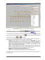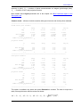
1
Software PHOTOMOD 4.4 Module PHOTOMOD Solver USER MANUAL Racurs, Moscow, 2009 1. PHOTOMOD Solver. Module of the block adjustment ....................................................... 5 2. Installation and starting ........................................................................................................ 5 3. Adjustment of projects of different types ........................................................................... 5 4. Coordinate systems .............................................................................................................. 6 5. Free model.............................................................................................................................. 7 6. Source window ...................................................................................................................... 7 6.1 Points displaying...................................................................................................................... 8 6.2 View parameters...................................................................................................................... 9 6.3 Points selection by filter ......................................................................................................... 10 6.4 Points window ........................................................................................................................ 11 6.5 Images window ...................................................................................................................... 12 6.6 Stereopairs window ............................................................................................................... 13 6.7 Information window on the Source tab .................................................................................. 13 6.8 Images, stereopairs and strips displaying ............................................................................. 15 6.9 Cursor modes ........................................................................................................................ 15 6.10 Graphic windows toolbar ....................................................................................................... 16 7. Methods of block adjustment ............................................................................................. 17 8. Parameters window ............................................................................................................. 17 8.1 Coordinate system tab........................................................................................................... 17 8.2 Adjustment tab ....................................................................................................................... 18 8.2.1 Independent strips method .................................................................................................... 19 8.2.2 Independent stereopairs method........................................................................................... 20 8.2.3 Bundle adjustment ................................................................................................................. 20 8.2.4 Systematic error compensation ............................................................................................. 21 8.3 Report tab .............................................................................................................................. 23 9. Computations....................................................................................................................... 33 10. Stereopairs tab..................................................................................................................... 35 10.1 Error vectors displaying ......................................................................................................... 35 10.2 Residuals window .................................................................................................................. 36 10.3 Brief residuals report on Stereopairs tab ............................................................................... 37 Solver July 25, 2009 10.4 Tie residuals window ............................................................................................................. 38 10.5 Information window on the Stereopairs tab ........................................................................... 40 10.6 Editing points ......................................................................................................................... 42 11. Images tab ............................................................................................................................ 46 11.1 Residuals window .................................................................................................................. 47 11.2 Residuals on image ............................................................................................................... 48 11.3 Brief residuals report on the Images tab................................................................................ 49 11.4 Information window on the Images tab.................................................................................. 49 12. Report creation .................................................................................................................... 50 13. Console window .................................................................................................................. 52 14. Saving the block scheme.................................................................................................... 52 15. Finishing the work in PHOTOMOD Solver ........................................................................ 52 16. Block adjustment by external programs ........................................................................... 52 17. Single aerial image adjustment .......................................................................................... 55 18. Adjustment of scanner monoblock and stereoblock....................................................... 57 Appendix A. Exterior orientation angular systems ......................................................................... 65 Appendix B. Recommendations on aerial images blocks adjustment in PHOTOMOD system.. 67 1. Typical errors ....................................................................................................................... 67 2. Stages of control ................................................................................................................. 67 2.1 Interior orientation control ...................................................................................................... 67 2.1.1 Interior orientation control. PHOTOMOD AT module ............................................................ 67 2.2 Relative orientation control .................................................................................................... 67 2.2.1 Points recognition control. PHOTOMOD AT, AAT modules.................................................. 67 2.2.2 Control of uniform distribution of points measurements on stereopairs. PHOTOMOD AT, AAT modules ......................................................................................................................... 68 2.2.3 Control of vertical parallaxes on stereopairs. PHOTOMOD AT, AAT modules .................... 68 2.3 Control of triplets.................................................................................................................... 68 2.3.1 Control of uniform distribution of points measurements in triplets. PHOTOMOD AT, AAT modules ................................................................................................................................. 68 2.3.2 Control in triplets. PHOTOMOD AT, AAT modules ............................................................... 69 2.3.3 One strip adjustment in free model using independent models method. PHOTOMOD Solver module ................................................................................................................................... 69 2.4 3 Control of free model adjustment .......................................................................................... 69 RACURS Co., Ul. Yaroslavskaya, 13-A, office 15, 129366, Moscow, Russia PHOTOMOD 4.4 2.4.1 Using of splitting on sub-blocks. PHOTOMOD Solver module ............................................. 69 2.4.2 Detection of blunders in camera focus input. PHOTOMOD Solver module.......................... 69 2.4.3 Detection of blunders in strips tying. PHOTOMOD Solver module ....................................... 70 2.4.4 Intermediate control of tie measurements blunders. PHOTOMOD Solver module............... 70 2.4.5 Blunders detection on interstrip not-transferred points. PHOTOMOD Solver module .......... 70 2.4.6 How to detect errors of tie points measurements. PHOTOMOD Solver module .................. 70 2.4.7 How to detect errors of automatic tie points measurements. PHOTOMOD Solver module.. 71 2.5 Control of adjustment of georeferenced blocks..................................................................... 72 2.5.1 How to detect a reference to wrong coordinate system. PHOTOMOD Solver module......... 72 2.5.2 Detection of blunders in GCP measurements. PHOTOMOD Solver module ....................... 72 2.5.3 Selection from several adjacent GCP, if their error' vectors have opposite direction. PHOTOMOD Solver module.................................................................................................. 72 2.5.4 Control of GCP located on one stereopair. PHOTOMOD Solver module ............................. 73 2.5.5 Control of adjustment with projection centers. PHOTOMOD Solver module ........................ 73 2.5.6 Detection of systematic errors of interior orientation. PHOTOMOD Solver module ............. 73 2.5.7 Bundle adjustment and adjustment import: errors on points measured on one stereopair. PHOTOMOD Solver module.................................................................................................. 74 2.6 Control during points filtering in PHOTOMOD Solver ........................................................... 75 2.6.1 Irregularity of points' distribution control. PHOTOMOD Solver module ................................ 75 3. Bundle adjustment specific features................................................................................. 75 4. Interpretation of errors shown in PHOTOMOD Solver on Stereopairs and Images tabs 75 5. Processing of survey with big images overlap ................................................................ 76 6. Recommendations on long-focus camera survey ........................................................... 76 7. Tie points measuring in forested areas, in areas with bad stereo effect. Tie points measuring between strips acquired in different seasons .............................................................. 77 8. © 2009 Tie points measuring on lengthy objects boundaries ..................................................... 77 4 Solver July 25, 2009 1. PHOTOMOD Solver. Module of the block adjustment PHOTOMOD Solver program is used to adjust strips and blocks of aerial or satellite images. The source images must be previously processed in PHOTOMOD AT module (see PHOTOMOD AT User Manual). Besides, you can export and import data from/to PHOTOMOD Solver module to/from external software of data adjustment, see the chapter 16 Block adjustment by external programs. 2. Installation and starting PHOTOMOD Solver module is a part of PHOTOMOD system and is installed by setup.exe file from your installation CD. See also readme.txt file on this CD for the installation instructions. PHOTOMOD Solver is started for the selected project from the PHOTOMOD Montage Desktop program (see the corresponding User Manual). Note that the project must be completely prepared in PHOTOMOD AT module. If necessary, you can also adjust a part of block. Use Block editor window in Montage Desktop module to select sub-block of images intended for further adjustment. See details in PHOTOMOD Montage Desktop User Manual. 3. Adjustment of projects of different types PHOTOMOD system works with two types of projects (based on the source image geometry) – Central projection (images obtained by photo cameras) and Scanner images (images obtained by scanning devices such as SPOT, ASTER, IRS, IKONOS etc.). The project type is selected in PHOTOMOD Montage Desktop module during project creating (see the corresponding User Manual). While processing central projection images (acquired by photo camera) PHOTOMOD works with images block (Block project subtype) or single image (project subtype Single image). See the chapter 17 Single aerial image adjustment for the description of single images adjustment. The process of adjustment for blocks of airborne images is performed as described in chapters 6-18 of present User Manual. 5 RACURS Co., Ul. Yaroslavskaya, 13-A, office 15, 129366, Moscow, Russia PHOTOMOD 4.4 Fig.1 Project type selection Projects of the Scanner survey type are divided on two sub-types – Monoblock and Stereoblock. If the set of scanner images has minimal overlap and does not form a stereopair, you should create new PHOTOMOD project as Monoblock type. Single scanner image is processed in project of Monoblock type too. Details on project types and formats of processed images see in PHOTOMOD Montage Desktop User Manual. In case of stereopair or set of stereopairs of space images, they are processed as Stereoblock project type, see the chapter 18 Adjustment of scanner monoblock and stereoblock. Images acquired by airborne digital sensor ADS 40 by Leica Geosystems, Swizerland, are processed in PHOTOMOD system as described in PHOTOMOD Montage Desktop User Manual. 4. Coordinate systems The coordinate system can be selected either in PHOTOMOD Montage Desktop module during the project creation, or in PHOTOMOD Solver while the block adjustment. Refer to PHOTOMOD Montage Desktop User Manual for full description of coordinate systems and map projections supported by PHOTOMOD system. In some cases images orientation and their further processing in PHOTOMOD system modules are executing without images referencing to ground control points (without referencing to coordinate system, that corresponds the “free model” term, see the chapter 5 Free model). © 2009 6 Solver July 25, 2009 5. Free model If you have no ground control points at the beginning of work with the project you can build “free model”. In this case you make the interior orientation and tie points measurements in PHOTOMOD AT module. PHOTOMOD Solver builds a model based only on tie points and calculates tie errors. Then you can pass to Block processing stage in PHOTOMOD Montage Desktop, build DTM’s in PHOTOMOD DTM and create 3D vectors in PHOTOMOD StereoDraw. Thus when you will get coordinates of control points, the biggest part of job is already done. Once you have GCP you should go back to Aerial triangulation stage and measure them on images, then pass to the Block adjustment stage and adjust the block again in PHOTOMOD Solver. After passing the Block processing stage all your TINs and 3D vectors will be transformed to the selected geodetic coordinate system automatically. To adjust block in free model select the option Free model in Parameters | Adjustment window and set the approximate aerial survey basis in units of coordinate system of a project (meters, feet, etc., in Basis field). Free model errors are displayed in the same units and depend on the basis accuracy. Note. There is no way to create orthomosaic and contour lines in free model 6. Source window of Once PHOTOMOD Solver is started for the project at the first time (using the button the PHOTOMOD Montage Desktop program), Block adjustment window is opened and the source data, collected in the PHOTOMOD AT module, is loaded automatically to the window of the Source tab. When adjustment is completed you get three tabs in the graphic window: Source, Stereopairs and Images. First of them shows the initial images block (see Fig.1), the second and the third ones – the block adjusted with residual’s vectors, that makes easy visual analysis of adjustment results. After adjustment procedure the block scheme is shown on the Stereopairs tab of the main window (see the chapter 10 Stereopairs tab), and also on the third tab Images, see the chapter 11 Images tab. 8 In the upper part of PHOTOMOD Solver window there are main buttons that allow to perform the adjustment procedure: • – opens the window for adjustment parameters setting (see the chapter 8 Parameters window) • – starts the process of computing of exterior orientation parameters and coordinates of all points of a block (see the chapter 9 Computations) • – opens the window with adjustment results (see the chapter 12 Report creation) • • 7 – saves the adjustment results that allows to proceed to next project processing stage in PHOTOMOD system (see the chapter 15 Finishing the work in PHOTOMOD Solver) – exits PHOTOMOD Solver module RACURS Co., Ul. Yaroslavskaya, 13-A, office 15, 129366, Moscow, Russia PHOTOMOD 4.4 Fig.2 Initial block state on the Source tab If some errors occur while image block loading you will receive an appropriate message and further work in the module will be blocked. If the source dataset is loaded successfully the Parameters button becomes available. You have to set process parameters if you start Block adjustment for the first time (see the chapter 8 Parameters window). Parameters are memorized when exiting PHOTOMOD Solver module and restored for each future block adjustment session. Borders of selected images, stereopairs and strips are shown in lighter color. 6.1 Points displaying Points are shown on block scheme by graphic symbols. Point type is shown by the color and shape of symbol as follows: • points with known coordinates (control and check): - XYZ points – double triangle XY points – single triangle; Z points – circle; ground control – red color check – black color; - rejected from adjustment – white color ; • projection centers – small black square • tie points © 2009 ; ; measured on at least one stereopair – small diagonal cross 8 Solver July 25, 2009 - measured on no stereopairs – small circle - measured on only one stereopair – black color - measured on more than one stereopair on one strip – green color (for example, measured in triplet) - interstrip point – deep blue color - rejected from adjustment – white color measured on only one image on one strip – magenta color (light magenta if rejected) - ground point (tie point that is not targeted and is not a projection center) – no symbol; targeted point – bold symbol (one of described above) ; - (light blue if rejected); Any point can be displayed using a set of symbols. For example, control XYZ point, identified on two strips (in the overlap areas) is displayed as double red triangle and blue diagonal cross . All projection centers except the first and last ones are displayed as a square and a diagonal cross . The white circle shows selected points. Symbols for points displaying are also described in the chapter 6.3 Points selection by filter. 6.2 View parameters The window View parameters (opened by the icon ) is used to select the elements to be included to the block scheme. The window is divided into five main panes, related to displaying points, images, stereopairs, strips and the map grid respectively. Fig.3 View parameters 9 RACURS Co., Ul. Yaroslavskaya, 13-A, office 15, 129366, Moscow, Russia PHOTOMOD 4.4 • Points panel - Show / all – all points measured on the images of the block are displayed. - Show / filter – points to be displayed are selected according to filter settings. Click the Parameters button (if the Filter option is selected) to open a window used for setup point’s filter, see the chapter 6.3 Points selection by filter. Thus, points selected in this window are visualized in viewing window. - Names – defines which points will be displayed with labels (options All, Selected, None). • Images panel - Show – shows / hides image borders. - Names – defines which images will be displayed with labels (options All, Selected, None). • Stereopairs panel - Show – shows / hides borders of stereopairs. - Names – defines which stereopairs will be displayed with labels (options All, Selected, None). • Strips panel - Show – shows / hides borders of strips. - Names – defines which strips will be displayed with labels (options All, Selected, None). • Grid panel – allows to show map grid lines (lines) and coordinates (coordinates). 6.3 Points selection by filter ) is used to filter and select points The dialog Selection by filter (opened by the icon based on some criteria and to show selected points using symbols on block scheme. The symbols are described in the chapter 6.1 Points displaying. Fig.4 “Point selection” window © 2009 10 Solver July 25, 2009 There are five panels, used to setup different criteria: • By coordinates. List of point types used to select/deselect points includes: − ground control – ground control points, projection centers − check – check points, projection centers − rejected ground – points excluded from adjustment, with known coordinates (ground control, check and projection centers, both in plane and height (3D), plane (horizontal) and height (vertical)), − no coordinates – points with unknown coordinates (tie, targeted and projection centers (if their coordinates are not known)) • By ties − single – tie points measured on no stereopairs − stereopair – tie points measured at least on one stereopair − triplet – tie points measured at least on one triplet − strip tie – tie points measured in strips overlap − non-transferred – tie points not measured on the adjacent images − used – tie point used for the block adjustment as ties − rejected – tie point rejected from the block adjustment as ties • Auxiliary − geodetic – tie points that are neither targeted nor projection centers − targeted – targeted points − projection centers – projection centers − with changed type – points which type was changed in PHOTOMOD Solver • By residual value − worst points – selection of points with maximum residual values. Number of “worst” points is to be set in corresponding text field. − over acceptable residuals – selection of points with residual values greater than the Acceptable residual parameter, indicated in the Parameters window, on the Report tab, in Acceptable residuals panel, see the chapter 8.3 Report tab. You can set on ground and/or tie options to select ground and/or tie points that satisfy chosen criteria as well as XY and Z options to take into account XY and/or Z residuals only. • In selected models − all select points, which belong to all models − at least one select points, which belong to at least one model • Also invisible – mark the option to select both visible and invisible points. If the option is not marked, only visible points will be selected. Points may be invisible, if they do not satisfy to preset filter of points displaying. Note. The panel By residual value is inactive if the window is opened from the Source tab but is used on the Stereopairs and Images tabs The buttons Select, Add, Toggle and Subtract are used to execute the appropriate selection operations with selected points. 6.4 Points window Points window (opened by the icon the block scheme by their names. 11 point list) is used for quick selection of points in RACURS Co., Ul. Yaroslavskaya, 13-A, office 15, 129366, Moscow, Russia PHOTOMOD 4.4 Fig.5 Points window At the upper part of the window there is a text field, where you can type the point name to be searched and selected. You can also select point in the point list below (sorted in alphabetical order). If the Auto option is on, selected point is automatically marked in the block scheme (outlined by the white circle ). If you need to select several points, turn off the Auto option and use the Select button for point’s selection. If current point is already selected, click the Select button to cancel point selection. The option List of selected objects is used to show a list of currently selected objects. 6.5 Images window image list) is used for quick selection of images in Images window (opened by the icon the block scheme by their names. At the upper part of window there is a text field, where you can type the image name to be searched and selected. You can also select image in the image list below (sorted in alphabetical order). If the Auto option is on, selected image is automatically marked in the block scheme (bordered by yellow bold line). If you need to select several images turn off the Auto option and use the Select button for images selection. If current image is already selected, click the Select button to cancel image selection. The option List of selected objects is used to show a list of currently selected objects. © 2009 12 Solver 6.6 July 25, 2009 Stereopairs window stereopair list) is used for quick selection of Stereopairs window (opened by the icon stereopairs in the block scheme by their names. At the upper part of window there is a text field, where you can type the stereopair name to be searched and selected. You can also select stereopair in the list below (sorted in alphabetical order). If the Auto option is on, selected stereopair is automatically marked in the block scheme (bordered by light-blue bold line). If you need to select several stereopairs, turn off the Auto option and use the Select button for stereopairs selection. If current stereopair is already selected, click the Select button to cancel stereopair selection. The option List of selected objects is used to show a list of currently selected objects. 6.7 Information window on the Source tab point attributes) is used to view the attributes Information window (opened by the icon of currently selected point: its type, coordinates and measurements. There is a text field at the upper window part, which shows the name of selected point, if the only one point is selected. Mark the option Editing panel to open the panel allowing to change point type (control or check and vice versa), and also to exclude points from the adjustment. Current point’s type is indicated by marked check box near the appropriate type name in this panel. To change the type of the selected point for the next adjustment, push one of the appropriate buttons: - control - check - rejected as a ground control or check point, but can be used as a tie You can edit control point coordinates using the window opened by the button (Edit coordinates), which is used to open the window for editing coordinates of triangulation points, described in the chapter 10.6 Editing points. 13 RACURS Co., Ul. Yaroslavskaya, 13-A, office 15, 129366, Moscow, Russia PHOTOMOD 4.4 Fig.6 Information window shows the data for selected point Panel By ties contains the button (Edit tie points), used for tie points editing in special window. See the chapter 10.6 Editing points. You can exclude tie point selected from the further adjustment by the button excluded tie point to adjustment push the button restoring push the buttons and . To restore . For ground control and check points accordingly). The rest part of the Information window is used to display selected point attributes. It contains information if the only one point is selected in graphic window. − Geodetic. Shows initial (“real”) coordinates entered in PHOTOMOD AT module (reference coordinates) and also initial weights of coordinates (reference weights). − Ties. Used to show information about tie points. Images – number of images, where the point is measured, and measurements of the point (its coordinates) in these images, number of stereopairs and strips. − Type – indicates whether the point was ground control, check or rejected during adjustment, and whether it used as a tie. It also indicates is the point a projection center, and shows point code (or image code for projection centers) − Images – list of images the point was measured on − Stereopairs – list of stereopairs the point was measured on − Strips – list of strips the point was measured on (on one image at least). The window allows to select images, stereopairs and strips where the point is measured, in the following way. © 2009 14 Solver July 25, 2009 Holding Ctrl key pressed you can click the following lines in the window: Tie→images, Tie→images→image name, Images, Images→image name, Stereopair, Stereopairs→stereopair name, Strips, Strips→strip name. At that the appropriate object or object group will be highlighted. If the object is already selected, the selection will be cancelled. If Shift key is pressed down the selection will be inverted. 6.8 Images, stereopairs and strips displaying Images, stereopairs and strips are shown on the block scheme in the following way: • • • Images are shown by yellow frames, selected images – by light yellow frames Stereopairs (images overlap areas) – by blue frames Strips (the whole areas of coverage of strip's images) – by magenta frames. Models and images names can also be displayed if the names option in View parameters window is on (see the chapter 6.2 View parameters). 6.9 Cursor modes select mode is Selection mode is the default cursor mode (is on when the button pushed). You can define the type of objects to be selected by following icons: Select points , Select images and Select models . Click the object neighborhood to select a closest object (the screen distance between the cursor and the object should be less than the cursor size). Note. Points are selected by their centers, images, stereopairs and strips – by their frames By default, selection of objects cancels the selection of previously selected ones (if they were selected in Points selection, Images selection and Model selection modes). All other objects (if any) remain selected, since there is a possibility of using objects filter that depends on selected objects (see the chapter 6.4 Points window). To add objects to selection, select them by mouse along with pressed down Ctrl key. In this case the cursor gets “plus” sign added . To deselect some objects press and hold Shift key. In this case the cursor gets “minus” sign added . To invert selection of the group of objects press and hold down Shift and Ctrl keys. At that, the cursor gets “minus-plus” sign added blank part of the window or push upper menu button objects. Pan mode is activated by pushing the Pan icon Space bar if you are in Select mode (when the button . Click the (Unselect objects) to unselect all or by pressing and holding down the is pushed). Once the pan mode is on, small pictogram with arrows appears nearby the cursor . There are following options in the pan mode: - panning the image (the default one). Press and hold mouse button to pan over the image. 15 RACURS Co., Ul. Yaroslavskaya, 13-A, office 15, 129366, Moscow, Russia PHOTOMOD 4.4 - - zoom in. Press Ctrl key to zoom in the image using the zoom box (drawn by the mouse). Mouse click causes two times image enlarging. Or press and hold Ctrl-Space shortcut if you are in Selection mode (when the button is pushed). zoom out. Press Shift or Alt keys to zoom out the image in the same way as described above. Or press and hold Shift-Space or Alt-Space if you are in Selection mode (when the button is pushed). 6.10 Graphic windows toolbar Graphic windows toolbar contains the following buttons: • Source scale – to go back to original block scheme zoom • Zoom in (duplicated by “*” key) – turns on the mode which allows to enlarge the block scheme twice by each mouse click • Zoom Out (duplicated by “/” key) – turns on the mode which allows to reduce the block scheme twice by each mouse click • Pan mode – allows to pan the block scheme by mouse. See the chapter 6.9 Cursor modes • Select mode – turns on selection mode for points, images, stereopairs and strips. See the chapter 6.9 Cursor modes • Select points – allows to select points. See the chapter 6.1 Points displaying • Select images – allows to select images. See the chapter 6.8 Images, stereopairs and strips displaying • Select models – allows to select stereopairs and strips. See the chapter 6.8 Images, stereopairs and strips displaying • Selection by filter – opens/closes a dialog used to filter and select points (see the chapter 6.3 Points selection by filter) • Unselect objects – cancels all selection • Marker parameters – opens dialog used to change cursors’ shape, size and color. • View parameters – opens a dialog used to set view parameters (see the chapter 6.2 View parameters) • Residuals – opens a dialog used to set parameters of residuals viewing. See the chapter 10.2 Residuals window, 11.1 Residuals window. Available only on the Stereopairs and Images tabs. • Point list – opens/closes a window with a point list (see the chapter 6.4 Points window) • Point attributes – opens/closes a window with the information, related to selected point. See the chapter 6.7 Information window on the Source tab, 10.5 Information window on the Stereopairs tab, 11.4 Information window on the Images tab. • Points residuals – opens / closes a window for displaying error vectors on selected tie point (see the chapter 10.4 Tie residuals window). Available only on the Models tab. © 2009 16 Solver July 25, 2009 • - Image residuals – opens / closes a window for displaying error vectors on selected image (see the chapter 11.2 Residuals on image). Available only on the Images tab • Image list – opens/closes Images window with an image list (see the chapter 6.5 Images window) • Stereopair list – opens/closes Stereopairs window with a model list (see the chapter 6.6 Stereopairs window) • Residuals window – opens/closes a window containing RMS, mean absolute and maximum adjustment error values. Used for quick estimation of the adjustment results without opening a full report. Differs for Stereopairs and Images tabs (and is available only on these tabs). See the chapter 10.3 Brief residuals report on the Stereopairs tab and 11.3 Brief residuals report on the Images tab • • Hide windows – closes all additional windows Save block scheme to the vector (wmf) or raster (bmp) format. See the chapter 14 Saving the block scheme. 7. Methods of block adjustment PHOTOMOD Solver provides three algorithms to be used for the block adjustment procedure: Independent strips, Independent stereo pairs and Bundle adjustment. • • • Independent strips. This method is used to check out the gross errors, such as wrong coordinate values of control points, incorrect tie point's measurements, etc. Accuracy of this method in case of long strips (more than 10 images) may be dozen times worse than adjustment accuracy achieved by the other two methods. See method setup parameters in the chapter 8.2.1 Independent strips method Independent stereo pairs. Use this method to increase the accuracy, you have achieved by Independent strips method, and to detect more delicate errors and possibly for final adjustment. See method setup parameters in the chapter 8.2.2 Independent stereopairs Bundle adjustment is used for the final block adjustment. See details about method setup in the chapter 8.2.3 Bundle adjustment. In most cases, it is practical to perform adjustment alternately by method of independent stereopairs and bundle adjustment for searching and correction of delicate errors. You can select adjustment method and setup it on the Adjustment tab of the Parameters window opened by pushing the button , see the chapter 8.2 Adjustment tab. 8. Parameters window Parameters window opens after clicking the button report parameters) and includes the following tabs: 8.1 (Edit adjustment and Coordinate system tab The Coordinate system tab is used to select the project coordinate system (see the chapter 4 Coordinate systems for details). Push the Change button and select coordinate system and projection in standard PHOTOMOD window, see Montage Desktop User Manual. After 17 RACURS Co., Ul. Yaroslavskaya, 13-A, office 15, 129366, Moscow, Russia PHOTOMOD 4.4 choosing or changing the coordinate system and map projection for images block processing you can adjust the block. 8.2 Adjustment tab The Adjustment tab is used to select the Block adjustment method: Independent strips, Independent stereopairs or Bundle adjustment (see the chapter 7 Methods of block adjustment). Use Free model adjustment mode to adjust a block without GCP, and to provide following georeference. The Free model option is used this procedure (see the chapter 5 Free model). Fig.7 Adjustment parameters Free model adjustment is executed using distance between projection centers, indicated in Basis field (in units of coordinate system of a project). Basis value by default is 1000. You can reject the worst tie points during adjustment automatically, using filtering options on the Tie point rejection panel: worst points (number of points with maximal residuals) and over acceptable residuals (all points with residuals exceeded the accepted values indicated in Acceptable residuals panel on Report tab, see the chapter 8.3 Report tab). If the options are on, filtered points will be excluded from adjustment. When the adjustment method is selected you can setup it in the window, opened by the button Method parameters, see the chapter 8.2.1 Independent strips method, 8.2.2 Independent stereopairs method, 8.2.3 Bundle adjustment. Systematic errors of adjustment are considered, and you can setup their compensation parameters in the window opened by the button Systematic error compensation, see the chapter 8.2.4 Systematic error compensation. © 2009 18 Solver 8.2.1 July 25, 2009 Independent strips method When you have selected independent strips method of adjustment, you can setup the process parameters in the window opened by the button Method parameters on the Adjustment tab (see the chapter 8.2 Adjustment tab). Fig.8 Independent strips method setup The following parameters are available: Equation weights for ground control, tie points and projection centers with specified coordinates. You can reduce the residuals values by changing the equation weights. However, real adjustment accuracy can be also reduced in this case. In many cases the weight value of 1 is near to optimal. You have to have check points enough to control the result of optimal value search. If there is a lack of check points you can temporarily transfer some GCP to check. The decimal delimiter is "." (period). The exponent sign is "e". Example: "5.7e-4" = 0.00057. The slider Adjustment accuracy is used to setup relative accuracy, and when it is reached the iteration process of adjustment may be completed. You are recommended to use the default value 0.5. When it is 0.5-0.55, the adjustment process converges and provides an optimal ratio accuracy-time. If you increase the value, the accuracy generally does not improve considerably, but processing time may increase very much up to infinite looping of iterations (in this case you may stop iterations when you need using the Stop button). If the accuracy value is less then 0.5 the adjustment time is reducing due to accuracy decreasing. The algorithm of optimization has a complex nature, that is why the dependence of adjustment time and accuracy from this parameter value is nonlinear. Mark the option Calculate relative orientation to recalculate relative orientation parameters during block adjustment. When processing close range photogrammetry projects, containing points with big differences in x-parallaxes, the option Maximum distance (in bases) is used. Points located from projection centers on the distance more then indicated in this field are excluded from adjustment on each stereopair automatically. The distance is input in survey bases, i.e. if stereopair basis is 10 m and in this field the value 100 is set up, then the points located farther then 1000 m from projection centers will be excluded. It is recommended to set up the values not more than 100, because when the points with distance more than 100 survey bases are used for adjustment, the method of independent strips (or stereopairs) would fail or return a blunder result. Basically (if there are no blunders in measurements), reduction of this value leads to decreasing of RMS for the whole block. However if too small value is set up, there will be 19 RACURS Co., Ul. Yaroslavskaya, 13-A, office 15, 129366, Moscow, Russia PHOTOMOD 4.4 very few tie points (or no points at all) in triple overlap, that will result in adjustment error with an appropriate message. 8.2.2 Independent stereopairs method Parameters of independent stereopairs method are setup similarly to those of independent strips method (see the chapter 8.2.1 Independent strips method). However, there is a possibility to choose the algorithm of adjustment optimization in the following way. Fig.9 Independent stereopairs method setup In settings window there is the Optimization algorithm panel, that allows to select one of the following methods of adjustment optimization: Gradient (by default) and Matrix inversion. The last method was used in previous (up to 4.1 inclusive) versions of PHOTOMOD system. It was developed for moderate blocks of images (less than 500 images). 8.2.3 Bundle adjustment When using bundle adjustment method you can setup its parameters in the window opened by pushing the button Method parameters on the Adjustment tab, see the chapter 8.2 Adjustment tab. Fig.10 Bundle adjustment setup © 2009 20 Solver July 25, 2009 The panel Measurement precision (RMS) is intended for setup of the following parameters: • image measurements – mean square accuracy of points recognition on images (which is performed in PHOTOMOD AT module or in point editing window, see the appropriate User Manual). It is measured in camera units: mm or pixels. This accuracy depends on the quality of photomaterial (photographic grain, blur, image deformations that were not considered in camera parameters, including geometric distortions of scanner) and on accuracy of recognition performed automatically or by operator. In case of operator the main impact make visual acuity, terrain type, image zoom at recognition, carefulness of work. For automatic recognition settings of automat and terrain type are important. If scanning resolution of image corresponds to image's quality, and points are recognized properly, this value has to be between 0.5–1.0 of pixel size. • ground control points, projection centers – mean square accuracy of GCP coordinates and projection centers that are used as GCP. It is measured in units of selected coordinate system of a project (meters, ft. etc.). This accuracy depends on the measuring equipment. • exterior orientation angles (omega, phi, kappa) – mean square accuracy of exterior orientation angles that are used as GCP data. It is measured in degrees. This accuracy depends on the measuring equipment. Mark the option Use exterior orientation angles to use exterior orientation angles during adjustment procedure. 8.2.4 Systematic error compensation For automatic calculation and compensation of some systematic errors of block adjustment you can use settings in a window opened by the button Systematic error compensation on the Adjustment tab, see the chapter 8.2 Adjustment tab. Fig.11 21 RACURS Co., Ul. Yaroslavskaya, 13-A, office 15, 129366, Moscow, Russia PHOTOMOD 4.4 In the Projection center coordinates (GPS) panel you can select a type of compensation applied to projection center coordinates (GPS). If the airborne survey was performed using GPS equipment, for measuring the projection centers coordinates, you can calculate the corrections to these coordinates during adjustment, by choosing the appropriate option in the Compensation type panel. Usually the corrections of GPS device, which were introduced on strip survey should be considered. So it is recommended to turn on the option common for strip. Calculated corrections of coordinates measured by GPS could be included into adjustment report, see the chapter 8.3 Report tab. Coordinates corrections for projection centers are calculated by ground control points and are as follows: ΔX = G0x + G1x · N ΔY = G0y + G1y · N , ΔZ = G0z + G1z · N where N — number of image in block or strip, G — polynomial coefficients that are calculated during adjustment. If polynomial order equals 1 (input in the Polynomial degree panel), then both G0, and G1 are used, if the order is 0, then just G0 are used, and G1 are assumed to be equal 0. The panel Exterior orientation angles is used to setup the type of corrections that are applied to exterior orientation angles of images, if they are in the project and are used for adjustment. These parameters are available only for bundle adjustment method and are as follows: =A =A , =A where A — coefficients calculated during adjustment. The type of polynomial corrections for adjustment results is setup in the Polynomial corrections for block panel: XY, Z, XYZ (at user's option). The panel is available only for methods of independent strips and independent stereopairs. Polynomial corrections are calculated using the following formulas: ΔX = Ax + B x X + C xY + D x X 2 + E x XY + Fx Y 2 ΔY = Ay + B y X + C y Y + D y X 2 + E y XY + Fy Y 2 . ΔZ = Az + B z X + C z Y + D z X 2 + E z XY + Fz Y 2 A• , …, F• coefficients are calculated during post-processing of adjustment results performed by GCP (including projection centers). Corrections obtained are added to adjusted coordinates of all points of the block, including projection centers. In most cases you are recommended to turn off polynomial corrections usage. © 2009 22 Solver 8.3 July 25, 2009 Report tab The Report tab is used to select adjustment report parameters and parameters of residuals visualization on the block scheme (acceptable residuals and method of tie residuals calculating). Fig.12 Report parameters The Include in the report panel allows you to include the following values to the report. Residuals – the option allows to include the section with adjustment residuals into the report: ----------------------------------------------------------------------------------------------------------------------------------------------------------------------Estimation of block adjustment accuracy Unacceptable residuals are marked with "*". ----------------------------------------------------------------------------------------------------------------------------------------------------------------------Generalized adjustment residuals information Sigma_0 = 0.623 ----------------------------------------------------------------------------------------------------------------------------------------------------------------------- Sigma_0 value is calculated only for bundle adjustment method. It is calculated using the following formula: ⎛ Nt ⎡⎛ im ⎞ 2 ⎛ im ⎞ 2 ⎤ N g ⎡⎛ ΔX ig 1 ⎜ ⎢⎜ Δxi ⎟ ⎜ Δy i ⎟ ⎥ ⎜ ⎢ σ = + + ∑ ∑ ⎜ g ⎟ N t + N g ⎜⎜ i=1 ⎢⎜⎝ s x,imi ⎟⎠ ⎜⎝ s im i=1 ⎢⎝ s X,i y,i ⎠ ⎥ ⎣ ⎦ ⎝ ⎣ im g where Δx , Δy im — residuals on images, ΔX , 2 0 2 ⎞ ⎛ ΔYi g ⎟ +⎜ g ⎟ ⎜ s ⎠ ⎝ Y,i 2 ⎞ ⎛ ΔZ ig ⎟ +⎜ g ⎟ ⎜ s ⎠ ⎝ Z,i ⎞ ⎟ ⎟ ⎠ 2 ⎤⎞ ⎥⎟ , ⎥ ⎟⎟ ⎦⎠ ΔY g , ΔZ g — residuals on GCP and im im im projection centers (GPS), s xim , s im y , s X , sY , s Z — corresponding to measurements 23 RACURS Co., Ul. Yaroslavskaya, 13-A, office 15, 129366, Moscow, Russia PHOTOMOD 4.4 accuracy a priori, N t — number of points measurements on images (point-image pairs), N g — number of GCP and projection centers. More details about Sigma parameter see in the chapter 10.3 Brief residuals report on the Stereopairs tab. Control, check – allows to include a section with ground control and check points residuals: -----------------------------------------------------------------------------------Ground control point residuals N Xm-Xg Ym-Yg Zm-Zg 8801 ... 9693 0.157 -0.0726 -0.00749 0.173 -0.0175 0.0538 -0.00214 0.0566 mean absolute: 0.0781 RMS: 0.105 maximum: 0.157 number of points (differences): 4 ( 4 0.0347 0.0456 0.0726 0.00338 0.00436 0.00749 4 4 Xm-Xg Ym-Yg Zm-Zg mean absolute: 0.00 RMS: 0.00 maximum: 0.00 number of points (differences): 0 ( 0 0.00 0.00 0.00 0.00 0.00 0.00 0 0 Exy (m) 0.0920 0.114 0.173 4) projection centers N Exy (m) ... 0.00 0.00 0.00 0) -----------------------------------------------------------------------------------Check points residuals N Xm-Xg Ym-Yg Zm-Zg Exy (m) *212 ... 8822 0.989 1.67 -1.02 1.94 -0.0833 -0.0645 0.445 0.105 mean absolute: 0.394 RMS: 0.515 maximum: 1.44 number of points (differences): 23 ( 22 0.528 0.729 1.69 1.57 1.84 3.61 0.750 0.893 1.94 22 22 22) projection centers N Xm-Xg Ym-Yg Zm-Zg Exy (m) 199 ... 264 -1.17 0.449 -1.24 1.26 -0.943 0.515 -2.38 1.07 mean absolute: 1.05 RMS: 1.05 maximum: 1.17 number of points (differences): 3 ( 3 0.516 0.518 0.583 35.3 59.1 102. 1.17 1.17 1.26 3 3 3) ------------------------------------------------------------------------------------ The option is available only when the option Residuals is marked. The data is output as a table, where point name and its values are shown: ΔX = X m − X g , ΔY = Ym − Yg , ΔZ = Z m − Z g , E xy = © 2009 (ΔX )2 + (ΔY )2 , 24 Solver July 25, 2009 where X m , Ym , Z m — coordinates of adjusted (mean) point position, X g , Yg , Z g — user defined coordinates. On stereopairs – allows to include a section with adjustment residuals on points measured on one stereopair at least. The option is available only when the option Residuals is marked. Depending on the Tie residuals radio button the report contains the following statistical parameters. When the option Tie residuals—From mean value is selected: ΔX ij = X ij − X m , ΔYij = Yij − Ym , ΔZ ij = Z ij − Z m , E xy,ij = (ΔX ) + (ΔY ) 2 2 ij ij , where i — point number, j — stereopair number, X ij , Yij , Z ij — coordinates of i point, calculated from j stereopair; are shown correspondingly in X-Xср, Y-Yср, Z-Zср and Exy columns: -----------------------------------------------------------------------------------Tie point residuals (from mean) N X-Xm Y-Ym Z-Zm mean absolute: 0.103 RMS: 0.134 maximum: 0.510 number of points (differences): 53 ( 122 0.0759 0.0986 0.414 0.149 0.195 0.849 122 122 Exy (m) 0.139 0.166 0.516 122) -----------------------------------------------------------------------------------Targeted point residuals (from mean) N X-Xm mean absolute: 0.00 RMS: 0.00 maximum: 0.00 number of points (differences): 0 ( 0 Y-Ym Z-Zm Exy (m) 0.00 0.00 0.00 0.00 0.00 0.00 0 0 0.00 0.00 0.00 0) -----------------------------------------------------------------------------------Tie point residuals - projection centers (from mean) N X-Xm mean absolute: 0.00 RMS: 0.00 maximum: 0.00 number of points (differences): 9 ( 18 Y-Ym Z-Zm 2.53e-14 1.07e-13 4.55e-13 0.00 0.00 0.00 18 18 Exy (m) 2.53e-14 1.07e-13 4.55e-13 18) ------------------------------------------------------------------------------------ When the option Tie residuals— Between models is selected: ΔX ijk = X ij − X ik , ΔYijk = Yij − Yik , ΔZ ijk = Z ij − Z ik , E xy,ijk = (ΔX ) + (ΔY ) 2 ijk 2 ijk , where i — point number, j and k — numbers of stereopairs where i point is measured; are shown correspondingly in X1-X2, Y1-Y2, Z1-Z2 and Exy columns: -----------------------------------------------------------------------------------Tie point residuals (between stereopairs) 25 RACURS Co., Ul. Yaroslavskaya, 13-A, office 15, 129366, Moscow, Russia PHOTOMOD 4.4 N X1-X2 Y1-Y2 Z1-Z2 mean absolute: 0.179 RMS: 0.223 maximum: 0.614 number of points (differences): 53 ( 91 0.0932 0.144 0.543 0.230 0.287 0.851 91 91 Exy (m) 0.225 0.265 0.646 91) -----------------------------------------------------------------------------------Targeted point residuals (between stereopairs) N X1-X2 Y1-Y2 Z1-Z2 mean absolute: 0.00 RMS: 0.00 maximum: 0.00 number of points (differences): 0 ( 0 0.00 0.00 0.00 0.00 0.00 0.00 0 0 Exy (m) 0.00 0.00 0.00 0) -----------------------------------------------------------------------------------Tie point residuals - projection centers (between stereopairs) N X1-X2 Y1-Y2 Z1-Z2 mean absolute: 0.00 RMS: 0.00 maximum: 0.00 number of points (differences): 9 ( 9 5.05e-14 1.52e-13 4.55e-13 0.00 0.00 0.00 9 9 Exy (m) 5.05e-14 1.52e-13 4.55e-13 9) ------------------------------------------------------------------------------------ The above parameters describe residuals, which will appear during merging of vector objects and DEM, created on the adjacent stereopairs. Tie and pass residuals – allows to include a section with tie points residuals calculated separately between stereopairs and strips. Sections Between models and Between strips will be added to the Tie residuals section of the report. The option is available only when the option Residuals--on stereopairs is marked. -----------------------------------------------------------------------------------Tie point residuals (between stereopairs) N X1-X2 Y1-Y2 Z1-Z2 mean absolute: 0.179 RMS: 0.223 maximum: 0.614 number of points (differences): 53 ( 91 0.0932 0.144 0.543 0.230 0.287 0.851 91 91 X1-X2 Y1-Y2 Z1-Z2 mean absolute: 0.175 RMS: 0.204 maximum: 0.391 number of points (differences): 37 ( 43 0.0138 0.0198 0.0603 0.253 0.310 0.712 43 43 X1-X2 Y1-Y2 Z1-Z2 mean absolute: 0.191 RMS: 0.255 maximum: 0.614 number of points (differences): 26 ( 26 0.171 0.207 0.543 0.210 0.285 0.851 26 26 Exy (m) 0.225 0.265 0.646 91) between stereopairs N Exy (m) 0.177 0.205 0.391 43) between strips N © 2009 Exy (m) 0.284 0.329 0.646 26) 26 Solver July 25, 2009 ------------------------------------------------------------------------------------ Include singles – is used only for residuals calculation method from mean value. At that, the report will contain points measured only on one stereopair and that are not ground control. The option does not influence on residuals calculated between stereopairs or strips. When independent stereopairs or independent strips method is used for adjustment, the residuals on these points are equal to zero. During bundle adjustment the residuals on these points differ insignificantly from zero. The difference is defined by residual vertical parallax of relative images orientation. Usually, they are less than 0.1 of residual vertical parallax value on the terrain. -----------------------------------------------------------------------------------Tie point residuals (from mean) N *136 *137 262-264 X-Xm -0.000306 Y-Ym Z-Zm -0.000168 Exy (m) 2.52e-05 0.000349 262-264 1.41e-05 -2.70e-05 0.000144 3.05e-05 ------------------------------------------------------------------------------------ At import of external adjustment results, these residuals could be also not equal to zero, the residual value depends on the adjustment method used. At import of external adjustment results, you are recommended to mark this option (along with selected residuals calculating method from mean value) for intermediate control of consistency of imported relative orientation parameters and points coordinates. In the final report this option may be turned off if the residuals on single points are negligible. On images – allows to include a section with residuals on images (in mm or pixels). Δx = x pr − x meas , Δy = y pr − y meas , E xy = (Δx )2 + (Δy )2 , where x pr , y pr — coordinates of adjusted (mean) point projection position on image, x meas , y meas — coordinates of point's measurements on image. -----------------------------------------------------------------------------------Tie point residuals - projection centers (between stereopairs) x_pr-x_meas mean absolute: 0.00288 RMS: 0.00579 maximum: 0.0423 number of points (differences): 190 ( 484 y_pr-y_meas 0.00522 0.00669 0.0241 484 Exy (mm) 0.00690 0.00885 0.0458 484) -----------------------------------------------------------------------------------Targeted point residuals (on images) N x_pr-x_meas mean absolute: 0.000107 RMS: 0.000109 maximum: 0.000131 number of points (differences): 2 ( 4 y_pr-y_meas 0.00306 0.00306 0.00313 4 Exy (mm) 0.00306 0.00307 0.00314 4) ------------------------------------------------------------------------------------ 27 RACURS Co., Ul. Yaroslavskaya, 13-A, office 15, 129366, Moscow, Russia PHOTOMOD 4.4 Exterior orientation angles correction – allows to include a section with residuals on exterior orientation angles, if the angles were used in the adjustment. ----------------------------------------------------------------------------------------------------------------------------------------------------------------------Exterior orientation angles residuals ----------------------------------------------------------------------------------------------------------------------------------------------------------------------Ground control Image Alpha 264 Omega Kappa (rad.) 0.0050651339 0.0002582413 0.0008223636 mean absolute: 0.0050651339 RMS: 0.0050651339 maximum: 0.0050651339 number of images (differences): 1 ( 1 0.0002582413 0.0002582413 0.0002582413 0.0008223636 0.0008223636 0.0008223636 1 1) -----------------------------------------------------------------------------------Check data Image Alpha mean absolute: 0.0000000000 RMS: 0.0000000000 maximum: 0.0000000000 number of images (differences): 0 ( 0 Omega Kappa (rad.) 0.0000000000 0.0000000000 0.0000000000 0 0.0000000000 0.0000000000 0.0000000000 0) ----------------------------------------------------------------------------------------------------------------------------------------------------------------------- Details – allows to include a section of detailed information about residuals: ----------------------------------------------------------------------------------------------------------------------------------------------------------------------Detailed adjustment residuals information ----------------------------------------------------------------------------------------------------------------------------------------------------------------------- When the option On stereopairs is marked the following section is added: -----------------------------------------------------------------------------------Ground control point residuals 203 8801 ... N X-Xg Y-Yg Z-Zg Exy (m) 262-264 0.118 0.460 -0.137 0.475 136-138 199-201 0.0171 0.0528 -0.533 -0.462 0.297 0.588 0.533 0.465 X-Xg Y-Yg Z-Zg projection centers N Exy (m) ... -----------------------------------------------------------------------------------Check point residuals *212 1225 © 2009 N X-Xg Y-Yg Z-Zg Exy (m) 197-199 0.711 0.378 0.343 0.805 197-199 0.0863 -1.30 0.165 1.30 28 Solver ... July 25, 2009 262-264 -0.431 -1.16 -0.321 N X-Xg Y-Yg Z-Zg 197-199 199-201 -0.330 -0.330 0.00443 0.00443 -0.0179 -0.0179 1.24 projection centers 199 ... Exy (m) 0.330 0.330 -----------------------------------------------------------------------------------Tie point residuals (from mean) N *142 *155 ... X-Xm Y-Ym Z-Zm Exy (m) 197-199 262-264 0.0113 -0.178 0.0992 0.00337 -0.0578 0.293 0.0998 0.178 262-264 264-266 -0.00854 0.0695 0.0123 0.0140 -0.0284 0.0315 0.0150 0.0709 -----------------------------------------------------------------------------------Targeted point residuals (from mean) N X-Xm Y-Ym Z-Zm Exy (m) ... -----------------------------------------------------------------------------------Tie point residuals - projection centers (from mean) N 136 ... X-Xm 134-136 136-138 0.00 0.00 Y-Ym 0.00 0.00 Z-Zm 0.00 0.00 Exy (m) 0.00 0.00 ------------------------------------------------------------------------------------ When the option On images is marked the following section is added: -----------------------------------------------------------------------------------Tie point residuals (on images) *136 *137 ... N x_pr-x_meas y_pr-y_meas Exy (mm) 262 264 7.80e-05 -0.000109 0.00300 -0.00299 0.00300 0.00300 262 264 2.81e-05 -3.70e-05 0.000962 -0.000961 0.000962 0.000962 -----------------------------------------------------------------------------------Targeted point residuals (on images) *136 sg2345 ... N x_pr-x_meas y_pr-y_meas Exy (mm) 262 264 7.80e-05 -0.000109 0.00300 -0.00299 0.00300 0.00300 262 264 -0.000110 0.000131 -0.00313 0.00313 0.00314 0.00313 ------------------------------------------------------------------------------------ Mark bad points – allows to mark in the report the points with residuals over the acceptable value by “*” symbol. 29 RACURS Co., Ul. Yaroslavskaya, 13-A, office 15, 129366, Moscow, Russia PHOTOMOD 4.4 -----------------------------------------------------------------------------------limit: 0.200 0.200 0.200 0.200 203 0.116 0.444* -0.134 0.459* 8801 0.114 -0.496* 0.430* 0.508* ------------------------------------------------------------------------------------ Include acceptable – allows to include a section with all residuals for all points according to options selected on the Report tab. -----------------------------------------------------------------------------------limit: 0.400 0.400 0.400 0.400 8801 0.114 -0.496* 0.430* 0.508* 9243 0.205 -0.144 -0.167 0.250 9693 -0.455* 0.181 -0.106 0.490* ------------------------------------------------------------------------------------ If the option is off the report will include residual values only on the points where the limit is exceeded. -----------------------------------------------------------------------------------limit: 0.400 0.400 0.400 0.400 8801 0.114 -0.496* 0.430* 0.508* 9693 -0.455* 0.181 -0.106 0.490* ------------------------------------------------------------------------------------ Exterior orientation parameters – allows to include a section with exterior orientation parameters of images calculated during adjustment. ----------------------------------------------------------------------------------------------------------------------------------------------------------------------Exterior orientation parameters ----------------------------------------------------------------------------------------------------------------------------------------------------------------------Image: 134 projection center 5907.812105 1964.086641 rotation matrix -0.0309144854 -0.9994830686 0.9995190724 -0.0308916973 -0.0024328076 0.0089049782 Alpha, Omega, Kappa (rad) -0.0088256889 -0.0027068461 1496.543074 0.0088255420 0.0027068428 0.9999573905 1.6016930528 -----------------------------------------------------------------------------------Image: 136 projection center 5897.148453 2882.002910 rotation matrix -0.0067208647 -0.9996325833 0.9999566038 -0.0065489931 -0.0064513995 0.0263022647 Alpha, Omega, Kappa (rad) -0.0262624684 -0.0066258516 1495.789992 0.0262588731 0.0066258031 0.9996332179 1.5773455105 ... ------------------------------------------------------------------------------------ Catalog – allows to include a catalog containing coordinates of all points of the block calculated during adjustment. ----------------------------------------------------------------------------------------------------------------------------------------------------------------------Point catalog ----------------------------------------------------------------------------------------------------------------------------------------------------------------------- © 2009 30 Solver July 25, 2009 N X Y Z (m) 203 8801 2400.304 4928.290 2299.701 3454.432 90.356 112.663 3413.020 3600.092 1619.540 2017.084 99.714 91.248 2445.369 3158.506 97.166 84.686 2251.057 3271.090 97.446 95.484 ground control ... total 5 points check *212 1225 ... total 22 points targeted *136 sg2345 ... total 2071.706 3998.009 2 points tie *137 *138 ... total 2764.921 2111.772 161 points ------------------------------------------------------------------------------------ Print residuals – allows to include in catalog the residuals on GCP and check points. -----------------------------------------------------------------------------------N X Y Z Exy Ez (m) ground control 203 8801 ... total 2400.304 4928.290 2299.701 3454.432 90.356 112.663 0.459 0.508 -0.134 0.430 1619.540 2017.084 99.714 91.248 1.15 1.37 0.714 -0.428 5 points check *212 1225 ... 3413.020 3600.092 total 22 points ------------------------------------------------------------------------------------ GPS coordinates correction If projection centers are used as GCP and systematic error on their coordinates is calculated during adjustment, the report will contain a section with calculated values of the systematic error. See also the chapter 8.2.4 Systematic error compensation. ----------------------------------------------------------------------------------------------------------------------------------------------------------------------GPS coordinates correction for projection centers ----------------------------------------------------------------------------------------------------------------------------------------------------------------------N Dx Dy Dz Dxy (m) 11169369 11169374 -0.783 -0.0908 1.80 1.75 0.544 0.608 1.96 1.75 mean absolute: 2.43 RMS: 2.93 maximum: 6.28 number of points (differences): 1.75 1.99 3.29 0.558 0.635 1.06 3.22 3.54 6.54 ground control ... 31 RACURS Co., Ul. Yaroslavskaya, 13-A, office 15, 129366, Moscow, Russia PHOTOMOD 4.4 36 ( 36 36 36 mean absolute: 0.00 RMS: 0.00 maximum: 0.00 number of points (differences): 0 ( 0 0.00 0.00 0.00 0.00 0.00 0.00 0 0 36) check 0.00 0.00 0.00 0) ----------------------------------------------------------------------------------------------------------------------------------------------------------------------- Exterior orientation angles correction – allows to include a section with corrections to exterior orientation angles, if the angles are used during adjustment and the option of systematic error compensation was on. ----------------------------------------------------------------------------------------------------------------------------------------------------------------------Exterior orientation angles residuals ----------------------------------------------------------------------------------------------------------------------------------------------------------------------Ground control data Image Omega 262 264 0.0087633401 0.0087633401 -0.0038763912 -0.0038763912 0.0112346521 0.0112346521 mean absolute: 0.0087633401 RMS: 0.0087633401 maximum: 0.0087633401 number of images (differences): 5 ( 5 0.0038763912 0.0038763912 0.0038763912 0.0112346521 0.0112346521 0.0112346521 ... Phi Kappa (deg) 5 5) -----------------------------------------------------------------------------------Check data Image Omega mean absolute: 0.0000000000 RMS: 0.0000000000 maximum: 0.0000000000 number of images (differences): 0 ( 0 Phi Kappa (deg) 0.0000000000 0.0000000000 0.0000000000 0 0.0000000000 0.0000000000 0.0000000000 0) ----------------------------------------------------------------------------------------------------------------------------------------------------------------------- Tie residuals – the option defines one of the following calculation methods of tie residuals between stereopairs. Between models – allows to use pairwise difference between point position, calculated from each stereopair, which contains the point measurement. -----------------------------------------------------------------------------------N X1-X2 Y1-Y2 Z1-Z2 Exy (m) *142 197-199 - 262-264 -0.116 0.265 -0.429 0.289 ------------------------------------------------------------------------------------ From mean value – allows to use differences between point position, calculated from each stereopair, and mean adjusted position. -----------------------------------------------------------------------------------N -Xm Y-Ym Z-Zm Exy (m) © 2009 32 Solver July 25, 2009 *142 197-199 -0.0581 0.133 -0.215 0.145 262-264 0.0581 -0.133 0.215 0.145 ------------------------------------------------------------------------------------ Acceptable residuals – allows to setup acceptable residuals for block adjustment. These limits do not influence on adjustment, but are used in the report and for results visualization on the block scheme. You can setup the same limits for all point types (the All the same option), or for different limit for each point type (the By point type option). In first case, you should fill in XY and Z fields in the All panel. In second case, fill in fields in panels Ground control, Check, Projection centers, Tie, Targeted, Tie-projection centers for each point type. The limits are setup in coordinate system units of the project. Scale – the field is used to indicate survey scale used for residuals calculation from image scale to block scale and vice versa. This value is calculated during adjustment automatically, but you can edit it manually in necessary. The value is input in dependently from approximate scale of survey in PHOTOMOD Montage Desktop module. Residuals print format – allows to select format of output of residuals values in the report. At that two options are available: Fixed point — is used to round off the residuals up to three decimal places: -----------------------------------------------------------------------------------203 -0.003 0.089 -0.008 0.089 8801 0.076 -0.165 0.026 0.182 ------------------------------------------------------------------------------------ Floating point — is used to round off the residuals up to three significant figures: -----------------------------------------------------------------------------------203 -0.00275 0.0888 -0.00847 0.0888 8801 0.0760 -0.165 0.0259 0.182 ------------------------------------------------------------------------------------ Model – to setup angular system used for output of exterior orientation parameters. Available options are: alpha, omega, kappa and omega, phi, kappa. See the description of the parameters in the chapter 19 Appendix. Exterior orientation angular systems. Units – is used to setup angle units in the report. Available options are Radians and Degrees. 9. Computations Once parameters are entered, push the button to start calculations. Each calculation session uses currently entered parameters. You can see process progress in the Iteration window. 33 RACURS Co., Ul. Yaroslavskaya, 13-A, office 15, 129366, Moscow, Russia PHOTOMOD 4.4 Fig.13 Iterations window If it takes a long time to complete processing, push the Stop button to cancel it. In this case you get the result of current iteration. In case of pushing the Cancel button all the adjustment results will be deleted. A bad convergence may be caused by errors of the relative orientation, errors in control points coordinates or incorrect Block adjustment parameters. Sometimes it is due to incorrect coordinate system choice (left-right). In this case you should change XY axes direction using the Coordinate system tab in Parameters window (see the chapters 4 Coordinate systems and 8.1 Coordinate system tab). Note. One iteration could be quite long for a big block processing, but the process can be interrupted only between iterations If the results of adjustment are acceptable you can save them (by pushing the Save adjustment results button, see the chapter 15 Finishing the work in PHOTOMOD Solver), then close PHOTOMOD Solver and pass to the Block processing stage in PHOTOMOD Montage Desktop module (see an appropriate User Manual). You can use the Save state and the Restore state icons to save and restore current job state. However it would be not easy to restore the state if some data was changed in PHOTOMOD AT module. If adjustment results are not satisfying you can cancel them and return the block to its initial state using the button Reset state. The results of block adjustment are displayed in two graphic tabs for their analysis (see the chapter 10 Stereopairs tab and 11 Images tab). 1 © 2009 34 Solver July 25, 2009 10. Stereopairs tab The Stereopairs tab is used to show results of block adjustment in graphic form. Here you can see residuals on ground control points and tie residuals between stereopairs. Fig.14 Stereopairs tab with adjustment results See the description of Images tab in the chapter 11 Images tab. The Stereopairs tab (Fig.14) uses the same symbols of points, images, stereopairs and strips as the Source tab, see the chapter 5 Source tab. Additionally to described you can see here white points – the points that with uncalculated coordinates after adjustment (due to lack of point's measurements on images, for instance), and also points filtered automatically during adjustment. Besides, the adjustment residuals are shown graphically (symbols and colors) on the block scheme, see the chapter 10.1 Error vectors displaying. 10.1 Error vectors displaying Errors (residuals) are displayed in the graphic window as vectors of different directions, shapes and colors and look like the following: • Residuals on control and check points: − XY – vector starting in the point directed to the “source” point position ending with a small circle − Z – vertical vector ending with a small cross-bar The vector color is green for acceptable residuals and red for exceeded. • Residuals on tie points: − XY – diagonal cross with size proportional to X and Y residual components 35 RACURS Co., Ul. Yaroslavskaya, 13-A, office 15, 129366, Moscow, Russia PHOTOMOD 4.4 Z – vertical line symmetrical relatively to the point position The vector color is deep green for acceptable residuals and deep red for those which exceed residual threshold. − Fig.15 Error vectors The error vector size is proportional to the residual value and is set up in Residuals window (see the chapter 10.2 Residuals window). 10.2 Residuals window ) is used to set parameters of displaying error The dialog Residuals (opened by the icon vectors on the block scheme, appeared on the Stereopairs and the Images tabs after the adjustment procedure. On the Stereopairs tab this window contains the following options. © 2009 36 Solver July 25, 2009 Fig.16 “Residuals” window Residuals dialog includes the following panels and options: • Show – defines which error vectors should be displayed: − XY – displays error vectors, corresponded to XY errors. − Z – displays error vectors, corresponded to Z errors. − Ground – displays error vectors, corresponded to ground (control and check) points − Tie – displays error vectors, corresponded to ties errors • Points – defines which points are to be used to display error vectors for: − All – all points − Filter – points, selected by filter (see the chapter 6.3 Points selection by filter). • View scale – allows to manage the size of residual vectors on the block scheme. There are two options: screen and real. If the screen scale is selected, use the lower field to input the number of units of project coordinate system (meters, feet) in 100 screen pixels. Push the arrow buttons in this field to change the screen scale value, to obtain the best residuals view on the block scheme on the screen. If the real scale is selected, the size of residual vector (circle) is corresponding to the block scheme scale on the screen. Therefore, if the scale value in numeric field is “x1” the end of residual vector is directed to the point with coordinates of ground control or check points. That allows to see the location of ground control points mistakenly measured. At that the vectors are zooming in and out while the scheme resizing. See also the chapter 10.1 Error vectors displaying. Red arrows on the block scheme show the error vectors for point with exceeded residuals, green arrows – with acceptable ones (see the chapter 10 Stereopairs tab and 11 Images tab). 10.3 Brief residuals report on Stereopairs tab (Brief residuals report) is used to open the Residuals window. This window The icon displays RMS, mean absolute and maximum adjustment error values, that is useful for quick estimation of the results without viewing of a full report. Here you can also see Sigma_0 value, if it is calculated during bundle adjustment. Sigma value ( σ 0 ) shows, how adjustment residuals correspond with limits of points measurements and input GCP (ground control points and projection centers coordinates) setup a priori. If limits are setup correctly, σ 0 value approximately equals 1 (±30%). If it is higher, it means that there are errors in points measurements, in initial GCP, or that the limits are incorrect. If sigma value is less than 1, it also indicates some errors, most likely limits mismatch. See also the chapter 8.3 Report tab. 37 RACURS Co., Ul. Yaroslavskaya, 13-A, office 15, 129366, Moscow, Russia PHOTOMOD 4.4 Fig.17 “Residuals” window 10.4 Tie residuals window If the tie point is selected, the values of corresponding errors are shown in the Information window (see the chapter 6.8 Information window). You can also open the Tie residuals window by the © 2009 button to view the graphic interpretation of the errors on the tie point. 38 Solver July 25, 2009 Fig.18 “Tie residuals” window In this window the image scale (in pixels) is always used to display errors. At the upper part of the window there are XY error vectors directed from the adjusted (average) tie point position to its positions, calculated from each stereopair. The lower picture shows Z error vectors. White labels showing errors are shown after click on the end of error vector (with black cross). The label contains number (name) of stereopair and difference between average point location and its location on the current stereopair. Numeric values of appropriate errors are shown in the Information window, see the chapter 10.5 Information window on the Stereopairs tab. Use the slider at the bottom of window for zooming in / out. 39 RACURS Co., Ul. Yaroslavskaya, 13-A, office 15, 129366, Moscow, Russia PHOTOMOD 4.4 10.5 Information window on the Stereopairs tab point attributes) is used to view the attributes Information window (opened by the icon of currently selected point: its type, coordinates and residuals in it. It looks the same as the Information window opened on the Source tab, see the chapter 6.7 Information window on the Source tab. There is a text field at the upper window part, which shows the name of selected point, if the only one point is selected. If the option Editing panel is on the appropriate panel is opened, where you can change point type (control or check) and vice versa, and also exclude points from the adjustment. The point type, which it had during adjustment, is coded by point symbol on the block scheme. The point’s type, which it will have during the next adjustment, is indicated by marked check box near the appropriate type name in this panel. To change this type push one of the appropriate buttons: - control - check - rejected You can edit control point coordinates using the window opened by the button (Edit coordinates), which is used to open the window for editing coordinates of triangulation points, described in the chapter 10.6 Editing points. © 2009 40 Solver July 25, 2009 Fig.19 Information window shows the data for selected point Panel By ties contains the button (Edit tie points), used for tie points editing in special window. See the chapter 10.6 Editing points. You can exclude tie point selected from the further adjustment by the button . Besides, you may transfer one or several points from control to check and vice versa using the button . The rest part of the Information window used to display selected point attributes. It contains information if the only one point is selected in graphic window. − Geodetic. Shows adjusted geodetic coordinates (adjusted coordinates), source (“real”) coordinates entered in PHOTOMOD AT module (reference coordinates), difference between calculated and source values (residuals), initial weights of selected point coordinates (reference weights), and values of GPS compensation for projection centers if they are calculated (GPS compensation). − Ties. Displays information corresponding with ties in the block adjustment. Number of models – number of stereopairs where the point is measured. Residuals (max) – maximum difference between point coordinates calculated from different models. By models – residuals for every model calculated either as difference from the mean coordinate values (from mean value) or as difference for each pair of models (mutual residuals) − Type – indicates whether the point was ground control, check or rejected during adjustment, and whether it used as a tie. It also indicates is the point a projection center, and shows point code (or image code for projection centers) − Images – list of images the point was measured on − Stereopairs – list of stereopairs the point was measured on − Strips – list of strips the point was measured on (on one image at least). 41 RACURS Co., Ul. Yaroslavskaya, 13-A, office 15, 129366, Moscow, Russia PHOTOMOD 4.4 The window allows to select images, stereopairs and strips where the point is measured, in the following way. Holding Ctrl key pressed you can click the following lines in the window: Tie→ Stereopairs→stereopair name, Images, Images→image name, Stereopair, Stereopairs→stereopair name, Strips, Strips→strip name. At that the appropriate object or object group will be highlighted. If the object is already selected, the selection will be cancelled. If Shift key is pressed down too the selection will be inverted. 10.6 Editing points If necessary to obtain better adjustment results you can edit (re-measure) some “doubtful” points, where error vectors exceed the tolerance as shown on Stereopairs tab. To run such editing, mark the option Editing panel and use the Information window in two following ways: ♦ change ground (geodetic) point coordinates in appropriate fields on the panel opened by the button (Edit coordinates) Fig.20 Geodetic coordinates editing ♦ change point’s location on the images where it exists using the window opened by the button © 2009 (Edit tie points) 42 Solver July 25, 2009 Fig.21 Selected point editing The window allows to change point’s location and re-measure it on some image “manually” or automatically using the correlator. Use button bar above each image and common upper button menu for working in this window. Upper menu of the window has the following functions: - exit from the window without changing measurement results – exit with results saving (duplicated by Ctrl-Space hot keys) – correlate all images with the left one (at first you should assign one of the images as a left using the button above it) (duplicated by Alt-S hot keys) – open stereo comparator window to measure the point in stereo mode (see PHOTOMOD AT User Manual about working in this window). Before stereo comparator launch, place the cursor into the needed point on each stereopair image (images should be selected by the icons - left and - right) – restore initial measuring for all images – delete on all images – deletes the point and its measurements on all images – relative orientation and triplet check – opens a window with correlation results and errors in triplets in the given point in image scale (Fig.14). Upper panel of this window shows a list of stereopairs with selected point and vertical parallax values and also maximal and RMS residuals in it. In the lower table there are measurements errors for the point in triplets. 43 RACURS Co., Ul. Yaroslavskaya, 13-A, office 15, 129366, Moscow, Russia PHOTOMOD 4.4 Fig.22 Relative orientation and triplet check - settings – opens pop down menu allowing to set up the color of marker, points, errors, and correlator parameters as well (duplicated by Alt-1 hot keys) – show images in all windows in 1:1 scale (duplicated by Alt-* hot keys) – zoom in images in all windows (duplicated by Alt-\ hot keys) – zoom out images in all windows (duplicated by Alt-M hot keys) – move image center to the marker position on all of the images (duplicated by Alt-P hot keys) – move image center to the point position on all of the images - show tie error – to show point projection in its adjusted location on the image after the adjustment on all images (unavailable on the Source tab) - show GCP error (only for points with known geodetic coordinates) – to show location of point's projection in adjusted position on all images (unavailable on the Source tab) - move along error vector – to move the point into new position, shown by error vector after pushing the above button (unavailable on the Source tab) (duplicated by Alt-A hot keys) – add images – opens the window for strips and images selecting, to open them in Point editor window. © 2009 44 Solver July 25, 2009 Fig.23 Adding images to Point editor window You can add images to the Edit point window, where the point is located but not measured, using the Add images list. Light green color indicates strips and images, which may contain the point, and you can add them to the selection by the button automatically). (Select images The button bar above each image is used for the following operations: and – left and right stereopair images selection (to measure point using stereo comparator or correlator) – image zooming (duplicated by M key) – center marker – put image center to marker position on the image (duplicated by P key) – center point – put image center to point position on the image - move point to marker position - delete measuring (duplicated by Space key) – correlate with left (at first you should assign one of the images as a left using the button above it) - restore initial position - move along error vector – to move the point into new position, shown by error vector - close image – the button is located in upper right corner of the image and allows to close the image if there are no measured points. If you need to edit several points that are selected in the main graphic window, push the button to open the list containing points selected. Double click the point’s name in the list to open the window for it’s editing described above (or use the button Measure or Enter key). To move and select other points in the list use PgUp, PgDown or arrow keys. Press Esc to close the list. 45 RACURS Co., Ul. Yaroslavskaya, 13-A, office 15, 129366, Moscow, Russia PHOTOMOD 4.4 Fig.24 Editing points from the list After editing of the coordinates or points location save these measurements and re-adjust the block to obtain new results. Note. If images block contains inter-strip points which are not measured on some strip (shown by violet sign on scheme), they should be measured on neighbor images within the strip (in PHOTOMOD AT module or in Editing window opened by the button , see above) to be included to adjustment using independent strips or stereopairs method 11. Images tab Block adjustment results are shown in graphic form also on the Images tab of PHOTOMOD Solver. This tab displays the residuals on GCP and tie points in image coordinate system. Tie point residuals are calculated as follows: its geodetic coordinates are measured by intersection on all adjusted images where the point is located. Then pixel coordinates of this point are calculated on each image using known geodetic coordinates of the point and adjusted model. After that the difference of point’s pixel coordinates calculated and measured on the image are shown. Adjustment results are shown on Images tab likewise Stereopairs tab, see the chapter 10 Stereopairs tab. © 2009 46 Solver July 25, 2009 Fig.25 Adjustment results on Images tab Tie points residuals in this window are shown by targeted circle . Center of the circle is in the point with adjusted coordinates. Its diameter fits to the maximal residual on the image (on all images where the point is measured). Residual value in image scale is re-calculated to meters on terrain using survey scale denominator specified on the Report tab in the Parameters window, see the chapter 8.3 Report tab. Residuals exceeding the tolerance are shown on the block scheme by red symbols, residuals within tolerance – by green. Tolerance limit is set on the same tab Report. Ground control points errors are displayed in the same way as on the Stereopairs tab, see the chapter 10.1 Error vectors displaying. 11.1 Residuals window Residuals parameters dialogue is calling by the 47 residuals button on the Images tab. RACURS Co., Ul. Yaroslavskaya, 13-A, office 15, 129366, Moscow, Russia PHOTOMOD 4.4 Fig.26 Residuals visualization parameters in the Images tab Here you can include/exclude to/from the report tie points residuals (on images) using the tie option. The rest options are the same as on the Images tab, see the chapter 10.2 Residuals window. 11.2 Residuals on image Residuals on image, to call the window showing the residuals on Push the button selected image (by yellow rectangle) and points in their measured positions. Fig.27 Residuals on image in the Images tab Each point is shown by the symbol according to its type (the same as on the Source tab, see the chapter 6.1 Points displaying). Vector of tie residual is directed from the point to its projection on the image of its 3D adjusted average position, scaled in accordance with settings in the Residuals dialogue (see the chapter 11.1 Residuals window). This vector is ended with small diagonal cross. For ground control and check points the residual vector is © 2009 48 Solver July 25, 2009 shown in the same way – directed to the projection of user 3D coordinates on the image. For plane and height points for coordinates not defined by user, adjusted coordinate values are used for residuals calculating. Ground control point residual vector has small circle on the end. Residuals vector color depends on their value – whether the residual succeed the threshold or not. The tolerance (in image coordinate system) is equal to user defined tolerance in plane (XY), multiplied to the survey scale which is input on the Report tab in the Parameters window, see the chapter 8.3 Report tab. The slider below the image is used for image zoom. 11.3 Brief residuals report on the Images tab (Brief residuals report) is used to open Residuals report window. This The icon window displays RMS, mean absolute value and maximum adjustment error values and is used for quick estimation of the results without viewing of a full report. The window is similar to Residuals window opened on the Stereopairs tab, see the chapter 10.3 Brief residuals report on the Stereopairs tab. On the Images tab it has the following format: Ex, Ey, Ez, Exy Ground control points 0.410*, 0.330*, 0.342*, 0.526* check 0.325*, 0.325*, 0.486*, 0.460* Ex, Ey, Exy tie (in mm) 0.006, 0.012, 0.014 targeted (in mm) 0.003, 0.003, 0.004 Sigma_0 = 1.23 Note. When adjusting single airborne image project, this window will not contain tie points residuals 11.4 Information window on the Images tab point attributes) is used to view the The Information window (opened by the icon attributes of currently selected point: its type, coordinates and residuals in it. In this window you can change point type (control-check) and vice versa, and also exclude the points from the adjustment (rejected points). Besides, you can edit point coordinates in the windows opened using respectively the button (Edit coordinates) for ground control points and the button (Edit tie points) for tie points. See the chapter 10.6 Editing points. 49 RACURS Co., Ul. Yaroslavskaya, 13-A, office 15, 129366, Moscow, Russia PHOTOMOD 4.4 Fig.28 Information window on Images tab This window are the same as on the Information window opened on the Stereopairs tab, see the chapter 10.5 Information window on the Stereopairs tab. Just Tie section of informational panel is different. In Tie section are displayed: maximal residuals on the images for the point selected, multiplicity (number of images where the point was measured), and images list, where the point was measured, in descending order of tie points residual. For each of those images tie residuals are shown (for average adjusted position), point’s measurements on the image itself, as well as coordinates of adjusted point projection on the image. In addition, for ground control and check points initial geodetic coordinates projection on the image. The window allows to select images, stereopairs and strips where the point is measured, in the following way. Holding Ctrl key pressed you can click the following lines in the window: Tie→images, Tie→images→image name, Images, Images→image name, Stereopair, Stereopairs→stereopair name, Strips, Strips→strip name. At that the appropriate object or object group will be highlighted. If the object is already selected, the selection will be cancelled. If Shift key is pressed down too the selection will be inverted. 12. Report creation To display full process statistics push the button on the main menu bar. You can also open and view the last report created in the current PHOTOMOD Solver session by pushing upper menu button © 2009 (last report). 50 Solver July 25, 2009 Fig.29 Report window The report contains the residual values calculated on control, check, tie points, and projection centers for the whole block and for every point, the catalogue of points coordinates, images exterior orientation parameters and GPS corrections and corrections for exterior orientation parameters. Report content is setup on the Report tab in the Parameters window (see the chapter 8.3 Report tab). Report refers to different values as follows: X, Y, Z - coordinate values calculated from a model (model is a strip for the method of independent stereo pairs, and a stereo pair for the method of independent stereo-pairs). X1, X2, Y1, Y2, Z1, Z2 - coordinates calculated from different models; Xm, Ym, Zm - average coordinate value calculated from all models; Xg, Yg, Zg - ground (real) coordinates, input by the user for ground control and check points Dx, Dy, Dz - constant error of GPS device in projection centers coordinates. Upper panel of the Report window contains the following icons: • - opens a window for report font change • - allows to edit report (duplicated by F4 hot key) • - search in report (duplicated by Ctrl-F, Ctrl-G and F3 hot keys) • - save report to the text file • - save report to PHOTOMOD system resource • - print report • - printing settings. 51 RACURS Co., Ul. Yaroslavskaya, 13-A, office 15, 129366, Moscow, Russia PHOTOMOD 4.4 13. Console window Push the icon (Console) to open an additional window in the lower part of the screen containing the results of operations with block (adjustment, block state saving and restoring, import, etc.) obtained in the current Solver module session. The Console is also appeared at the first PHOTOMOD Solver module opening. It allows to analyze the results with different parameters applied to adjustment. You can save or print this protocol using appropriate window buttons. See also the chapter 12 Report creation. 14. Saving the block scheme (Save block scheme) of the graphic PHOTOMOD Solver window is used to The icon save the block scheme to the vector (wmf) or raster (bmp) format. When saving to wmf vector format the entire scheme picture is saved. In case of bmp format the scheme fragment bounded by current view window is saved. You can insert the scheme picture into any documents, reports and so on. 15. Finishing the work in PHOTOMOD Solver Once you got good adjustment results save them (using the PHOTOMOD Solver (the button) and exit button). To continue block processing push the button with a green down-arrow in the Block Adjustment panel in PHOTOMOD Montage Desktop program. As a result Block processing panel gets active, where you can start other modules of PHOTOMOD system (DTM, StereoDraw, etc.) depending on your current tasks. If you need to correct the measurements in PHOTOMOD AT module, close PHOTOMOD Solver and go back to the Aerial Triangulation stage in the PHOTOMOD Montage Desktop program, by pushing the button manager window. in Block adjustment panel of Project 16. Block adjustment by external programs In some cases it is suitable to adjust the block in external software and import the results then into PHOTOMOD system. PHOTOMOD Solver module allows to export adjustment data into other formats. Input export parameters to the window opened by the button external adjustment programs. © 2009 - export source data for 52 Solver July 25, 2009 Fig.30 Parameters of initial data export to AeroSys format You can export the data into two types of formats: AeroSys and PAT-B. When exporting to AeroSys format, all measurements of PHOTOMOD project will be exported to AeroSys project (*.aer file), refer also to AeroSys web site: http://aerosys.aerogeomatics.com. During adjustment in AeroSys the preliminary approximation on the current adjustment in PHOTOMOD Solver module is used. Data export to PAT-B format is performed for each type of measurements separately. The Set similar file names option is intended for set up the same file names and paths for all marked formats as first file has. At that, file extensions will be different in accordance to selected formats. During export to PAT-B format you can use either names or identifiers (codes) of images and points, depending on the state of the option Use names of points and images. For export to AeroSys only numeric identifiers, not the names, are used. For export set up a priori RMS threshold value for a block in the Measurement precision (RMS) panel: for ground control points, projection centers, exterior orientation angles (omega, phi, kappa) and measurements on images. When exporting ground control points and projection centers, the value assigned is divided into point weight which was input in modules PHOTOMOD AT or PHOTOMOD Solver (in the Point coordinates window, see the chapter 10.6 Editing points). For measurements acquired by GPS device the average RMS is indicated in device certificate, and more accurate value may be measured by specific 53 RACURS Co., Ul. Yaroslavskaya, 13-A, office 15, 129366, Moscow, Russia PHOTOMOD 4.4 program, used for GPS signals processing. Recommended (and default) values are as follows: for images acquired by precisely calibrated camera and scanned with high resolution – 0.5 pixel (for example, 7 mkm, i.e. 0.007 mm). For source data with less quality the value would be coarser, and should be evaluated in advance. Closeness of adjusted RMS to values setup a priori is an indirect sign of accuracy propriety, but it is uncertain criterion. Blunders in input values may fail the block adjustment. The Image measurements scaling field allows to multiply all measurements on images by the coefficient input if needed. It is helpful, for instance, to export measurements in mkm, in this case you should input the coefficient 1000. After choosing of export parameters and pushing OK button, the initial data is exported into target files. You can import adjustment results produced by external software using the window opened by the button - import adjustment results. Fig.31 Import adjustment parameters from PAT-B format When importing from AeroSys project it is enough to select AeroSys project name (file with *.aer extension) and path in appropriate field. You can import two types of data from PAT-B format: rotation matrix and angles, using appropriate radio buttons in import window. When importing from PAT-B you can also use an additional re-calculations of initial data, assigned in the Angles panel: • Negate focus • Invert matrix Note. During import of adjustment results obtained in AeroSys or other external software, select Cartesian coordinate system for PHOTOMOD project, to avoid plane and height errors on images projection centers See PHOTOMOD Montage Desktop User Manual for detailed export and import procedures description using external formats on Block adjustment stage. © 2009 54 Solver July 25, 2009 17. Single aerial image adjustment PHOTOMOD project with single aerial image is adjusted in PHOTOMOD Solver module after its interior orientation and ground control points measuring in PHOTOMOD AT module. Fig.32 Single aerial image in Source tab To adjust the image you should setup process parameters in the window opened by pushing the button , see the chapter 8 Parameters window. For the single image use the Report tab in the Parameters window to select elements to be displayed in adjustment report, and also to set up acceptable residuals to be shown. 55 RACURS Co., Ul. Yaroslavskaya, 13-A, office 15, 129366, Moscow, Russia PHOTOMOD 4.4 Fig.33 Parameters of adjustment report for single aerial image Then start adjustment process by pushing the button , see the chapter 9 Computations. Adjustment results are shown on the Images tab (see the chapter 11 Images tab). Fig.34 Single image with residuals vectors © 2009 56 Solver July 25, 2009 Push the button on the main menu bar, and view adjustment results on measured ground control points (see the chapter 12 Report creation). Then save the results (by pushing the button) if they are acceptable or change adjustment parameters and re-adjust the image (see the chapter 15 Finishing the work in PHOTOMOD Solver). Fig.35 Single image adjustment report After passing interior orientation and adjustment stages of single image processing you can go to its orthorectification if the “external” DEM is available (see PHOTOMOD Mosaic User Manual). 18. Adjustment of scanner monoblock and stereoblock PHOTOMOD project which contains scanner images block or single scanner image is adjusted in PHOTOMOD Solver module after its interior orientation and georeferencing in PHOTOMOD AT module. 57 RACURS Co., Ul. Yaroslavskaya, 13-A, office 15, 129366, Moscow, Russia PHOTOMOD 4.4 Fig.36 Scanner images block on Initial tab Prior to start adjustment select adjustment parameters in the window opened using the button. The appeared dialogue contains three tabs: Points, Images and Report. Fig.37 Parameters for scanner block adjustment on Points tab The Reference system panel on the first tab shows coordinate system selected for the project and its parameters, and also is intended for its change if needed. Push the button © 2009 58 Solver July 25, 2009 to select new coordinate system in appeared window. See the details of coordinate system selection in PHOTOMOD Montage Desktop User Manual. The Points coordinates accuracy panel allows to setup the accuracy of pixel and ground (geodetic) points coordinates involved to block adjustment: The Image measurements RMS (pixel) allows to set up a priory accuracy for tie and GCP measurements on images (if tie points are involved to adjustment); ▪ Plane – set up a priory accuracy of GCP plain coordinates (X and Y) measurements ▪ Height – set up a priory accuracy of GCP heights measurements (Z coordinate), weight of which is 1 Units' errors of plain coordinates and heights weight should be input in the same units as for project coordinate system. The Use ties in block adjustment option allows to include/exclude tie points to/from the adjustment process. On Images tab in the Method panel select the adjustment algorithm: • Rigorous – uses parameters of sensor, which acquired space images. PHOTOMOD system uses rigorous algorithm to process images obtained by the following sensors: SPOT 1-5, EROS A, ASTER, FORMOSAT-2. Fig.38 shows algorithm parameters for SPOT5 images adjustment. Fig.38 Adjustment parameters on Images tab Image Independent refinement is performed only using GCP measured on it, without ties with other images of the block. For independent refinement it is possible to make 59 RACURS Co., Ul. Yaroslavskaya, 13-A, office 15, 129366, Moscow, Russia PHOTOMOD 4.4 alternate refinement into linear and angular elements of exterior orientation (roll, yaw, pitch). Refinements are polynomials, orders of which are set up by user by or the system automatically. Independent refinement may be executed for obtaining of initial approximation for block adjustment, or could be used as a main procedure of image orientation (when given image is excluded from block adjustment), or it could be turned off for selected image (or for all images). Beside GCP, block adjustment uses ties between images. During adjustment refinement polynomial orders are input to images exterior orientation elements. Order of polynomials is determined automatically, or by user. The image could be excluded from block adjustment. • RPC – this mode uses RPC coefficients delivered by the data supplier along with images Fig.39 Adjustment parameters for RPC algorithm When using RPC algorithm, Options group in Refinement panel allows to select refinement type for RPC, which are delivered alone with initial images: - Auto – the refinement type will be detected automatically using the number of ground control and tie points; - Bias – if there is enough number of points the constant refinement will be applied to RPC; - Bias and drift – if there is enough number of points the affine refinement will be applied to RPC, otherwise the constant refinement will be applied if possible; - None – no refinement will be applied to the initial RPC. This option could be used for GCP or project coordinate system control. © 2009 60 Solver July 25, 2009 Options in Parameters apriory covariances field determine initial RPC accuracy as well as coordinate system correctness (i.e. in case of approximation of local coordinate system with unknown parameters using Topocentric horizontal coordinate system): - Bias (pixels) – RMS of absolute terms of input refinement (in pixels) a priory; - Drift (p.p.m.) – RMS of linear coefficients of input refinement a priory; it is dimensionless units and their value is setup in millionth parts (p.p.m. – parts per million). • Generic – allows to select model, which is used for adjustment if the project does not include interior orientation parameters of the following type: parallel-perspective or DLT (Direct Linear Transformation), models description see in PHOTOMOD Montage Desktop User Manual. If RPC coefficients are not supplied with the product or the results of adjustment using the coefficients are poor, you may adjust the projects using Generic algorithm. Select the appropriate option in this case in Parameters window on Images tab: Fig.40 Adjustment parameters for generic algorithm After that in Parameters panel you can choose the model type: Parallel-perspective or DLT (direct linear transformation). If the number of GCP is sufficient you may leave the model selected by default – in that case the algorithms work similarly. If GCP amount is minimal, use default algorithm first and in case of improper results, use another one. Apply button – applies setup parameters to the image selected in the left window. Apply to all button – applies setup parameters to all images shown in the left window. If you would not like to apply setup parameters push Cancel button to close Parameters window without preserving changed parameters. 61 RACURS Co., Ul. Yaroslavskaya, 13-A, office 15, 129366, Moscow, Russia PHOTOMOD 4.4 After OK button pushing input parameters will be checked and if some values are incorrect, the tab containing wrong field becomes active and the input field – red colored. In case of correct data input, Parameters window will be closed and adjustment process starts. Note. Inexperienced users are not recommended to change adjustment settings on Images tab Report tab is used to select adjustment report parameters and set the acceptable residual values. Fig.41 Adjustment parameters on Report tab Acceptable residuals panel contains fields for input errors threshold for ground control, check and tie points. You can consider plane and height errors of points location both on the terrain (in meters) and on the images (in pixels). Errors on tie points included to the report are calculated using two methods shown in Tie points errors panel by the following options: ▪ From adjusted position – tie point residual included to the report is maximal deviation from average coordinate values calculated for all models (stereopairs) ▪ Between stereopairs – tie point residual included to the report is maximal difference between tie point coordinates calculated on the different models (stereopairs). The panel Include into report allows to include/exclude to/from the report the following: • Report on images, Report on stereopairs, Report on block – includes to the report tie points residuals, calculated on images, stereopairs and on the whole block • Mark exceeding of limits – points with residuals exceeding the threshold (indicated in Acceptable residuals panel) will be marked by asterisk symbol (*) in the report • Exclude acceptable – allows to exclude points with acceptable residuals (setup in Acceptable residuals panel) from the report © 2009 62 Solver July 25, 2009 Residuals in meters in stereoblock (see chapter 6.7 Information window on the Source tab) are the residuals of the intersection solution: coordinates Xcalc,Ycalc,Zcalc are calculated by the stereopair and then compared to the catalogue coordinates Xcat,Ycat,Zcat. Residuals in the image overlaps of monoblock project may be computed the same way, but in this case these residuals are not a reliable estimation of the block orientation accuracy: as the basis to height ration is arbitrary, even with rather accurate orientation of each image, the intersection solution in the overlap area may have large errors, which is not otherwise significant for the projects of this type, as intersections are not solved for obtaining output products for such projects. Residuals in pixels are the resection solution: from the known X, Y, Z coordinates on the ground, xcalc, ycalc coordinates on the image are calculated and compared to measured coordinates xmeas, ymeas. In case of monoblock, these errors for the given GCP or check point are displayed in the Residuals on images section in the Information window on the Images tab Residuals on image in meters are computed from residuals in pixels and GSD of the image. There is an option of specifying threshold residuals both in pixels and in meters. In this case a point is considered erroneous if it fails at least one threshold condition. Points catalog – allows to include to the report the list of adjusted triangulation points coordinates (X, Y, Z). And if the option Show errors is on plane (Exy) and height (Ez) errors on these points will be included to the report either. See also the chapter 8.3 Report tab. After pushing the OK button the input parameters are checked. If they are incorrect the tab with incorrect value opens and the wrong field become red. If all the parameters are acceptable the window is closed. When adjustment parameters have been setup, start the adjustment by pushing the button , see the chapter 9 Computations. Adjustment results will be displayed in graphic window on Stereopairs and Images tabs (see the chapter 10 Stereopairs tab and 11 Images tab). 63 RACURS Co., Ul. Yaroslavskaya, 13-A, office 15, 129366, Moscow, Russia PHOTOMOD 4.4 Fig.42 Results of scanner images block adjustment Push the button Create adjustment report, to view the results in Report window, see the chapter 12 Report creation. Then you should save adjustment results (by pushing the button), if they are acceptable and go to the next stage of project processing (see the chapter 15 Finishing the work in PHOTOMOD Solver). © 2009 64 Solver July 25, 2009 Appendix A. Exterior orientation angular systems The angular exterior orientation parameters are calculated and included to the report as “omega-phi-kappa” or “alpha-omega-kappa” system of angles. The rotation sequence “omega-phi-kappa”. a) Rotation about X-axis at a positive value of ω - angle. ω Z Y’ Z’ ω Y X, X’ b) Rotation about Y-axis at a positive value of ϕ - angle. Z’ Z’’ ϕ Y’, Y’’ ϕ X’ X’’ c) Rotation about Z-axis at κ - angle. Y’’’ Z’’, Z’’’ κ Y’’ X’’’ κ X’’ 65 RACURS Co., Ul. Yaroslavskaya, 13-A, office 15, 129366, Moscow, Russia PHOTOMOD 4.4 The rotation sequence “alpha-omega-kappa”. d) Rotation about Y-axis at a negative value of α - angle. Z’ α Z Y, Y’ X’ α X e) Rotation about X-axis at a positive value of ω - angle. Y’’ ω ω Z’ Z’’ f) X’, X’’ Rotation about Z-axis at κ-angle. Z’’, Z’’’ Y’’’ κ © 2009 Y’ Y’’ X’’’ κ X’’ 66 Solver July 25, 2009 Appendix B. Recommendations on aerial images blocks adjustment in PHOTOMOD system This appendix contains recommendations elaborated during adjustment of aerial images blocks in Racurs company. Scanner survey data processing is not considered here. Tools and methods described are not supposed to be applied to all possible cases of processing of central projection data. However, the information stated here might be useful for PHOTOMOD system users. PHOTOMOD system of 4.2 and 4.3 versions have been used during work on the appendix. 1. Typical errors If you use projection centers for adjustment, you should not use local coordinate system (which considers Earth curvature approximately). You should use Cartesian coordinate system (if survey scale and accuracy requirements allow) or real coordinate system, where points have been measured (SK-42, WGS-84 etc.). When adjusting without projection centers in Cartesian or local coordinate systems, you should not consider obtained exterior orientation parameters as accurate values in geodetic coordinate system. It is especially related to local coordinate system, which leads to big discrepancies either in height and in plane coordinates of projection centers, as well as in angles of images orientation. Points' coordinates on the ground are calculated correctly at that. Typical errors at distortion setup: distortion input with wrong sign (positive or negative), distortion units are mixed up: microns – millimeters. 2. Stages of control 2.1 2.1.1 Interior orientation control Interior orientation control. PHOTOMOD AT module When perform images interior orientation the systematic radially directed errors may occur. The reason of such errors is not clear, during adjustment their effect is the same as a results of wrong consideration of distortion. It should be noted that some errors of interior orientation (focus error, distortion error) may be detected reliably only during block adjustment using ground control points (GCP) coordinates and projection centers. 2.2 2.2.1 Relative orientation control Points recognition control. PHOTOMOD AT, AAT modules If tie points are measured automatically, the typical errors are occurred on interstrip ties measured in shadows and on trees. Time between shooting of two adjacent images is usually small enough and object shadow does not shift on significant distance. When surveying two different strips the time difference often allows the shadow to move on distance which is close to required accuracy of adjustment. It causes systematic shift of 67 RACURS Co., Ul. Yaroslavskaya, 13-A, office 15, 129366, Moscow, Russia PHOTOMOD 4.4 strips relatively to each other, which could be detected only during adjustment with GCP. At that it will result in systematic error on projection centers, and a random error on GCP. You should pay attention to trees shadows and heads: their position may be changed due to wind. In this case, the error is random or systematic within small area. You should keep in mind that automatic points' filtering does not work in such cases. The reason is that those erroneous points in small areas cause self-consistent systematic error, which is impossible to detect without adjustment using big amount of GCP. If there is a majority of such points, all the rest will be filtered automatically including those measured correctly. One more possible source of errors is measuring of points on borders of extended objects. In this case, correlation coefficient may be big, but accuracy of points' measurements is high only in direction perpendicular to the border. Accuracy along the border is usually several times worse. Automatic filtering is also often unhelpful, since those points may be associated with other erroneous points. Besides, if the border is directed along epipolar line in stereopair or at some angle to it, it is impossible to detect such an error automatically. 2.2.2 Control of uniform distribution of points measurements on stereopairs. PHOTOMOD AT, AAT modules For relative orientation you should have not less than 5 points, each 3 of them should not be on the same line. It is recommended to measure more points (not less than 6) to be able to control errors. You should keep in mind that for algorithm of relative orientation measurement a group of points measured along straight line is equivalent to two points on this line. It is necessary to consider when measuring points along man-made extended objects: roads, power lines, etc. You should avoid situations when there are many points in some small part relatively to the rest area of stereopair. You should either thin out these points or add more points on the rest of stereopair. 2.2.3 Control of vertical parallaxes on stereopairs. PHOTOMOD AT, AAT modules In some cases, errors of points' recognition may not result in big vertical parallaxes, but in predetermined wrong angles of relative orientation, for example, when kappa angle is more than 45 degrees. PHOTOMOD AAT module contains the option of points filtering by kappa angle value. 2.3 2.3.1 Control of triplets Control of uniform distribution of points measurements in triplets. PHOTOMOD AT, AAT modules For correct triplets creation it is necessary to measure not less than 2 points with distance between not less than 1/3 of image width. You are recommended to measure not less than 1 point in each of 3 zones: central and 2 outermost. If it is impossible to meet this condition (for example, if water body covers more than a half of strip width) use bundle adjustment for this part of block. At that, you should match it to adjacent parts of the block in the best way and measure more than usual number of strip ties. You can also measure "not-transferred" points (that are not measured in images overlap © 2009 68 Solver July 25, 2009 area), in areas where there is no images overlap but it is necessary to provide high accuracy. You should keep in mind that for images of this area the exterior orientation parameters are calculated with less accuracy, thus stereo vectorization accuracy is guaranteed only in the area that contains tie points. 2.3.2 Control in triplets. PHOTOMOD AT, AAT modules During errors control you should consider that height errors in triplets are bigger on average than plane errors. A coefficient is equal to height to basis ratio of survey. Too big height errors are usually caused by wrong points measurement or by interior orientation errors, blunders in focus length or distortion input. If you failed to reduce errors, check relative orientation. 2.3.3 One strip adjustment in free model using independent models method. PHOTOMOD Solver module You can adjust each strip separately (by selecting of sub-block) in free model. Such kind of adjustment is the same as errors control in triplets. If the strip is drifted too much in height, you are recommended to check camera parameters (distortion). It is necessary to control errors both on the Stereopairs and on the Images tabs. On this stage you can also detect blunders in focus length input, see the chapter 2.4.2. Detection of blunders in camera focus input. PHOTOMOD Solver. 2.4 2.4.1 Control of free model adjustment Using of splitting on sub-blocks. PHOTOMOD Solver module Most of operations described in this chapter may be performed not for the whole block but for separate strips, groups of strips or sub-blocks. Such parting would be helpful due to two main reasons. The first one: if the block contains many blunders, it is easy to detect them by splitting on sub-blocks in such a way that each sub-block would contain not more than one blunder. The second reason: time for sub-block adjustment is less than time for adjustment of the whole block that is important for big blocks. 2.4.2 Detection of blunders in camera focus input. PHOTOMOD Solver module Adjustment in free model allows to detect blunders in camera focus input. For this purpose you should input approximate survey basis. If the basis is correct, Scale field on Report tab in Parameters window will show correct survey scale value after adjustment. If the difference between calculated height values of triangulation points and projection centers differs significantly from real one at that, than more likely focal length was input incorrectly. Note 1. In free model calculated heights of projection centers are close to 0, and of triangulation points – negative and in absolute value are close to survey height. Note 2. As survey basis is input approximately, you should compare measured and real height of survey considering accuracy of this approximation. That is why it is impossible to find out small errors in focus input on stage of adjustment in free model, for this the adjustment using GCP is required. 69 RACURS Co., Ul. Yaroslavskaya, 13-A, office 15, 129366, Moscow, Russia PHOTOMOD 4.4 2.4.3 Detection of blunders in strips tying. PHOTOMOD Solver module In order to detect blunders in interstrip tie measurements you are recommended to adjust sub-blocks (groups of strips) using independent strips method in free model. You should keep in mind that in case of long strips (20 bases) the errors might exceed calculated ones in 10–20 times, that is caused by adjustment method nature. It is recommended to split on parts strips with length more than 10–20 bases when selecting subblock. To obtain correct error values in meters you should input survey basis correctly. Usually the accuracy about 30–50% is enough. After adjustment you can check if the basis was input correctly, using Scale field on Report tab in Parameters window, where calculated survey scale will be shown. For blocks with strips of moderate length (up to 15 images), you can adjust the whole block using independent strips method in free model. 2.4.4 Intermediate control of tie measurements blunders. PHOTOMOD Solver module After detection of errors in independent strips method, it is recommended to identify tie measurements blunders using adjustment by independent stereopairs method prior to bundle adjustment. On this stage, the errors that are not exceeding 2–4 thresholds are acceptable. 2.4.5 Blunders detection on interstrip not-transferred points. PHOTOMOD Solver module Before bundle adjustment, it is advisable to check blunders on interstrip points, that are nottransferred in images overlap on one of the strips. For that, you should adjust block by independent stereopairs method in free model and compare errors values shown on the Stereopairs and Images tabs. If errors circles size on the Images tab in some point exceeds errors vectors size on the Stereopairs tab in several times, you should check if this point is not-transferred in one of strips, i.e. it is measured in this strip on the only image. Usually the point happens to be measured incorrectly on this image. If the measurements are correct, then more likely in triplets corresponding to this point ties are located just in small overlap area, and you should add some more ties. At that, as a rule on the Images tab big circles of errors are existing not on separate points but on all points of some area. If the discrepancy occurs, but it is not big (1.5–2 times), the reason of the error may be big residual parallax on the point on one or several stereopairs. 2.4.6 How to detect errors of tie points measurements. PHOTOMOD Solver module After the whole block checking for blunders, you should adjust the block in free model using independent stereopairs method and bundle adjustment to find out moderate errors in measurements of tie points between strips and images. You are recommended to reach errors less than 75% of tolerance for ties errors and then perform final adjustment using GCP, because adjusting with GCP leads to errors increasing. © 2009 70 Solver July 25, 2009 The first adjustment should be performed by independent stereopairs method, as it is more stable. Then you may alternate independent stereopairs with bundle adjustment. You should control errors using both the Stereopairs and the Images tabs independently from adjustment method. To obtain correct error values in meters you should input survey basis correctly. Usually the accuracy about 10–20% for the basis value is enough. 2.4.7 How to detect errors of automatic tie points measurements. PHOTOMOD Solver module At automatic tie points measurement you may get a situation when obviously erroneous points are corrected, and maximal (out of tolerance) adjustment error exists on points measured correctly. One of the reasons may be incorrect work of automatic tie points measurement algorithm (due to complex terrain, wrong algorithm settings). In this case, it is recommended to check regularity of points' distribution and errors absence on closest stereopairs and triplets, and to perform the following validation procedure for each point starting from points with maximal error. 1. Check point location (measurement) in stereomode thoroughly. 2. Measure one more point near point under test (on a distance not exceeding of about 1/10 of stereopair overlap area). If after adjustment the errors on both points will be of the same value (direction and size), then more likely the point is measured correctly. If the situation is caused by irregular points distribution, the error may be within tolerance after adjustment, and maximal error may move to another point. If the errors have a value close to accuracy limit for particular input data, you may stop search for error at that. 3. Check a few closest tie interstrip points (all of them or minimum 3 ones regularly distributed in each stereopair overlap where the point exists, and some more points in a distance of 1–3 stereopairs). 4. Check the same way all stereopairs where the point exists, in every of the six standard zones falling in the triplet overlap or add 1 tie point in each triplet. If the block has changed, you must re-adjust it, after that the error may appear on really erroneous point. 5. If maximal error value is on already checked points, you should reject from adjustment the rest (un-checked) points of stereopairs, where the point exists (you may also exclude part of points on neighbour stereopairs, keeping in mind regular points' distribution). After adjustment turn on the option allowing to show errors on points rejected from adjustment. Check points with maximal errors. If it is impossible to identify erroneous points after all that procedures, you should check other possible sources of errors (wrong interior orientation, deformations of some particular image of the block, adverse choice of objects for points' measurements). In some cases a good way to reduce an error is to remove all points on several adjacent stereopairs and to re-measure points in this area manually. 71 RACURS Co., Ul. Yaroslavskaya, 13-A, office 15, 129366, Moscow, Russia PHOTOMOD 4.4 2.5 2.5.1 Control of adjustment of georeferenced blocks How to detect a reference to wrong coordinate system. PHOTOMOD Solver module If the adjustment of georeferenced block fails, you should check coordinate system selection. 1. Check if it is correct selection of left-handed or right-handed coordinate system. You can perform it experimentally, by adjusting the block in Cartesian right-handed and Cartesian lefthanded systems. You can also identify a type of used coordinate system by comparing coordinates of 3 GCP, that are clearly not lie along a straight line, with their location on block scheme (before adjustment or in free model). 2. Check if the format of points coordinates matches coordinate system selected (is it with zone number or not). Make sure that there are not input mistakes in coordinates (odd numbers, skipped numbers, wrong zone number, etc.). Check if the block is adjusted in Cartesian coordinate system. 3. In some cases independent strips method fails if a preliminary scheme (before adjustment) is turned on 180° to geodetic coordinate system, if the orientation of scheme's axes is as follows: horizontally to the right – East, vertically upward – North. To resolve a problem in current PHOTOMOD version you should either turn the scheme by inverting of strips order and images order in strip, and rotation of all images on 180°, or use special coordinate system (which is not included to delivery set) with opposite axes orientation (East – to the left, North – downward). In case of Cartesian coordinate system, you can inverse a sign of X and Y coordinate values for all GCP. You can use independent strips method to speed up verifying. 2.5.2 Detection of blunders in GCP measurements. PHOTOMOD Solver module To detect blunders in GCP measurements you should select a few more reliable GCP and adjust a block using the rest of points as check. If geometry of block allows you can leave 3 points located as far as possible from each other and that are clearly not lie along a straight line (desired shape close to equilateral triangle). On stage of blunders detection you can use Cartesian coordinate system. If the error value is big enough it is helpful to show errors in real scale with zoom 1, in this case the end of vector of plane error shows on block scheme real point location with preset geodetic coordinates. In practice in some cases it turned out that in the list of catalogue numbers of points group or one of point's coordinates are mixed up. It would be also helpful to look at suggested location on image of erroneous point. For that you should mark a point as a check, adjust a block and visualize vector of GCP error on the point in the Edit point window using the button Show GCP error. In practice errors occur due to wrong objects recognition (adjacent power lines pillars, another corner of fence, etc.). 2.5.3 Selection from several adjacent GCP, if their error' vectors have opposite direction. PHOTOMOD Solver module If there are two or more points located close to each other, where error vectors are oppositely directed, you can transfer the points to check and adjust the block. Most likely that © 2009 72 Solver July 25, 2009 the erroneous point is a point with maximal error, however in some cases it might not be like that (if for instance, the points are on the edge of block, or the error is caused by other GCP or tie points). You can also transfer these points to check one after another, and assign them small values of weights (0.1–0.01). 2.5.4 Control of GCP located on one stereopair. PHOTOMOD Solver module If four or more GCP with blunders are located on one stereopair (could be recognized there), it is helpful to select sub-block containing just this stereopair and analyze it. In this case, the least number of factors influences on adjustment errors. 2.5.5 Control of adjustment with projection centers. PHOTOMOD Solver module For evaluation of adjustment by projection centers it is useful to perform the following. Transfer GCP to check points on the area covered by images with known projection centers coordinates. Make sure that there is no big systematic error. Big systematic error in height is usually caused by incorrect input of camera focal length or by selection of wrong coordinate system (wrong value of local plane scale of cartographic projection). Big systematic error in height which depends from a distance between the point and block center, as well as big plane errors directed radially from block center, are usually the result of improper choice of coordinate system (Cartesian – geodetic), errors of interior orientation (distortion). 2.5.6 Detection of systematic errors of interior orientation. PHOTOMOD Solver module If case of areal survey with big enough amount of GCP (approximately 10 and more) you can assign small weight of equation on GCP (0.01–0.1) and adjust then without projection centers. Systematic error on GCP causes the height errors vectors in block center are directed oppositely to the vectors on block edges (Fig.1). That may indicate incorrect selection of coordinate system (inaccurate consideration of the Earth curvature) or errors of interior orientation (unaccounted distortion). 262-270 197-205 134-142 Fig.1 Vectors of height errors when the Earth curvature is considered improperly or if the distortion is assigned incorrectly 73 RACURS Co., Ul. Yaroslavskaya, 13-A, office 15, 129366, Moscow, Russia PHOTOMOD 4.4 If systematic error looks in such a way that vectors of plane errors show block squeezing in one direction and block straining in perpendicular direction (Fig.2), this may be a result of unaccounted stress/strain of images in one direction. 262-270 197-205 134-142 Fig.2 Errors of stress/strain You should keep in mind that if you use method of independent strips and independent stereopairs when GCP weight is considerably reduced (approximately up to 0.01 and less) then your block might be squeezed (error vectors in plane are directed outward from block center). It is caused by mathematic properties of these adjustment methods. Bundle adjustment has no such a property. 2.5.7 Bundle adjustment and adjustment import: errors on points measured on one stereopair. PHOTOMOD Solver module When using bundle adjustment or importing adjustment results from external software you should check adjustment errors with marked options Tie residuals – from mean value and Include in the report – Residuals – on stereopairs – include singles, see the chapter 8.3 Report tab. When using bundle adjustment for a survey performed by long focus camera or with big image overlap (more than 65%) you should consider the following. Focus enlarging and image overlap increasing result in reducing of basis to survey height ratio. With this ratio reduction, and adjustment method set to independent stereopairs, height errors on GCPs increase; on the contrary, when bundle adjustment is used, these errors decrease (this is the mathematical feature of the algorithm). One can regard it as if height component of the error on GCPs were transferred to the height component of the error on tie in these points in bundle adjustment. That is why height errors on GCP are mainly appeared not in the report chapter devoted to GCP errors (or GCP errors vectors on block scheme), but in the chapter devoted to errors on tie points from mean (or shown by corresponding errors vectors). It should be noted that if using an independent stereopairs method the tie error on points that are not GCP and measured on the only stereopair, always equals to zero by the construction. For a bundle adjustment method this errors may differ from zero on a value depending from vertical parallax residual and difference of distances to projection centers of two stereopair images on these points. This error is neglible for standard aerial survey with no blunders in data. © 2009 74 Solver 2.6 2.6.1 July 25, 2009 Control during points filtering in PHOTOMOD Solver Irregularity of points' distribution control. PHOTOMOD Solver module After points filtering, make sure that there is no stereopairs and/or triplets with irregular points' distribution. 3. Bundle adjustment specific features Adjusted heights of interstrip tie points may differ at adjustment using independent strips method and bundle adjustment. After bundle adjustment on Stereopairs tab the height error may be shown on such points, at that deviation from "mean" adjusted position in height from different stereopairs may have the same direction, that is impossible for independent stereopairs method. The reason is parallaxes on interstrip ties on stereopairs between images lying on neighbor strips. If using independent stereopairs method these errors appear as tie errors in plane, and in bundle adjustment they may transform into height errors. 4. Interpretation of errors shown in PHOTOMOD Solver on Stereopairs and Images tabs Errors shown on the Stereopairs tab describe the accuracy, which could be reached, on further processing – during stereo vectorization (including automatic operations performed by correlator: TIN, DEM building). Errors in triplets and interstrip errors are shown as a residual during connecting of vector objects created on adjacent stereo pairs. When using recommended scheme of points measuring in triplets (on triplets' edges and centers), the residuals of vectors connecting between adjacent stereo pairs are practically equal to tie errors on triplet points. Errors of interstrip connection are also approximately equal to errors on interstrip tie points, if they are located on distance of 0.5–2 bases and are not lying on the same line as much as interstrip overlap allows. You should keep in mind that in areas without tie points, discrepancy between vectors may be greater (due to the degradation of actual triangulation accuracy in the area) by the amount determined by the points geometry. Errors shown on the Images tab describe accuracy of orthophoto creation using either precise external DEM (DEM accuracy is higher than block adjustment accuracy), or DEM created from block adjustment results (in the first case the average accuracy is expected 1.5 times higher). Plane and height error values shown on the Stereopairs tab or in the report influence on orthophoto in so far as they lead to errors on images, although they also influence on accuracy of created relief model (DEM). At that the value of height error of tie point has less influence on orthophoto accuracy than error in plane. It should be multiplied by coefficient that is equal to ratio of distance between point position on image used for orthophoto and principal point of this image to focal length. This coefficient is always less than one. 75 RACURS Co., Ul. Yaroslavskaya, 13-A, office 15, 129366, Moscow, Russia PHOTOMOD 4.4 5. Processing of survey with big images overlap The main feature of a survey with big images overlap (more than 70%) is that survey basis to height ratio is small for stereopairs, composed by neighbour images of strip. Therefore the value of height error on points measured on these stereopairs exceeds plane errors in several times. However at that 100% of block area is covered by overlaps of three and even more images of a strip. In stereopairs composed by images taken as next nearest (one per 2, 3, depending on overlap size), the survey basis to height ratio is big enough like during usual survey with 60% overlap, that allows to obtain small height error. The best way of processing of such images blocks depends on kind of output production. If the end production is orthophoto creation using exterior DEM, the best method will be processing of the whole block. It is recommended to measure every point (tie, ground, check) on all images of a strip where it exists, and perform bundle adjustment then. In adjustment report you should consider only errors on images and errors on GCP and check points (shown on the Images tab). Tie points errors on stereopairs (shown on the Stereopairs tab) may be big at that, however they are not influence on orthophoto accuracy, so they should not be considered. If you need to produce 3D vector objects or DEM, you are recommended to reduce number of images in such a way that images overlap in resulting block will be close to 60%, and then process this block in a usual way. Theoretically, such a reducing is possible when overlap is more than 70%, but in practice, it is available when overlap is not less than 75–80%. You can evaluate approximately a reducing coefficient as an integer part of an expression (40/(100−k))−1, where k – images overlap in percent. If the result obtained is 0 it means that you have to take all of images, 1 – next nearest, 2 – next third, etc. If the end production includes both orthophoto and vectors/DEMs, you may use the second method (as it is less labour-intensive). Another way is to create two blocks: whole and reduced, then adjust the first one as described above, and import adjustment results into the second block. The first block will be used for orthophoto creation, and the second one – for stereo vectorization. This method is more laborious, but allows to produce more accurate orthophoto map. 6. Recommendations on long-focus camera survey If the end production is orthophoto mosaic, you can execute long-focus camera survey using standard workflows. For stereo vectorization and DEM creation long-focus camera survey is not recommended due to big errors in height obtained during its processing. Some digital cameras acquire rectangle images with considerable difference between width and height. If you perform a survey using long-focus camera you should turn the camera in such a way that long side of image will be oriented along the flight with standard image overlap (60%), that will allow to reduce height errors. In this case survey basis-height ratio will be maximal, therefore height errors during block adjustment will be minimal. At that number of strips will increase. If there is not GCP enough in the project you are recommended to setup your equipment to acquire strips with overlap more than usual 20% (30–40% for instance), to provide more strict connection of strips (by measuring interstrip ties in zigzag). © 2009 76 Solver July 25, 2009 7. Tie points measuring in forested areas, in areas with bad stereo effect. Tie points measuring between strips acquired in different seasons Sometimes it is necessary to process images blocks, consisting of strips acquired in different seasons, or images of terrain, which does not contain enough number of objects suitable for stereo viewing and therefore not good for tie points measurements (dense forest areas, for instance). At that you face a problem of tie point measurement, which could be resolved in similar ways but with some peculiar features. The only resolution is usually tie points measuring on artificial objects: power lines pillars, buildings, roads. Suppose we need to tie strips of images acquired in different seasons, and each of them is suitable for stereo processing. Then in those areas where there is interstrip stereo, you may measure interstrip tie point on the object in each strip independently. At that when measuring points on the ground level you should consider possible height difference of grass covering object's base. Tie points measuring on trees or trees' shadows in dens forest areas is not recommended, excluding those cases when this area could not be excluded from images block and estimated residual between neighbor strips will exceed the error caused by wrong point recognition (corresponding points recognition error and unknown shift of the object due to tree swinging). Adjustment accuracy in this area and neighbor ones, defined by block configuration, is worsening correspondingly. 8. Tie points measuring on lengthy objects boundaries Considering current limitations of adjustment procedure in PHOTOMOD system the common recommendation for points measuring on lengthy objects boundaries is as follows: if the boundary or its vicinity has no any features along the boundary, you should not place and measure tie point there. Features examples: boundaries bends, other objects crossing the border, common irregular background allowing to perform reliable correlation along the border. Lengthy objects boundaries are not only boundaries of objects but also roads (including ruts), arable lands (consisting of parallel furrows) and other similar objects. 77 RACURS Co., Ul. Yaroslavskaya, 13-A, office 15, 129366, Moscow, Russia