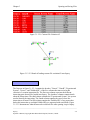
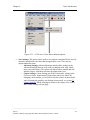
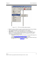
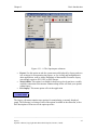
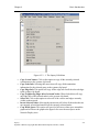
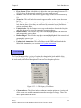
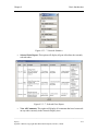
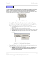
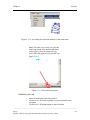
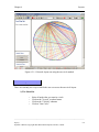
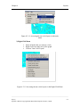
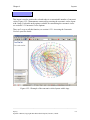
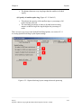
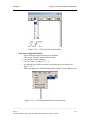
1
Osprey Network Visualization System
Reference Manual for Version 1.2.0
User Guide and Tutorial
Osprey Network Visualization System
Reference Manual for Version 1.2.0
Written by: Chris Stark, Bobby-Joe Breitkreutz
COPYRIGHT 2002
No part of this Guide may be reproduced, stored in a retrieval system or transmitted, in
any form or by any means, electronic, mechanical, photocopying, microfilming,
recording, or otherwise, without written permission from Mount Sinai Hospital, Toronto,
Canada.
For Technical Assistance
If you need help to resolve a problem, there are several ways to contact the Osprey team:
World Wide Web
http://biodata.mshri.on.ca/osprey/
E-mail
[email protected]
Copyright Notice
Copyright ©2002 Mount Sinai Hospital, Toronto, Canada. All Rights Reserved.
Warning: This system may be monitored by system or security personnel.
License Agreement for the Osprey Network Visualization System and all documentation
THIS AGREEMENT SETS OUT THE TERMS AND CONDITIONS FOR
DOWNLOADING, COPYING, INSTALLING, OR USING OSPREY NETWORK
VISUALIZATION SYSTEM SOFTWARE AND ASSOCIATED MATERIAL AND
DOCUMENTATION INCLUDING ANY MODIFIED VERSIONS OR UPDATES
(COLLECTIVELY “SOFTWARE”).
READ THE TERMS OF THIS AGREEMENT AND ANY PROVIDED
SUPPLEMENTAL LICENSE TERMS (COLLECTIVELY "AGREEMENT")
CAREFULLY BEFORE OPENING THE SOFTWARE PACKAGE. BY OPENING
THE SOFTWARE PACKAGE, YOU AGREE TO THE TERMS OF THIS
AGREEMENT AND THAT IT IS ENFORCEABLE LIKE ANY WRITTEN
NEGOTIATED AGREEMENT SIGNED BY YOU. INDICATE YOUR ACCEPTANCE
OF THESE TERMS BY SELECTING THE "ACCEPT" BUTTON AT THE END OF
THIS AGREEMENT. IF YOU DO NOT AGREE TO ALL OF THESE TERMS,
SELECT THE "DISAGREE" BUTTON AT THE END OF THIS AGREEMENT AND
THE SOFTWARE DOWNLOAD WILL NOT CONTINUE.
Restrictions
All downloads and use of the Osprey Network Visualization System are subject to the
following terms:
As long as you comply with the terms of this Agreement, you are granted a non-exclusive
license to install and use the Software on a single computer for educational, research, and
not-for-profit purposes, without fee. Except as expressly permitted in this Agreement,
you may not use, copy, decompile, reverse engineer, disassemble, modify, rent, lease,
loan, sublicense, distribute or create derivative works based upon the Software in whole
or part or transmit the Software over a network.
You shall not remove any copyright notices or other proprietary notices from the
Software.
Except as expressly stated herein this Agreement does not grant you any intellectual
property rights in the Software and all rights not expressly granted herein are reserved by
Mount Sinai Hospital.
The right to download, copy, install, use, and distribute this software and its
documentation by companies or other for profit organizations or in conjunction with for
profit activities, are not granted except by prior written arrangement of the copyright
holder. For commercial licensing opportunities contact [email protected] or visit
http://biodata.mshri.on.ca/osprey/servlet/CommercialRegistration/ for more details.
Termination
This Agreement and your license to use the Software will continue so long as you remain
in compliance with the terms and conditions of this Agreement. Your license will
terminate automatically without notice from Mount Sinai Hospital if you breach any of
your obligations hereunder. Upon termination, you shall cease using the Software and
shall destroy all copies of the Software (and associated materials and documentation) in
any form. All disclaimers of warranties and limitations of liability shall survive any
termination of this Agreement.
Disclaimers
IN NO EVENT SHALL MOUNT SINAI HOSPITAL BE LIABLE TO ANY PARTY
FOR DIRECT, INDIRECT, SPECIAL, INCIDENTAL, OR CONSEQUENTIAL
DAMAGES, INCLUDING LOST PROFITS, ARISING OUT OF THE USE OR
INABILITY TO USE THIS SOFTWARE AND ITS DOCUMENTATION, EVEN IF
MOUNT SINAI HOSPITAL HAS BEEN ADVISED OF THE POSSIBILITY OF SUCH
DAMAGE.
THE SOFTWARE AND ACCOMPANYING DOCUMENTATION, IF ANY,
PROVIDED HEREUNDER IS PROVIDED "AS IS". MOUNT SINAI HOSPITAL
SPECIFICALLY DISCLAIMS ANY IMPLIED WARRANTIES OF ANY KIND
INCLUDING BUT NOT LIMITED TO WARRANTIES OF MERCHANTABILITY,
NONFRINGEMENT, AND FITNESS FOR A PARTICULAR PURPOSE. MOUNT
SINAI HOSPITAL HAS NO OBLIGATION TO PROVIDE MAINTENANCE,
SUPPORT, UPDATES, ENHANCEMENTS, OR MODIFICATIONS. MOUNT SINAI
HOSPITAL DOES NOT WARRANT OR ASSUME RESPONSIBILITY FOR THE
ACCURACY OR COMPLETENESS OF ANY INFORMATION, TEXT, GRAPHICS,
LINKS, OR OTHER ITEMS CONTAINED WITHIN THE SOFTWARE.
Published research assisted by this software should cite:
Breitkreutz, BJ., Stark, C., Tyers M. "Osprey: A Network Visualization System."
Genome Biology 2003 4(3):R22
Table of Contents
1
General Information………………………….…………………………….. 1-1
1.1 About this Manual...…………………………………………………….
1.1.1 Convections Used in the Manual…………………………………
1.2 What is Osprey….………………………………………………………
1.2.1 The Main Features of Osprey…………………………………….
1.3 Copyright Notice………………………………………………………..
1.4 Contact Information……………………………………………………..
1.5 Osprey Licensing………………………………………………………..
1.6 Joining the Osprey Mailing List………………………………………...
2
1-2
1-2
1-3
1-3
1-4
1-6
1-6
1-6
Osprey Installation…………………………………………………………. 2-1
2.1 Obtaining Osprey.....…………………………………………………….
2.1.1 The Osprey Homepage…………………………………………...
2.1.2 Registering………………………………………………………..
2.1.3 Downloading……………………………………………………..
2.1.3.1 Downloading for Windows………………………………….
2.1.3.2 Downloading for Red Hat……………………………………
2.1.3.3 Downloading for Mac OS X…………………………………
2.2 Standard Installation Procedure for Microsoft Windows Systems (ME,
XP, 2000, 98, 95, NT)………………………………………………….
2.3 Standard Installation Procedure for Red Hat Linux Systems (versions
7.3 or Higher)…………………………………………………………...
2.4 Standard Installation Procedure for Mac OS X (versions 10.2 or
Higher)………………………………………………………………….
2.5 Post Installation…………………………………………………………
2.5.1 Running Osprey on Microsoft Windows Systems (ME, XP,
2000, 98, 95, NT)…………………………………………………
2.5.2 Running Osprey on Red Hat Linux Systems (versions 7.3 or
Higher)……………………………………………………………
2.5.3 Running Osprey on Mac OS X (versions 10.2 or Higher)……….
2.6 Common Installation Issues……………………………………………..
2.7 Uninstalling Osprey……………………………………………………..
2.7.1 Uninstalling Osprey on Microsoft Windows Systems (ME, XP,
2000, 98, 95, NT)…………………………………………………
2.7.2 Uninstalling Osprey on Red Hat Linux Systems (versions 7.3 or
Higher)……………………………………………………………
2.7.3 Uninstalling Osprey on Mac OS X (versions 10.2 or Higher)…...
2.8 Version Checking……………………………………………………….
2-1
2-1
2-2
2-7
2-11
2-12
2-14
2-15
2-22
2-32
2-40
2-40
2-41
2-41
2-43
2-43
2-43
2-46
2-46
2-48
______________________________________________________________________________________
Osprey
Operator’s Manual, Copyright 2002 Mount Sinai Hospital, Toronto, Canada
i
Table of Contents
3
4
Opening and Saving Files.………………………………………………….
3-1
3.1 Types of Files Opened by Osprey………………………………………
3.1.1 Osprey File……………………………………………………….
3.1.2 Custom File……………………………………………………….
3.1.2.1 Custom File Variation #1…………………………………….
3.1.2.2 Custom File Variation #2…………………………………….
3.1.2.3 Custom File Variation #3…………………………………….
3.1.2.4 Custom File Variation #4…………………………………….
3.1.3 Gene List………………………………………………………….
3.1.3.1 Gene List Variation #1……………………………………….
3.1.3.2 Gene List Variation #2……………………………………….
3.1.4 Opening Datasets…………………………………………………
3.1.4.1 Downloading new datasets…………………………………...
3.1.4.2 Adding personal datasets……………………………………..
3.1.5 Superimposing Datasets………………………………………….
3.2 Saving to Osprey Files ( .osp )………………………………………….
3.3 Exporting………………………………………………………………..
3.3.1 Image Types……………………………………………………...
3.3.1.1 JPEG………………………………………………………….
3.3.1.2 PNG…………………………………………………………..
3.3.1.3 SVG (Scalable Vector Graphics)……………………………..
3.3.2 Matrix…………………………………………………………….
3.3.3 How to Export……………………………………………………
3-1
3-1
3-1
3-2
3-3
3-4
3-5
3-7
3-7
3-8
3-9
3-10
3-12
3-13
3-14
3-16
3-16
3-16
3-16
3-17
3-17
3-17
Basic Introduction.………………………………………………………….
4-1
4.1 Osprey Layout…………………………………………………………..
4.2 Osprey Menus…………………………………………………………...
4.2.1 File Menu…………………………………………………………
4.2.2 Edit Menu………………………………………………………...
4.2.3 View Menu……………………………………………………….
4.2.4 Insert Menu……………………………………………………….
4.2.5 Format Menu……………………………………………………..
4.2.6 Filter Menu……………………………………………………….
4.2.7 Layout Menu……………………………………………………...
4.2.8 Help Menu………………………………………………………..
4.2.9 Database Menu…………………………………………………...
4.3 Networks………………………………………………………………...
4.3.1 Network Display Area……………………………………………
4.3.2 Manipulating the Network………………………………………..
4.3.2.1 Selecting Nodes………………………………………………
4.3.2.2 Selecting Edges………………………….……………………
4.3.2.3 Moving Individual Nodes…………………………………….
4.3.2.4 Selecting Multiple Nodes…………………………………….
4-1
4-2
4-3
4-7
4-9
4-14
4-14
4-17
4-18
4-21
4-22
4-23
4-24
4-25
4-25
4-27
4-28
4-28
______________________________________________________________________________________
Osprey
Operator’s Manual, Copyright 2002 Mount Sinai Hospital, Toronto, Canada
ii
Table of Contents
5
4.3.2.5 Moving Multiple Nodes………………………………………
4.3.2.6 Removing Nodes……………………………………………..
4.3.2.7 Removing Edges…………………………………..…………
4.3.2.8 Showing Loner Nodes………………………………………..
4.3.3 Network Display Area Command Menu…………………………
4.4 Gene/Edge Info Area……………………………………………………
4.4.1 Changing Screen Name…………………………………………..
4.4.2 Adding Comments………………………………………………..
4.4.3 Viewing Selected Node Report…………………………………..
4.4.4 Update Annotation………………………………………………..
4.4.5 Edge Info…………………………………………………………
4.5 Adding Interactions……………………………………………………..
4.5.1 From the Orf Info Area…………………………………………...
4.5.2 From the Network Display Area Command Menu and Insert
Menu……………………………………………………………...
4.5.2.1 Adding all interactions to selected vertices…………………..
4.5.2.2 Adding only interactions within Selected Vertices…………..
4.6 Colour Indices…………………………………………………………...
4.6.1 Go Process Index…………………………………………………
4.6.2 Experimental Systems Index……………………………………..
4.6.3 Sources Index…………………………………………………….
4.6.4 Saving Colour Indices……………………………………………
4.7 Multiple Organism Support……………………………………………..
4-29
4-29
4-31
4-33
4-35
4-36
4-37
4-39
4-42
4-44
4-45
4-45
4-46
Filters.………………………………………………………………………..
5-1
5.1 Network Filters………………………………………………………….
5.1.1 Accessing Network Filters………………………………………..
5.1.2 Using the Network filtering windows……………………………
5.1.2.1 Overview of the network filtering window…………………..
5.1.2.2 Filtering nodes out……………………………………………
5.1.2.3 Adding nodes back…………………………………………...
5.1.2.4 Grouping items……………………………………………….
5.1.3 Experimental Systems……………………………………………
5.1.4 Sources……………………………………………………………
5.1.5 GO Process……………………………………………………….
5.1.6 Turn Off Filters…………………………………………………...
5.2 Connectivity Filters……………………………………………………..
5.2.1 Accessing Connection Filters…………………………………….
5.2.2 Minimum…………………………………………………………
5.2.3 Iterative Minimum………………………………………………..
5-1
5-2
5-5
5-5
5-6
5-10
5-14
5-16
5-18
5-21
5-24
5-25
5-25
5-26
5-27
4-48
4-48
4-51
4-54
4-55
4-56
4-56
4-57
4-60
______________________________________________________________________________________
Osprey
Operator’s Manual, Copyright 2002 Mount Sinai Hospital, Toronto, Canada
iii
Table of Contents
5.2.4
5.2.5
6
7
Depth……………………………………………………………..
Turn Off Connectivity……………………………………………
5-27
5-28
Layouts.……………………………………………………………………...
6-1
6.1 Auto Relaxation…………………………………………………………
6.1.1 Accessing the auto relaxation from the main menu……………...
6.2 Circular Layouts………………………………………………………...
6.2.1 One Circle………………………………………………………...
6.2.1.1 Accessing the one circle layout………………………………
6.2.2 Concentric Circles………………………………………………..
6.2.2.1 Accessing the concentric circles layout………………………
6.2.3 Concentric Circles Options……………………………………….
6.2.3.1 Accessing the Concentric Circles Options…………………...
6.3 Dual Ring Layouts………………………………………………………
6.4 Spokes…………………………………………………………………...
6.4.1 Default Spokes……………………………………………………
6.4.1.1 Accessing the default spoke model…………………………..
6.4.2 Forced Spokes…………………………………………………….
6.4.2.1 Accessing the forced spoke model…………………………...
6.4.3 Spoke Options…………………………………………………….
6.4.3.1 Accessing the spoke options………………………………….
6.5 Global Layouts………………………………………………………….
6.5.1 Spoked Dual Ring………………………………………………...
6.5.1.1 Accessing Spoked Dual Ring Layout………………………...
6.5.2 Spoked Dual Ring Options……………………………………….
6.5.2.1 Accessing Spoked Dual Ring Layout Option settings………..
6.6 Functional Clustering…………………………………………………...
6.6.1 Accessing Functional Clustering options………………………...
6.6.2 GO Process Order………………………………………………...
6.6.3 Cluster Gap Size………………………………………………….
6.6.4 Turning Functional Clustering On/Off…………………………...
6.6.5 Degree of GO Process colouring…………………………………
6-1
6-1
6-3
6-3
6-4
6-6
6-7
6-8
6-10
6-11
6-13
6-14
6-15
6-16
6-17
6-18
6-20
6-21
6-21
6-22
6-23
6-25
6-26
6-27
6-27
6-31
6-33
6-34
Osprey Preferences and Customization.………………………………..…
7-1
7.1 Graph Colouring………………………………………………………...
7.1.1 Accessing Graph Colouring………………………………………
7.2 Drawing / Dragging Graph options……………………………………..
7.2.1 Accessing Drawing/Dragging graph options……………………..
7.3 Node Options……………………………………………………………
7.3.1 Choosing Method of Colouring Nodes …………………………..
7.3.2 User Defined Node Colours……………………………………...
7-1
7-2
7-3
7-4
7-7
7-7
7-9
______________________________________________________________________________________
Osprey
Operator’s Manual, Copyright 2002 Mount Sinai Hospital, Toronto, Canada
iv
Table of Contents
8
7.3.3 Colour Choosing Window………………………………………..
7.3.3.1 Swatches tab………………………………………………….
7.3.3.2 HSB tab……………………………………………………….
7.3.3.3 RGB tab………………………………………………………
7.3.4 Node Size…………………………………………………………
7.4 Edge Options……………………………………………………………
7.4.1 Choosing Method of Colouring Edges…………………………...
7.4.2 User Defined Edge Colours………………………………………
7.4.3 Edge Size…………………………………………………………
7.5 Arrow Head Options…………………………………………………….
7.5.1 User Defined Arrow Head Colour………………………………..
7.5.2 Arrow Head Size…………………………………………………
7.6 Label Options…………………………………………………………...
7.6.1 Label Size………………………………………………………...
7.6.2 Label Font………………………………………………………...
7.6.3 Label Style………………………………………………………..
7.6.4 Label Colour……………………………………………………...
7.6.5 Hiding Labels…………………………………………………….
7.7 Background Colour……………………………………………………...
7.7.1 Accessing Background Colour…………………………………...
7.8 Saving Preferences……………………………………………………...
7.8.1 Saving settings……………………………………………………
7.8.1.1 Saving Advanced Settings……………………………………
7.8.1.2 Saving Colour Settings……………………………………….
7.9 Proxy Settings…………………………………………………………...
7.10 Changing Databases…………………………………………………….
7.11 Memory Settings………………………………………………………...
7-11
7-11
7-12
7-13
7-14
7-16
7-16
7-19
7-20
7-21
7-22
7-23
7-25
7-25
7-27
7-28
7-29
7-30
7-31
7-31
7-34
7-34
7-35
7-35
7-36
7-37
7-43
The GRID (The General Repository of Interaction Datasets)………...…
8-1
8.1 Where to find The GRID……………………………………………….. 8-1
8.2 Osprey and The GRID………………………………………………….. 8-1
A Known Problems and Common Errors.………………………………...… A-1
A.1
A.2
A.3
A.4
A.5
What to do if you Encounter an Error…………………………………..
The Osprey Error Log…………………………………………………...
Reporting Errors to the Osprey Team…………………………………...
Known Problems………………………………………………………..
Common Errors…………………………………………………………
A.5.1 Unable to Install Osprey under a Windows 2000, NT, or XP…….
A.5.2 Unable to Add Interactions………………………………………..
A-1
A-1
A-2
A-2
A-3
A-3
A-3
______________________________________________________________________________________
Osprey
Operator’s Manual, Copyright 2002 Mount Sinai Hospital, Toronto, Canada
v
Table of Contents
B Credits…………………………….…………………………………..…...… B-1
B.1 The Osprey Team
B.2 The Osprey Contributors
B.3 The Osprey Supporters
B-1
B-1
B-2
C Future Updates and Obtaining Patches…...………………………..…...… C-1
D Osprey Change History…………………………………………………….. D-1
E Purchasing Osprey Licenses for Commercial Organizations…………… E-1
E.1 Commercial Applications……………………………………………. E-1
______________________________________________________________________________________
Osprey
Operator’s Manual, Copyright 2002 Mount Sinai Hospital, Toronto, Canada
vi
1. General Information
The Osprey Network Visualization System (Copyright ©2002 Mount Sinai Hospital) is a
tool for visualization and manipulation of complex interaction networks. Osprey builds
data-rich graphical representations that are color-coded for gene function and
experimental interaction data. Mouse-over functions allow rapid elaboration and
organization of network diagrams in a spoke model format. User-defined large-scale data
sets can be readily combined with Osprey for comparison of different methods. The
Osprey Network Visualization System is a copyright of the Samuel Lunenfeld Research
Institute at Mount Sinai Hospital in Toronto, Ontario, Canada.
For all of the latest information about Osprey, including latest patches and updates,
please visit the Osprey web site ( http://biodata.mshri.on.ca/osprey ).
The following list describes some sections of particular interest in this manual:
•
•
•
•
•
•
•
•
For information about the developers and team behind Osprey, see appendix B.
Credits
For information about joining the Osprey mailing list, see section 1.6 Joining the
Osprey Mailing List
For installation instructions, see section 2. Osprey Installation
For a listing of basic Osprey layouts and descriptions, see section 4. Basic
Introduction
For a history of new features and bug fixes, see appendix D. Osprey Change
History
For a list of currently known bugs and misfeatures, see appendix A. Known
Problems and Common Errors
For future Osprey plans, see appendix C. Future Updates and Obtaining Patches
For more information about The GRID, see section 8. The GRID ( The General
Repository of Interaction Datasets )
Important:
Reports of any errors (often called bugs), as well as questions and comments, should be
sent to [email protected]. For more information on contacting us, please see
section 1.4 Contact Information
______________________________________________________________________________________
Osprey
Operator’s Manual, Copyright 2002 Mount Sinai Hospital, Toronto, Canada
1-1
Chapter 1
General Information
1.1 About this Manual
This is the Osprey Network Visualization System manual. Being a reference manual, it
does not provide any general information on the actual development involved in the
product. No documentation of source code or tools is provided within as Osprey is under
constant development, this manual is also updated frequently. The most recent version of
the manual is available at (http://biodata.mshri.on.ca/osprey) in various formats.
If you have any suggestions concerning additions or corrections to this manual, please
send them to the documentation team at [email protected].
This manual was initially written by Bobby-Joe Breitkreutz, Chris Stark, and Hosam
Abdulrrazek. It is currently maintained by the Osprey development team at Mount Sinai
Hospital. For other contributors, please see section B. Credits,
The copyright (© 2002) to this manual is owned by Mount Sinai Hospital in Toronto,
Ontario. See section 1.3 Copyright Notice.
This manual is best viewed with Microsoft Internet Explorer version 6.0+ or
Netscape/Mozilla version 1.1+
1.1.1 Conventions used in this manual
This manual uses the following Typographical Conventions:
Links
Represents Links either to external pages, or to other pages
inside this reference manual
HEADINGS
Denotes the start of a new section or subsection in this
manual
______________________________________________________________________________________
Osprey
Operator’s Manual, Copyright 2002 Mount Sinai Hospital, Toronto, Canada
1-2
Chapter 1
General Information
1.2 What is Osprey
Osprey is a tool for graphically representing biological interactions. It can be used in one
of two ways
1. As a freely distributed standalone version available at
(http://biodata.mshri.on.ca/osprey)
2. As an add-on interaction visualization system for use with online interaction
databases (see section 1.5 Osprey Licensing for more details)
For all of the latest information concerning Osprey, please visit the Osprey web page at
(http://biodata.mshri.on.ca/osprey)
1.2.1 The Main Features of Osprey
The following list describes some of the important characteristics of the Osprey Network
Visualization System:
•
•
•
•
•
•
Portability (cross platform availability)
o Osprey is available on almost all Platforms that support the latest Java
Plugin
Tools for Biological Analysis
o Osprey provides many features such as network filters, connectivity
filters, advanced layouts, and dataset superimposing which are extremely
useful to biologists who are interested in analyzing their data
Powerful Support Database
o Integrated with Osprey is a powerful database of interactions and
annotation, see section 8. The GRID (The General Repository of
Interaction Datasets).
Ease of use
o Osprey provides an extremely user friendly interface for working with
interaction data
Online Database Add-on Ability
o Osprey can be incorporated as a standard visualization tool with online
databases such as The GRID (http://biodata.mshri.on.ca/grid)
Support for figures
o Osprey networks can be saved in SVG, PNG and JPG format so they can
be used with image programs
______________________________________________________________________________________
Osprey
Operator’s Manual, Copyright 2002 Mount Sinai Hospital, Toronto, Canada
1-3
Chapter 1
General Information
1.3 Copyright Notice
Copyright ©2002 Mount Sinai Hospital, Toronto, Canada. All Rights Reserved.
Warning: This system may be monitored by system or security personnel.
License Agreement for the Osprey Network Visualization System and all documentation
THIS AGREEMENT SETS OUT THE TERMS AND CONDITIONS FOR
DOWNLOADING, COPYING, INSTALLING, OR USING OSPREY NETWORK
VISUALIZATION SYSTEM SOFTWARE AND ASSOCIATED MATERIAL AND
DOCUMENTATION INCLUDING ANY MODIFIED VERSIONS OR UPDATES
(COLLECTIVELY “SOFTWARE”).
READ THE TERMS OF THIS AGREEMENT AND ANY PROVIDED
SUPPLEMENTAL LICENSE TERMS (COLLECTIVELY "AGREEMENT")
CAREFULLY BEFORE OPENING THE SOFTWARE PACKAGE. BY OPENING
THE SOFTWARE PACKAGE, YOU AGREE TO THE TERMS OF THIS
AGREEMENT AND THAT IT IS ENFORCEABLE LIKE ANY WRITTEN
NEGOTIATED AGREEMENT SIGNED BY YOU. INDICATE YOUR ACCEPTANCE
OF THESE TERMS BY SELECTING THE "ACCEPT" BUTTON AT THE END OF
THIS AGREEMENT. IF YOU DO NOT AGREE TO ALL OF THESE TERMS,
SELECT THE "DISAGREE" BUTTON AT THE END OF THIS AGREEMENT AND
THE SOFTWARE DOWNLOAD WILL NOT CONTINUE.
Restrictions
All downloads and use of the Osprey Network Visualization System are subject to the
following terms:
As long as you comply with the terms of this Agreement, you are granted a non-exclusive
license to install and use the Software on a single computer for educational, research, and
not-for-profit purposes, without fee. Except as expressly permitted in this Agreement,
you may not use, copy, decompile, reverse engineer, disassemble, modify, rent, lease,
loan, sublicense, distribute or create derivative works based upon the Software in whole
or part or transmit the Software over a network.
You shall not remove any copyright notices or other proprietary notices from the
Software.
Except as expressly stated herein this Agreement does not grant you any intellectual
property rights in the Software and all rights not expressly granted herein are reserved by
Mount Sinai Hospital.
______________________________________________________________________________________
Osprey
Operator’s Manual, Copyright 2002 Mount Sinai Hospital, Toronto, Canada
1-4
Chapter 1
General Information
The right to download, copy, install, use, and distribute this software and its
documentation by companies or other for profit organizations or in conjunction with for
profit activities, are not granted except by prior written arrangement of the copyright
holder. For commercial licensing opportunities contact [email protected] or visit
http://biodata.mshri.on.ca/osprey/servlet/CommercialRegistration/ for more details.
Termination
This Agreement and your license to use the Software will continue so long as you remain
in compliance with the terms and conditions of this Agreement. Your license will
terminate automatically without notice from Mount Sinai Hospital if you breach any of
your obligations hereunder. Upon termination, you shall cease using the Software and
shall destroy all copies of the Software (and associated materials and documentation) in
any form. All disclaimers of warranties and limitations of liability shall survive any
termination of this Agreement.
Disclaimers
IN NO EVENT SHALL MOUNT SINAI HOSPITAL BE LIABLE TO ANY PARTY
FOR DIRECT, INDIRECT, SPECIAL, INCIDENTAL, OR CONSEQUENTIAL
DAMAGES, INCLUDING LOST PROFITS, ARISING OUT OF THE USE OR
INABILITY TO USE THIS SOFTWARE AND ITS DOCUMENTATION, EVEN IF
MOUNT SINAI HOSPITAL HAS BEEN ADVISED OF THE POSSIBILITY OF SUCH
DAMAGE.
THE SOFTWARE AND ACCOMPANYING DOCUMENTATION, IF ANY,
PROVIDED HEREUNDER IS PROVIDED "AS IS". MOUNT SINAI HOSPITAL
SPECIFICALLY DISCLAIMS ANY IMPLIED WARRANTIES OF ANY KIND
INCLUDING BUT NOT LIMITED TO WARRANTIES OF MERCHANTABILITY,
NONFRINGEMENT, AND FITNESS FOR A PARTICULAR PURPOSE. MOUNT
SINAI HOSPITAL HAS NO OBLIGATION TO PROVIDE MAINTENANCE,
SUPPORT, UPDATES, ENHANCEMENTS, OR MODIFICATIONS. MOUNT SINAI
HOSPITAL DOES NOT WARRANT OR ASSUME RESPONSIBILITY FOR THE
ACCURACY OR COMPLETENESS OF ANY INFORMATION, TEXT, GRAPHICS,
LINKS, OR OTHER ITEMS CONTAINED WITHIN THE SOFTWARE.
Published research assisted by this software should cite:
Breitkreutz, BJ., Stark, C., Tyers M. "Osprey: A Network Visualization System."
Genome Biology 2003 4(3):R22
______________________________________________________________________________________
Osprey
Operator’s Manual, Copyright 2002 Mount Sinai Hospital, Toronto, Canada
1-5
Chapter 1
General Information
1.4 Contact Information
For commercial licensing opportunities, suggestions, corrections, bug reports, more
information or for joining our mailing list, contact:
The Osprey Administrator
E-mail: [email protected]
1.5 Osprey Licensing
Please see section E. Purchasing Osprey Licenses for Commercial
Organizations for full details of Osprey licensing policy.
1.6 Joining the Osprey Mailing List
To be kept up to date on all the latest bug fixes, version releases, and other information
about the Osprey Network Visualization System, please subscribe to the Osprey mailing
list by sending an email to:
The Osprey Administrator
E-mail: [email protected]
Or visit the Osprey web site at http://biodata.mshri.on.ca/Osprey
______________________________________________________________________________________
Osprey
Operator’s Manual, Copyright 2002 Mount Sinai Hospital, Toronto, Canada
1-6
2. Osprey Installation
This section describes how to obtain and install Osprey on supported operating systems.
The following lists the operating systems in which Osprey can be installed:
•
•
•
Microsoft Windows operating systems ( 95, 98, NT, ME, 2000, XP )
Red Hat Linux systems ( ver. 7.3 or higher )
Mac OS X ( ver. 10.2 or higher )
If you are currently not running one of these operating systems, Osprey will not work
with your computer. We are looking into solutions for other systems, such as Solaris, so
if your system is not currently supported, please be sure to check back as we continue to
make updates.
2.1 Obtaining Osprey
Before proceeding with installation, you must first obtain a copy of the Osprey installer
that is appropriate for your system. The following subsections outline where and how to
get the installer. To obtain Osprey, you must be on a computer that is connected to the
Internet.
2.1.1 The Osprey Homepage
To obtain a copy of Osprey, you must first visit the Osprey homepage located at [
http://biodata.mshri.on.ca/osprey ]. If you are unable to access the Internet in order to
visit the Osprey homepage, you may request a CD copy of Osprey by contacting us.( see
section 1.4 Contact Information ).
______________________________________________________________________________________
Osprey
Operator’s Manual, Copyright 2002 Mount Sinai Hospital, Toronto, Canada
2-1
Chapter 2
Osprey Installation
Figure 2.1.1 - 1: The main page of the Osprey homepage
2.1.2 Registering
In order to download Osprey, you must first register and obtain a password. Registration
is easy, and completely free. Simply click on the Download link of the operating system
you are using to begin the process.
______________________________________________________________________________________
Osprey
Operator’s Manual, Copyright 2002 Mount Sinai Hospital, Toronto, Canada
2-2
Chapter 2
Osprey Installation
Figure 2.1.2 - 1: The location of the Download link on the Osprey homepage
There are two versions of Osprey available for download. The academic version and our
30-Day trial version (see figure 2.1.2 - 1b). You must download the 30-Day trial version
if you fall into any of the following 3 categories:
•
•
•
If you plan to distribute Osprey with any other application
If your organization is non-academic or for-profit
If you wish to support further Osprey development
The 30-Day trial version is a fully functioning version of Osprey for testing use by
Commercial organizations. After 30-Days, you will need to purchase an Osprey license
(http://biodata.mshri.on.ca/osprey/servlet/CommercialRegistration) to continue using
Osprey. All academic users are free to download our fully functioning and free Osprey
academic version for all major platforms.
______________________________________________________________________________________
Osprey
Operator’s Manual, Copyright 2002 Mount Sinai Hospital, Toronto, Canada
2-3
Chapter 2
Osprey Installation
Figure 2.1.2 - 1b: The Osprey download page, with all versions both Academic and
Commercial available for download
Choose the version that is appropriate for you (academic or commercial) and the platform
you will be running Osprey on (Mac OS X, Windows, or Linux), by clicking the link
associated with that version. This will take you to the Osprey download login page. If
you already have an account, you can simply login here to proceed with the download. If
you do not have an account simply click the large red button entitled "CLICK HERE TO
REGISTER" to proceed with Osprey download registration.
______________________________________________________________________________________
Osprey
Operator’s Manual, Copyright 2002 Mount Sinai Hospital, Toronto, Canada
2-4
Chapter 2
Osprey Installation
Figure 2.1.2 - 2: The Download Login page with the registration link shown
Fill in all of the fields and click the register button to register with Osprey. Please ensure
that you have used an email address that is valid, because all Osprey correspondence,
including obtaining passwords, will be done via this account.
______________________________________________________________________________________
Osprey
Operator’s Manual, Copyright 2002 Mount Sinai Hospital, Toronto, Canada
2-5
Chapter 2
Osprey Installation
Figure 2.1.2 - 3: An Osprey registration form
______________________________________________________________________________________
Osprey
Operator’s Manual, Copyright 2002 Mount Sinai Hospital, Toronto, Canada
2-6
Chapter 2
Osprey Installation
Figure 2.1.2 - 4: The resulting page after a successful registration
2.1.3 Downloading
Once you have registered, and you have received an email from Osprey containing your
account name and password, you are now ready to download Osprey. If for some reason,
you have successfully registered, but did not receive an email containing you password,
please contact us ( see section 1.4 Contact Information ). Before downloading, you must
first login to the downloads area using your newly acquired Osprey password.
______________________________________________________________________________________
Osprey
Operator’s Manual, Copyright 2002 Mount Sinai Hospital, Toronto, Canada
2-7
Chapter 2
Osprey Installation
Figure 2.1.3 - 1: The Osprey download login page
After login you will be prompted with the copyright notice that you must agree with
before proceeding to the downloads page. See section 1.3 Copyright Notice for more
details.
______________________________________________________________________________________
Osprey
Operator’s Manual, Copyright 2002 Mount Sinai Hospital, Toronto, Canada
2-8
Chapter 2
Osprey Installation
Figure 2.1.3 - 2: The Copyright Page
After agreeing to the copyright notice you will be presented with the ability to download
Osprey for the operating system you selected at the begriming of the installation
procedure.
______________________________________________________________________________________
Osprey
Operator’s Manual, Copyright 2002 Mount Sinai Hospital, Toronto, Canada
2-9
Chapter 2
Osprey Installation
Figure 2.1.3 - 3: The downloads page
______________________________________________________________________________________
Osprey
Operator’s Manual, Copyright 2002 Mount Sinai Hospital, Toronto, Canada
2-10
Chapter 2
Osprey Installation
2.1.3.1 Downloading for Windows
Figure 2.1.3.1 - 1: The Windows Osprey Download Page
There are three major sections to the download page for windows. Each of these is
necessary for downloading the Osprey Network Visualization System. The following is a
listing of the three sections shown in figure 2.1.3.1 - 1:
•
•
Section 1: This section contains your operating system specific download of
Osprey. Click on the link to download the osprey installer
Section 2: This section contains links for downloading instructions for installing
Osprey. You can download the installation instructions in the following format
o Adobe PDF (Portable Document Format): This is a file format that has
captured all the elements of a printed document as an electronic image that
you can view, navigate, print, or forward to someone else. PDF files are
created using Adobe Acrobat, Acrobat Capture, or similar products. To
______________________________________________________________________________________
Osprey
Operator’s Manual, Copyright 2002 Mount Sinai Hospital, Toronto, Canada
2-11
Chapter 2
•
Osprey Installation
view and use the files, you need the free Acrobat Reader, which you can
easily download.
o Text File (.txt): This format provides the installation documentation in a
plain text format that can easily be viewed in applications such as Word,
Wordpad, or Notepad. This format is limited in that it does not support the
use of screen shots.
o HTML: This format provides the installation documentation in a properly
formatted HTML web page. You must have a web browser available to
view this document. ( i.e. Netscape, Internet Explorer, Mozilla, etc )
Section 3: These are the system requirements for Osprey. Please be sure to read
these carefully before downloading and installing Osprey. On the left hand side,
are the minimum requirements. Any computer running with requirements less
than these, should not attempt to install Osprey. On the right hand side, are the
recommended requirements. For maximum performance, we highly recommend
using a computer that maintains these requirements.
2.1.3.2 Downloading for Red Hat
______________________________________________________________________________________
Osprey
Operator’s Manual, Copyright 2002 Mount Sinai Hospital, Toronto, Canada
2-12
Chapter 2
Osprey Installation
Figure 2.1.3.2 - 1: The Linux Osprey Download Page
There are three major sections to the download page for Linux. Each of these is necessary
for downloading the Osprey Network Visualization System. The following is a listing of
the three sections shown in figure 2.1.3.1 - 1:
•
•
•
Section 1: This section contains your operating system specific download of
Osprey. Click on the link to download the Osprey installer
Section 2: This section contains links for downloading instructions for installing
Osprey. You can download the installation instructions in the following format
o Adobe PDF (Portable Document Format): This is a file format that has
captured all the elements of a printed document as an electronic image that
you can view, navigate, print, or forward to someone else. PDF files are
created using Adobe Acrobat, Acrobat Capture, or similar products. To
view and use the files, you need the free Acrobat Reader, which you can
easily download.
o Text File (.txt): This format provides the installation documentation in a
plain text format that can easily be viewed in applications such as GEdit,
XEmacs/Emacs, NEdit, VI, or Pico. This format is limited in that it does
not support the use of screen shots.
o HTML: This format provides the installation documentation in a properly
formatted HTML web page. You must have a web browser available to
view this document. ( i.e. Netscape, Mozilla, Konqueror, Opera, Galeon,
etc )
Section 3: These are the system requirements for Osprey. Please be sure to read
these carefully before downloading and installing Osprey. On the left hand side,
are the minimum requirements. Any computer running with requirements less
than these, should not attempt to install Osprey. On the right hand side, are the
recommended requirements. For maximum performance, we highly recommend
using a computer that maintains these requirements.
______________________________________________________________________________________
Osprey
Operator’s Manual, Copyright 2002 Mount Sinai Hospital, Toronto, Canada
2-13
Chapter 2
Osprey Installation
2.1.3.3 Downloading for Mac OS X
Figure 2.1.3.3 - 1: The Mac OS X Osprey Download Page
There are three major sections to the download page for Mac OS X. Each of these is
necessary for downloading the Osprey Network Visualization System. The following is a
listing of the three sections shown in figure 2.1.3.3 - 1:
•
•
Section 1: This section contains your operating system specific download of
Osprey. Click on the link to download the Osprey installer
Section 2: This section contains links for downloading instructions for installing
Osprey. You can download the installation instructions in the following format
o Adobe PDF (Portable Document Format): This is a file format that has
captured all the elements of a printed document as an electronic image that
you can view, navigate, print, or forward to someone else. PDF files are
created using Adobe Acrobat, Acrobat Capture, or similar products. To
______________________________________________________________________________________
Osprey
Operator’s Manual, Copyright 2002 Mount Sinai Hospital, Toronto, Canada
2-14
Chapter 2
•
Osprey Installation
view and use the files, you need the free Acrobat Reader, which you can
easily download.
o Text File (.txt): This format provides the installation documentation in a
plain text format that can easily be viewed in applications such as GEdit,
XEmacs/Emacs, NEdit, VI, or Pico. This format is limited in that it does
not support the use of screenshots.
o HTML: This format provides the installation documentation in a properly
formatted HTML web page. You must have a web browser available to
view this document. ( i.e. Netscape, Mozilla, Konqueror, Opera, Galeon,
etc )
Section 3: These are the system requirements for Osprey. Please be sure to read
these carefully before downloading and installing Osprey. On the left hand side,
are the minimum requirements. Any computer running with requirements less
than these, should not attempt to install Osprey. On the right hand side, are the
recommended requirements. For maximum performance, we highly recommend
using a computer that maintains these requirements.
2.2 Standard Installation Procedure for Microsoft
Windows Systems ( ME, XP, 2000, 98, 95, NT )
In order to proceed with the Osprey installation for Windows, you must first download a
copy of Osprey. If you have not yet obtained a copy, see section 2.1 Obtaining Osprey for
more details. Once you have a copy of the Osprey installer ( osprey.exe ) you are ready to
continue.
The Osprey installation is very simple and easy. Installation is completely free, and will
take less than 5 minutes to complete. To proceed with installation, follow these steps:
1 ) Before installation you must extract, using WinZip (http://www.winzip.com/), the
executable from the "osprey.zip" file obtained after downloading Osprey. To begin the
installation, start by double-clicking the Osprey Installer ( osprey.exe ) and wait while
Osprey initializes some packages required for installation.
Figure 2.2 - 1: The Osprey Installer Icon
______________________________________________________________________________________
Osprey
Operator’s Manual, Copyright 2002 Mount Sinai Hospital, Toronto, Canada
2-15
Chapter 2
Osprey Installation
Figure 2.2 - 2: Osprey initializing packages before proceeding with installation
2) Once the Osprey installer has launched, you will be asked a series of questions about
your installation. Firstly, you are presented with an introduction to the install procedure.
Please read this carefully, and click "NEXT" to proceed.
Figure 2.2 - 3: Osprey installation introduction
______________________________________________________________________________________
Osprey
Operator’s Manual, Copyright 2002 Mount Sinai Hospital, Toronto, Canada
2-16
Chapter 2
Osprey Installation
3) Next, you will be presented with the Osprey Network Visualization System User
Agreement. Please read this carefully. By clicking "NEXT" you will agree to these terms
and conditions. If you do not agree to the terms and conditions, simply click "CANCEL"
at any time to abort the Osprey installation. If you agree, click the "NEXT" button to
continue.
Figure 2.2 - 4: Osprey Network Visualization System User Agreement
4) On the next screen, you will be asked about the installation folder for Osprey. By
default, Osprey uses C:\Program Files\osprey_1.0.0 as an installation directory. If you
would like to install in a different directory, select the new folder from this page. If you
are happy with the default installation folder, click "NEXT" to continue.
______________________________________________________________________________________
Osprey
Operator’s Manual, Copyright 2002 Mount Sinai Hospital, Toronto, Canada
2-17
Chapter 2
Osprey Installation
Figure 2.2 - 5: The Osprey Installation Choose Install Folder page
5) On the following screen, you will be presented with several options for installing
Osprey shortcuts. By defaults, Osprey will install shortcuts into the start menu ( program
group ) for you to access. If you would rather have the shortcuts installed elsewhere, you
can customize these options to suit your preferences. When you have made your shortcut
choice, click "NEXT" to continue.
______________________________________________________________________________________
Osprey
Operator’s Manual, Copyright 2002 Mount Sinai Hospital, Toronto, Canada
2-18
Chapter 2
Osprey Installation
Figure 2.2 - 6: Osprey Installation Choose Shortcut Folder page
6) The next page will outline the options you have selected in a pre-installation summary.
Please review the information, and ensure that everything is correct, and click "NEXT" to
continue.
______________________________________________________________________________________
Osprey
Operator’s Manual, Copyright 2002 Mount Sinai Hospital, Toronto, Canada
2-19
Chapter 2
Osprey Installation
Figure 2.2 - 7: Osprey Pre-Installation Summary
7) The Osprey install will now copy all of the files needed to run Osprey. This process
will take only a few minutes to run.
______________________________________________________________________________________
Osprey
Operator’s Manual, Copyright 2002 Mount Sinai Hospital, Toronto, Canada
2-20
Chapter 2
Osprey Installation
Figure 2.2 - 8: Osprey install progress copying files to your computer
8) Now the Osprey installation is complete. Click on the "DONE" button to finish the
install and close the Osprey installer.
______________________________________________________________________________________
Osprey
Operator’s Manual, Copyright 2002 Mount Sinai Hospital, Toronto, Canada
2-21
Chapter 2
Osprey Installation
Figure 2.2 - 9: Osprey Install Complete
2.3 Standard Installation Procedure for Red Hat Linux
Systems ( versions 7.3 or Higher )
In order to proceed with the Osprey installation for Linux, you must first download a
copy of Osprey. If you have not yet obtained a copy, see section 2.1 Obtaining Osprey for
more details. Once you have a copy of the Osprey installer ( osprey.tar.gz ) you are ready
to continue.
The Osprey installation is very simple and easy. Installation is completely free. To
proceed with installation, follow these steps:
1) Once you have downloaded Osprey to your local file system, you will have a file
called osprey.tar.gz. This is the compressed file containing the Osprey installer. You will
need to extract it before proceeding, which we will cover in the next few steps.
______________________________________________________________________________________
Osprey
Operator’s Manual, Copyright 2002 Mount Sinai Hospital, Toronto, Canada
2-22
Chapter 2
Osprey Installation
Figure 2.3 - 1: Command Line with the Osprey gzip'd file showing
2) To extract Osprey, first gunzip the file by executing the command "gunzip
osprey.tar.gz" and then untar the file by executing the command "tar -xvf osprey.tar"
(see figure 2.3-2)
______________________________________________________________________________________
Osprey
Operator’s Manual, Copyright 2002 Mount Sinai Hospital, Toronto, Canada
2-23
Chapter 2
Osprey Installation
Figure 2.3 - 2: Extracting the Osprey installer and installation manuals from the
compressed Osprey file
3) In order to execute the Osprey installer, you will have to set its permissions. To do
this, type "chmod 777 osprey_1_0_0.bin" at the command prompt (see figure 2.3-3)
Figure 2.3 - 3: Modifying the permissions of the Osprey.bin file to allow it to be executed
4) Once you have modified the permissions on the file, you can now execute the osprey
installer by typing: "./osprey_1_0_0.bin" at the command prompt
______________________________________________________________________________________
Osprey
Operator’s Manual, Copyright 2002 Mount Sinai Hospital, Toronto, Canada
2-24
Chapter 2
Osprey Installation
Figure 2.3 - 4: Osprey Installation File, and the command line option to run it
5) The Osprey installer will now launch, and the installation application will initialize
Figure 2.3 - 5: The Osprey installer initialization
______________________________________________________________________________________
Osprey
Operator’s Manual, Copyright 2002 Mount Sinai Hospital, Toronto, Canada
2-25
Chapter 2
Osprey Installation
6) Once the Osprey installer has launched, you will be asked a series of questions about
your installation. Firstly, you are presented with an introduction to the install procedure
(fig 2.3-6) Please read this carefully, and click "NEXT" to proceed.
Figure 2.3 - 6: The Osprey Installer Introduction
7) Next, you will be presented with the Osprey Network Visualization System User
Agreement. Please read this carefully. By clicking "NEXT" you will agree to these terms
and conditions. If you do not agree to the terms and conditions, simply click "CANCEL"
at any time to abort the osprey installation. If you agree, click the "NEXT" button to
continue.
______________________________________________________________________________________
Osprey
Operator’s Manual, Copyright 2002 Mount Sinai Hospital, Toronto, Canada
2-26
Chapter 2
Osprey Installation
Figure 2.3 - 7: Osprey Network Visualization System User Agreement
8) On the next screen, you will be asked about the installation folder for Osprey. By
default, Osprey uses /$home/Osprey as an installation directory. If you would like to
install in a different directory, select the new directory from this page. If you are happy
with the default installation folder, click "NEXT" to continue.
______________________________________________________________________________________
Osprey
Operator’s Manual, Copyright 2002 Mount Sinai Hospital, Toronto, Canada
2-27
Chapter 2
Osprey Installation
Figure 2.3 - 8: The Osprey Installation Choose Install Folder page
9) On the following screen, you will be presented with several options for installing
Osprey shortcuts. By defaults, Osprey will install shortcuts into your home folder for you
to access. If you would rather have the shortcuts installed elsewhere, such as /usr/bin, you
can customize these options to suit your preferences. When you have made your shortcut
choice, click "NEXT" to continue.
______________________________________________________________________________________
Osprey
Operator’s Manual, Copyright 2002 Mount Sinai Hospital, Toronto, Canada
2-28
Chapter 2
Osprey Installation
Figure 2.3 - 9: Osprey Installation Choose Shortcut Folder page
10) The next page will outline the options you have selected in a pre-installation
summary. Please review the information, and ensure that everything is correct, and click
"NEXT" to continue.
______________________________________________________________________________________
Osprey
Operator’s Manual, Copyright 2002 Mount Sinai Hospital, Toronto, Canada
2-29
Chapter 2
Osprey Installation
Figure 2.3 - 10: Osprey Pre-Installation Summary
11) The Osprey install will now copy all of the files needed to run Osprey. This process
will take only a few minutes to run.
______________________________________________________________________________________
Osprey
Operator’s Manual, Copyright 2002 Mount Sinai Hospital, Toronto, Canada
2-30
Chapter 2
Osprey Installation
Figure 2.3 - 11: Osprey install progress copying files to your computer
12) Now the Osprey installation is complete. Click on the "DONE" button to finish the
install and close the Osprey installer.
______________________________________________________________________________________
Osprey
Operator’s Manual, Copyright 2002 Mount Sinai Hospital, Toronto, Canada
2-31
Chapter 2
Osprey Installation
Figure 2.3 - 12: Osprey Install Complete
2.4 Standard Installation Procedure for Mac OS X (
versions 10.2 or Higher )
In order to proceed with the Osprey installation for Mac OS X, you must first download a
copy of Osprey and have java 1.4.1 working. Please run the software update to check if
you need to install the latest java for your Mac. If you have not yet obtained a copy, see
section 2.1 Obtaining Osprey for more details. Once you have a copy of the Osprey zip
file ( osprey.zip ) you are ready to continue.
The Osprey installation is very simple and easy. Installation is completely free. To
proceed with installation, follow these steps:
1 ) To begin the installation, start by executing the osprey.zip file, see figure 1, and wait
while Stuffit unzips the Osprey installer program, see figure 2, to continue execute this
file. Note you will need to have already installed stuffit onto your computer, see
http://www.stuffit.com/expander/ for more info.
______________________________________________________________________________________
Osprey
Operator’s Manual, Copyright 2002 Mount Sinai Hospital, Toronto, Canada
2-32
Chapter 2
Osprey Installation
Figure 1: The Osprey.zip Icon
Figure 2: Stuffit unzips the osprey installer program
2) Once the osprey installer has launched, you will be asked a series of questions about
your installation. Firstly, you are presented with an introduction to the install procedure,
see figure 3. Please read this carefully, and click "NEXT" to proceed.
______________________________________________________________________________________
Osprey
Operator’s Manual, Copyright 2002 Mount Sinai Hospital, Toronto, Canada
2-33
Chapter 2
Osprey Installation
Figure 3: Osprey installation introduction
3) Next, you will be presented with the Osprey Network Visualization System User
Agreement, see figure 4. Please read this carefully. By clicking "NEXT" you will agree to
these terms and conditions. If you do not agree to the terms and conditions, simply click
"CANCEL" at any time to abort the osprey installation. If you agree, click the "NEXT"
button to continue.
______________________________________________________________________________________
Osprey
Operator’s Manual, Copyright 2002 Mount Sinai Hospital, Toronto, Canada
2-34
Chapter 2
Osprey Installation
Figure 4: Osprey Network Visualization System User Agreement
4) On the next screen, you will be asked about the installation folder for Osprey, see
figure 5. By default, this would be located on the disk inside "osprey_1.0.0" in the folder
"Applications" as an installation directory. If you would like to install in a different
directory, select the new folder from this page. If you are happy with the default
installation folder, click "NEXT" to continue.
______________________________________________________________________________________
Osprey
Operator’s Manual, Copyright 2002 Mount Sinai Hospital, Toronto, Canada
2-35
Chapter 2
Osprey Installation
Figure 5: The Osprey Installation Choose Install Folder page
5) On the following screen, you will be presented with several options for installing
osprey shortcuts, see figure 6. By default, Osprey will install shortcuts on the desktop for
you to access. If you would rather have the shortcuts installed elsewhere, you can
customize these options to suit your preferences. When you have made your shortcut
choice, click "NEXT" to continue.
______________________________________________________________________________________
Osprey
Operator’s Manual, Copyright 2002 Mount Sinai Hospital, Toronto, Canada
2-36
Chapter 2
Osprey Installation
Figure 6: Osprey Installation Choose Shortcut Folder page
6) The next page will outline the options you have selected in a pre-installation summary,
see figure 7. Please review the information, and ensure that everything is correct, and
click "NEXT" to continue.
______________________________________________________________________________________
Osprey
Operator’s Manual, Copyright 2002 Mount Sinai Hospital, Toronto, Canada
2-37
Chapter 2
Osprey Installation
Figure 7: Osprey Pre-Installation Summary
7) The Osprey install will now copy all of the files needed to run Osprey, see figure 8.
______________________________________________________________________________________
Osprey
Operator’s Manual, Copyright 2002 Mount Sinai Hospital, Toronto, Canada
2-38
Chapter 2
Osprey Installation
Figure 8: Osprey install progress copying files to your computer
8) Now the Osprey installation is complete, see figure 9. Click on the "DONE" button to
finish the install and close the Osprey installer.
______________________________________________________________________________________
Osprey
Operator’s Manual, Copyright 2002 Mount Sinai Hospital, Toronto, Canada
2-39
Chapter 2
Osprey Installation
Figure 9: Osprey Install Complete
2.5 Post Installation
This section assumes that you have previously installed Osprey on your computer. If you
have not installed Osprey, see section 2.2 Standard Installation Procedure for Microsoft
Windows Systems ( ME, XP, 2000, 98, 95, NT ) or section 2.3 Standard Installation
Procedure for Red Hat Linux Systems ( versions 7.3 or Higher ) or section 2.4 Standard
Installation Procedure for Mac OS X ( versions 10.2 or Higher ) for installation
procedures.
2.5.1 Running Osprey on Microsoft Windows Systems ( ME, XP, 2000, 98, 95, NT )
Once Osprey has been installed on your computer, you can now start the application by
clicking on the Osprey shortcut. If you used the default install options this shortcut will
exist in your start menu in Windows, see figure 2.5-1.
______________________________________________________________________________________
Osprey
Operator’s Manual, Copyright 2002 Mount Sinai Hospital, Toronto, Canada
2-40
Chapter 2
Osprey Installation
Figure 2.5 - 1: The Osprey shortcut in the Windows start menu
2.5.2 Running Osprey on Red Hat Linux Systems ( versions 7.3 or Higher )
For Linux users, if you have chosen to create shortcuts to Osprey, the installer will create
a shortcut called "runOsprey" that you will simply have to invoke in order to launch the
application ( i.e. ./runOsprey ).
2.5.3 Running Osprey on Mac OS X ( versions 10.2 or Higher )
______________________________________________________________________________________
Osprey
Operator’s Manual, Copyright 2002 Mount Sinai Hospital, Toronto, Canada
2-41
Chapter 2
Osprey Installation
After you have installed Osprey onto your Mac OS X, you can run the program one of
two ways:
1.) By executing the "osprey_1.2.0.app" file or the "osprey.jar" file located where the
Osprey program was installed, by default this would be located on the disk inside
"osprey_1.2.0" in the folder "Applications", see figure 2.5.3-1.
Figure 2.5.3-1: Default Osprey Location
2.) If you created an alias for Osprey then you can execute the alias to the file
"Osprey_1.2.0.app", by default this should have been placed on the desktop, see figure
2.5.3-2.
Figure 2.5.3-2: Default Alias Icon
______________________________________________________________________________________
Osprey
Operator’s Manual, Copyright 2002 Mount Sinai Hospital, Toronto, Canada
2-42
Chapter 2
Osprey Installation
2.6 Common Installation Issues
The following are common errors that may occur during an Osprey installation. If you
notice any errors that are not listed here, please contact us ( see section 1.4 Contact
Information to let us know about the problem.
1. Problem with no Admin rights
o If you are unable to install Osprey due to permissions you do not have,
refer to appendix A.5.1 Unable to Install Osprey under Windows 2000,
NT, or XP for possible solutions
2.7 Uninstalling Osprey
2.7.1 Uninstalling Osprey on Microsoft Windows Systems ( ME, XP, 2000, 98, 95,
NT )
If you no longer want to have Osprey installed on your computer, you can quickly
uninstall it by choosing the Uninstall Osprey shortcut. Simply follow the instructions in
the Osprey uninstaller to completely remove Osprey from your system.
When you start the uninstaller, please read carefully the warning provided, and if you are
sure you want to continue uninstalling, click "UNINSTALL"
______________________________________________________________________________________
Osprey
Operator’s Manual, Copyright 2002 Mount Sinai Hospital, Toronto, Canada
2-43
Chapter 2
Osprey Installation
Figure 2.7 - 1: Osprey Uninstall Warning
The Uninstaller will completely remove Osprey from your system. When the uninstall
process completes, Osprey will be gone from your computer.
______________________________________________________________________________________
Osprey
Operator’s Manual, Copyright 2002 Mount Sinai Hospital, Toronto, Canada
2-44
Chapter 2
Osprey Installation
Figure 2.7 - 2: Osprey uninstalls progress
Click "DONE" to close the Osprey installer
______________________________________________________________________________________
Osprey
Operator’s Manual, Copyright 2002 Mount Sinai Hospital, Toronto, Canada
2-45
Chapter 2
Osprey Installation
Figure 2.7 - 3: Osprey Uninstall Complete Dialog
2.7.2 Uninstalling Osprey on Red Hat Linux Systems ( versions 7.3 or Higher )
In Linux, the Osprey installation will provide an uninstall script in Osprey's install
directory that can be used to completely remove Osprey from your system.
2.7.3 Uninstalling Osprey on Mac OS X ( versions 10.2 or Higher )
The unistall program for the Mac OS X has the same steps as the Windows version, see
section 2.7.1 Uninstalling Osprey on Microsoft Windows Systems ( ME, XP, 2000, 98,
95, NT ), for details. The only difference is the unistall program is located in a folder
called "UninstallerData" located in the default location in which Osprey was loaded, , see
figure 2.7.3-1. Inside this folder you'll find the unistaller program, "Unistall osprey", see
______________________________________________________________________________________
Osprey
Operator’s Manual, Copyright 2002 Mount Sinai Hospital, Toronto, Canada
2-46
Chapter 2
Osprey Installation
figure 2.7.3-2.
Figure 2.7.3 - 1: Default Osprey folder with the "UnistallerData" folder circled
______________________________________________________________________________________
Osprey
Operator’s Manual, Copyright 2002 Mount Sinai Hospital, Toronto, Canada
2-47
Chapter 2
Osprey Installation
Figure 2.7.3 - 2: "Unistall osprey" program located in the "UnistallerData" folder
2.8 Version Checking
Osprey offers a version checking feature that goes to the osprey web site and finds out
whether or not you are currently running the most recent version of Osprey. For best
results it is a good idea to do this check periodically and download the most up-to-date
version of Osprey as we will constantly be implementing new features that you will want
to take advantage of. For more information on Osprey patches and updates, see appendix
C. Future Updates and Obtaining Patches
There are two major ways to check your version of Osprey:
•
Via the Version Checking Option in the Menu bar
o Click on the Help Menu in the Menu bar
o Go to Check for Updates, see figure 2.8 - 1
o The resulting dialog will update you about the version you are running,
see figure 2.8 - 2
______________________________________________________________________________________
Osprey
Operator’s Manual, Copyright 2002 Mount Sinai Hospital, Toronto, Canada
2-48
Chapter 2
Osprey Installation
Figure 2.8 - 1: The Check for Updates option in the Help Menu
Figure 2.8 - 2: An example result of running the Check for Updates option
•
Via Comparison of your Version and the Latest Version for Download
o Click on the Help Menu in the Menu bar
o Go to the About option, see figure 2.8 - 3
o From the resulting about page, check the Osprey version number that you
are currently running, see figure 2.8 - 4
o Compare this version to the latest version available at our web site,
http://biodata.mshri.on.ca/Osprey. If the version available online is greater
than your current version, then you should consider upgrading the Osprey
software you are running. see figure 2.8 - 5
Figure 2.8 - 3: The About option in the Help Menu
______________________________________________________________________________________
Osprey
Operator’s Manual, Copyright 2002 Mount Sinai Hospital, Toronto, Canada
2-49
Chapter 2
Osprey Installation
Figure 2.8 - 4: The Osprey about page with the Version Number highlighted
______________________________________________________________________________________
Osprey
Operator’s Manual, Copyright 2002 Mount Sinai Hospital, Toronto, Canada
2-50
Chapter 2
Osprey Installation
Figure 2.8 - 5: The Osprey web site with the Osprey latest version of Osprey for
download highlighted
______________________________________________________________________________________
Osprey
Operator’s Manual, Copyright 2002 Mount Sinai Hospital, Toronto, Canada
2-51
3. Opening and Saving Files
This section assumes that Osprey has been installed already. For installation procedures
see section 2. Osprey Installation
3.1 Types of Files Opened by Osprey
Osprey can load the following three different file formats:
1.) Osprey File (for details see section 3.1.1 Osprey File)
2.) Custom Gene Network (for details see section 3.1.2 Custom File)
3.) Gene List (for details see section 3.1.3 Gene List)
3.1.1 Osprey File
The Osprey file format is a tab delimited text file that contains all the necessary
information to reinitialize a saved network. The text file is saved with a .osp extension to
set it apart from all the other text files. Any manipulation of this file will cause serious
problems with your network and could ultimately result in an unrecoverable file. So it is
in your best interest to leave this file alone and manipulate your graph only through the
Osprey program.
3.1.2 Custom File
The Custom file format is a tab delimited text file that allows the user to load personal
interaction data. Osprey recognizes both .txt extensions as well as .ocg (Osprey Custom
Graph) file extensions. With this format the user can quickly import their data into
Osprey and use the interactions available from any of the other three file formats
available to Osprey as well as the published interactions found in The GRID. Osprey can
currently recognize four different variations of custom files.
Direction is implicitly defined to go from "GeneA" to "GeneB". Osprey represents the
direction by placing an arrow at one end of the edge to represent the direction. A doubleheaded arrow indicates the interaction was shown both ways. For example in Figure
3.2.3.1-1 row 2 shows "CDC28" interacting with "CLN1" and row 7 shows "CLN1" also
interacts with "CDC28". Figure 3.1.2.1-2 show the resulting double-headed arrow on the
edge connecting "CLN1" and "CDC28".
______________________________________________________________________________________
Osprey
Operator’s Manual, Copyright 2002 Mount Sinai Hospital, Toronto, Canada
3-1
Chapter 3
Opening and Saving Files
Osprey will accept any string placed into the columns. Blanks are not accepted in any
columns indicated with the colour red.
Sections 3.1.2.1 to 3.1.2.4 demonstrate the different variations in the custom interaction
format that Osprey currently accepts.
3.1.2.1 Custom File Variation #1
The first row in figure 3.1.2.1-1 contains the headers, "GeneA" and "GeneB", of the two
columns that must exist in this variation of a custom interaction file. The two columns
represent the different interacting pairs that will be loaded into Osprey. Figure 3.1.2.1-2
demonstrates what the network would look like after opening it up in Osprey.
Note: The rows and columns in red are necessary where as the rows and columns in gray
are optional.
Figure 3.1.2.1-1 Custom File Variation #1
______________________________________________________________________________________
Osprey
Operator’s Manual, Copyright 2002 Mount Sinai Hospital, Toronto, Canada
3-2
Chapter 3
Opening and Saving Files
Figure 3.1.2.1-2 Result of loading custom file variation #1 into Osprey
3.1.2.2 Custom File Variation #2
The first row in figure 3.1.2.2-1 contains the headers, "GeneA", "GeneB", "GeneA
Screen Name", and "GeneB Screen Name", of the four columns that must exist in this
variation of a custom interaction file. The first two columns represent the different
interacting pairs that will be loaded into Osprey. The third and fourth columns represent
the names that will be displayed on the screen. Figure 3.1.2.2-2 demonstrates what the
network would look like after opening it up in Osprey.
Note: The rows and columns in red are necessary. The rows and columns in gray are
optional. You can choose to only change the gray rows that need changing.
______________________________________________________________________________________
Osprey
Operator’s Manual, Copyright 2002 Mount Sinai Hospital, Toronto, Canada
3-3
Chapter 3
Opening and Saving Files
Figure 3.1.2.2-1 Custom File Variation #2
Figure 3.1.2.2-2 Result of loading custom file variation #2 into Osprey
3.1.2.3 Custom File Variation #3
The first row in figure 3.1.2.3-1 contains the headers, "GeneA", "GeneB", "Experimental
System", "Source", and "PubMed ID", of the five columns that must exist in this
variation of a custom interaction file. The first two columns represent the different
interacting pairs that will be loaded into Osprey. The last three columns contain details
about the interactions. The third column contains the "Experimental System", the system
used to identify the interaction. The fourth column contains the source where the
interaction was found. The fifth column contains the "PubMed ID" of any papers that
backs this interaction up, multiple PubMed ID's are separated with semicolons. Figure
3.1.2.3-2 demonstrates what the network would look like after opening it up in Osprey.
______________________________________________________________________________________
Osprey
Operator’s Manual, Copyright 2002 Mount Sinai Hospital, Toronto, Canada
3-4
Chapter 3
Opening and Saving Files
The variations of the custom files described in sections 3.1.2.1 Custom File Variation #1
and 3.1.2.2 Custom File Variation #2 lack the last three columns describing the specifics
of the interactions. The lack of these three columns forces Osprey to place the
interactions into a "CUSTOM" mode. By supplying Osprey with these additional three
columns you will be able to take advantage of the built in network filters described in
section 5.1 Network Filters.
Note: The rows and columns in red are necessary. The rows and columns in gray are
optional. You can choose to only change the grey rows that need changing.
Figure 3.1.2.3-1 Custom File Variation #3
Figure 3.1.2.3-2 Result of loading custom file variation #3 into Osprey
3.1.2.4 Custom File Variation #4
The first row in figure 3.1.2.4-1 contains the headers, "GeneA", "GeneB", "GeneA
Screen Name", "GeneB Screen Name", "Experimental System", "Source", and "PubMed
______________________________________________________________________________________
Osprey
Operator’s Manual, Copyright 2002 Mount Sinai Hospital, Toronto, Canada
3-5
Chapter 3
Opening and Saving Files
ID", of the seven columns that must exist in this variation of a custom interaction file.
This variation of the custom interaction file contains all the previous variations of the
custom interaction files. See sections 3.1.2.2 Custom File Variation #2 and 3.1.2.3
Custom File Variation #3 for information of the different variations of the custom
interaction files. Figure 3.1.2.4-2 demonstrates what the network would look like after
opening it up in Osprey.
Note: The rows and columns in red are necessary. The rows and columns in gray are
optional. You can choose to only change the grey rows that need changing.
Figure 3.1.2.4-1 Custom File Variation #4
Figure 3.1.2.4-2 Result of loading custom file variation #4 into Osprey
______________________________________________________________________________________
Osprey
Operator’s Manual, Copyright 2002 Mount Sinai Hospital, Toronto, Canada
3-6
Chapter 3
Opening and Saving Files
3.1.3 Gene List
The Gene List format is a tab delimited text file that allows the user to load lists of genes
into Osprey. Osprey recognizes both .txt extensions as well as .gl (Gene List) file
extensions. With this format the user can quickly import their genes of interest into
Osprey and use the interactions available from any of the other three file formats
available to Osprey as well as the published interactions found in The GRID. Osprey can
currently recognize two different variations of gene list files.
Osprey will accept any string placed in the columns except blanks.
Sections 3.1.3.1 Gene List Variation #1 and 3.1.3.2 Gene List Variation #2 demonstrate
the different variations in the custom interaction format that Osprey currently accepts.
3.1.3.1 Gene List Variation #1
The first row in figure 3.1.3.1-1 contains the header, "Gene", that must exist in this
variation of the gene list file. Figure 3.1.3.1-2 demonstrates what the network would look
like after opening the gene list in Osprey.
Note: The rows and columns in red are necessary. The rows and columns in gray are
optional. You can choose to only change the grey rows that need changing.
Figure 3.1.3.1-1 Gene List Variation #1
______________________________________________________________________________________
Osprey
Operator’s Manual, Copyright 2002 Mount Sinai Hospital, Toronto, Canada
3-7
Chapter 3
Opening and Saving Files
Figure 3.1.3.1-2 Result of loading gene list from figure 3.1.3.1-1 into Osprey
3.1.3.2 Gene List Variation #2
The first row in figure 3.1.3.2-1 contains the headers, "Gene" and "Screen Name", that
must exist in this variation of the gene list file. The screen name allows the user to change
the name viewed on the network. Figure 3.1.3.2-2 demonstrates what the network would
look like after opening the gene list in Osprey.
Note: The rows and columns in red are necessary. The rows and columns in gray are
optional. You can choose to only change the grey rows that need changing.
______________________________________________________________________________________
Osprey
Operator’s Manual, Copyright 2002 Mount Sinai Hospital, Toronto, Canada
3-8
Chapter 3
Opening and Saving Files
Figure 3.1.3.2-1 Gene List Variation #2
Figure 3.1.3.2-2 Result of loading gene list from figure 3.1.3.2-1 into Osprey
3.1.4 Opening Datasets
Osprey comes with a set of well known datasets already built-in for quick access. These
datasets are derived from both experimental systems and sources currently stored in the
GRID. The datasets have been grouped into different menu items based on the organisms
they belong to. As of Osprey 1.2.0, the number of organisms containing interaction data
in the grid include: Yeast, Fly, and Worm. The datasets can be opened from the Menu
bar, see figure 3.1.4-1.
•
•
•
Click on the "File" Menu bar
Click on "Open" submenu
Select the organism menu and dataset you want to open
______________________________________________________________________________________
Osprey
Operator’s Manual, Copyright 2002 Mount Sinai Hospital, Toronto, Canada
3-9
Chapter 3
Opening and Saving Files
Figure 3.1.4 - 1 Open Dataset
3.1.4.1 Downloading new datasets
New to Osprey 1.2.0 is the ability to connect to the web and download any datasets
supported by the GRID. Visit, http://biodata.mshri.on.ca/grid/servlet/Downloads, to
check out all the datasets available for download, or select the "Download New Datasets"
option under the "File" menu, see figure 3.1.4.1-1. After selecting this option you'll be
presented with the web page shown in figure 3.1.4.1-2. From here you'll select the
organism of choose and download the desired datasets. After the datasets are downloaded
you'll need to place them in the desired organism folder located at
OSPREY_HOME\Datasets\ (OSPREY_HOME is the location in which Osprey was
installed). For example if you downloaded the "Two_Hybrid.osp" dataset for Yeast, you
would then place the file in the following
path OSPREY_HOME\Datasets\Yeast\Two_Hybrid.osp.
______________________________________________________________________________________
Osprey
Operator’s Manual, Copyright 2002 Mount Sinai Hospital, Toronto, Canada
3-10
Chapter 3
Opening and Saving Files
Note: If the "Download New Datasets" link does not work from Osprey you can visit
http://biodata.mshri.on.ca/grid/servlet/Downloads manually in any web browser.
Figure 3.1.4 - 1 Download New Datasets
______________________________________________________________________________________
Osprey
Operator’s Manual, Copyright 2002 Mount Sinai Hospital, Toronto, Canada
3-11
Chapter 3
Opening and Saving Files
Figure 3.1.4.1 - 2 Dataset website
3.1.4.2 Adding personal datasets
In addition to downloading new datasets, you can also add personal datasets to the
organism folders, located at OSPREY_HOME\Datasets\ (OSPREY_HOME is the
location in which Osprey was installed), as well as create your own folder to add the
datasets. For example if you wanted to add a folder to contain some personal dataset you
could create a folder called "MY FILES" in the "Datasets" folder and add your files to it,
see figure 3.1.4.2-1 take note of the additional menu option, "MY FILES", that has
appeared. Note: the name of the menu item will be the same as the name of the folder you
created. Also if you have Osprey running you'll have to re-start it in order to recognize
any new datasets that have been added.
______________________________________________________________________________________
Osprey
Operator’s Manual, Copyright 2002 Mount Sinai Hospital, Toronto, Canada
3-12
Chapter 3
Opening and Saving Files
Figure 3.1.4.2 - 1 Adding Personal Datasets
3.1.5 Superimposing Datasets
Osprey offers you the option of superimposing (or adding) two or more datasets on top of
each other. This feature can be very helpful for comparing data created by different
sources or using different experimental systems. Osprey can superimpose all three of the
accepted file formats including the built in datasets. See section 3.1 Types of Files
Opened by Osprey for a description of the types of files that can be superimposed.
Follow these steps to superimpose datasets:
•
•
•
Click on the "File" Menu bar
Click the "Superimpose" submenu
Click Standard to select your own saved file or Click the "Dataset" submenu and
choose one of the datasets provided, see section 3.1.4 for details.
______________________________________________________________________________________
Osprey
Operator’s Manual, Copyright 2002 Mount Sinai Hospital, Toronto, Canada
3-13
Chapter 3
Opening and Saving Files
Figure 3.1.5 - 1 Superimpose dataset
3.2 Saving to Osprey Files ( .osp )
Any opened Osprey file can be saved as a tab delimited text file with the .osp file
extension. When saved, the next time the file is opened it will remember the location and
formatting of all the visible nodes. To save an Osprey file follow these steps:
•
•
•
Click on the "File" Menu bar
Click on "Save"
Type an appropriate name for the file and click the "Save" button
Note: Filtering information and currently invisible nodes will not be saved to the .osp
file, only the visible nodes and interactions will be saved.
______________________________________________________________________________________
Osprey
Operator’s Manual, Copyright 2002 Mount Sinai Hospital, Toronto, Canada
3-14
Chapter 3
Opening and Saving Files
Figure 3.2 - 1 Save
To save a file under another name
•
•
•
Click on the "File" Menu bar
Click on "Save As"
Type an appropriate name for the file and click the "Save" button
______________________________________________________________________________________
Osprey
Operator’s Manual, Copyright 2002 Mount Sinai Hospital, Toronto, Canada
3-15
Chapter 3
Opening and Saving Files
Figure 3.2 - 2 Save As
3.3 Exporting
Osprey offers the option of exporting osprey networks to image files. This feature allows
users to manipulate the images and use them in presentations and publications.
3.3.1 Image Types
Osprey networks can be exported as images. There are currently three formats that
Osprey can export to:
1.) JPEG (for details see section 3.3.1.1 JPEG)
2.) PNG (for details see section 3.3.1.2 PNG)
3.) SVG (for details see section 3.3.1.3 SVG)
3.3.1.1 JPEG
JPEG (Joint Photographic Experts Group) is an ISO/IEC group of experts that develops
and maintains standards for a suite of compression algorithms for computer image files.
[http://searchwebservices.techtarget.com/sDefinition/0,,sid26_gci212425,00.html]
3.3.1.2 PNG
PNG (pronounced ping as in ping-pong; for Portable Network Graphics) is a file format
for image compression that, in time, is expected to replace the Graphics Interchange
Format (GIF) that is widely used on today's Internet. Owned by Unisys, the GIF format
and its usage in image-handling software involve licensing or other legal considerations.
(Web users can make, view, and send GIF files freely but they can't develop software that
builds them without an arrangement with Unisys.) The PNG format, on the other hand,
was developed by an Internet committee expressly to be patent-free. It provides a number
of improvements over the GIF format.
[http://searchwebservices.techtarget.com/sDefinition/0,,sid26_gci214307,00.html]
______________________________________________________________________________________
Osprey
Operator’s Manual, Copyright 2002 Mount Sinai Hospital, Toronto, Canada
3-16
Chapter 3
Opening and Saving Files
3.3.1.3 SVG (Scalable Vector Graphics)
Scalable Vector Graphics (SVG) is the description of an image as an application of the
Extensible Markup Language (XML). Any program such as a Web browser that
recognizes XML can display the image using the information provided in the SVG
format. vector graphics is the expression of an image using mathematical statements
rather than a bit-pattern description. Scalable emphasizes that vector graphic images can
easily be made scalable (whereas an image specified in raster graphics is a fixed-size
bitmap). Thus, the SVG format enables the viewing of an image on a computer display of
any size and resolution, whether a tiny LCD screen in a cell phone or a large CRT display
in a workstation. In addition to ease of size reduction and enlargement, SVG allows text
within images to be recognized as such, so that the text can be located by a search engine
and easily translated into other languages.
[http://searchwebservices.techtarget.com/sDefinition/0,,sid26_gci342078,00.html]
3.3.2 Matrix
This option returns a tab delimited text file of all the interacting genes in the network. An
interaction between two genes is represented by a 1 and those that don't interact by a 0.
This file format can be used in several different clustering programs to help get a
different perspective of the network.
3.3.3 How to Export
To export Osprey networks to images follow the 3 easy steps:
1.) Click on the "File" Menu bar
2.) Click on Export
______________________________________________________________________________________
Osprey
Operator’s Manual, Copyright 2002 Mount Sinai Hospital, Toronto, Canada
3-17
Chapter 3
Opening and Saving Files
Figure 3.3.3-1 File Menu demonstrating how to export an Osprey network to an image
3.) Choose which of the four formats you want to export your Network to
______________________________________________________________________________________
Osprey
Operator’s Manual, Copyright 2002 Mount Sinai Hospital, Toronto, Canada
3-18
Chapter 3
Opening and Saving Files
Figure 3.3.3-2 Save File dialog demonstrating the four different file formats available for
exporting images
______________________________________________________________________________________
Osprey
Operator’s Manual, Copyright 2002 Mount Sinai Hospital, Toronto, Canada
3-19
4. Basic Introduction
This section provides an introduction to Osprey, showing the overall layout of the
application as well as how to do many simple tasks. This section assumes that you
already have Osprey installed on your computer, and it is available for you to use. If this
is not the case, please refer to section 2. Osprey Installation.
This section also assumes that you are able to launch the Osprey Network Visualization
System and that you are familiar with procedures for opening Osprey files. If you are
unfamiliar with these procedures, please see section 3. Opening and Saving Files
4 .1 Osprey Layout
The following is a description of the major sections comprising the Osprey layout:
•
•
•
•
•
•
•
•
A) ToolBar: The toolbar places the most commonly used options in osprey at the
users fingertips. Options such as saving, zooming, and changing item colour and
size are all available via the toolbar.
B) Gene/Edge Info: This area of the layout displays information queried from
The GRID (see section 8. The GRID ( The General Repository of Interaction
Datasets)) about a selected node or edge in the network. For a description of what
is in this area see section 4.4 Gene/Edge Info Area
C) Network Filters: These buttons are used to invoke any one of the network
filters available to the user (see section 5.1 Filtering Networks)
D) Connectivity Filters: These buttons are used to invoke any one of the
connectivity filters available to the user (see section Connectivity Filters 5.2)
E) Osprey Menus: All options available in Osprey, can be accessed via these
menus. For more information on the specific options available in each menu, see
section 4.2 Osprey Menus.
F) Show Loner Nodes Option: By setting this option to "YES", nodes without
interactions stemming from them will be shown on the screen. By setting this
option to "NO", nodes with no interactions will be hidden from view.
G) Network Display Area: This is the area where user defined networks are
manipulated. When loading a graph from a file ( or loading from a database ) all
nodes and interactions will be displayed here (see section 4.3 Networks).
H) Status Bar: This area has buttons and statistics that change as the status of the
graph changes
______________________________________________________________________________________
Osprey
Operator’s Manual, Copyright 2002 Mount Sinai Hospital, Toronto, Canada
4-1
Chapter 4
Basic Introduction
Figure 4.1 - 1: A Blank Layout of Osprey after the application has been launched
4 .2 Osprey Menus
Osprey is a menu driven application. By accessing the collection of options stored under
the different menu headings, Osprey provides the tools necessary for manipulation and
analysis of the networks. All options available to the user can be accessed via the Osprey
menus, even though some options may have methods of access outside of the Menu bar.
The following sections will outline briefly the options available in each of Osprey's
menus.
Figure 4.2 - 1: This is an isolated view of the menus available in Osprey
______________________________________________________________________________________
Osprey
Operator’s Manual, Copyright 2002 Mount Sinai Hospital, Toronto, Canada
4-2
Chapter 4
Basic Introduction
4.2.1 File Menu
The Osprey File Menu contains many of the options for writing to files, as well as
opening from files. The following is a listing of each of the options available in the file
menu, with a brief description of what service the option provides.
Figure 4.2.1 - 1: The Osprey File Menu
•
•
New: This option creates a new blank network that can be used to start
developing a network from scratch
Open: Use this menu to access the options for opening one of the many file types
recognized by Osprey. For an outline of the files recognized by Osprey, see
section 3.1 Types of Files Opened by Osprey. There are two options under open
(see figure 4.2.1 - 2):
o Standard: opens a file that you have previously saved using Osprey.
o Dataset: opens one of the pre-made datasets included with Osprey (see
figure 4.2.1 - 3), see secton 3.1.4 for details.
______________________________________________________________________________________
Osprey
Operator’s Manual, Copyright 2002 Mount Sinai Hospital, Toronto, Canada
4-3
Chapter 4
Basic Introduction
Figure 4.2.1 - 2: The Options available in the Osprey File Menu
•
•
•
Save: This option is used to save files that have been opened by Osprey, or have
been previously saved
Save As: Use this option to save files that have not been previously saved or you
wish to save as an alternative name
Save Colour Index: Can be used to save the current set of colours used to
extenuate annotation within Osprey to SVG, PNG or JPG images (see section 4.6
Saving Colour Indices. There are two options under this menu:
o Only visible: This saves an image of the colours currently used by osprey.
It will only save visible colours, so colours that have been filtered will not
be saved.
o Both Visible and Invisible: This saves an image of the colour index that
includes both visible and invisible colours used in annotation on the
current graph.
______________________________________________________________________________________
Osprey
Operator’s Manual, Copyright 2002 Mount Sinai Hospital, Toronto, Canada
4-4
Chapter 4
Basic Introduction
Figure 4.2.1 - 4: The Save Colour Index submenu options
•
Save Settings: This option can be used to save options customized by the user for
automatic initialization each time that the application is run. There are two
options under this menu:
o Advanced Settings: Advanced Settings include all the settings in the
Advanced Settings Menu as well as all user defined node, edge, labels,
arrow sizes and colours. This option will take all these settings and will
initialize Osprey with them each time the application is run.
o Colour Settings: Colour Settings are all the colour index settings in the
Go Process index, Experimental Colour index and Source index. By
changing colour settings, you will affect only the colours on the network
when colouring the graph by user defined colours mode, see section 7.1
Graph Colouring. When colouring by default or by Osprey File Colours,
these colour settings will not apply.
______________________________________________________________________________________
Osprey
Operator’s Manual, Copyright 2002 Mount Sinai Hospital, Toronto, Canada
4-5
Chapter 4
Basic Introduction
Figure 4.2.1 - 5: The Save Settings submenu options
•
•
Print: This option will take the graph currently displayed in the Network Display
Area, and print the graph to a printer attached to your computer.
Superimpose: "To lay or place (something) on or over something else"
[http://www.dictionary.com/search?q=Superimpose]. The superimpose option
will allow for overlaying additional files onto an existing network in Osprey.
There are two options under this menu:
o Standard: Superimposes any one of the three recognized file formats. See
section 3.1 Types of Files Opened by Osprey for details.
o Dataset: Superimposes one of the pre-made datasets included with Osprey
(see figure 4.2.1 - 3), see section 3.1.5 for details.
______________________________________________________________________________________
Osprey
Operator’s Manual, Copyright 2002 Mount Sinai Hospital, Toronto, Canada
4-6
Chapter 4
Basic Introduction
Figure 4.2.1 - 6: The Superimpose submenu
•
•
•
Export: Use this option to take the current network displayed by Osprey and save
it to an image for incorporation into figures, or for viewing and manipulation in
other applications, such as Adobe Photoshop or Macromedia Fireworks. Osprey
can currently export to SVG, JPG, or PNG images.
Work Offline: This option is available for those users who do not have a readily
available connection to the internet. Note:working offline will limit your options
within Osprey.
Exit Osprey: This menu option will exit the application
4.2.2 Edit Menu
The Osprey edit menu contains many options for manipulating a currently displayed
graph. The following is a listing of each of the options available in the edit menu, with a
brief description of what service the option provides:
______________________________________________________________________________________
Osprey
Operator’s Manual, Copyright 2002 Mount Sinai Hospital, Toronto, Canada
4-7
Chapter 4
Basic Introduction
Figure 4.2.2 - 1: The Osprey Edit Menu
•
•
•
•
•
•
•
Copy Screen Names: Click on this option to copy all the currently selected
screen names to the systems clip board.
Copy Node Info: Selecting this menu item will copy all the annotation
information for the selected genes to the systems clip board.
Copy Edge Info: This option will copy all the edge info for all the selected edges
to the systems clip board.
Copy Neighboring Edges Info of selected Nodes: When clicked this will copy
any Edge info of the selected node/s to the systems clip board.
Select All: Click on this option to select all of the vertices and edges currently
visible on the network.
Invert Selected Nodes: Selecting this menu item will select all the nodes that are
not currently selected and unselect all the currently selected nodes.
Crop White Space: This option will get rid of all excess white space around the
graph and will move the graph to the upper left to save the most space on the
Network Display Area.
______________________________________________________________________________________
Osprey
Operator’s Manual, Copyright 2002 Mount Sinai Hospital, Toronto, Canada
4-8
Chapter 4
•
•
•
•
•
•
•
•
•
Basic Introduction
Fit to Screen: When clicked this will adjust the zoom percentage (between 25% 125%) to best fit the network completely on your current screen.
Zoom In: This will make the network appear larger on the screen increased by
1%.
Zoom Out: This will make the network appear smaller on the screen decreased
by 1%.
Lock Nodes: This option will take all of the selected nodes on the graph, and will
lock them in place so that they are unaffected by automatic layout procedures
such as Automatic Relax.
Unlock Nodes: Use this feature to take any nodes that have been locked in place
and allow them to be moved by automatic layout procedures.
Remove Nodes: This will take any nodes currently highlighted in the network
and permanently remove them.
Remove Edges: This will take any edges currently highlighted in the network and
permanently remove them.
Find: This will search for a node by its gene name, orf name or screen name.
Update Node Annotation: This will connect to the GRID and download the
latest Node Annotations, see section 4.4.4 Update Annotation
4.2.3 View Menu
The View Menu provides a variety of options for changing the look and feel of the
currently displayed graph. The following is a listing of each of the options available in
the view menu, with a brief description of what service the option provides:
Figure 4.2.3 - 1: The Osprey View Menu
•
Colour Indexes: The Colour indexes submenu contains options for viewing each
of the colour sets used for annotation on nodes and edges in Osprey. There are
three options under this menu:
______________________________________________________________________________________
Osprey
Operator’s Manual, Copyright 2002 Mount Sinai Hospital, Toronto, Canada
4-9
Chapter 4
Basic Introduction
Experimental Systems: Choosing this colour index will show a listing of
colours used to describe experimental system annotation on edges. It also
provides the ability to manipulate these colours.
o Sources: Choosing this colour index will show a listing of colours used to
describe source annotation on edges. It also provides the ability to
manipulate these colours.
o GO Process: Choosing this colour index will show a listing of colours
used to describe GO Process annotation on nodes. It also provides the
ability to manipulate these colours.
o
Figure 4.2.3 - 2: The Colour Indices Submenu
•
Toolbars: The toolbars submenu contains options for viewing the Standard
Buttons toolbar and the Status Bar. There are two options under this menu:
o Standard Buttons: When this option is checked, the toolbar at the top of
Osprey will be visible. When it is not checked, the toolbar will be invisible
providing additional room for the Network Display Area.
o Status Bar: When this option is checked, the status bar at the bottom of
Osprey will be Visible. When it is not checked, the status bar will be
invisible providing additional room for the Network Display Area.
______________________________________________________________________________________
Osprey
Operator’s Manual, Copyright 2002 Mount Sinai Hospital, Toronto, Canada
4-10
Chapter 4
Basic Introduction
Figure 4.2.3 - 3: The Toolbars Submenu
•
Loner Nodes: The loner nodes submenu contains options for turning the loner
nodes filter on or off making nodes without edges visible or invisible. There are
two options under this menu.
o Show: When this option is selected, it will turn the Loner Nodes filter off,
which will show all nodes on the screen, regardless of the number of
interactions stemming from them
o Hide: When this option is selected, it will turn the Loner Nodes filter on,
which will hide nodes on the screen with zero interactions stemming from
them.
Figure 4.2.3 - 4: The Loner Nodes Submenu
•
Drawing Options: An Osprey network is in drawing mode, when the graph is
stationary, and no nodes are currently being moved around the screen. There are
four options under this menu.
o Nodes: By clicking this option you can specify whether or nodes are
displayed while in Drawing mode.
o Edges: By clicking this option you can specify whether or edges are
displayed while in Drawing mode.
o Labels: By clicking this option you can specify whether or labels are
displayed while in Drawing mode.
o Arrows: By clicking this option you can specify whether or arrows are
displayed while in Drawing mode.
______________________________________________________________________________________
Osprey
Operator’s Manual, Copyright 2002 Mount Sinai Hospital, Toronto, Canada
4-11
Chapter 4
Basic Introduction
Figure 4.2.3 - 5: The Drawing Options Submenu
•
Dragging Options: An Osprey network is in dragging mode whenever a single
node, or a group of nodes are being dragged about the network display area. There
are four options under this menu.
o Nodes: By clicking this option you can specify whether or nodes are
displayed while in dragging mode.
o Edges: By clicking this option you can specify whether or edges are
displayed while in dragging mode.
o Labels: By clicking this option you can specify whether or labels are
displayed while in dragging mode.
o Always: By clicking this option you can specify whether the above three
options are drawn for all nodes or for only the ones currently being
dragged.
Figure 4.2.3 - 6: The Dragging Options Submenu
•
Network Statistics: This option will show several statistics about the currently
displayed network.
______________________________________________________________________________________
Osprey
Operator’s Manual, Copyright 2002 Mount Sinai Hospital, Toronto, Canada
4-12
Chapter 4
Basic Introduction
Figure 4.2.3 - 7: Network Statistics
•
Selected Node Report: This option will display all gene info about the currently
selected nodes
Figure 4.2.3 - 7: Selected Gene Report
•
View All Comments: This option will display all comments that have been made
on any nodes currently in the Network Display Area.
______________________________________________________________________________________
Osprey
Operator’s Manual, Copyright 2002 Mount Sinai Hospital, Toronto, Canada
4-13
Chapter 4
Basic Introduction
4.2.4 Insert Menu
The insert menu provides several options for adding additional information, such as
interactions and nodes, to a currently displayed network. The following is a listing of
each of the options available in the insert menu, with a brief description of what service
the option provides:
Figure 4.2.4 - 1: The Osprey Insert Menu
•
•
•
•
All Interactions for Selected Nodes: This option will query The GRID and
retrieve all interactions stored for the currently selected nodes.
Only Interactions within Selected Nodes: This option will query The GRID and
retrieve all interactions stored that are contained only within the selected set of
nodes.
New Node: This option provides the ability to add individual nodes manually by
name.
New Interaction: This option allows for manual addition of interactions between
nodes currently in the network.
4.2.5 Format Menu
The format menu provides several options for adding additional information, such as
interactions and nodes, to a currently displayed network. The following is a listing of
each of the options available in the insert menu, with a brief description of what service
the option provides:
______________________________________________________________________________________
Osprey
Operator’s Manual, Copyright 2002 Mount Sinai Hospital, Toronto, Canada
4-14
Chapter 4
Basic Introduction
Figure 4.2.5 - 1: The Osprey Format Menu
•
Nodes: The nodes submenu has options that affect nodes; specifically colour and
size
o Colour: This options provides the ability to change the selected nodes'
colour
o Size: This options provides the ability to change the selected nodes' size
Figure 4.2.5 - 2: The Nodes Submenu
•
Edges: The edges submenu has options that affect edges; specifically colour and
size
o Colour: This options provides the ability to change the selected edges'
colour
o Size: This options provides the ability to change the selected edges' size
Figure 4.2.5 - 3: The Edges Submenu
•
Arrows: The edges submenu has options that affect arrows; specifically colour
and size
o Colour: This options provides the ability to change the selected arrow
heads' colour
______________________________________________________________________________________
Osprey
Operator’s Manual, Copyright 2002 Mount Sinai Hospital, Toronto, Canada
4-15
Chapter 4
Basic Introduction
o
Size: This options provides the ability to change the selected arrow heads'
size
Figure 4.2.5 - 4: The Arrows Submenu
•
Text: The edges submenu has options that affect labels; specifically colour, font,
and visibility
o Colour: This options provides the ability to change the selected labels'
colour
o Font: This options provides the ability to change the selected labels' font,
size and style
o Show: When this is clicked, it makes selected labels visible
o Hide: When this is clicked, it makes selected labels not visible
Figure 4.2.5 - 5: The Text Submenu
•
•
Background Colour: This provides the ability to change the graph's background
colour
Advanced Settings: This has all other options and settings that were not
mentioned above, such as layout settings and colouring modes
______________________________________________________________________________________
Osprey
Operator’s Manual, Copyright 2002 Mount Sinai Hospital, Toronto, Canada
4-16
Chapter 4
Basic Introduction
4.2.6 Filters Menu
The filters menu has the same functionality as the buttons in the bottom left hand corner
window. It offers access to the Network filters which filter the graph depending on
network features such as Source or Experimental System, and Connection filters which
filter the graph depending on number of connections each node has.
Figure 4.2.6 - 1: The Filters Menu
•
Network Filters: These filters, filter the nodes on the graph depending on
network features such as Experimental System, Source and Go Process. Note:
Only the Currently viable filters will be enabled. To change the available filters
change the colouring mode (see section 5. Filters for more detail)
o Experimental System: Select this option to invoke the Experimental
System Filter
o Source: Select this option to invoke the Source Filter
o Go Process: Select this option to invoke the Gene Ontology Process Filter
o Turn off Filters: This option turns off a network filter, if one of them is
turned on
Figure 4.2.6 - 2: The Network Filters Submenu
•
Connection Filters: These filters filter the nodes on the graph depending on the
number of connections they have with each other
o Minimum: Select this option to invoke the connection minimum filter, it
will only keep nodes with a chosen minimum amount of connections
before any nodes are removed
______________________________________________________________________________________
Osprey
Operator’s Manual, Copyright 2002 Mount Sinai Hospital, Toronto, Canada
4-17
Chapter 4
Basic Introduction
Iterative Minimum: Select this option to invoke the iterative connection
minimum filter, it is similar to the above filter except it only keeps nodes
with a chosen minimum amount of nodes after all nodes are removed
o Depth: Select this option to invoke the connectivity depth filter, it keeps
nodes that are a chosen number of connections deep from the selected
nodes
o Turn off Filters: This option turns off any connection filters if any were
turned on
o
Figure 4.2.6 - 3: The Connection Filters Submenu
4.2.7 Layout Menu
This menu offers all the different ways to layout nodes in an Osprey Network. It ranges
from the relax algorithm to a simple circular layout to a more advanced Dual Spoked
Ring Layout that attempts to display up to 1500 - 2000 nodes in a easily manageable
format. See section 6. Layouts for more details on layouts
Figure 4.2.7 - 1: The Osprey Layout Menu
•
Auto Relaxation: This submenu has the relaxation algorithm that attempts to
relax the graph by separating all the nodes and edges.
______________________________________________________________________________________
Osprey
Operator’s Manual, Copyright 2002 Mount Sinai Hospital, Toronto, Canada
4-18
Chapter 4
Basic Introduction
Start Relaxation: Use this option to begin automatic relaxation on all of
the nodes currently selected in the network.
o Stop Relaxation: When Relaxation is in progress, Start Relaxation will be
replaced by Stop Relaxation; click it to stop the nodes from relaxing.
o
•
Figure 4.2.7 - 2: The Auto Relaxation Submenu
•
Circular: This submenu has the circular layouts, you can choose from.
o One Circle: This option places all the selected nodes in a circle whose
size is proportionate to the size of the selection box.
o Concentric Circles: This option places all the selected options in
concentric circles.
o Concentric Circle Options: This option gives the user the ability to
change the number of rings as well as the capacity of rings to achieve the
best fit.
Figure 4.2.7 - 3: The Circular Submenu
•
Dual Ring: The following two layouts split the nodes into two groups, highly
connected nodes in and highly connected nodes out.
o Highly Connected In: This option places all the highly connected nodes
in the inner circle and all other nodes in the outer circle.
o Highly Connected Out: This option places all the highly connected nodes
in the outer circle and all other nodes in the inner circle.
______________________________________________________________________________________
Osprey
Operator’s Manual, Copyright 2002 Mount Sinai Hospital, Toronto, Canada
4-19
Chapter 4
Basic Introduction
Figure 4.2.7 - 4: The Dual Ring Submenu
•
Spokes: This submenu gives the user two methods of bringing all the nodes
connected to a selected nodes into a spoke layout
o Default: This option makes sure that the spoke does not disturb the
current look of the graph, it only brings in nodes that are not currently in
the center of a spoke layout or in between two or more spoke layouts.
o Forced: This forces all nodes that are connected to the selected nodes to
come in to the spoke layout.
o Spoke Options: This offers the user a way of adjusting how many nodes
go into each ring and how large each ring of the spoke layout is
Figure 4.2.7 - 5: The Spokes Submenu
•
Global: This submenu has algorithms that act on the entire graph, disregarding
whether or not nodes are selected or locked
o Spoked Dual Ring: This is a global layout that attempts to place a large
number of nodes into two rings of spokes layouts with the most highly
concentrated spokes on the inside ring and the least concentrated spokes
layouts in the outer ring
o Spoked Dual Ring Options: This option allows the user to adjust the
parameters that the spoked dual ring layout uses to determine which hubs
go in which ring and how large every hub is.
______________________________________________________________________________________
Osprey
Operator’s Manual, Copyright 2002 Mount Sinai Hospital, Toronto, Canada
4-20
Chapter 4
Basic Introduction
Figure 4.2.7 - 6: The Global Submenu
4.2.8 Help Menu
Figure 4.2.8 - 1: The Osprey Help Menu
•
•
•
Help Manual: This option calls the help manual that you are currently reading.
Check for Updates: This option goes to the osprey web site and checks to see if
the version of Osprey you are using is the latest one or not.
About: Use this option to view information about Osprey, including Osprey
developers and version information.
______________________________________________________________________________________
Osprey
Operator’s Manual, Copyright 2002 Mount Sinai Hospital, Toronto, Canada
4-21
Chapter 4
Basic Introduction
4.2.9 Database Menu
Figure 4.2.9 - 1: The Osprey Database Menu
•
Change Database: This option allows you to change the database Osprey is
connected too, see section 7.10 "Changing Databases" for details.
______________________________________________________________________________________
Osprey
Operator’s Manual, Copyright 2002 Mount Sinai Hospital, Toronto, Canada
4-22
Chapter 4
Basic Introduction
4.3 Networks
In this section, we will examine a simple Osprey network and some of the options that
accompany them.
Figure 4.3 - 1: A Simple Example Network
______________________________________________________________________________________
Osprey
Operator’s Manual, Copyright 2002 Mount Sinai Hospital, Toronto, Canada
4-23
Chapter 4
Basic Introduction
4.3.1 Network Display Area
Figure 4.3.1 - 1: The Network Display Area
The Network Display Area (NDA) is the most powerful section of the Osprey
application. The NDA is used to display all information regarding nodes and
interactions. Here, nodes are represented by colourful circles, and interactions/edges are
represented by colourful lines. Interactions can be shown using user defined,
experimental system, or sources to determine colouring (see section 7. Osprey
Preferences and Customization). Nodes can be shown using user defined, or Gene
Ontology Process categories to determine colouring (see section 7. Osprey Preferences
and Customization). Any interactions removed or added to Osprey, are displayed in this
area.
The NDA provides many options for working with networks. By left-clicking on a node
or an edge using a mouse, the node or edge will be selected. Selected nodes can be
______________________________________________________________________________________
Osprey
Operator’s Manual, Copyright 2002 Mount Sinai Hospital, Toronto, Canada
4-24
Chapter 4
Basic Introduction
dragged and placed anywhere within the Network Display Area. For more information
on manipulating networks, see section 4.3.2 Manipulating the Network.
4.3.2 Manipulating the Network
There are many ways that a network can be manipulated using Osprey. This includes
basic things such as moving individual nodes and selecting and moving groups of nodes
to options like removing nodes and edges.
4.3.2.1 Selecting Nodes
Figure 4.3.2.1 - 1: Network with a single node selected
When a single node is clicked on in the Network Display Area, that node becomes
highlighted ( i.e. (A) in Figure 4.3.2.1 - 1 ). A selected node will have additional
database information displayed about it, as soon as it is clicked. This information will be
______________________________________________________________________________________
Osprey
Operator’s Manual, Copyright 2002 Mount Sinai Hospital, Toronto, Canada
4-25
Chapter 4
Basic Introduction
shown in the Gene/Edge info area on the left hand side of Osprey. The following
describes briefly the information shown in the Gene/Edge Info area for a selected node:
•
•
•
•
•
•
•
B) Specific Gene Info: At the top of the area, specific information about the gene
is displayed. In the table on the left hand side, ORF names and Gene/Alias
Names are displayed. On the right hand side, a zoomed in image of the node
itself is displayed. This zoomed in node will show the colours it currently
represents.
C) Get New Interactions Button: Clicking this button will query the database, and
retrieve a list of interactions involving the selected node that are not currently
displayed in the Network Display Area. See section 4.5 Adding Interactions for
more information about adding interactions.
D.) Ability to change the current screen name.
E.) Allows the user to add comments to any selected gene.
F) Description: This section displays a plain text description of the currently
selected node. This description will be retrieved from the underlying database.
G, H, I) Gene Ontology Information: These three sections display the three major
categories used by the Gene Ontology Consortium. Namely, Go Component, Go
Process, and Go Function respectively. The specific categories corresponding to
the selected node are shown in this area.
J) Gene Ontology Special: This section of the Gene/Edge Info area shows the
Gene Ontology Special categories used for this gene. GO Special categories are
the ones used for colouring of nodes.
______________________________________________________________________________________
Osprey
Operator’s Manual, Copyright 2002 Mount Sinai Hospital, Toronto, Canada
4-26
Chapter 4
Basic Introduction
4.3.2.2 Selecting Edges
Figure 4.3.2.2 - 1: Network with a single edge selected
When a single edge is clicked on in the Network Display Area, that edge becomes
highlighted ( ie. (A) in Figure 4.3.2.2 - 1 ). A selected edge will have additional database
information displayed about it, as soon as it is clicked. This information will be shown in
the Gene/Edge info area on the left hand side of Osprey. The following describes briefly
the information shown in the Gene/Edge Info area for a selected edge:
•
•
B) Interacting Genes: At the top of the Gene/Edge Info area, when an edge is
selected, information about genes participating in an interaction will be shown.
Information such as the ORF names and Gene/Alias names will be displayed.
C) Experimental System / Sources: This table shows the various experimental
systems and sources that correspond to the selected edge. Although the edges will
______________________________________________________________________________________
Osprey
Operator’s Manual, Copyright 2002 Mount Sinai Hospital, Toronto, Canada
4-27
Chapter 4
•
Basic Introduction
not be coloured by both simultaneously ( see section 7.1 Graph Colouring ) this
table will still reflect both sets of information.
D) PubMed ID: A link to any PubMed listing on a given interaction.
Note: Selecting multiple edges can be done by holding the ctrl button and clicking on all
the desired edges
4.3.2.3 Moving Individual Nodes
By clicking and holding the left mouse button on a single node, you can drag a node to
different places on the screen. This may take a little practice as it requires a little bit of
coordination. This technique is ideal for placing nodes in a format that makes networks
suitable for use as published figures.
4.3.2.4 Selecting Multiple Nodes
Figure 4.3.2.4 - 1: Our tutorial network with a box being dragged to select multiple nodes
______________________________________________________________________________________
Osprey
Operator’s Manual, Copyright 2002 Mount Sinai Hospital, Toronto, Canada
4-28
Chapter 4
Basic Introduction
Osprey also allows for selecting of multiple nodes in the network. This is done by
encompassing the nodes in a selection rectangle. To encompass the nodes in a selection
rectangle, simply left click and hold the mouse button in an unoccupied area of the
Network Display Area ( ie. One with no nodes or edges ) and drag the resulting rectangle
until the nodes you want selected are all inside the rectangle ( ie. (A) in the above figure
4.3.2.4 ). When you release the mouse button, all of the nodes inside the rectangle will
be selected.
Note: The other way to select nodes is to hold the ctrl button on your keyboard while
clicking on the nodes you would like to select.
4.3.2.5 Moving Multiple Nodes
With multiple nodes selected ( see section 4.3.2.4 Selecting Multiple Nodes ) simply leftclick and hold the mouse button on any one of the selected nodes. While holding the
mouse, you can drag the entire group of selected nodes and place them anywhere in the
Network Display Area.
4.3.2.6 Removing Nodes
Follow these steps to remove a node (and all its edges). There are currently two ways of
doing this:
1.) The Menu Bar
Select a node (or several nodes as described
above in section 4.3.2.4 Selecting Multiple
Nodes)
o Click on the Edit Osprey Menu
o Click on Remove Nodes
o
______________________________________________________________________________________
Osprey
Operator’s Manual, Copyright 2002 Mount Sinai Hospital, Toronto, Canada
4-29
Chapter 4
Basic Introduction
Figure 4.3.2.6 - 1 Remove Nodes on Edit Menu Bar
2.) Right-Click Menu
Select a node (or several nodes as described above in
section 4.3.2.4 Selecting Multiple Nodes)
o Right-click on an empty area of the Graph
o Click on Remove Node
o
______________________________________________________________________________________
Osprey
Operator’s Manual, Copyright 2002 Mount Sinai Hospital, Toronto, Canada
4-30
Chapter 4
Basic Introduction
Figure 4.3.2.6 - 2 Remove Nodes Right-click menu
4.3.2.7 Removing Edges
Follow these steps to remove an edge. There are currently two ways of doing this:
1.) The Menu Bar
Select an edge (or several nodes by holding
the ctrl button and clicking on all the desired
edges)
o Click on the Edit Osprey Menu
o Click on Remove Edges
o
______________________________________________________________________________________
Osprey
Operator’s Manual, Copyright 2002 Mount Sinai Hospital, Toronto, Canada
4-31
Chapter 4
Basic Introduction
Figure 4.3.2.7 - 1 Remove Edges on Edit Menu Bar
2.) Right-Click Menu
Select an edge (or several nodes by holding the ctrl button
and clicking on all the desired edges)
o Right-click on an empty area of the Graph
o Click on Remove Edges
o
______________________________________________________________________________________
Osprey
Operator’s Manual, Copyright 2002 Mount Sinai Hospital, Toronto, Canada
4-32
Chapter 4
Basic Introduction
Figure 4.3.2.7 - 2 Remove Edges Right-click menu
4.3.2.8 Showing Loner Nodes
Loner nodes are nodes that do not have any edges coming out of them (or into them).
They can either be left visible, or removed from the graph and set to invisible.
There are currently two ways of changing the visibility option of loner nodes:
1.) The Menu Bar
o
o
o
Click on the "View" menu in the Menu Bar
Click on the "Loner Nodes" submenu
Select either the Show or Hide radial button
______________________________________________________________________________________
Osprey
Operator’s Manual, Copyright 2002 Mount Sinai Hospital, Toronto, Canada
4-33
Chapter 4
Basic Introduction
Figure 4.3.2.8 - 1 Loner Nodes Submenu
2.) The Status Bar button
If the button says "Loner Nodes? Yes" it means they are
visible
o If the button says "Loner Nodes? No" it means they are
invisible
o Click on the button to change its status
o
Figure 4.3.2.8 - 2 Loner Nodes button
______________________________________________________________________________________
Osprey
Operator’s Manual, Copyright 2002 Mount Sinai Hospital, Toronto, Canada
4-34
Chapter 4
Basic Introduction
4.3.3 Network Display Area Command Menu
Figure 4.3.3 - 1: Image of all the possible options on the Network Display Area
Command Menu
The Network Display Area Command Menu can be launched by right-clicking anywhere
in the Network Display Area. Depending on whether nodes or edges have been selected,
the options available on the command menu may vary. Each of these options is outlined
as follows:
•
•
•
•
•
Insert All Interactions for Selected: This option will query The GRID and bring
in all nodes that have an edge with currently selected Nodes.
Insert Only Interactions within Selected: This option will query The GRID and
bring in all edges that can currently go between selected nodes.
One Circle Layout: This will place all selected nodes into a circle.
Concentric Circle Layout: This will place all selected nodes into concentric
circles.
Create Default Spoke: This option will bring all nodes that are connected to
currently selected nodes into spoke layouts without disturbing the graph (it will
leave nodes that are in the center of other spokes layouts and spokes that are
shared between two or more spoke layouts untouched).
______________________________________________________________________________________
Osprey
Operator’s Manual, Copyright 2002 Mount Sinai Hospital, Toronto, Canada
4-35
Chapter 4
•
•
•
•
•
•
Basic Introduction
Create Default Spoke: This option will bring all nodes that are connected to
currently selected nodes into spoke layouts disregarding where these nodes were
before.
Spoked Dual Ring Layout: This is a global layout that will attempt to place a
large amount of nodes into an easily manageable layout.
Lock Nodes: This option will lock any selected genes in place, so that they will
not be affected by any layout algorithm (except the global ones).
Unlock Nodes: This option will unlock any locked selected genes, allowing their
position to be manipulated by all layout algorithms.
Remove Nodes: This option will permanently remove any selected nodes from
the network. See section 4.3.2.6 Removing Nodes for more details.
Remove Edges: This option will permanently remove any selected edges from
the network. See section 4.3.2.7 Removing Edges from more detail.
4.4 Gene/Edge Info
The Gene Info Area displays information about the selected node. This information is
obtained from the Grid database.
•
•
If the gene is known as the one in figure 4.4 - 1 all the data about this gene will be
displayed in this section
If the data is not know or if the added gene is a custom gene this area will not
display much information as in figure 4.4 - 2
______________________________________________________________________________________
Osprey
Operator’s Manual, Copyright 2002 Mount Sinai Hospital, Toronto, Canada
4-36
Chapter 4
Figure 4.4 - 1 Gene Info for CLN2
Basic Introduction
Figure 4.4 - 2 Gene Info for CLN5
(unknown)
4.4.1 Changing Screen Name
To change the name of a selected node on your graph follow these steps:
•
•
Click on the desired node
Click on the text box under the Screen Name label (shown below in Figure 4.4.1 1)
______________________________________________________________________________________
Osprey
Operator’s Manual, Copyright 2002 Mount Sinai Hospital, Toronto, Canada
4-37
Chapter 4
Basic Introduction
Figure 4.4.1 - 1 Screen Name
•
•
•
Type in the desired name.
Then Click on Change.
The change will be reflected on the graph, but nothing in the database or the gene
info will change (shown below in Figure 4.4.1 - 2).
______________________________________________________________________________________
Osprey
Operator’s Manual, Copyright 2002 Mount Sinai Hospital, Toronto, Canada
4-38
Chapter 4
Basic Introduction
Figure 4.4.1 - 2 Change Screen Name
4.4.2 Adding Comments
Osprey offers the option of adding comments to selected genes that can be viewed and
updated as needed.
Follow these steps to add a comment:
•
•
Click on the desired gene.
Click on the "Add Comment" button.
______________________________________________________________________________________
Osprey
Operator’s Manual, Copyright 2002 Mount Sinai Hospital, Toronto, Canada
4-39
Chapter 4
Basic Introduction
Figure 4.4.2 - 1 Add Comment Button
•
A window will pop-up for you to type your comment in.
Figure 4.4.2 - 2 Add Comment window
______________________________________________________________________________________
Osprey
Operator’s Manual, Copyright 2002 Mount Sinai Hospital, Toronto, Canada
4-40
Chapter 4
•
•
•
Basic Introduction
After adding your comment click on the "Add Comment" button.
To close the comment window without making any changes click on close.
The original "Add Comment" button on the Gene/Edge Info area will change to
"View Comment" to reflect the fact that there is a comment saved now.
Figure 4.4.2 - 3 View Comment Button
•
To view, edit or remove the comment click on the View Comment button.
______________________________________________________________________________________
Osprey
Operator’s Manual, Copyright 2002 Mount Sinai Hospital, Toronto, Canada
4-41
Chapter 4
Basic Introduction
Figure 4.4.2 - 4 View Comment Window
•
•
•
•
To modify the comment, type in the desired modifications then click on the
"Update Comment" button.
To remove the comment completely click on the "Remove Comment" button.
To close the comment without making changes click the close button.
4.4.3 Viewing Selected Node Report
You can view the gene info for two or more genes in a report like table. Follow these
steps to find out how:
•
•
Select the desired nodes.
From the Main Menu bar select the "Selected Node Report" menu item under the
view menu.
______________________________________________________________________________________
Osprey
Operator’s Manual, Copyright 2002 Mount Sinai Hospital, Toronto, Canada
4-42
Chapter 4
Basic Introduction
Figure 4.4.3 - 1 Selected Node Report menu item
•
Click on it and a report window will appear
Figure 4.4.3 - 2 Selected Nodes Report Window
Note: This table can be copied and pasted into a spread sheet program (using the ctrl+c
and ctrl+v hotkeys), but this option is not endorsed by this program.
______________________________________________________________________________________
Osprey
Operator’s Manual, Copyright 2002 Mount Sinai Hospital, Toronto, Canada
4-43
Chapter 4
Basic Introduction
4.4.4 Update Annotation
This option will connect to the GRID database and may change the annotation of your
layout to the latest annotations available: Follow these steps to call this function:
•
•
Click on the "Edit" Menu in the Menu Bar
Click on Update Node Annotation
Figure 4.4.4 - 1 Update Node Annotation
•
A warning message will appear asking you if you are sure you want to do this (it
may take a long time if you have a slow internet connection)
______________________________________________________________________________________
Osprey
Operator’s Manual, Copyright 2002 Mount Sinai Hospital, Toronto, Canada
4-44
Chapter 4
Basic Introduction
Figure 4.4.4 - 2 Update Note Annotation Warning
•
If you click Update Osprey will connect to The GRID and update your annotation
4.4.5 Edge Info
If you click on an edge, the Gene/Edge Info area will show you the edge info. It will
display the node's given Gene and ORF names as well as Experimental System, Source
info, and any PubMed links.
4.5 Adding Interactions
The ability to incorporate new interactions into an already existing network is one of the
most powerful features that Osprey has to offer. Interactions can be added to the graph
from a large selection available in Ospreys underlying support database ( see section 8
The GRID ( The General Repository of Interaction Datasets ) ).
There are three major areas of Osprey that can be used to add new interactions. Namely:
•
•
•
The Orf Info Area
The Network Display Area Command Menu (Right-click menu)
The Edit Menu
______________________________________________________________________________________
Osprey
Operator’s Manual, Copyright 2002 Mount Sinai Hospital, Toronto, Canada
4-45
Chapter 4
Basic Introduction
4.5.1 From the Orf Info Area
Figure 4.5.1 - 1 Orf Info Area
The gene info area is used to display additional information about a selected orf in the
Network Display Area. In addition to this, it also provides a button that allows for the
incorporation of new interactions into the already established graph. To get this process
started, simply highlight a node on the graph, and click the "GET NEW
INTERACTIONS" button on the Gene Info Area. When this button is clicked, a window
with a listing of new interactions is launched:
______________________________________________________________________________________
Osprey
Operator’s Manual, Copyright 2002 Mount Sinai Hospital, Toronto, Canada
4-46
Chapter 4
Basic Introduction
Figure 4.5.1 - 2: An example listing of additional interactions for a selected orf in a
network
This listing of interactions has several key areas crucial to deciding which interactions
you want to add to the existing network:
•
•
•
•
A) ORF: This field shows the orf name of any other orfs interacting with the
selected node.
B) Gene: This field shows some of the common gene names and aliases for other
genes that interact with the selected node.
C) System: This field shows the experimental system that was used to derive the
particular interaction.
D) Source: This field shows the source that reported this interaction within the
support database.
______________________________________________________________________________________
Osprey
Operator’s Manual, Copyright 2002 Mount Sinai Hospital, Toronto, Canada
4-47
Chapter 4
Basic Introduction
You can select any of the interactions listed on this screen by clicking on them with the
left-mouse button. To select multiple interactions, simple click and hold the left mouse
button and drag through the list to select as many interactions as desired. Once you have
selected interactions, you can add them by clicking on the "Add Selected Interactions"
button ( pictured as (E) in Figure 4.5.1 - 2 ). This will take these new interactions and
incorporate them into the network currently stored in the Network display area.
If, at any time, you simply want to add all interactions available in the listing, click the
"Add All Interactions" button ( pictured as (F) in Figure 4.5.1 - 2 ).
4.5.2 From the Network Display Area Command Menu and Insert Menu
The Network Display Area Command Menu and the edit menu offers two easy methods
for incorporating new interactions into a network:
1.) Adding all interactions to selected vertices (section 4.5.2.1 Adding all interactions to
selected vertices).
2.) Adding only interactions within Selected Vertices (section 4.5.2.2 Adding only
interactions within Selected Vertices).
4.5.2.1 Adding all interactions to selected vertices
You can add ALL interactions to a single node or several nodes in two different ways:
1) Using The Network Display Area Command Menu
(Right-click menu)
Select the desired nodes (for more info on
selecting nodes see section 4.3.2.1 Selecting
Nodes)
o Right-click in an empty area of the graph to
bring up The Network Display Command
Menu
o Click on Insert All Interactions for Selected
as shown below in Figure 4.5.2.1 - 1
o
______________________________________________________________________________________
Osprey
Operator’s Manual, Copyright 2002 Mount Sinai Hospital, Toronto, Canada
4-48
Chapter 4
Basic Introduction
Figure 4.5.2.1 - 1: A set of selected nodes with the Network
Display Area Command Menu open
By clicking on the "Insert All Interactions for Selected"
option, all interactions stored in the underlying database for
ALL of the selected vertices will be added to the network.
______________________________________________________________________________________
Osprey
Operator’s Manual, Copyright 2002 Mount Sinai Hospital, Toronto, Canada
4-49
Chapter 4
Basic Introduction
Figure 4.5.2.1 - 2: Figure 4.5.2.1 - 1 after "Insert All
Interactions for Selected" has been applied to the selected
nodes
2) Using The Insert Menu
Select the desired nodes (for
more info on selecting nodes
see section 4.3.2.1 Selecting
Nodes)
o Click on the Insert menu
from the Menu bar
o
______________________________________________________________________________________
Osprey
Operator’s Manual, Copyright 2002 Mount Sinai Hospital, Toronto, Canada
4-50
Chapter 4
Basic Introduction
o
Click on All Interactions for
Selected Nodes (as shown in
Figure 4.5.2.2 - 3)
Figure 4.5.2.2.3 Insert Menu
4.5.2.2 Adding only interactions within Selected Vertices
This is one of the most popular options for retrieving new interactions, and one that is
rarely seen in other network display systems. With this option, one can retrieve
interactions that exist ONLY within a set of nodes in a network. There are 2 ways to
access this feature:
1) Using The Network Display Area Command Menu
(Right-click menu)
Select the desired nodes (for more info on
selecting nodes see section 4.3.2.1 Selecting
Nodes)
o Right-click on an empty area of the screen
o Click on "Insert Only Interactions within" as
shown in Figure 4.5.2.2 - 1
o
______________________________________________________________________________________
Osprey
Operator’s Manual, Copyright 2002 Mount Sinai Hospital, Toronto, Canada
4-51
Chapter 4
Basic Introduction
Figure 4.5.2.2 - 1: A set of nodes with no
interactions shown
______________________________________________________________________________________
Osprey
Operator’s Manual, Copyright 2002 Mount Sinai Hospital, Toronto, Canada
4-52
Chapter 4
Basic Introduction
Figure 4.5.2.2 - 2: same image as 4.5.2.2 - 1 but
with all interactions within the selected nodes
inserted
Notice how only interactions involving only the
selected nodes were added to the network. No new
nodes are ever added when using this option. This
can be very powerful for determining connections
between a core set of nodes in the network.
2) Using The Insert Menu
Select the desired nodes (for more info on
selecting nodes see section 4.3.2.1 Selecting
Nodes)
o Click on the Insert Menu in the Menu Bar
o
______________________________________________________________________________________
Osprey
Operator’s Manual, Copyright 2002 Mount Sinai Hospital, Toronto, Canada
4-53
Chapter 4
Basic Introduction
o
Click on "Only interactions within Selected
Nodes" as shown in Figure 4.5.2.2 -3
Figure 4.5.2.2 - 3: Insert Menu, Only interactions within Selected Nodes
4.6 Colour Indices
Colour indices show a mapping of colours used in a network to their meaning. There are
three major colour indices used by Osprey when displaying a network:
•
•
•
Go Process Index: Shows colours for each of the GO Process categories currently
displayed on the Network and used to colour the individual nodes on the graph.
Experimental Systems Index: Shows colours for each of the Experimental
Systems currently displayed by Osprey and used to colour the edge segments
when the graph is in Colour By Experimental System Mode ( see section 7.1
Graph Colouring for more details )
Sources Index: Shows colours for each of the Sources currently displayed by
Osprey and used to colour the edge segments when the graph is in Colour By
Source Mode ( see section 7.1 Graph Colouring for more details )
To access the various colour indices, please refer to the windows menu ( see section 4.2.5
Windows Menu )
______________________________________________________________________________________
Osprey
Operator’s Manual, Copyright 2002 Mount Sinai Hospital, Toronto, Canada
4-54
Chapter 4
Basic Introduction
4.6.1 Go Process Index
Figure 4.6.1 - 1: An example of a GO Process Index for a given network
The GO Process Index describes the various colours used on the individual nodes to
represent Special GO Process categories. These colours are completely customizable,
and can be changed simply by clicking on the "Change Colour" button behind any
particular Go Process category.
______________________________________________________________________________________
Osprey
Operator’s Manual, Copyright 2002 Mount Sinai Hospital, Toronto, Canada
4-55
Chapter 4
Basic Introduction
4.6.2 Experimental Systems Index
Figure 4.6.1 - 1: An example of an Experimental Systems Index for a given network
The Experimental Systems Index describes the various colours used on the individual
edge segments used to represent the different experimental systems. These colours are
completely customizable, and can be changed simply by clicking on the "Change Colour"
button behind any particular experimental system in the index.
4.6.3 Sources Index
Figure 4.6.1 - 1: An example of a Sources Index for a given network
The Sources Index describes the various colours used on the individual edge segments
used to represent the different sources of interactions. These colours are completely
customizable, and can be changed simply by clicking on the "Change Colour" button
behind any particular source in the index.
______________________________________________________________________________________
Osprey
Operator’s Manual, Copyright 2002 Mount Sinai Hospital, Toronto, Canada
4-56
Chapter 4
Basic Introduction
4.6.4 Saving Colour Indices
These three colour indices can also be saved as either a JPG, PNG, or SVG images so
that they may be incorporated into figures or other projects outside of Osprey itself.
Follow these steps to save the Colour Indices:
•
•
•
Click on the Osprey "File" Menu
Click on the "Save Colour Index" submenu
Choose either to save "Only Visible" colours or "Both Visible and Invisible"
Colours
Figure 4.6.4 - 1: The Save Color Index Menu
•
This option will then ask you for a location and format for which to save the
index. ( see figure 4.6.4 - 2 )
______________________________________________________________________________________
Osprey
Operator’s Manual, Copyright 2002 Mount Sinai Hospital, Toronto, Canada
4-57
Chapter 4
Basic Introduction
Figure 4.6.4 - 2: The File Chooser for saving a color index
•
Choose a destination to save the file, and type a name for the index and click save
to create the index. For an example of a colour index for an arbitrary network, see
the following figure ( figure 4.6.4 - 3 )
______________________________________________________________________________________
Osprey
Operator’s Manual, Copyright 2002 Mount Sinai Hospital, Toronto, Canada
4-58
Chapter 4
Basic Introduction
Figure 4.6.4 - 3: An example Colour Index for an Arbitrary Network
______________________________________________________________________________________
Osprey
Operator’s Manual, Copyright 2002 Mount Sinai Hospital, Toronto, Canada
4-59
Chapter 4
Basic Introduction
4.7 Multiple Organism Support
New to Osprey version 1.0.0+ is the ability access different databases containing
annotation information from several different organisms. As of Feb, 2004 Osprey
supports the following organisms:
1.) Yeast (Saccharomyces cerevisiae)
2.) Human (Homo sapiens)
3.) Mouse (Mus musculus)
4.) Fly (Drosophila melanogaster)
5.) S. Pombe (Schizosaccharomyces pombe)
6.) Worm (C. Elegans)
7.) Rat (Rattus norvegicus)
8.) Zebra Fish (Danio rerio)
All of the above databases are maintained by the GRID, which receives their information
from several different sources including SGD, NCBI, and Locus Link. See
http://biodata.mshri.on.ca/grid for more information. See section 7.10, "Changing
Databases" for information on the various ways to change the database Osprey connects
to.
Note: This option allows the more ambitious Osprey user to create a MySQL database to
maintain a private version of interaction data. For more information on this option please
contact the Osprey administrators for more details, [email protected].
______________________________________________________________________________________
Osprey
Operator’s Manual, Copyright 2002 Mount Sinai Hospital, Toronto, Canada
4-60
5. Filters
Various filters have been developed that allow the user to query the network. For
example, an interaction network can be parsed for interactions derived from a particular
experimental method. Current Osprey filters include two major types of filters:
1.) Network Filters (see section 5.1 Network Filters)
Network filters deal with filtering out
biological information that is supplied to
Osprey either by the user or the Grid.
Currently, the network filters consist of:
•
•
•
Experimental System
Source
GO Process
2.) Connectivity filters (see section 5.2 Connection Filters)
Connectivity filters deal with filtering out
nodes based on its connectivity levels.
Currently Osprey has three connectivity
filters:
•
•
•
Minimum
Iterative Minimum
Depth
5.1 Network Filters
The network filters work by removing nodes that do not belong to a certain network
based on the biological information retrieved from the user or the Grid. Currently Osprey
contains three major types of network filters:
1. Experimental system
2. Source
3. GO Process
______________________________________________________________________________________
Osprey
Operator’s Manual, Copyright 2002 Mount Sinai Hospital, Toronto, Canada
5-1
Chapter 5
Filters
Network filters can be accessed in two convenient ways. Either by choosing the desired
filter from the overhead menu or by clicking the corresponding button from the button in
the bottom left hand frame.
5.1.1 Accessing Network Filters
There are currently two different ways to access the network filters in Osprey:
1.) The Menu Bar
o
o
o
Click on the "Filters" overhead menu
Click on the "Network Filters" submenu
Chose the appropriate filter name
Figure 5.1.1-1 Accessing the network filters via the main menu
2.) Bottom Left-hand Frame
o
Click on the button for the desired filter located under the
"Network Filters" heading in bottom left-hand frame menu
______________________________________________________________________________________
Osprey
Operator’s Manual, Copyright 2002 Mount Sinai Hospital, Toronto, Canada
5-2
Chapter 5
Filters
Figure 5.1.1-2 Accessing the network filters via the bottom left-hand
frame
Note: You can only access the network filters under the following
circumstances:
•
•
•
•
Filter by "Experimental System" only works when the "Colour by
Experimental System" mode is selected, see figure 5.1.1-3. To find
out how to change the node colouring mode see section 7.3 Node
Options. Also, the filter by "Source" method only works when the
"Colour by Source" mode is selected see figure 5.1.1-4.
Similarly filter by "Go Process" only works when "Colour Nodes
by Go Process" mode is selected. To find out how to change the
edge colouring mode see section 7.4 Edge Options
If "User Defined" mode is chosen for edges then the network
filters, Source and Experimental System cannot be applied
Similarly if "User Defined" mode is chosen for nodes the network
filter, Go Process, cannot be applied
______________________________________________________________________________________
Osprey
Operator’s Manual, Copyright 2002 Mount Sinai Hospital, Toronto, Canada
5-3
Chapter 5
Filters
Figure 5.1.1-3 Network in "Colour by Experimental System" mode
______________________________________________________________________________________
Osprey
Operator’s Manual, Copyright 2002 Mount Sinai Hospital, Toronto, Canada
5-4
Chapter 5
Filters
Figure 5.1.1 - 4 Network in "Colour by Source" mode
5.1.2 Using the Network filtering windows
In this section we'll take you through an example of the features available to you when
filtering a network by source. Since all three of the network filters work in a similar
fashion this should give you a brief overview of how all the network filters work.
5.1.2.1 Overview of the network filtering window
After selecting the filter by source option in Osprey you will be confronted with a
window similar to figure 5.1.2.1-1 that has the following features:
•
•
The top list box titled "Existing Sources" contains the main list of all the sources
that are currently connecting nodes
The bottom list box titled "Visible Sources" is a list of all nodes that are allowed
to be shown on the screen by this filter
______________________________________________________________________________________
Osprey
Operator’s Manual, Copyright 2002 Mount Sinai Hospital, Toronto, Canada
5-5
Chapter 5
•
Filters
By default all experimental Systems are in the "Visible" list
Figure 5.1.2.1-1 Filter by source window
5.1.2.2 Filtering nodes out
•
To filter out one or more items click on an item in the "Visible" list to highlight it
______________________________________________________________________________________
Osprey
Operator’s Manual, Copyright 2002 Mount Sinai Hospital, Toronto, Canada
5-6
Chapter 5
Filters
Figure 5.1.2.2-1 Filter by source window demonstrating how to highlight something in
the visible list
•
To select more than one item at the same time hold the Ctrl key and click on more
items
______________________________________________________________________________________
Osprey
Operator’s Manual, Copyright 2002 Mount Sinai Hospital, Toronto, Canada
5-7
Chapter 5
Filters
Figure 5.1.2.2-2 Filter by source window demonstrating how to highlight multiple items
in the visible list
•
Then click the "remove" button (you will see the items removed from the
"Visible" list )
______________________________________________________________________________________
Osprey
Operator’s Manual, Copyright 2002 Mount Sinai Hospital, Toronto, Canada
5-8
Chapter 5
Filters
Figure 5.1.2.2-3 Filter by source window demonstrating how to remove the highlight
items from the visible list
•
The "Remove all" button removes all items from the "Visible" list
______________________________________________________________________________________
Osprey
Operator’s Manual, Copyright 2002 Mount Sinai Hospital, Toronto, Canada
5-9
Chapter 5
Filters
Figure 5.1.2.2-4 Filter by source window demonstrating how to remove all the items from
the visible list
•
When you are ready to see the changes on the screen click the "Apply to Graph"
button
5.1.2.3 Adding nodes back
•
To add one or more items to the visible list, click on the item you want to add
______________________________________________________________________________________
Osprey
Operator’s Manual, Copyright 2002 Mount Sinai Hospital, Toronto, Canada
5-10
Chapter 5
Filters
Figure 5.1.2.3-1 Filter by source window demonstrating how to highlight something in
the existing list
•
To select more than one at the same time hold the Ctrl key and click on more
from the "Existing" list
______________________________________________________________________________________
Osprey
Operator’s Manual, Copyright 2002 Mount Sinai Hospital, Toronto, Canada
5-11
Chapter 5
Filters
Figure 5.1.2.3-2 Filter by source window demonstrating how to highlight multiple items
in the existing list
•
Then click the "add" button (you will see them added to the "Visible" list)
______________________________________________________________________________________
Osprey
Operator’s Manual, Copyright 2002 Mount Sinai Hospital, Toronto, Canada
5-12
Chapter 5
Filters
Figure 5.1.2.3-3 Filter by source window demonstrating how to add the highlight items to
the visible list by selecting the "Add" button
•
The "Add all" button adds all items from the "Existing" list to the "Visible" list
______________________________________________________________________________________
Osprey
Operator’s Manual, Copyright 2002 Mount Sinai Hospital, Toronto, Canada
5-13
Chapter 5
Filters
Figure 5.1.2.3-4 Filter by source window demonstrating how to add all the items from the
existing list to the visible list by selecting the "Add All" button
•
To see the changes on the screen click the "Apply to Graph" button
5.1.2.4 Grouping items
•
•
•
Use this feature if you want to see only interactions of a group of items. For
example only interactions mentioned in source A, source B and source C
To add a group of items to the "Visible" list choose two or more items in the
"Existing" list by holding the Ctrl button while clicking on the items
Then click on the "Group Selected" button. You will see the selected items
together on one line separated by "&&"
______________________________________________________________________________________
Osprey
Operator’s Manual, Copyright 2002 Mount Sinai Hospital, Toronto, Canada
5-14
Chapter 5
•
•
Filters
The logic behind this is that every line is a separate condition so for a node to be
on the graph it has to satisfy (line 1) or (line 2) or (line 3) etc.
Items on the same line must all occur to satisfy a condition. So for a node to
satisfy the condition on (line 1) it must satisfy the conditions for (item 1 on line 1)
and (item 2 on line 1) and (item 3 on line 1) etc.
Figure 5.1.2.4-1 Filter by source window demonstrating how to group the selected items
in the existing list to the visible list by selecting the "Group Selected" buttons
______________________________________________________________________________________
Osprey
Operator’s Manual, Copyright 2002 Mount Sinai Hospital, Toronto, Canada
5-15
Chapter 5
Filters
5.1.3 Experimental System
The experimental systems filter helps the user to display nodes that are related by the
chosen experimental systems. See sections 5.1.1 Accessing Network Filters and 5.1.2
Using the Network filtering windows to learn how to access and use the filter window.
The following images display an example of how to take advantage of the experimental
systems filter:
•
•
•
Figure 5.1.3-1 is the original unfiltered graph coloured using Experimental
System Colours
Figure 5.1.3-2 is the settings to filter away the Affinity Precipitation and Dual
Hybrid Experimental Systems and keep only the Synthetic Lethality Experimental
System
Figure 5.1.3-3 is the filtered graph
Figure 5.1.3-1 The original unfiltered graph coloured using Experimental System Colours
______________________________________________________________________________________
Osprey
Operator’s Manual, Copyright 2002 Mount Sinai Hospital, Toronto, Canada
5-16
Chapter 5
Filters
Figure 5.1.3-2 Filter settings to remove everything but Synthetic Lethality
______________________________________________________________________________________
Osprey
Operator’s Manual, Copyright 2002 Mount Sinai Hospital, Toronto, Canada
5-17
Chapter 5
Filters
Figure 5.1.3-3 Filtered Network
5.1.4 Source
The sources filter only keeps nodes that are related by the chosen source. See section
5.1.1 Accessing Network Filters and 5.1.2 Using the Network filtering windows to learn
how to access and use the filter window. The following images display an example of
how to take advantage of the source filter:
•
•
•
Figure 5.1.4-1 is the original unfiltered graph coloured using Source colours.
Figure 5.1.4-2 shows the Source Filter settings that remove all nodes with sources
other than (MIPS) or (Ho Et Al and Gavin Et Al and Uetz Et Al)
Figure 5.1.4-3 shows the filtered network. Note: the edge between CLLN1 and
CDC28 with 4 colours (arrow) is the edge with all three Ho Et Al and Gavin Et Al
and Uetz Et Al as sources.
______________________________________________________________________________________
Osprey
Operator’s Manual, Copyright 2002 Mount Sinai Hospital, Toronto, Canada
5-18
Chapter 5
Filters
Figure 5.1.4-1 Original unfiltered graph with edges coloured by source. The source
colours are defined in the bottom right.
______________________________________________________________________________________
Osprey
Operator’s Manual, Copyright 2002 Mount Sinai Hospital, Toronto, Canada
5-19
Chapter 5
Filters
Figure 5.1.4-2 Filter Settings to remove all nodes with sources other than MIPS or all
three Ho Et Al and Gavin Et Al and Uetz Et Al
______________________________________________________________________________________
Osprey
Operator’s Manual, Copyright 2002 Mount Sinai Hospital, Toronto, Canada
5-20
Chapter 5
Filters
Figure 5.1.4-3 Filtered Network
5.1.5 GO Process
The GO Process filter only keeps nodes that are related by the chosen GO Process. See
section 5.1.1 Accessing Network Filters and 5.1.2 Using the Network filtering windows
to learn how to access and use the filter window. The following images display an
example of how to take advantage of the GO Process filter:
•
•
•
Figure 5.1.5-1 show the network before performing the filter
Figure 5.1.5-2 shows the filter settings to only colour nodes that have a GO
Process of "Cell Cycle" or "Metabolism" or "unknown"
Figure 5.1.5-3 show the actual filtered network
______________________________________________________________________________________
Osprey
Operator’s Manual, Copyright 2002 Mount Sinai Hospital, Toronto, Canada
5-21
Chapter 5
Filters
Figure 5.1.5-1 Network with node coloured by GO Process before performing the GO
Process filter
______________________________________________________________________________________
Osprey
Operator’s Manual, Copyright 2002 Mount Sinai Hospital, Toronto, Canada
5-22
Chapter 5
Filters
Figure 5.1.5-2 Filter settings to only keep nodes with a GO Process of "Cell Cycle" or
"Metabolism" or "unknown"
______________________________________________________________________________________
Osprey
Operator’s Manual, Copyright 2002 Mount Sinai Hospital, Toronto, Canada
5-23
Chapter 5
Filters
Figure 5.1.5-2 Resulting Network of the GO Process filter described in figure 5.1.5-2
5.1.6 Turn Off Filters
This button is located under the "Network Filters" heading on the bottom left-hand side
frame turns off all Network Filters and in the overhead menu. It only becomes clickable
when a Network Filter has been applied.
______________________________________________________________________________________
Osprey
Operator’s Manual, Copyright 2002 Mount Sinai Hospital, Toronto, Canada
5-24
Chapter 5
Filters
5.2 Connection Filters
The connection filters work by checking the connections (edges) of nodes and removing
the ones that do not follow the specific connection criteria. Currently Osprey contains
three major types of connection filters:
1. Minimum (see section 5.2.2 Minimum)
2. Iterative Minimum (see section 5.2.3 Iterative Minimum)
3. Depth (see section 5.2.4 Depth)
The connection filters can be accessed in two convenient ways. Either by choosing the
desired filter from the overhead menu or by clicking the corresponding button from the
button in the bottom left hand frame.
5.2.1 Accessing Connection Filters
There are currently two different ways to access the connections filters in Osprey:
1.) The Menu Bar
o
o
o
Click on the "Filters" overhead menu
Click on the "Connection Filters" submenu
Chose the appropriate filter name
Figure 5.2.1-1 Accessing the connection filters via the main menu
2.) Bottom Left-hand Frame
o
Click on the button for the desired filter located under the
"Connection Filters" heading in bottom left-hand frame
menu
______________________________________________________________________________________
Osprey
Operator’s Manual, Copyright 2002 Mount Sinai Hospital, Toronto, Canada
5-25
Chapter 5
Filters
Figure 5.2.1-2 Accessing the connection filters via bottom left-hand frame
5.2.2 Minimum
The minimum filter only keeps nodes that have at least the minimum selected number of
edges connected to them. i.e. Nodes will be removed based on an initial count of how
many edges each node has. See section 5.2.1 Accessing Connection Filters for details on
how to access the minimum filter. The following four steps demonstrates how to use the
minimum filter:
•
•
•
•
Click on the text box shown in figure 5.2.2-1 and type the minimum number of
edges that each node must have before you invoke this function to remain on the
screen
Click on "Filter" button shown in figure 5.2.2-1 to perform the algorithm
Click on "Clear" button shown in figure 5.2.2-1 to clear the text box
Click on "Close" button shown in figure 5.2.2-1 to close the text box
Figure 5.2.2-1 Minimum connection filter window
______________________________________________________________________________________
Osprey
Operator’s Manual, Copyright 2002 Mount Sinai Hospital, Toronto, Canada
5-26
Chapter 5
Filters
5.2.3 Iterative Minimum
The iterative minimum connection filter only keeps nodes that have at least the minimum
selected number of edges connected to them after removing all nodes with less than the
minimum amount of edges. i.e. if the removal of a node caused another node to have less
than the minimum selected number it will be removed also. See section 5.2.1 Accessing
Connection Filters for details on how to access the iterative minimum filter. The
following four steps demonstrates how to use the iterative minimum filter:
•
•
•
•
Click on the text box shown in figure 5.2.3-1 and type the number of edges that
each node must have after invoking this function to remain on the screen
Click on "Filter" button shown in figure 5.2.3-1 to perform the algorithm
Click on "Clear" button shown in figure 5.2.3-1to clear the text box
Click on "Close" button shown in figure 5.2.3-1 to close the text box
Figure 5.2.3-1 Iterative Minimum connection filter window
5.2.4 Depth
The depth filter works on selected nodes by only keeping nodes that have at most the
selected number of node connections away from the selected nodes. See section 5.2.1
Accessing Connection Filters for details on how to access the iterative minimum filter.
The following four steps demonstrates how to use the depth filter:
•
•
•
•
Click on the text box shown in figure 5.2.4-1 and type the maximum number of
connections deep that a node must be away from a selected node to stay on the
graph
Click on "Filter" button shown in figure 5.2.4-1 to perform the algorithm
Click on "Clear" button shown in figure 5.2.4-1 to clear the text box
Click on "Close" button shown in figure 5.2.4-1 to close the text box
______________________________________________________________________________________
Osprey
Operator’s Manual, Copyright 2002 Mount Sinai Hospital, Toronto, Canada
5-27
Chapter 5
Filters
Figure 5.2.4-1 Depth filter window
5.2.5 Turn Off Connectivity
This button is located under the Connections Filters heading on the bottom left-hand side
frame and in the overhead menu. It turns off all Connection Filters.
______________________________________________________________________________________
Osprey
Operator’s Manual, Copyright 2002 Mount Sinai Hospital, Toronto, Canada
5-28
6. Layouts
As network complexity increases, graphical representations become cluttered and
difficult to interpret. Osprey simplifies network layouts through user implemented node
relaxation, which disperses nodes and edges according to any one of a number of layout
options. Any given node or set of nodes can be locked into place in order to anchor the
network. Osprey also provides several default network layouts including:
1.
2.
3.
4.
5.
One Circle (section 6.2.1 One Circle)
Concentric (section 6.2.2 Concentric Circles)
Dual Ring (section 6.3 Dual Ring Layouts)
Spokes (section 6.4 Spokes)
Spoked Dual Ring (section 6.5.1 Spoked Dual Ring)
6.1 Auto Relaxation
The auto relaxation method attempts to place the nodes in the graph at a pre-defined
distance from each other without intersecting any lines. This iterated relaxation results in
a more easily viewable graph (The auto relaxation method is an extension of the Java Sun
graphing algorithm version 1.8 98/10/28 which can be found at http://java.sun.com).
Note: When "Start Relax "is called it will continue relaxing the nodes until “Stop Relax”
is called.
Section 6.1.1 Accessing the auto relaxation from the main menu demonstrates the ways
in which to activate the auto relaxation method.
6.1.1 Accessing the auto relaxation from the main menu
There are currently two ways in which the user can access the auto relaxation method:
1) The Menu Bar
o
o
o
o
o
Select all nodes that need to be relaxed
Click on the "Layout" overhead menu
Click on the "Auto Relaxation" submenu
Click on "Start Relax", see figure 6.1.1 - 1
To Stop the relaxation process follow the same steps as
above and click on "Stop Relax"
______________________________________________________________________________________
Osprey
Operator’s Manual, Copyright 2002 Mount Sinai Hospital, Toronto, Canada
6-1
Chapter 6
Layouts
Figure 6.1.1-1 Accessing the relaxation method via the main menu
Note: The other way to stop is to click the
small stop button at the bottom right hand
corner of the screen (this button is only
active when the graph is being relaxed) see
figure 6.1.1-2.
Figure 6.1.1-2 Stop relaxation button
2) Hot Key (ctrl + R)
Select all nodes that need to be relaxed
Click the ctrl + R buttons together on your keyboard to start
relaxation
o Click the ctrl + R buttons again to stop relaxation
o
o
______________________________________________________________________________________
Osprey
Operator’s Manual, Copyright 2002 Mount Sinai Hospital, Toronto, Canada
6-2
Chapter 6
Layouts
o
The other way to stop is to click the small stop button at the
bottom right hand corner of the screen (see Figure 6.1.1-1)
6.2 Circular Layouts
The circular layouts place the selected nodes in either a single circle or concentric circles.
The concentric circles function can be adjusted in advanced settings to achieve the best
look for each situation.
Note: The radii of the circles depend on the size of the selection box created with the
mouse before calling these functions. If all the Nodes on the screen are selected this gets
overridden and the radii become as large as possible in the current graph size. If the
function call is repeated the diameter will increase until the maximum graph width and
height are reached.
6.2.1 One Circle
This layout is used to position the selected nodes in one circle. There are 2 ways to call
this function, see section 6.2.1.1 Accessing the one circle layout for details.
______________________________________________________________________________________
Osprey
Operator’s Manual, Copyright 2002 Mount Sinai Hospital, Toronto, Canada
6-3
Chapter 6
Layouts
Figure 6.2.1-1 Network layout out using the one circle method
6.2.1.1 Accessing the one circle layout
There are currently two ways in which the user can access the one circle layout:
1) The Menu Bar
o
o
o
o
Select all nodes that you want in a circle
Click on the "Layout" overhead menu
Click on the "Circular" submenu
Click on "One Circle"
______________________________________________________________________________________
Osprey
Operator’s Manual, Copyright 2002 Mount Sinai Hospital, Toronto, Canada
6-4
Chapter 6
Layouts
Figure 6.2.1-1 Accessing the one circle layout via the main
menu
2) Right-Click Menu
•
•
•
Select all nodes that you want in a circle
Right click in an empty area of the graph
Click on "One Circle Layout"
Figure 6.2.1-2 Accessing the one circle layout via the Right-Click Menu
______________________________________________________________________________________
Osprey
Operator’s Manual, Copyright 2002 Mount Sinai Hospital, Toronto, Canada
6-5
Chapter 6
Layouts
6.2.2 Concentric Circles
This layout is used to position the selected nodes in a customizable number of concentric
circles. Figure 6.2.2-1 demonstrates a network layout using the concentric circles layout
with 6 rings. For details on the options available for customizing the concentric circles
see section 6.2.3 Concentric Circles Options.
There are 2 ways to call this function, see section 6.2.2.1 Accessing the Concentric
Circles Layout for details.
Figure 6.2.2-1 Example of the concentric circles layouts with 6 rings
______________________________________________________________________________________
Osprey
Operator’s Manual, Copyright 2002 Mount Sinai Hospital, Toronto, Canada
6-6
Chapter 6
Layouts
6.2.2.1 Accessing the concentric circles layout
There are currently two ways in which the user can access the concentric circle layout:
1) The Menu Bar
o
o
o
o
Select all nodes that you want in concentric circles
Click on the "Layout" overhead menu
Click on the "Circular" submenu
Click on "Concentric Circles"
Figure 6.2.2-1 Accessing the concentric circles layout via the main menu
2) Right-Click Menu
o
o
o
Select all nodes that you want in a circle
Right click in an empty area of the graph
Click on "Concentric Circles Layout"
______________________________________________________________________________________
Osprey
Operator’s Manual, Copyright 2002 Mount Sinai Hospital, Toronto, Canada
6-7
Chapter 6
Layouts
Figure 6.2.2-2 Accessing the concentric circles layout via the Right-Click Menu
6.2.3 Concentric Circles Options
Using the concentric circles options found in the Advanced Settings window under the
tab labeled "Concentric Circles" (Figure 6.2.3-1 label #1) it is possible to adjust the
following settings:
1) Number of rings (Figure 6.2.3-1 label #2)
This adjusts the total number of concentric circles you want
to place your selected nodes in.
2) Size of rings (Figure 6.2.3-1 label #3)
•
•
This adjusts the radius of the smallest ring as a percentage of the
largest ring.
The distance between every ring larger than the smallest is divided
equally
3) Capacity of rings (Figure 6.2.3-1 label #4)
______________________________________________________________________________________
Osprey
Operator’s Manual, Copyright 2002 Mount Sinai Hospital, Toronto, Canada
6-8
Chapter 6
Layouts
•
•
This adjusts the capacity of the smallest ring as a percentage of all
nodes currently selected
The remaining percentage of nodes is divided in an increasing
manner so that the larger the ring the higher the percentage of
nodes
Note: if the percentage is too high to be able to place the remaining
nodes in the selected number of rings, the largest possible
percentage will be applied to the graph
Any changes made to the concentric circles options can be applied to the selected nodes
by pressing the "Apply to selected nodes" button seen in figure 6.2.3-1 label #5.
There are two ways to access the concentric circles options, see section 6.2.3 Concentric
Circles Options.
Figure 6.2.3-1 Concentric Circles advanced options tag
______________________________________________________________________________________
Osprey
Operator’s Manual, Copyright 2002 Mount Sinai Hospital, Toronto, Canada
6-9
Chapter 6
Layouts
6.2.3.1 Accessing the Concentric Circles Options
There are currently two ways in which the user can access the concentric circle options:
1) The Menu Bar
o
o
o
Click on the "Layout" overhead menu
Click on the "Circular" submenu
Click on "Concentric Circles Options"
Figure 6.2.3-1 Accessing the concentric circles options via the main menu
2) Right-Click Menu
o
o
o
Click on the "Format" overhead menu
Click on "Advanced Settings"
Look for the "Concentric Circles" tab and click on it
Figure 6.2.3-2 Accessing the concentric circles options via the Right-Click Menu
______________________________________________________________________________________
Osprey
Operator’s Manual, Copyright 2002 Mount Sinai Hospital, Toronto, Canada
6-10
Chapter 6
Layouts
6.3 Dual Ring Layouts
The dual ring layouts pick out the most highly connected nodes and place them in one
ring (either in the inner ring or the outer ring depending on your selection) and place all
the other nodes in the other ring.
Note: The radii of the circles depend on the size of the selection box created with the
mouse before calling these functions. If all the Nodes on the screen are selected this gets
overridden and the radii become the largest that can fit on the viewable area of your
screen.
Follow the simple steps below to run either the "Highly Connected In" or "Highly
Connected Out" Dual Ring Layouts:
o
o
o
o
Select all nodes that you want in the Dual Ring Layout
Click on the "Layout" overhead menu
Click on the "Dual Ring" submenu
Click on "Highly Connected In" (Figure 6.3-1) or the "Highly Connected
Out" (Figure 6.3-2) option
Figure 6.3-1 Main menu location of the highly connected in dual ring layout
______________________________________________________________________________________
Osprey
Operator’s Manual, Copyright 2002 Mount Sinai Hospital, Toronto, Canada
6-11
Chapter 6
Layouts
Figure 6.3-2 Main menu location of the highly connected out dual ring layout
Figure 6.3-3 demonstrates a network with a highly connected in layout, and figure 6.3-4
demonstrates a network with a highly connected out layout.
Figure 6.3-3: Dual Ring layout with the highly connected nodes in the inner ring
______________________________________________________________________________________
Osprey
Operator’s Manual, Copyright 2002 Mount Sinai Hospital, Toronto, Canada
6-12
Chapter 6
Layouts
Figure 6.3 - 4: Dual Ring layout with the highly connected nodes in the outer ring
6.4 Spokes
The Spokes layout attempts to take a selected node interacting partners and lays them out
in a circular fashion up to three rings deep (The Spokes name comes from the
resemblance of the spokes in a wheel). Osprey currently supports two different types of
Spoked layouts:
1. Default Spokes (section 6.4.1 Default Spokes)
2. Forced Spokes (section 6.4.2 Forced Spokes)
______________________________________________________________________________________
Osprey
Operator’s Manual, Copyright 2002 Mount Sinai Hospital, Toronto, Canada
6-13
Chapter 6
Layouts
6.4.1 Default Spokes
Default spokes circles up all nodes that are connected except nodes that are centers of
other spokes and nodes that are shared between two spoke models. Figure 6.4.1-1
demonstrates 5 default spoke models separated by the colours: red, green, grey, blue and
yellow. The nodes coloured in purple are those that are connected to two or more spoke
models and thus have not been placed in one of the rings of a spoke to allow the user to
easily see highly connected nodes.
There are two ways to call the default spokes function, see section 6.4.1.1 Accessing the
default spoke model.
Figure 6.4.1-1 Default Spoke Models
______________________________________________________________________________________
Osprey
Operator’s Manual, Copyright 2002 Mount Sinai Hospital, Toronto, Canada
6-14
Chapter 6
Layouts
6.4.1.1 Accessing the default spoke model
There are currently two ways in which the user can access the default spoke model:
1) The Menu Bar
Select all nodes that you want to be in the centers of default
spokes
o Click on the "Layout" overhead menu
o Click on the "Spokes" submenu
o Click on "Default"
o
Figure 6.4.1.1-1 Accessing the default spokes layout via the main menu
2) Right-Click Menu
Select all nodes that you want to be in the centers of default
spokes
o Right click in an empty area of the graph
o Click on "Create Default Spokes"
o
______________________________________________________________________________________
Osprey
Operator’s Manual, Copyright 2002 Mount Sinai Hospital, Toronto, Canada
6-15
Chapter 6
Layouts
Figure 6.4.1.1-2 Accessing the default spokes layout via the Right-Click menu
6.4.2 Forced Spokes
Forced spokes bring in all nodes that are connected to the selected node into a spoke
model. By comparing the blue and purple nodes in figures 6.4.2-1 and 6.4.1-1 you can
see the difference between the default and forced spokes method. The nodes coloured
purple represent nodes that share interactions with more than one spoke model, in the
default spoke method these nodes would not get circled up into on of the three possible
rings. But in the forced spoked model all interactions are treated the same and therefore
the purple ones get added to the rings of the blue spoke model seen in figure 6.4.2-1.
There are two ways to call the forced spokes function, see section 6.4.2.1 Accessing the
forced spoke model for details.
______________________________________________________________________________________
Osprey
Operator’s Manual, Copyright 2002 Mount Sinai Hospital, Toronto, Canada
6-16
Chapter 6
Layouts
Figure 6.4.2-1 Forced Spoked Models
6.4.2.1 Accessing the forced spoke model
There are currently two ways in which the user can access the default spoke model:
1) The Menu Bar
Select all nodes that you want to be in the centers of forced
spokes
o Click on the "Layout" overhead menu
o Click on the "Spokes" submenu
o Click on "Forced"
o
______________________________________________________________________________________
Osprey
Operator’s Manual, Copyright 2002 Mount Sinai Hospital, Toronto, Canada
6-17
Chapter 6
Layouts
Figure 6.4.2.1-1 Accessing the forced spokes layout via the main menu
2) Right-Click Menu
Select all nodes that you want to be in the centers of forced
spokes
o Right click in an empty area of the graph
o Click on "Create Forced Spokes"
o
Figure 6.4.2.1-2 Accessing the forced spokes layout via the right click menu
6.4.3 Spoke Options
Using the spoke options found in the Advanced Settings window under the tab labeled
"Spoke layout Settings" (Figure 6.4.3-1 label #1) it is possible to adjust the following
settings:
______________________________________________________________________________________
Osprey
Operator’s Manual, Copyright 2002 Mount Sinai Hospital, Toronto, Canada
6-18
Chapter 6
Layouts
1) Size of smallest ring (Figure 6.4.3-1 label #2)
•
•
This adjusts the radius of the smallest ring as a percentage of the
largest ring.
The distance between every ring larger than the smallest is divided
equally
2) Capacity of smallest ring (Figure 6.4.3-1 label #3)
•
•
This adjusts the capacity of the smallest ring as a percentage of all
nodes currently selected
The remaining percentage of nodes is divided in an increasing
manner so that the larger the ring the higher the percentage of
nodes
There are two ways to access the concentric circles options, see section 6.4.3.1 Accessing
the spoke options.
Figure 6.4.3-1 Spoke layout settings advanced options tag
______________________________________________________________________________________
Osprey
Operator’s Manual, Copyright 2002 Mount Sinai Hospital, Toronto, Canada
6-19
Chapter 6
Layouts
6.4.3.1 Accessing the spoke options
There are currently two ways in which the user can access the spoke options:
1) The Layout option in the Menu Bar
o
o
o
Click on the "Layout" overhead menu
Click on the "Spokes" submenu
Click on "Spoke Options"
Figure 6.4.3.1-1 Accessing the spokes options via the main menu
2) The Advanced settings options in the Menu Bar
o
o
o
Click on the "Format" overhead menu
Click on "Advanced Settings"
Look for the "Spoke Settings" tab and click it
Figure 6.4.3.1-2 Accessing the spokes options via the main menus advanced settings
under the Format menu
______________________________________________________________________________________
Osprey
Operator’s Manual, Copyright 2002 Mount Sinai Hospital, Toronto, Canada
6-20
Chapter 6
Layouts
6.5 Global Layouts
By global we mean that these layouts will be applied to all visible (unfiltered) nodes.
These layouts will ignore any locks that are currently on nodes and it does not matter
what nodes are currently selected, these algorithms are applied to all nodes. The current
graph size will also be adjusted to best fit the nodes.
6.5.1 Spoked Dual Ring
This function places the most highly connected spokes (customizable minimum) in the
inner spoked ring. It places the less highly connected spokes (customizable minimum) in
the outer spoked ring and it relaxes all nodes that are shared between two or more nodes
to the center of mass position where all shared spoke centers are an equal distance away,
see figure 6.5.1-1.
There are two ways to call this function, see section 6.5.1.1Accessing Spoked Dual Ring
Layout for details.
Figure 6.5.1-1 Network demonstrating the Spoked Dual Ring layout
______________________________________________________________________________________
Osprey
Operator’s Manual, Copyright 2002 Mount Sinai Hospital, Toronto, Canada
6-21
Chapter 6
Layouts
6.5.1.1 Accessing Spoked Dual Ring Layout
There are currently two ways in which the user can access Spoked Dual Ring Layout
Option:
1) The Layout option in the Menu Bar
o
o
o
Click on the "Layout" overhead menu
Click on the "Global" submenu
Click on "Spoked Dual Ring"
Figure 6.5.1.1-1 Accessing the spoked dual ring via the main menu
2) Right-Click Menu
o
o
Right click in an empty area of the graph
Click on "Spoked Dual Ring"
______________________________________________________________________________________
Osprey
Operator’s Manual, Copyright 2002 Mount Sinai Hospital, Toronto, Canada
6-22
Chapter 6
Layouts
Figure 6.5.1.1-2 Accessing the spoked dual ring via the right-click menu
6.5.2 Spoked Dual Ring Options
Using the Spoked Dual Ring Options found in the Advanced Settings window under the
tab labeled "Spoked Dual Ring" (Figure 6.5.2-1 label #1) it is possible to adjust the
following settings:
1) Min Edges for spokes in INNER ring (Figure 6.5.2-1 label #2)
•
•
This sets the minimum cutoff for the number of connected free
nodes required for a spoke to be in the INNER ring
Anything less than this cutoff will be in the outer ring
2) Min Edges for spokes in OUTER ring (Figure 6.5.2-1 label #3)
•
•
This sets the minimum cutoff for the number of connected free*
nodes required for a spoke to be in the OUTER ring
Anything less than this cutoff will not make it to either ring. It will
relaxed somewhere on the screen
3) Size of smallest spoke ring (Figure 6.5.2-1 label #4)
•
This adjusts the radius of the smallest ring as a percentage of the
largest ring.
______________________________________________________________________________________
Osprey
Operator’s Manual, Copyright 2002 Mount Sinai Hospital, Toronto, Canada
6-23
Chapter 6
Layouts
•
The distance between every ring larger than the smallest is divided
equally
4) Capacity of smallest spoke ring (Figure 6.5.2-1 label #5)
•
•
This adjusts the capacity of the smallest ring as a percentage of all
nodes currently selected
The remaining percentage of nodes is divided in an increasing
manner so that the larger the ring the higher the percentage of
nodes
There are two ways to access the Spoked Dual Ring Options, see section 6.5.2.1
Accessing Spoked Dual Ring Layout Option settings.
Figure 6.5.2-1 Spoked dual ring layout settings advanced options tag
______________________________________________________________________________________
Osprey
Operator’s Manual, Copyright 2002 Mount Sinai Hospital, Toronto, Canada
6-24
Chapter 6
Layouts
6.5.2.1 Accessing Spoked Dual Ring Layout Option settings
There are currently two ways in which the user can access Spoked Dual Ring Layout
Option settings:
1) The Layout option in the Menu Bar
o
o
o
Click on the "Layout" overhead menu
Click on the "Global" submenu
Click on "Spoked Dual Ring Options"
Figure 6.5.2.1-1 Accessing the spoked dual ring layout options via the main menu bar
under the Layout menu
2) The Advanced settings options in the Menu Bar
o
o
o
Click on the "Format" overhead menu
Click on "Advanced Settings"
Look for the "Spoked Dual Ring" tab and click it
______________________________________________________________________________________
Osprey
Operator’s Manual, Copyright 2002 Mount Sinai Hospital, Toronto, Canada
6-25
Chapter 6
Layouts
Figure 6.5.2.1-2 Accessing the spoked dual ring layout options via the main menu bar
under the Format menu
6.6 Functional Clustering
Osprey has the ability to cluster genes by their GO Process. When any of the layouts
discussed above (except the Dual ring layouts) are invoked, nodes that have a common
Go Process will be grouped together. When nodes have multiple Go Processes they are
put in the group with the highest order GO Process. This GO Process Order can be
adjusted in Advanced Settings which is discussed is section 6.6.2 GO Process Ordering
below. To make clusters easier to see, there are empty gaps between them. The gap size
can be adjusted or taken out completely, how to do this is discussed below in section
6.6.3 Cluster Gap Size.
Figure 6.6-1 Concentric Circles with Functional Clustering turned on
______________________________________________________________________________________
Osprey
Operator’s Manual, Copyright 2002 Mount Sinai Hospital, Toronto, Canada
6-26
Chapter 6
Layouts
6.6.1 Accessing Functional Clustering options
Functional Clustering can be turned on or off under the "Functional Clustering" heading
in Advanced Settings. Follow these steps to find out exactly how to do so:
The Advanced settings options in the Menu Bar
•
•
•
Click on the "Format" overhead menu
Click on "Advanced Settings"
Look for the "Functional Clustering" tab and click it
Figure 6.6.1-1 Accessing Functional Clustering options via the main menu
bar under the Format menu
6.6.2 GO Process Order
The GO Processes can be ordered in terms of importance so that if a node is classified
under several GO Processes it will be clustered with the most important one. After
accessing the Functional Clustering menu described in section 6.6.1 Accessing
Functional Clustering options, the next few steps will explain how the ordering is done:
1) Moving a "GO Process" down the list:
•
•
•
Click on the desired GO Process
Either drag it down to the desired order
Or click the down arrow (moves down one step at a time)
______________________________________________________________________________________
Osprey
Operator’s Manual, Copyright 2002 Mount Sinai Hospital, Toronto, Canada
6-27
Chapter 6
Layouts
Figure 6.6.2-1 Move down the list
•
Note: to move all the way down click the "bottom" button
______________________________________________________________________________________
Osprey
Operator’s Manual, Copyright 2002 Mount Sinai Hospital, Toronto, Canada
6-28
Chapter 6
Layouts
Figure 6.6.2-2 Move to the bottom of the list
2) Moving a "GO Process" up the list:
•
•
•
Click on the desired GO Process
Either drag it up to the desired order
Or click the up arrow (moves down one step at a time)
______________________________________________________________________________________
Osprey
Operator’s Manual, Copyright 2002 Mount Sinai Hospital, Toronto, Canada
6-29
Chapter 6
Layouts
Figure 6.6.2-3 Move up the list
•
Note: to move all the way up click the "top" button
Figure 6.6.2-4 Move to the top of the list
______________________________________________________________________________________
Osprey
Operator’s Manual, Copyright 2002 Mount Sinai Hospital, Toronto, Canada
6-30
Chapter 6
Layouts
6.6.3 Cluster Gap Size
After accessing the Functional Clustering menu described in section 6.6.1 Accessing
Functional Clustering options follow these steps to create a smaller or larger gap that
separates the clusters in a layout:
•
Choose the desired gap size, or none for no gap at all
Figure 6.6.3-1 Choosing Gap size
______________________________________________________________________________________
Osprey
Operator’s Manual, Copyright 2002 Mount Sinai Hospital, Toronto, Canada
6-31
Chapter 6
Layouts
Figure 6.6.3-2 Concentric Circles with no gap
______________________________________________________________________________________
Osprey
Operator’s Manual, Copyright 2002 Mount Sinai Hospital, Toronto, Canada
6-32
Chapter 6
Layouts
Figure 6.6.3-3 Concentric Circles with large gap
6.6.4 Turning Functional Clustering On/Off
After accessing the Functional Clustering menu described in section 6.6.1 Accessing
Functional Clustering options, follow these steps:
•
•
Click on the drop down box shown below to turn it on or off.
Note: you will have to perform the layout again to see a change
______________________________________________________________________________________
Osprey
Operator’s Manual, Copyright 2002 Mount Sinai Hospital, Toronto, Canada
6-33
Chapter 6
Layouts
Figure 6.6.1-2 Turning Functional Clustering on/off
6.6.5 Degree of GO Process colouring
The "Degree of GO Process colouring" option allows the user to determine how many
colours they want to see in Osprey. For example if you only want to see one colour for
each gene based on the GO Process order then you will want to select a degree of 1. If
you wanted to see genes that are involved in multiple GO Processes then you can adjust
the degree value accordingly. To change the degree of GO Process colouring click on the
drop down box shown in figure 6.6.5-1 and select the desired degree. See figure 6.6.5-2
for an example of a degree of 1 and figure 6.6.5-3 for an example of a network
representing a degree of 3.
______________________________________________________________________________________
Osprey
Operator’s Manual, Copyright 2002 Mount Sinai Hospital, Toronto, Canada
6-34
Chapter 6
Layouts
Figure 6.6.5-1 Degree of GO Process colouring
Figure 6.6.5-2 Network with a degree of GO Process colouring of 1
______________________________________________________________________________________
Osprey
Operator’s Manual, Copyright 2002 Mount Sinai Hospital, Toronto, Canada
6-35
Chapter 6
Layouts
Figure 6.6.5-2 Network with a degree of GO Process colouring of 3
______________________________________________________________________________________
Osprey
Operator’s Manual, Copyright 2002 Mount Sinai Hospital, Toronto, Canada
6-36
7. Osprey Preferences and Customization
This section will describe several options that are available for customization within
Osprey. These options include the following:
•
•
Ability to change sizes and colours of most Osprey objects such as edges, nodes,
labels, and arrowheads.
Ability to change background colours
7.1 Graph Colouring
The graph can be coloured by three different methods. These methods change the colours
used by Osprey to colour a network. A graph can be coloured by one of the following
methods:.
•
•
•
Default Colours: Colouring by default colours will change the network colours,
including colours for experimental systems, sources, and the background, to the
default colour as defined by Osprey. Use this option if you want to view the
colours as defined originally by the application developers.
User Defined Colours: Colouring by user-defined colours, will colour the
displayed network via the colours customized from within the application itself.
These are the colours that are manipulated within the Osprey application, and are
saved to the preferences file.
Osprey File Colours: Osprey File Colours, are the colours stored within an Osprey
save file. If Osprey is set to colour by file, the current network will be coloured to
reflect the colours stored within the currently opened Osprey file.
Note: By selecting the "Always default to colouring by Osprey File" checkbox, Osprey
will colour opened networks by the colours stored within the file by default. If this option
is not selected, Osprey will default to colouring based on user defined colours.
______________________________________________________________________________________
Osprey
Operator’s Manual, Copyright 2002 Mount Sinai Hospital, Toronto, Canada
7-1
Chapter 7
Osprey Preferences and Customization
Figure 7.1 - 1: The Osprey advanced settings menu, with the Colouring Graph option
highlighted.
7.1.1 Accessing Graph Colouring
The Graph colouring options can be accessed in two ways. Both options provide quick
access to the Graph colouring tab of the advanced settings dialog. The following
describes the methods of access:
•
Via the Menu bar
o Click on the "Format" in the menu bar
o Choose the "Advanced Settings" option see figure 7.1.1 - 1
o Look for the "Graph Colouring" tab and click on it as shown in figure 7.1 1
______________________________________________________________________________________
Osprey
Operator’s Manual, Copyright 2002 Mount Sinai Hospital, Toronto, Canada
7-2
Chapter 7
Osprey Preferences and Customization
Figure 7.1.1 - 1: Accessing the advanced settings menu
•
By Clicking on the Graph Colouring Button on the Status Bar
o Look for the "Graph Colouring" tab and click on it as shown in figure 7.1 1
Figure 7.1.1 - 2: The Graph Colouring Button on the Status Bar
7.2 Drawing / Dragging Graph options
An Osprey network can be in one of two modes at any given time:
•
•
Drawing: An Osprey network is in drawing mode, when the graph is stationary,
and no nodes are currently being moved around the screen.
Dragging: An Osprey network is in dragging mode whenever a single node, or a
group of nodes are being dragged about the network display area.
When in either of these modes, several preferences can be set that determine what Osprey
will display to the screen. When in drawing mode, users have the option of displaying
any combination of Nodes, Labels, Edges, and Arrows. When in dragging mode, users
______________________________________________________________________________________
Osprey
Operator’s Manual, Copyright 2002 Mount Sinai Hospital, Toronto, Canada
7-3
Chapter 7
Osprey Preferences and Customization
have the option of displaying Nodes, Edges, and Labels. In addition to this, when in
dragging mode, the user has the ability to determine whether or not these options will be
reflected on all nodes in the graph, or only on nodes directly connected to the set that is
being dragged, by clicking the always option. By clicking the checkbox that corresponds
to any of these settings Osprey will switch between displaying or not displaying the given
option.
7.2.1 Accessing Drawing/Dragging graph options
Dragging and Drawing options can be accessed via two methods in Osprey:
•
Status Bar Options
o Click on the status bar button on the bottom of the screen
o The drop-down menu displays "Draw" when the graph is stationary and
"Drag" when the graph is being dragged.
o When the drop-down menu says "Draw" the four checkboxes beside it
show what is being displayed to the graph when it is stationary
o When the drop-down menu says "Drag" the four checkboxes beside it
show what is being displayed to the graph when it is being dragged
o Turn any of these on or off by clicking the appropriate checkbox, see
figure 7.2.1 - 1
______________________________________________________________________________________
Osprey
Operator’s Manual, Copyright 2002 Mount Sinai Hospital, Toronto, Canada
7-4
Chapter 7
Osprey Preferences and Customization
Figure 7.2.1 - 1: The Drawing/Dragging options area in the Osprey Status Bar
•
Via the Menu bar
o Click on "Format" in the Menu bar
o Click on "Advanced Settings"
o Click on "Drawing Graph" as shown in Figure 7.2.1 - 3 or "Dragging
Graph" as shown in Figure 7.2.1 - 4
o Turn any of these on or off by clicking the appropriate checkbox
______________________________________________________________________________________
Osprey
Operator’s Manual, Copyright 2002 Mount Sinai Hospital, Toronto, Canada
7-5
Chapter 7
Osprey Preferences and Customization
Figure 7.2.1 - 2: The advanced settings option in the "Format"
Figure 7.2.1 - 3: The Drawing Graph tab of the Advanced Settings Dialog
______________________________________________________________________________________
Osprey
Operator’s Manual, Copyright 2002 Mount Sinai Hospital, Toronto, Canada
7-6
Chapter 7
Osprey Preferences and Customization
Figure 7.2.1 - 4: The Dragging Graph tab of the Advanced Settings Dialog
7.3 Node Options
Nodes can be coloured by their biological process as defined by standardized Gene
Ontology (GO) annotations. Nodes that have been assigned more than one GO process
are represented as multicolored pie charts. Osprey currently recognizes 29 biological
processes derived from the categories maintained by the GO Consortium. Users have the
option of displaying nodes by these colours, or by their own set of user-defined colours.
By choosing GO Process, nodes will be coloured based on the appropriate GO annotation
category.
Note: Each of these options will continue to apply to all new nodes that get added to the
screen after the option has changed.
7.3.1 Choosing Method of Colouring Nodes
There are two methods of switching the setting that Osprey uses to colour nodes in the
Network display area. To view a listing of colours used when in Go Process colouring
______________________________________________________________________________________
Osprey
Operator’s Manual, Copyright 2002 Mount Sinai Hospital, Toronto, Canada
7-7
Chapter 7
Osprey Preferences and Customization
mode, view the GO Process colour index (see section 4.6 Colour Indices). The following
describes these methods of access:
•
Via the Status Bar
o The status bar button will either say "Go Process" or "User Defined"
reflecting the chosen mode of colouring
o To change it click on the button and pick the method of choice, see figure
7.3.1 - 1
o The change will be reflected immediately on the graph
Figure 7.3.1 - 1: How to switch between colouring by GO Process or user defined via the
Status Bar
•
Via the Menu Bar
o Click on the "Format" menu in the menu bar
o Click on "Advanced Settings" option, see figure 7.2.1 - 2
o Click on the Colour Nodes/Edges by tab to access the node colouring
options, see figure 7.2.1 - 3
______________________________________________________________________________________
Osprey
Operator’s Manual, Copyright 2002 Mount Sinai Hospital, Toronto, Canada
7-8
Chapter 7
Osprey Preferences and Customization
Figure 7.2.1 - 2: The advanced settings option in the "Format"
Figure 7.2.1 - 3: The Colour Nodes By Option in the Advanced Settings Menu
7.3.2 User Defined Node Colours
User defined colours do not reflect any annotation stored in Osprey or The GRID. This
option is used to manually colour nodes at the users discretion. Osprey is in User Defined
mode whenever GO Process colours are not being used to colour nodes.
______________________________________________________________________________________
Osprey
Operator’s Manual, Copyright 2002 Mount Sinai Hospital, Toronto, Canada
7-9
Chapter 7
Osprey Preferences and Customization
Note: To view nodes in User Defined Colours, user defined mode has to be selected as
described in section 7.3.1 Choosing Method of Colouring Nodes.
When in user-defined mode, node colours can be changed in the following two ways:
•
Toolbar Node Colour Button
o Select all the nodes whose colours you want changed
o Click on the Node Colour selection button on the Toolbar as shown in
figure 7.3.2 - 1
o From the resulting node colour choosing window, you can now choose the
colour to reflect on the nodes. For more information on the colour
choosing window, see section 7.3.3 Colour Choosing Window. User
defined node colours will immediately be reflected on the selected nodes
in the Network Display Area.
Figure 7.3.2 - 1: The Node Colour Selection button on the Osprey Toolbar
•
Via the Menu bar
o Select all the nodes whose colours you want changed
o Click on the "Format" menu from the Menu bar
o Click on the "Nodes" submenu
o Choose the Colour option to change the User Defined Node Colours, see
figure 7.3.2 - 2
o From the resulting node colour choosing window, you can now choose the
colour to reflect on the User Defined nodes. For more information on the
colour choosing window, see section 7.3.3 Colour Choosing Window.
User defined node colours will immediately be reflected in the selected
nodes in the Network Display Area.
______________________________________________________________________________________
Osprey
Operator’s Manual, Copyright 2002 Mount Sinai Hospital, Toronto, Canada
7-10
Chapter 7
Osprey Preferences and Customization
Figure 7.3.2 - 2: The Node Colour Option of the Format Menu on the Menu bar
7.3.3 Colour Choosing Window
Whenever you change colours of anything in Osprey, you are presented with the Osprey
colour chooser. This colour chooser has several key areas that allow for the most
flexibility when customizing colour settings. These sections are as follows:
•
•
•
Swatches Tab
HSB Tab
RGB Tab
7.3.3.1 Swatches tab
The "Swatches" tab has a standard set of basic colours that can be picked as the colour of
choice. To pick a colour from the "Swatches" tab simply click on it, the colour will
appear at the bottom of the screen, then click "OK" to actually apply the colour change
______________________________________________________________________________________
Osprey
Operator’s Manual, Copyright 2002 Mount Sinai Hospital, Toronto, Canada
7-11
Chapter 7
Osprey Preferences and Customization
Figure 7.3.3.1 - 1: The Osprey Colour Chooser with the Swatches Tab Selected
7.3.3.2 HSB tab
Hue, saturation, and brightness are aspects of color in the red, green, and blue (RGB)
scheme. These terms are most often used in reference to the color of each pixel in a
cathode ray tube (CRT) display. All possible colors can be specified according to hue,
saturation, and brightness (also called brilliance), just as colors can be represented in
terms of the R, G, and B components.
[http://whatis.techtarget.com/definition/0,,sid9_gci212262,00.html]
To pick a colour from this tab you must first move the vertical chooser to determine the
desired Colour hue. After the hue is chosen, you can click on the colour window to
change the Saturation and Brightness of the colour. When the desired colour is chosen
click on "OK" to apply the colour to the Osprey Network Display Area.
______________________________________________________________________________________
Osprey
Operator’s Manual, Copyright 2002 Mount Sinai Hospital, Toronto, Canada
7-12
Chapter 7
Osprey Preferences and Customization
Figure 7.3.3.2 - 1: The Osprey HSB Tab of the Colour Chooser
7.3.3.3 RGB tab
RGB (red, green, and blue) refers to a system for representing the colors to be used on a
computer display. Red, green, and blue can be combined in various proportions to obtain
any color in the visible spectrum. Levels of R, G, and B can each range from 0 to 100
percent of full intensity. Each level is represented by the range of decimal numbers from
0 to 255 (256 levels for each color).
[http://whatis.techtarget.com/definition/0,,sid9_gci212900,00.html]
The RGB tab of the Colour chooser allows for greater flexibility when selecting the
perfect colour for displaying in Osprey.
______________________________________________________________________________________
Osprey
Operator’s Manual, Copyright 2002 Mount Sinai Hospital, Toronto, Canada
7-13
Chapter 7
Osprey Preferences and Customization
Figure 7.3.3.2 - 1: The Osprey RGB Tab of the Colour Chooser
7.3.4 Node Size
In addition to changing colours of nodes, Osprey also provides the ability to manipulate
the physical size of nodes on the screen. To accomplish this, we have two major methods
of accessing the node size:
•
Node Size Selection Box
o Select all nodes whose size needs to be changed
o Select the desired size from the node size selection box, see figure 7.3.4 1
o Node size changes are reflected immediately on the Network Display Area
______________________________________________________________________________________
Osprey
Operator’s Manual, Copyright 2002 Mount Sinai Hospital, Toronto, Canada
7-14
Chapter 7
Osprey Preferences and Customization
Figure 7.3.4 - 1: The Node Size Selection Box
•
Node Size Configuration Dialog
o Select all nodes whose size needs to be changed
o Click on the "Format" menu in the Menu bar
o Click on the "Nodes" submenu
o Click on "Size", see figure 7.3.4 - 2
o Use the node size slider to increase or decrease the size of a node, see
figure 7.3.4 - 3
o Node size changes are reflected immediately on the Network Display Area
Figure 7.3.4 - 2: The Nodes submenu in the Format menu
______________________________________________________________________________________
Osprey
Operator’s Manual, Copyright 2002 Mount Sinai Hospital, Toronto, Canada
7-15
Chapter 7
Osprey Preferences and Customization
Figure 7.3.4 -3: The Node size slider
7.4 Edge Options
Similar to nodes, edges also have the ability to be coloured by annotation. Osprey
provides three major methods of colouring edges. They are as follows:
•
•
•
User Defined: This option allows for individual customization of edge colouring.
When set to user defined, Osprey will display colours chosen by the user to
represent the individual edges. In this mode, edges cannot be segmented into
multiply coloured pieces.
Experimental System: When activated, edges in Osprey will be coloured
according to the experimental systems that are reflected by the interaction. Edges
can be segmented into multiple pieces with this method, where each segment
represents a different experimental system.
Sources: When this option is activated, edges in Osprey will be coloured
according to the sources that reported the interaction. Edges can be segmented
into multiple pieces with this method where each segment represents a different
source from which we have obtained this interaction.
Note: Each of these options will continue to apply to all new edges that get added to the
screen after the option has changed.
7.4.1 Choosing Method of Colouring Edges
There are two methods of switching the edge colouring setting that Osprey uses to colour
edges in the Network Display Area. To view a listing of colours used when in either
experimental system mode or source mode, view the respective colour index (see section
4.6 Colour Indices). The following describes these methods of access:
•
Via the Status Bar
______________________________________________________________________________________
Osprey
Operator’s Manual, Copyright 2002 Mount Sinai Hospital, Toronto, Canada
7-16
Chapter 7
Osprey Preferences and Customization
The status bar button will either say "Exp System", "Source", or "User
Defined" reflecting the chosen mode of colouring, see figure 7.4.1 - 1
o To change it click on the button and pick the method of choice
o The change will be reflected immediately on the graph
o
Figure 7.4.1 - 1: The Edge Colouring option on the Status Bar
•
Via the Menu Bar
o Click on the "Format" overhead menu
o Click on "Advanced Settings" option, see figure 7.4.1 - 2
______________________________________________________________________________________
Osprey
Operator’s Manual, Copyright 2002 Mount Sinai Hospital, Toronto, Canada
7-17
Chapter 7
Osprey Preferences and Customization
o
Click on the Colour Nodes/Edges by tab to access the edge colouring
options, see figure 7.4.1 - 3
Figure 7.4.1 - 2: The advanced settings option in the "Format"
Figure 7.4.1 - 3: The Colour Edges By Option in the Advanced Settings Menu
______________________________________________________________________________________
Osprey
Operator’s Manual, Copyright 2002 Mount Sinai Hospital, Toronto, Canada
7-18
Chapter 7
Osprey Preferences and Customization
7.4.2 User Defined Edge Colours
To view User Defined Coloured Edges the user-defined mode has to be chosen for edges
as described in section 7.4.1 Choosing Method of Colouring Edges. There are two ways
to manipulate user-defined colours. It can be done in one of the following ways:
•
Toolbar Edge Colour Button
o Select all the edges whose colours you want changed
o Click on the edge Colour selection button on the Toolbar as shown in
figure 7.3.2 - 1
o From the resulting edge colour choosing window, you can now choose the
colour to reflect on the User Defined edges. For more information on the
colour choosing window, see section 7.3.3 Colour Choosing Window.
User defined edge colours will immediately be reflected in the selected
edges in the Network Display Area.
Figure 7.4.2 - 1: The Edge Colour Selection button on the Osprey Toolbar
•
Via the Menu bar
o Select all the edges whose colours you want changed
o Click on the "Format" menu from the Menu bar
o Click on the "edges" submenu
o Choose the Colour option to change the User Defined Edge Colours, see
figure 7.4.2 - 2
o From the resulting edge colour choosing window, you can now choose the
colour to reflect on the User Defined edges. For more information on the
colour choosing window, see section 7.3.3 Colour Choosing Window.
______________________________________________________________________________________
Osprey
Operator’s Manual, Copyright 2002 Mount Sinai Hospital, Toronto, Canada
7-19
Chapter 7
Osprey Preferences and Customization
User defined edge colours will immediately be reflected in the selected
edges in the Network Display Area.
Figure 7.4.2 - 2: The Edge Colour Option of the Format Menu on the Menu bar
7.4.3 Edge Size
In addition to changing colours of edges, Osprey also provides the ability to manipulate
the physical size of edges on the screen. To accomplish this, we have two major methods
of accessing the edge size:
•
Edge Size Selection Box
o Select all edges whose size needs to be changed
o Select the desired size from the edge size selection box, see figure 7.4.3 1
o Edge size changes are reflected immediately on the Network Display Area
Figure 7.4.3 - 1: The Edge Size Selection Box
•
Edge Size Configuration Dialog
o Select all Edges whose size needs to be changed
o Click on the "Format" menu in the Menu bar
o Click on the "Edges" submenu
o Click on "Size", see figure 7.4.3 - 2
______________________________________________________________________________________
Osprey
Operator’s Manual, Copyright 2002 Mount Sinai Hospital, Toronto, Canada
7-20
Chapter 7
Osprey Preferences and Customization
Use the edge size slider to increase or decrease the size of a node, see
figure 7.4.3 - 3
o Edge size changes are reflected immediately on the Network Display Area
o
Figure 7.4.3 - 2: The Edges submenu in the Format menu
Figure 7.4.3 - 3: The Edge size slider
7.5 Arrow Head Options
Similar to nodes and edges, arrowheads also have the ability to be coloured. Osprey only
allows for User Defined colouring of Arrow Heads, and as such provides no additional
annotation data to the Arrows themselves. Users can manipulate the colour of the
arrowheads in order to manipulate the current network.
Note: Each of these options will continue to apply to all new edges with arrowheads that
get added to the screen after the option has changed.
______________________________________________________________________________________
Osprey
Operator’s Manual, Copyright 2002 Mount Sinai Hospital, Toronto, Canada
7-21
Chapter 7
Osprey Preferences and Customization
7.5.1 User Defined Arrow Head Colour
There are two ways to manipulate the user defined arrowhead colours. It can be done in
one of the following ways:
•
Toolbar Arrow Head Colour Button
o Select all the edges whose arrow head colours you want changed
o Click on the arrow head colour selection button on the Toolbar as shown
in figure 7.5.1 - 1
o From the resulting colour choosing window, you can now choose the
colour to reflect on the User Defined arrowheads. For more information on
the colour choosing window, see section 7.3.3 Colour Choosing Window.
User defined arrowhead colours will immediately be reflected in the
selected edges in the Network Display Area.
Figure 7.5.1 - 1: The Colour setting of the Arrows submenu
•
Via the Menu bar
o Select all the edges whose arrow head colours you want changed
o Click on the "Format" menu from the Menu bar
o Click on the "arrows" submenu
o Choose the Colour option to change the User Defined arrow head colours,
see figure 7.4.2 - 2
o From the resulting arrowhead colour choosing window, you can now
choose the colour to reflect on the User Defined arrowheads. For more
information on the colour choosing window, see section 7.3.3 Colour
Choosing Window. User defined arrowhead colours will immediately be
reflected in the selected edges in the Network Display Area.
______________________________________________________________________________________
Osprey
Operator’s Manual, Copyright 2002 Mount Sinai Hospital, Toronto, Canada
7-22
Chapter 7
Osprey Preferences and Customization
Figure 7.5.1 - 2: The arrow head Colour Option of the Format Menu on the Menu bar
7.5.2 Arrow Head Size
In addition to changing colours of arrowheads, Osprey also provides the ability to
manipulate the physical size of an arrowhead in proportion to the size of the edge it
resides on. To accomplish this, we have two major methods of accessing the arrowhead
size:
Note: Arrow Heads will change size proportionally to edge sizes
•
Arrow Head Size Selection Box
o Select all edges whose arrow head size needs to be changed
o Select the desired size from the arrow head size selection box, see figure
7.5.2 - 1
o Arrow head size changes are reflected immediately on the Network
Display Area
______________________________________________________________________________________
Osprey
Operator’s Manual, Copyright 2002 Mount Sinai Hospital, Toronto, Canada
7-23
Chapter 7
Osprey Preferences and Customization
Figure 7.5.2 - 1: The Arrow Head Size Selection Box
•
Edge Size Configuration Dialog
o Select all Edges whose arrow head size needs to be changed
o Click on the "Format" menu in the Menu bar
o Click on the "Arrows" submenu
o Click on "Size", see figure 7.5.2 - 2
o Use the arrow head size slider to increase or decrease the size of an arrow
head, see figure 7.5.2 - 3
o Arrow head size changes are reflected immediately on the Network
Display Area
Figure 7.5.2 - 2: The Arrows submenu in the Format menu
______________________________________________________________________________________
Osprey
Operator’s Manual, Copyright 2002 Mount Sinai Hospital, Toronto, Canada
7-24
Chapter 7
Osprey Preferences and Customization
Figure 7.5.2 - 3: The Arrow Head size slider
7.6 Label Options
In addition to manipulating the size of nodes and edges in Osprey, we also provide the
ability to manipulate the text that comprises the label ( screen name ) of a node. The
following lists the major label options that are provided:
•
•
•
•
Manipulating Label Font Size
Manipulating Label Font
Manipulating Label Style
Manipulating Label Colour
Each of these options is readily available via the Osprey toolbar, as well as via the
Osprey Menu bar.
Note: Each of these options will continue to apply to all new labels that get added to the
screen after the option has changed.
7.6.1 Label Size
Osprey offers two methods for manipulating the size of a label. Before attempting to
change the size of a label, ensure that you have at least one node selected in the Network
Display Area. The following describes the two major methods of accessing the label size:
•
Label Size Selection Box
o Select all labels whose size is to be changed.
o Select the desired size in the Osprey size selection box, see figure 7.6.1 - 1
o Changes to font label size are immediately reflected on the Network
displayed in the Network Display Area
______________________________________________________________________________________
Osprey
Operator’s Manual, Copyright 2002 Mount Sinai Hospital, Toronto, Canada
7-25
Chapter 7
Osprey Preferences and Customization
Figure 7.6.1 - 1: The Osprey Label Size Selection Box
•
Via the Menu bar
o Select all the nodes whose label size you want changed
o Click on the "Format" menu from the Menu bar
o Click on the "Text" submenu
o Choose the font option to change the label size, see figure 7.6.1 - 2.
o From the resulting font options dialog, you have the ability to manipulate
the size as well as most other label options described in this section, see
figure 7.6.1 - 3..
Figure 7.6.1 - 2: The Text submenu in the Format menu
______________________________________________________________________________________
Osprey
Operator’s Manual, Copyright 2002 Mount Sinai Hospital, Toronto, Canada
7-26
Chapter 7
Osprey Preferences and Customization
Figure 7.6.1 - 3: The font options dialog
7.6.2 Label Font
Osprey offers two methods for manipulating the font of a label. Before attempting to
change the font of a label, ensure that you have at least one node selected in the Network
Display Area. The following describes the two major methods of accessing the label font:
•
Label Font Selection Box
o Select all labels whose font is to be changed.
o Select the desired font in the Osprey font selection box, see figure 7.6.2 - 1
o Changes to label font are immediately reflected on the Network displayed
in the Network Display Area
Figure 7.6.2 - 1: The Osprey Label Font Selection Box
______________________________________________________________________________________
Osprey
Operator’s Manual, Copyright 2002 Mount Sinai Hospital, Toronto, Canada
7-27
Chapter 7
•
Osprey Preferences and Customization
Via the Menu bar
o Select all the nodes whose label font you want changed
o Click on the "Format" menu from the Menu bar
o Click on the "Text" submenu
o Choose the font option to change the label font, see figure 7.6.1 - 2.
o From the resulting font options dialog, you have the ability to manipulate
the font as well as most other label options described in this section, see
figure 7.6.2 - 2..
Figure 7.6.2 - 2: The Font Options Dialog
7.6.3 Label Style
Osprey offers two methods for manipulating the style of a label. Before attempting to
change the style of a label, ensure that you have at least one node selected in the Network
Display Area. The following describes the two major methods of accessing the label
style:
•
Label Style Selection Buttons
o Select all labels whose style is to be changed.
o Click the desired style button ( Bold, Italic, or Both ) in the Osprey
toolbar, see figure 7.6.3 - 1
o Changes to label style are immediately reflected on the Network displayed
in the Network Display Area
______________________________________________________________________________________
Osprey
Operator’s Manual, Copyright 2002 Mount Sinai Hospital, Toronto, Canada
7-28
Chapter 7
Osprey Preferences and Customization
Figure 7.6.3 - 1: The Osprey Label Style Selection Buttons
•
Via the Menu bar
o Select all the nodes whose label style you want changed
o Click on the "Format" menu from the Menu bar
o Click on the "Text" submenu
o Choose the "Font" option to change the label style, see figure 7.6.1 - 2.
o From the resulting font options dialog, you have the ability to manipulate
the font style as well as most other label options described in this section,
see figure 7.6.3 - 2..
Figure 7.6.3 - 2: The Font Options Dialog
7.6.4 Label Colour
Osprey offers two methods for manipulating the colour of the text in a label. Before
attempting to change the colour of a label, ensure that you have at least one node selected
in the Network Display Area. The following describes the two major methods of
accessing the label colour:
•
Label Colour Selection Box
o Select all labels whose font colour is to be changed.
______________________________________________________________________________________
Osprey
Operator’s Manual, Copyright 2002 Mount Sinai Hospital, Toronto, Canada
7-29
Chapter 7
Osprey Preferences and Customization
Select the desired color in the from the resulting colour choosing window,
see section 7.3.3 Colour Choosing Window
o Changes to label colour are immediately reflected on the Network
displayed in the Network Display Area
o
•
Via the Menu bar
o Select all the nodes whose label colour you want changed
o Click on the "Format" menu from the Menu bar
o Click on the "Text" submenu
o Choose the "Colour" option to change the label colour, see figure 7.6.4 - 2.
o From the resulting colour choosing window, see section 7.3.3 Colour
Choosing Window, you have the ability to manipulate the colour.
Figure 7.6.4 - 2: The Text Submenu for changing Colour
7.6.5 Hiding Labels
In Osprey, you have the ability to manipulate the visibility of individual node labels. You
can turn the label of any node on and off to help make figures and images. This can be
accomplished in the following way:
______________________________________________________________________________________
Osprey
Operator’s Manual, Copyright 2002 Mount Sinai Hospital, Toronto, Canada
7-30
Chapter 7
•
Osprey Preferences and Customization
Via the Menu bar
o Select all the nodes whose label you want to Hide or Show
o Click on the "Format" menu from the Menu bar
o Click on the "Text" submenu
o Choose "Show" or "Hide" depending on whether you want to show or hide
the selected labels, see figure 7.6.3 - 1
Figure 7.6.5 - 1: The Text submenu with the Show and Hide options highlighted
7.7 Background Colour
In addition to changing colours and sizes of individual objects on the Network Display
Area, such as nodes, edges, and labels, Osprey also provides options for changing the
entire background of the Network Display Area. This option is useful for creating
networks that are more colourful and allow for more colours in highlighting specific
features of a graph. For example, labels or nodes that are coloured white may be
important in specific circumstances, but a background of white would make these
invisible. Changing the background to black or blue, however, would make it a lot easier
to visualize white colour objects.
7.7.1 Accessing Background Colour
The background colour can be changed using one of the following two methods:
•
Via the Menu bar
o Click on the "Format" menu from the Menu bar
o Click on the "Background Colour" option
o Simply choose the colour you want for the background using the Osprey
Colour Chooser, see section 7.3.3 Colour Choosing Window
______________________________________________________________________________________
Osprey
Operator’s Manual, Copyright 2002 Mount Sinai Hospital, Toronto, Canada
7-31
Chapter 7
Osprey Preferences and Customization
Figure 7.7.1 - 1: The Background Colour option of the Format menu
•
Via the Advanced Settings Dialog
o Click on the "Format" menu from the Menu bar
o Click on the "Advanced Settings" option, see figure 7.7.1 - 2
o Click on the "Background" tab, see figure 7.7.1 - 3
o Click on the "Change Default Background" button, see figure 7.7.1 - 4,
and select the new background colour from the Osprey Colour Chooser,
see section 7.3.3 Colour Choosing Window
Figure 7.7.1 - 2: The Advanced Settings option of the Format menu
______________________________________________________________________________________
Osprey
Operator’s Manual, Copyright 2002 Mount Sinai Hospital, Toronto, Canada
7-32
Chapter 7
Osprey Preferences and Customization
Figure 7.7.1 - 3: Advanced Settings Dialog
______________________________________________________________________________________
Osprey
Operator’s Manual, Copyright 2002 Mount Sinai Hospital, Toronto, Canada
7-33
Chapter 7
Osprey Preferences and Customization
Figure 7.7.1 - 4: The Change Default Background Button in Advanced Settings
7.8 Saving Preferences
Osprey provides the ability to save network preferences so that they are maintained each
time the application is launched. With this, users can fully customize the look and feel of
their networks, including all settings described in section 7. Osprey Preferences and
Customization, and ensure that each time they launch Osprey, these settings will be
maintained.
7.8.1 Saving settings
Osprey provides two different options for saving settings. These options allow the user to
customize certain aspects of the application so that they may be maintained with each
initialization of the application. The types of settings that can be saved within Osprey are:
•
•
Advanced Settings
Colour Settings
______________________________________________________________________________________
Osprey
Operator’s Manual, Copyright 2002 Mount Sinai Hospital, Toronto, Canada
7-34
Chapter 7
Osprey Preferences and Customization
7.8.1.1 Saving Advanced Settings
Advanced Settings include all the settings in the Advanced Settings Menu as well as all
user-defined node, edge, label and arrow sizes and colours. Follow these steps to save the
advanced settings:
•
•
•
Click on "File" from the menu bar
Click on the "Save Settings" submenu
Click on save "Advanced Settings" option
Note: This option will take all of your settings, described above, and will initialize
Osprey with these settings each time the application is run.
Figure 7.8.1.1 - 1: The advanced settings save option
7.8.1.2 Saving Colour Settings
Colour settings are all the colour index settings in the Go Process index, Experimental
Colour index and Source index as discussed in section 7.3.2 User Defined Node Colours
and section 7.4.2 User Defined Edge Colours. These are the colour specific settings for
exactly how to colour each and every annotation that is displayed on an edge or a node in
Osprey. Follow these steps to save the colour settings:
______________________________________________________________________________________
Osprey
Operator’s Manual, Copyright 2002 Mount Sinai Hospital, Toronto, Canada
7-35
Chapter 7
•
•
•
Osprey Preferences and Customization
Click on the "File" from the menu bar
Click on the "Save Settings" submenu
Click on save "Colour Settings"
Note: By changing colour settings, you will affect only the colours on the network when
colouring the graph by user defined colours mode, see section 7.1 Graph Colouring.
When colouring by default or by Osprey File Colours, these colour settings will not
apply.
Figure 7.8.1.2 - 1: The Colour Settings save option
7.9 Proxy Settings
In order to get Osprey to connect to the Internet through a proxy server you must do the
following:
1.) Open the "Advanced Settings" window by going to the "Format" -> "Advanced
Settings" menu, see figure 7.9 -1.
2.) Check the box "Web Proxy (HTTP)" to indicate if you want to us a proxy or not.
3.) Fill in the Proxy URL, Port, and User Name and Password if they are required.
4.) Press "Apply Now" to apply the changes.
______________________________________________________________________________________
Osprey
Operator’s Manual, Copyright 2002 Mount Sinai Hospital, Toronto, Canada
7-36
Chapter 7
Osprey Preferences and Customization
Figure 7.9 - 1: Proxy Setting
7.10 Changing Databases
New to Osprey version 1.0.0+ is the ability access different databases containing
annotation information from several different organisms. As of Feb, 2004 Osprey
supports the following organisms:
1.) Yeast (Saccharomyces cerevisiae)
2.) Human (Homo sapiens)
3.) Mouse (Mus musculus)
4.) Fly (Drosophila melanogaster)
5.) S. Pombe (Schizosaccharomyces pombe)
6.) Worm (C. Elegans)
7.) Rat (Rattus norvegicus)
8.) Zebra Fish (Danio rerio)
All of the above databases are maintained by the GRID, which receives their information
from several different sources including SGD, NCBI, and Locus Link.
______________________________________________________________________________________
Osprey
Operator’s Manual, Copyright 2002 Mount Sinai Hospital, Toronto, Canada
7-37
Chapter 7
Osprey Preferences and Customization
Note: This option allows the more ambitious Osprey user to create a MySQL database to
maintain a private version of interaction data. For more information on this option please
contact the Osprey administrators for more details, [email protected].
There are currently 3 ways in which you can change the database in which Osprey will
connect to for interaction and annotaion information:
1.) On Start-up
New to version 1.2.0 is the ability to change the database during the inialization
stage of Osprey. If it is the first time that you have run Osprey you'll be promted
with the screen shown in figure 7-10.1. Here you'll have the ability to set the
following:
a.) Select the database you would like Osprey to connect to.
b.) Make the selection the default database in the future.
c.) Decide whether or not you want this screen to show up the next time you
load Osprey.
Figure 7.10 - 1: Database Setting on Osprey Start-up
______________________________________________________________________________________
Osprey
Operator’s Manual, Copyright 2002 Mount Sinai Hospital, Toronto, Canada
7-38
Chapter 7
Osprey Preferences and Customization
NOTE: If Osprey can not find an active network connection at start-up this screen will
not appear.
2.) Using the "Change Database" option under the "Database" menu item
Figure 7.10 - 2: Changing database from "Database" menu item
3.) Inside the "Database Settings" section of the "Advanced Settings" window.
From the "Advanced Settings" window, see section 7.1.1 for details on how to
access, select the "Database Settings" option and figure 7-10-3 is what you'll be
preseneted with. In this window you have the option of simple changing the
database or setting the selected database as the default. If you where to select the
"Change Database" option you would be presented with the window shown in
figure 7-10-4 where you'll be asked to select the database you would like to
______________________________________________________________________________________
Osprey
Operator’s Manual, Copyright 2002 Mount Sinai Hospital, Toronto, Canada
7-39
Chapter 7
Osprey Preferences and Customization
connect with. Note: if you are in offline mode then any changes you make to the
database settings will not take affect until you restore the network connection.
Figure 7.10 - 3: Changing database from "Advanced Settings"
______________________________________________________________________________________
Osprey
Operator’s Manual, Copyright 2002 Mount Sinai Hospital, Toronto, Canada
7-40
Chapter 7
Osprey Preferences and Customization
Figure 7.10 - 4: Changing database options
Note: By default Osprey will connect to the yeast database, if you want Osprey to default
to a different database you can simple connect to the database of interest and save your
settings.
The title at the very top of the Osprey application will let you know what database you
are currently connected to without having to go the "Database" menu, see figure 7.10-5,
and 7.10-6 for examples.
______________________________________________________________________________________
Osprey
Operator’s Manual, Copyright 2002 Mount Sinai Hospital, Toronto, Canada
7-41
Chapter 7
Osprey Preferences and Customization
Figure 7.10-5: Osprey currently connected to the "Yeast GRID" which contains the yeast
database
Figure 7.10-6: Osprey currently connected to the "Fly GRID" which contains the fly
database
______________________________________________________________________________________
Osprey
Operator’s Manual, Copyright 2002 Mount Sinai Hospital, Toronto, Canada
7-42
Chapter 7
Osprey Preferences and Customization
7.11 Memory Settings
Due to the increasing size of networks being published, Osprey may need to have its
memory settings changed to be able to handle the thousands of objects being
manipulated. Some signs that may point to a memory problem include:
1.) Osprey hangs while trying to open, save or export a file.
2.) Osprey takes and extremely long time to draw the network.
By default, as of Osprey 1.2.0, 128Mb of memory has been allocated to the java virtual
machine that powers Osprey. This is generally enough memory to handle networks
containing ~5000 nodes and ~10,000 edges. Once your network start getting larger than
this you'll notice a hit in performance while manipulating the network.
There are two ways in which you can increase the amount of memory to Osprey:
1.) For users that have the currently release of Java installed you can launch Opsrey via
the command line as follows:
java -jar -Xmx256m Osprey.jar
Osprey.jar will be located in the folder in which you installed Osprey. The -Xmx256m
sets the maximum heap size for Java, in this case it is set to 256MB. Adjust this number
to the appropriate size based on the amount of memory you currently have available. In
practice you should never increase this number more than half of your total memory. For
example if you have 1024MB of memory than you should never go larger than 512MB.
This technique will work for all the operating systems that Osprey has been tested for and
have a working/updated version of Java. Osprey 1.2.0 was compiled using the 1.4.2_03
compiler.
2.) Windows users Only! To increase the memory to Osprey using Windows, find the
file "osprey 1.2.0.lax" located in the default location that Osprey was installed. Open the
file and find the line starting with "lax.nl.java.option.java.heap.size.max=". The number
that follows indicates the memory allocated to the Java Virtual machine in bits. So, if you
want to increase the memory to 256MB ( 268435456bits ) you would replace the line
with "lax.nl.java.option.java.heap.size.max=268435456" and save the file.
NOTE: Mac OSX users can use the command line option above because java should
come pre-installed with the operating system. If you do not have java installed simple run
your software update and download the latest java.
______________________________________________________________________________________
Osprey
Operator’s Manual, Copyright 2002 Mount Sinai Hospital, Toronto, Canada
7-43
8. The GRID ( The General Repository of
Interaction Datasets )
The GRID (General Repository of Interaction Datasets) is a database of genetic and
physical interactions developed in The Tyers Group at the Samuel Lunenfeld Research
Institute at Mount Sinai Hospital. It contains interaction data from many sources,
including several genome/proteome-wide studies, the MIPS [http://mips.gsf.de/]
database, and BIND [http://www.bind.ca].
8.1 Where to find The GRID
The GRID can be found at its home page located at: [http://biodata.mshri.on.ca/grid].
Available at the GRID is a text based search of the stored interactions as well as an online
applet version of the Osprey Network Visualization System for visualizing interactions
graphically. For more information on The GRID and its interactions, visit The GRID web
page.[http://biodata.mshri.on.ca/grid]
8.2 Osprey and The GRID
Osprey uses The GRID as its underlying support database of annotation and interactions.
All interaction and annotation data displayed both in the standalone application version of
Osprey, and the applet version of Osprey have been derived from the The GRID
database. Currently, The GRID maintains its annotation from the Saccharomyces
Genome Database [http://genome-www.stanford.edu/Saccharomyces/] and the Gene
Ontology Consortium [http://www.geneontology.org/]
For more information on ways of adding interactions from The GRID into Osprey, see
sections 4.5.3.1 Add All Selected Vertices Interactions, and section 4.5.3.2 Add All
Interactions Contained within Selected Vertices.
______________________________________________________________________________________
Osprey
Operator’s Manual, Copyright 2002 Mount Sinai Hospital, Toronto, Canada
8-1
A. Known Problems and Common Errors
This chapter lists some common problems and error messages that users have run into.
You will learn how to figure out what the problem is, and what to do to solve it. You will
also find proper solutions to some common problems.
A.1 What to do if you Encounter an Error
When you run into problems, the first thing you should do is try to figure out exactly
which feature of Osprey is causing the problem. For example, if you are manipulating a
network, and you encounter a problem, try to duplicate exactly what you were doing to
see if the error occurs again. If you can duplicate the error, record the steps required to
reproduce the error, and send a bug report to the Osprey development team (see section
1.4 Contact Information). By apprising us of errors you encounter, you help us to
troubleshoot problems and help to make Osprey a better application. The following is a
listing of the minimum PC hardware required for running Osprey.
•
•
Does your computer meet The Osprey Network Visualization Systems
minimum system requirements?
o Osprey requires the following system hardware as a minimum for running
the application:
Pentium III 600 Mhz CPU or equivalent
128 MB of RAM / Memory
50 MB of Available Hard drive space
A Broadband ( cable/ADSL ) internet connection
Does your computer seem to run the Osprey Network Visualization System
slowly?
o Although Osprey will run with the above hardware configuration, this
system is not recommended. For optimal performance of Osprey, use a
computer that meets the following system requirements.
Pentium III 1000+ Mhz CPU or equivalent
256 MB of RAM / Memory
50 MB of Available Hard drive space
A T1 or Greater Internet Connection
A.2 The Osprey Error Log
Osprey maintains a running log of errors that occur while running the application. This
log is contained inside the directory "Logs", inside the Osprey installation directory. If
you encounter an error, and wish to apprise the Osprey team of the problem, please send
______________________________________________________________________________________
Osprey
Operator’s Manual, Copyright 2002 Mount Sinai Hospital, Toronto, Canada
A-1
Appendix A
Known Problems and Common Errors
us this log file. For more information, see section A.3 Reporting Errors to the Osprey
Team.
A.3 Reporting Errors to the Osprey Team
If you encounter an error, we would like to know about it. Writing a good bug report
takes patience, but doing it right the first time saves time for us and for you. A good bug
report containing a step by step procedure for duplicating the bug will make it very likely
that we will fix it in the next release. This section will help you write your report
correctly so that you don't waste your time doing things that may not help us much or at
all.
We encourage everyone who encounters an error, be it small or large, to report the bug to
us as soon as possible. All bug reports should contain the following key pieces of
information to help us best isolate the cause of the problem:
•
•
•
the time and date that the bug occurred
a step by step procedure for duplicating the error (i.e. do this, then this, then that,
and the program will crash)
a copy of the error log ( see section A.2 The Osprey Error Log )
Note: The normal place to report bugs and problems is [email protected]. If you
are not running the latest copy of Osprey, we highly recommend upgrading to the latest
version and trying the problem again to see if we have already fixed the problem.
A.4 Known Problems
The following section describes some problems known to the Osprey development team.
These problems are not errors, but they are issues you should be aware of when using the
application.
Really long screen names may exceed the size of the graph area
•
When changing the visible screen name of a gene in Osprey, names consisting of
too many characters may cause the screen name to exceed the bounds of the
graph. If this occurs, simply reduce the size of the name so that it will fit inside
the graph area.
Colour index .jpg and .png files not working under Mac OS X
______________________________________________________________________________________
Osprey
Operator’s Manual, Copyright 2002 Mount Sinai Hospital, Toronto, Canada
A-2
Appendix A
•
Known Problems and Common Errors
When saving the index using the Mac OS X version of Osprey do not choose the
.jpg or .png file types. This option currently only works using the .svg file types.
We are working with Mac to figure the problem out, please check for updates.
Progress Bars using the Mac OS X version of Osprey currently not working
•
When using the Mac OS X version of Osprey the progress bars are not working
properly. We have submitted a bug report to the Mac developers and expect to fix
the problem shortly.
A.5 Common Errors
This section lists some errors that users frequently get. You will find descriptions of the
errors, and how to solve the problem here.
A.5.1 Unable to Install Osprey under a Windows 2000, NT, or XP
In order to install Osprey, you must be using an account that has Administrative rights so
that the installer will be able to write to the Windows registry. If you are unsure whether
your account has these privileges, contact your system administrator who will be able to
advise you on your account status.
A.5.2 Unable to Add Interactions
If you are unable to add interactions to your network by querying The GRID, the most
likely problem is that you do not have an active connection to the Internet. Close Osprey,
make sure that your Internet connection is active, and try running Osprey again to see if
you can establish a connection to The GRID.
______________________________________________________________________________________
Osprey
Operator’s Manual, Copyright 2002 Mount Sinai Hospital, Toronto, Canada
A-3
B. Credits
This appendix lists the developers, contributors, and supporters that have helped to make
the Osprey Network Visualization System what it is today.
B.1 The Osprey Team
These are the developers that are or have been on the Osprey project, and have
contributed to the project in one form or another. They are listed roughly in the order they
were involved in the project. Above each of the members is small description of their
contribution to the project. All team members are still actively involved in support of
Osprey.
Developed and Designed by:
Bobby-Joe Breitkreutz
Chris Stark
Principal Investigator:
Mike Tyers
Contributors:
Hosam Abdulrrazek
Testing Team:
Robert Lucas, Lorne Flagel, Jeffery Higgins,
Lorrie Boucher, Theresa Reguly, Rob Ingham,
Neil Warner, Kara Dolinski, Marc Sohrmann,
Clark Wells, Jose Morales, Daisy Anderson,
Jason Moffat
B.2 The Osprey Contributors
While Osprey was developed in the Tyers Lab which owns all copyrights to the Osprey
Network Visualization System and the Osprey manual, we wish to recognize those who
have made contributions of one kind or another to the Osprey distribution. Contributors
are listed here, in somewhat random order:
______________________________________________________________________________________
Osprey
Operator’s Manual, Copyright 2002 Mount Sinai Hospital, Toronto, Canada
B-1
Appendix B
Credits
MySQL AB and the MySQL database
http://www.mysql.com
Sun Microsystems and the Java Standard Development Kit
http://java.sun.com
B.3 The Osprey Supporters
While Osprey was developed in the Tyers Lab which owns all copyrights to the Osprey
Network Visualization System and the Osprey manual, we wish to recognize those that
have supported us. Our definition of support spans from space in which to physically
reside with our computers, to financial contributions to the project. Osprey supporters are
listed here, in a somewhat random order:
Canadian Institutes of Health Research
Development of Osprey was funded by a grant from the Canadian Institutes of Health
Research
______________________________________________________________________________________
Osprey
Operator’s Manual, Copyright 2002 Mount Sinai Hospital, Toronto, Canada
B-2
C. Future Updates and Obtaining Patches
For more information about updates and patches to the current version of Osprey, visit
the Osprey web site at [http://biodata.mshri.on.ca/osprey]. As patches become available,
this section will outline the upgrades that each of the patches provide.
If a patch is available, and you are not currently running the latest version, please install
the latest version to ensure that you are not affected by bugs that may be repaired by a
patch.
For information on how to check your version of Osprey, see section 2.7 Version
Checking.
______________________________________________________________________________________
Osprey
Operator’s Manual, Copyright 2002 Mount Sinai Hospital, Toronto, Canada
C-1
D. Osprey Change History
This appendix lists the changes from version to version in the Osprey distribution
Note that we tend to update the manual at the same time we make changes to Osprey, so
the Manual is as dynamic as the application itself. Make sure that you are always using
the latest Osprey manual to ensure that the procedures described are up to date.
•
Changes made from Version 1.0.1 to Version 1.2.0
o WebStart capable for online viewing of interactions
o Support for Multiple Organisms such as Yeast, Fly, Human, Mouse, and
most recently Worm (C.
elegans), S. Pombe (Schizosaccharomyces pombe), Rat (Rattus
norvegicus), and Zebra Fish (Danio rerio)
o Access to thousands of new interactions stored in The GRID
(http://biodata.mshri.on.ca/grid/):
-Yeast GRID contains 19039 unique interactions ( 14114 physical and
4925 genetic ).
-Fly GRID contains 26596 unique interactions ( 20509 physical 6087
genetic ).
-Worm GRID contains 4453 unique physical interactions.
o Increased memory to java vm in order to handle the large scale networks,
see section 7.11 "Memory Setting" in the user manual on how to adjust the
allocation of memory
o Improved functionality to organizing and adding new datasets, see section
3.1.4 "Opening Datasets" in the user manual
o Fixes to a number of small bugs found in 1.0.1.
o Updated User Manuals sections:
•
•
•
•
•
•
•
2.1.2 "Registering" minor update on how to register and download
Osprey
2.5.3 "Running Osprey on Mac OS X ( versions 10.2 or Higher )"
update to how Osprey is opened on the Mac OS X
2.7.3 "Uninstalling Osprey on Mac OS X ( versions 10.2 or Higher )"
update to how Osprey is unistalled on the Mac OS X
3.1.4 "Opening Datasets" updated to indicated changes in the datasets
available with Osprey and the ability to download new datasets
4.2.1 "File Menu" and 4.2.2 "Edit Menu" updated to show changes to
both the datasets and the "change database" menu items
7.10 "Changing Database" section added to help explain the various
databases Osprey can connect too
7.11 "Memory Setting" sections added to allow users to increase the
amount of memory allocated to Osprey
______________________________________________________________________________________
Osprey
Operator’s Manual, Copyright 2002 Mount Sinai Hospital, Toronto, Canada
D-1
Appendix A
Known Problems and Common Errors
•
Appendix E "Purchasing Osprey Licenses for Commercial
Organizations" added
•
Changes made from Version 1.0.0 to Version 1.0.1
o Support for proxies and accessing The GRID through a web proxy
o Fix for a Mac font issue that prevents Osprey initialization in some cases
on OS X
o Substantial speedup of Gene List and Custom Osprey file load times
o Automated detection of Osprey version upgrades, and new messaging
system for informing Osprey users
o Fix for a bug in the latest Java update on the Mac that prevented Osprey
from loading
o Moved the "Change Database" option to its own menu called "Database"
for easier access
•
Changes made from Version 0.9.10 to Version 1.0.0
o Functional clustering added to the network layouts
o Provide annotation for multiple organisms
o Fully Mac OS X compatible
o Greatly improved data retrieval speeds
o A matrix output format for clustering
o Graphics improvements
o Several small bug fixes
o Ability to add and search for multiple nodes
o Ability to copy both node and edge annotation to the systems clip board
for pasting into text editors
•
Changes made from Version 0.9.9 to Version 0.9.10
o Fixed small problem with Edges not returning after a get all interactions
call to the GRID
o Updated many links inside of the user manual that were non-existant or
broken
o Fixed problem with Get All Interactions button on the Gene Info Display
Area not properly enabling/disabling during normal operati
______________________________________________________________________________________
Osprey
Operator’s Manual, Copyright 2002 Mount Sinai Hospital, Toronto, Canada
D-2
Appendix E
Osprey Licenses for Commercial Organizations
E. Purchasing Osprey Licenses for Commercial
Organizations
This appendix outlines the basic procedure for purchasing Osprey Licenses for
Commercial Organizations. You are required to purchase an Osprey license if:
•
•
•
If you plan to distribute Osprey with another application of any kind
If your organization is non-academic or for-profit
If you wish to support further Osprey development
If you fall into any of the above categories, please follow the following steps for
purchasing Osprey
E.1 Commercial Applications
In order to purchase a license, you must first visit the Osprey commercial licenses
webpage (http://biodata.mshri.on.ca/osprey/servlet/CommercialRegistration). From this
page (see figure E.1 - 1) you can fill out our simple form to contact us about your interest
in licensing Osprey.
______________________________________________________________________________________
Osprey
Operator’s Manual, Copyright 2002 Mount Sinai Hospital, Toronto, Canada
E-1
Appendix E
Osprey Licenses for Commercial Organizations
Figure E.1 - 1: The Osprey commercial application webpage, your first stop for inquiring
about Osprey licensing opportunities.
Simply fill in all the fields, and click register...If you have filled in successfully, an email
will be sent to the Osprey team informing us of your interest. We will then contact you
within 48 hours to proceed with the Osprey licensing procedure.
______________________________________________________________________________________
Osprey
Operator’s Manual, Copyright 2002 Mount Sinai Hospital, Toronto, Canada
E-2
Appendix E
Osprey Licenses for Commercial Organizations
Figure E.2 - 2: Upon successful registration, an email is sent to the Osprey team
informing us of your interest.
______________________________________________________________________________________
Osprey
Operator’s Manual, Copyright 2002 Mount Sinai Hospital, Toronto, Canada
E-3