Download The GPlates User Manual

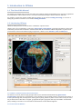
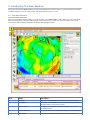
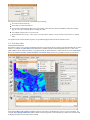
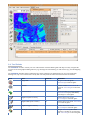
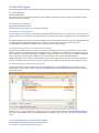
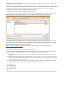
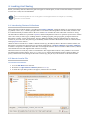
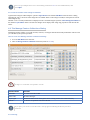
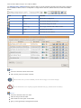
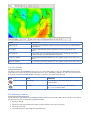
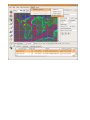
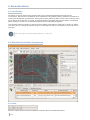
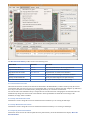
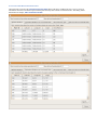
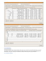
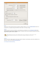
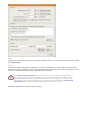
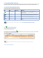
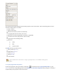
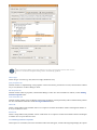
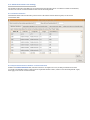
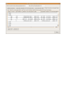
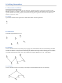
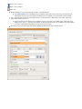
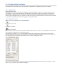
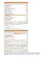
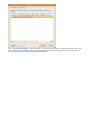
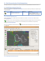
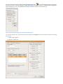
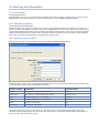
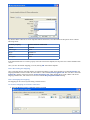
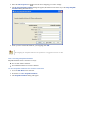
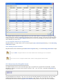
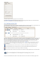
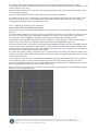
The GPlates User Manual
Rhi McKeon, James Boyden, James Clark
July 2010
GPlates User Manual
Table of Contents
1. Introduction to GPlates
1.1. The Aim of this Manual
1.2. Introducing GPlates
1.3. GPlates Development
1.4. Further Information
2. Introducing The Main Window
2.1. The Main Window
2.2. Reconstruction View
2.3. The Menu Bar
2.4. Tool Palette
2.5. List of Menu Operations
3. Data File Types
3.1. Introduction
3.2. Rasters in GPlates
3.3. Time-Dependent Global Raster Sets
4. Loading And Saving
4.1. Introducing Feature Collections
4.2. How to Load a File
4.3. The Manage Feature Collections Dialog
4.4. File Errors
5. Controlling The View
5.1. View Menu
5.2. Reconstruction View
5.3. Tool Palette
5.4. Colouring Features
6. Reconstructions
6.1. Introduction
6.2. Main Window Interface Components
6.3. Reconstruction Menu
6.4. Animations
7. Interacting With Features
7.1. Tools for Interacting with Features
7.2. Choose Feature Tool
8. More on Reconstructions
8.1. Theory
8.2. Specify Anchored Plate ID
8.3. Reconstruction Pole Dialog
9. Editing Geometries
9.1. Geometries in GPlates
9.2. Geometry-Editing Tools
9.3. In the Feature Properties Dialog
10. Creating New Features
10.1. Digitisation
11. Total Reconstruction Pole Manipulation
11.1. Modify Reconstruction Poles Tool
12. Working with Shapefiles
12.1. Introduction
12.2. Shapefile attributes
12.3. More about the Shapefile format
13. Topology Tools
13.1. Introduction
13.2. Topology Controls and Displays
13.3. Topology Sections Table
13.4. Topology Drawing Conventions
13.5. Build Topology Tool
13.6. Edit Topology Tool
1. Introduction to GPlates
1.1. The Aim of this Manual
The GPlates user manual aims to provide the reader with an almost complete understanding of the operations, applications
and manipulations within GPlates software. The manual is divided into chapters based on function and tasks.
For example, a step-by-step guide to loading data into GPlates can be found in Loading and Saving; an overview of
editing the geometries of features can be found in Editing Geometries.
1.2. Introducing GPlates
GPlates is desktop software for the interactive visualisation of plate-tectonics.
GPlates offers a novel combination of interactive plate-tectonic reconstructions, geographic information system (GIS)
functionality and raster data visualisation. GPlates enables both the visualisation and the manipulation of plate-tectonic
reconstructions and associated data through geological time. GPlates runs on Windows, Linux and MacOS X.
1.2.1. What is a Plate-Tectonic Reconstruction?
The motions of tectonic plates through geological time may be described and simulated using plate-tectonic
reconstructions. Plate-tectonic reconstructions are the calculations of the probable positions, orientations and motions of
tectonic plates through time, based upon the relative (plate-to-plate) positions of plates at various times in the past which
may be inferred from other data. Geological, geophysical and paleo-geographic data may be attached to the simulated
plates, enabling a researcher to trace the motions and interactions of these data through time.
1.2.2. The Goals of GPlates
to handle and visualise data in a variety of geometries and formats, including raster data
to link plate kinematics to geodynamic models
to serve as an interactive client in a grid-computing network
to facilitate the production of high-quality paleo-geographic maps.
1.3. GPlates Development
GPlates is developed by an international team of scientists, professional software developers and post graduate students at:
the EarthByte Project (part of the AuScope National Collaborative Research Infrastructure Strategy (NCRIS)
Program) in the School of Geosciences at the University of Sydney (under the direction of Prof. Dietmar Müller)
the Division of Geological and Planetary Sciences at CalTech (under the direction of Prof. Michael Gurnis)
the Centre for Geodynamics at the Norwegian Geological Survey (NGU) (under the direction of Prof. Trond
Torsvik).
Collaborating scientists at the University of Sydney, the Norwegian Geological Survey and CalTech have also been
compiling sets of global data for plate boundaries, continental-oceanic crust boundaries, plate rotations, absolute reference
frames and dynamic topography.
GPlates is free software (also known as open-source software), licensed for distribution under the GNU General Public
License (GPL), version 2.
1.4. Further Information
For more information about GPlates, contact us: http://www.gplates.org/contact.html
2. Introducing The Main Window
This section describes the Main Window, the heart of the GPlates user interface. Below we present annotated screenshots
of GPlates, label the key areas of the window, and provide a brief overview of each.
2.1. The Main Window
When you start GPlates, the first window you will encounter is the Main Window. This contains your view of the globe,
and is the starting-point of all tasks within GPlates. It is here that you can control your view of the globe, choose your
reconstruction time, load and unload data, and interact with geological features.
Item
Name
Description
1
Menu Bar
This region of the Main Window contains the titles of the menus.
2
Tool Palette
A collection of tools which are used to interact with the globe and
geological features via the mouse pointer.
3
Time Controls
A collection of user-interface controls for precise control of the
reconstruction time.
4
Animation Controls
A collection of tools to manipulate the animation of reconstructions.
5
Zoom Slider
A mouse-controlled slider which controls the zoom level of the
Globe View camera.
6
Task Panel
Task-specific information and controls which correspond to the
currently-activated tool.
7
View Control
Controls which projection is used to display data and the exact
zoom level as a percentage.
8
Camera Coordinate
An information field which indicates the current globe position of
the Globe View camera.
9
Mouse Coordinate
An information field which indicates the current globe position of
the mouse pointer.
10
Clicked Geometry Table
Displays a summary of each geometry or feature touched by the last
mouse click.
The appearance of the Main Window - particularly the layout of the different window
components - will change as GPlates continues to evolve.
2.2. Reconstruction View
The reconstruction view provides the user with a display of their data on the GPlates globe or map reconstructed to a
moment in time. Control of the current reconstruction time, is located under the menu bar on the left, (see image below).
The time can be controlled by both a text field, forwards and backwards time buttons, and the animation slider. In addition
the shortcut Ctrl+T to enter a time value in the text field.
2.2.1. Camera Control
When the
Drag Globe tool is activated the GPlates globe can be re-oriented freely using the mouse with a simple
click and drag motion. If another tool is selected the globe can still be dragged by holding down Ctrl.
If the user wishes to adjust the camera position to a particular latitude and longitude, pressing Ctrl+L will pop up a
window allowing manual entry of coordinates.
The amount of camera zoom can be controlled by the following:
Zoom In via mouse-wheel up.
Zoom Out via mouse-wheel down.
Zoom Control field allowing direct entry of percentage value (between 100% and 10000%). Click the text field,
type in a new value and press Enter to change the zoom.
Zoom Slider, which works on a power scale.
Keyboard shortcuts: use the + and - keys to zoom in and out, and the 1 key to reset the zoom level to 1:1 (100%)
scale.
The position of the camera and mouse pointer are provided along the bottom of the reconstruction view.
2.3. The Menu Bar
Each item in a menu is an operation. Related operations are grouped into menus, with the menu title indicating the common
theme. For example, the View Menu in the image below contains operations which manipulate the user’s view of the
globe. Within a menu, similar operations are grouped visually by horizontal lines or within sub-menus. In the View Menu
below, the Camera Location, Camera Rotation, and Camera Zoom controls are grouped into their own sub-menus.
In the Layers Menu and Geometry Colours sub menu, check boxes are displayed to switch or choose operations. For
example; Show Background Raster and the different colouring options are be activated by a small cross or tick that will
be displayed in the box in the menu when selected.
2.4. Tool Palette
The Tool Palette is used to control your view and interaction with the GPlates globe and maps. You may recognise the
concept of tools from graphics editing software (e.g. drawing tools in Photoshop ) or GIS software (e.g. ArcGIS mapping
tools).
The Tool Palette includes camera positioning tools, feature selection tools and drawing tools. A tool is activated by
clicking on it; only one tool can be active at any time. The task panel will reflect the current tool that is activated.
Item
Tool
Shortcut
Operation
Drag Globe
D
Drag to re-orient the globe.
Shift+drag to rotate the globe
Zoom In
Z
Click to zoom in. Shift+click to
zoom out. Ctrl+drag to re-orient the
globe
Choose Feature
C
Click a geometry to choose a feature.
Shift+click to query immediately.
Ctrl+drag to re-orient globe
Digitise Polyline Geometry
L
Click to draw a new vertex.
Ctrl+drag to re-orient the globe
Digitise Multi-point Geometry
M
Click to draw a new point. Ctrl+drag
to re-orient the globe
Digitise Polygon Geometry
G
Click to draw a new vertex.
Ctrl+drag to re-orient the globe
Modify Reconstruction Poles
R
Drag or Shift+drag the current
geometry to modify its reconstruction
pole. Ctrl+drag to re-orient the globe
Move Vertex
V
Drag to move a vertex of the current
feature. You can still drag the globe
around by holding down Ctrl
Insert Vertex
I
Insert a new vertex into the feature
geometry
Delete Vertex
X
Remove a vertex from a multi-point,
polyline or polygon geometry
2.5. List of Menu Operations
Tables of shortcuts and accelerators can be found in Appendix A of the user manual
A description of the operations within each menu will be explained in further detail in their respective chapters
Clicking on a menu item from the list below will take you to the appropriate chapter for further
information
2.5.1. File
Open Feature Collection
Open Raster
Open Time-dependent Raster Sequence
View Read Errors
Manage Feature Collections
View Shapfile Attributes
2.5.2. Edit
Query Feature
Edit Feature
Undo
Redo
Clear Selection
2.5.3. View
Set Projection
Camera Location
Set Location
Move Up
Move Down
Move Left
Move Right
Camera Rotation
Rotate Clockwise
Rotate Anti-clockwise
Reset Orientation
Camera Zoom
Set Zoom
Zoom In
Zoom Out
Reset Zoom
Export Geometry Snapshot
2.5.4. Reconstruction
Reconstruct to Time
Step Backward One Frame
Step Forward One Frame
Reset Animation
Play Animation
Configure Animation
Specify Anchored Plate ID
View Total Reconstruction Pole
Export Animation
Export Reconstruction Geometries
2.5.5. Layers
Geometry Colours
Plate ID
Single Colour
Feature Type
Feature Age
Show Background Raster
Set Raster Surface Extent
3. Data File Types
3.1. Introduction
This chapter covers the visualisation techniques within GPlates: which image formats are able to be loaded into GPlates
and how to go about doing this.
3.2. Rasters in GPlates
GPlates has the facility to display raster images on the globe.
3.2.1. What are raster images?
A raster image is one formed by a 2-dimensional rectangular grid coloured by points. A single point of colour in the raster
image is known as a pixel. Each pixel is positioned at one of the grid-points, and every grid-point has a pixel positioned on
it.
The ability to display raster images on the globe enables the user to superimpose any kind of imagery or gridded data (such
as satellite imagery, topography, bathymetry etc) on the surface of the globe, to be viewed at the same time as
reconstructible features. (Note that GPlates is not yet able to reconstruct raster images).
3.2.2. Which image formats does GPlates understand?
GPlates is able to display global (covering the whole globe) and regional (covering a user-specified zone) raster images.
GPlates assumes that a global image spans the longitude range of -180 degrees to +180 degrees and the latitude range of 90 to +90 degrees, and positions the image accordingly. For regional rasters a surface extent of any longitude and latitude
range for the raster can be specified, enabling rasters of a smaller size to be correctly sized and positioned.
GPlates reads images in the widely-used JPEG image format (without the need for it to be geo-referenced), enabling the
creator of an image to choose the amount of image compression used, and thus control the size of the image file created.
3.2.3. How do I load a raster image in GPlates?
A global raster image is loaded using the operation Open Raster in the GPlates File Menu. This will show a dialog
requesting the user to choose the raster image file to be loaded. When a raster image is loaded, it will replace the current
raster image (if any).
Whether or not a currently-loaded raster is displayed can be controlled using the operation Show Background Raster in
the GPlates Layers Menu. Please note that raster images do not display while using map projections other than the 3D
Globe.
3.3. Time-Dependent Global Raster Sets
3.3.1. What is a time-dependent raster set?
GPlates has the facility to display time-dependent global raster images (that is, global raster images whose pixels change
according to the reconstruction time).
In reality, what GPlates is displaying is a time-sequence of raster images — each image in the sequence corresponding to a
particular instant in geological time. The user can instruct GPlates to load a sequence of raster image files contained within
a single folder, and GPlates will display the appropriate image for the reconstruction time. As the user changes the
reconstruction time, the raster image on the globe will update accordingly.
3.3.2. How do I load an existing time-dependent raster set?
A time-dependent raster set is loaded using the operation Open Time-dependent Raster Sequence in the GPlates File
Menu. This will show a dialog requesting the user to choose the folder containing the time-dependent rasters.
A time-dependent raster set is treated the same as a regular raster image by GPlates, in the sense that when a new raster
image or time-dependent raster set is loaded, it will replace the current raster image or time-dependent raster set (if any).
Furthermore, whether or not a currently-loaded time-dependent raster set is displayed is also controlled by the operation
Show Background Raster in the GPlates Layers Menu.
Links to existing time-dependent raster sets may be found on the "Downloads" page of the GPlates website:
http://www.gplates.org/downloads.html
3.3.3. How can I create my own time-dependent raster set?
As already described, a time-dependent raster set is actually a sequence of raster image files contained within a single
folder. The name of the folder is unimportant, but the raster image files must adhere to three rules:
1. Each raster image file must be in a raster image format which GPlates is able to handle — currently only JPEG is
supported.
2. Each raster image file must have a file-name of the form “_name_-time.jpg” or “_name_-time.jpeg”, where time is
an integer value representing a number of millions of years before the present day — this is the instant of geological
time to which that raster image corresponds.
3. All raster image files in the folder must have the same name component, followed by a hyphen before the integer.
(This name component can contain further hyphens and numbers if desired.)
For example, the files:
topography-0.jpg
topography-1.jpg
topography-2.jpg
together form a time-dependent raster set. In the above example the image lasts from 0-2Ma and has "time steps" of 1Ma.
4. Loading And Saving
Before you load any data into GPlates the globe will appear as a blank sphere; in order to start with GPlates you will need
to know how to load, save and unload data.
You can still manipulate the view of the globe even though it’s blank. See Chapter 5, Controlling
the View for more details.
4.1. Introducing Feature Collections
When a data file is loaded in GPlates, it is loaded in the Feature Collection. All data in GPlates are represented as features
(e.g. MOR, volcano, etc) — whether geological data or reconstruction data. Regardless of the file format, all features will
be contained internally as GPlates features. However GPlates will remember the name and format of the file for saving.
All data loaded in GPlates are represented as features; all data-manipulation functions are operations upon features. GPlates
offers a rich variety of feature types, enabling GPlates to handle geographic, paleo-geographic, geological and tectonic
data. Basin, Coastline, Craton, Fault, Hotspot, Isochron, Mid-Ocean Ridge, Seamount, Subduction Zone, Suture and
Volcano are just some of the many feature types handled by GPlates. The meta-data attributes of data are contained within
named properties of the features.
GPlates is able to load and save a number of data-file formats (e.g. PLATES4). When a data file is loaded in GPlates, the
data will be converted to the appropriate types of features and placed into a Feature Collection. One Feature Collection
in GPlates corresponds to one data file on the disk. Even though the data have been converted to GPlates features, GPlates
will remember the name and original format of the file for saving.
When the features are saved, they will be converted back to their original data format. It is also possible to save features
into different data formats using the "Save As" or "Save a Copy" buttons in the Manage Feature Collections dialog. To
specify a different file format, change the file-name extension (e.g .dat .pla etc) to the extension for the desired format.
4.2. How to Load a File
To load files into GPlates:
1. Go to the File Menu in the menu bar.
2. Scroll down to Open Feature Collection (shortcut: Ctrl+O).
3. A classic File Open dialog window will appear; select the file to be loaded.
You can open multiple files at once via this dialog. Hold down Ctrl to select additional files, then
click Open.
4.2.1. How do I load a raster image in GPlates?
A global raster image is loaded using the operation Open Raster in the GPlates File Menu. This will show a dialog
requesting the user to choose the raster image file to be loaded. When a raster image is loaded, it will replace the current
raster image (if any).
Whether or not a currently-loaded raster is displayed can be controlled using the operation Show Background Raster in
the GPlates Layers Menu. Please note that raster images do not display while using map projections other than the 3D
Globe.
4.3. The Manage Feature Collections Dialog
This dialog window enables you to load new files, and save, reconfigure and unload currently-loaded files. This is where
you will find any file-specific operations.
How to show The Manage Feature Collections Dialog:
1. Go to the File Menu in the menu bar.
2. Click on Manage Feature Collections menu item (shortcut: Ctrl+M).
A single row in the table corresponds to one file.
Column Name
Function
File Name
The name of the file on disk
File Format
The file format type
Layer Types
Whether the file is in use on the globe canvas or being used for the rotation hierarchy
Actions
A collection of operations relevant to this file
If you place your mouse over the file name a tool tip appears indicating the directory the file is
located in.
4.3.1. Saving
There are three different ways to save a file in GPlates.
The Manage Feature Collections dialog contains a table of controls and status information about the feature collections
that are loaded in GPlates; each row corresponds to a single feature collection, and lists file name, format and available
actions.
Item
Name
Function
File Properties
Edit the file’s configuration
Save
Save the file using the current name
Save As
Save the file using a new name
Save a Copy
Save a copy of the file with a different name
Refresh
Reload the file from disk
Eject
Unload the file from GPlates
Save…
saves the current file with its current name.
will overwrite previous contents of the file.
This is useful when you have modified your file and are happy to save these changes.
Do not edit the file in two separate programs simultaneously (e.g. GPlates and a text-editor)
Save As…
saves the current file with a new name.
will leave the previous file intact.
will load the new file in place of the old file.
gives you the opportunity to change the file format.
This is useful when you want to edit a copy of a file without changing the original.
Save a Copy…
saves a copy of the current file with a new name.
will leave the previous file intact.
will not replace or unload the current file.
gives you the opportunity to change the file format.
This is useful for making backups of your work as you go.
4.4. File Errors
4.4.1. Introduction
File read errors may occur when attempting to load data from file (or some other data source, such as a database). GPlates
developers have done their best to notify the user of the specifics of the error so corrections can be made.
4.4.2. Error Categories
It is anticipated that file input errors may fall into four categories:
1. Warning
2. Recoverable error
3. Terminating error
4. Failure to begin
Warning
A warning is a notification of a problem (generally a problem in the data) which required GPlates to modify the data
in order to rectify the situation.
Examples of problems which might result in warnings include:
Data which are being imported into GPlates, which do not possess quite enough information for the needs of
GPlates (such as total reconstruction poles in PLATES4 rotation-format files which have been commented-out
by changing their moving plate ID to 999).
An attribute field whose value is obviously incorrect, but which is easy for GPlates to repair (for instance,
when the Number Of Points field in a PLATES4 line-format polyline header does not match the actual
number of points in the polyline).
A warning will not have resulted in any data loss, but you may wish to investigate the problem, in order to verify
that GPlates has corrected the errors in the data in the way you would expect; and to be aware of incorrect data
which other programs may handle differently.
Recoverable error
A recoverable error is an error (generally an error in the data) from which GPlates is able to recover, although some
amount of data had to be discarded because it was invalid or malformed in such a way that GPlates was unable to
repair it.
Examples of recoverable errors might include:
When the wrong type of data encountered in a fixed-width attribute field (for instance, text encountered where
an integer was expected).
When a recoverable error occurs, GPlates will do the following:
Retain the data it has already successfully read.
Discard the invalid or malformed data (which will result in some data loss) .
Continue reading from the data source. GPlates will discard the smallest possible amount of data, and will
inform you exactly what was discarded.
Terminating error
A terminating error halts the reading of data in such a way that GPlates is unable to read any more data from the data
source.
Examples of terminating errors might include:
A file-system error.
A broken network connection.
When a terminating error occurs, GPlates will retain the data it has already read, but will not be able to read any
more data from the data source.
Failure to begin
A failure to begin has occurred when GPlates is not even able to start reading data from the data source.
Examples of failures to begin might include:
The file cannot be located on disk or opened for reading.
The database cannot be accessed; no network connection could be established.
In the event of a failure to begin, GPlates will not be able to load any data from the data source.
5. Controlling The View
This chapter provides an overview of how to manipulate the view of the globe, and any displayed data or features.
5.1. View Menu
The View Menu enables the user to manipulate the globe, and includes the following options:
5.2. Reconstruction View
The Reconstruction View is the region of the GPlates interface which deals with plate reconstructions back through time
and is displayed below.
Name
Description
Time Controls
A collection of user-interface controls for precise control of the reconstruction time
and animations.
Zoom Slider
A mouse-controlled slider which controls the zoom level of the Globe View
camera.
View Controls
A drop-down control for selecting the projection to be used for the view, and a
precise percentage control for the camera zoom level
Camera Coordinate
An information field which indicates the current globe position of the Globe View
camera
Mouse Coordinate
An information field which indicates the current globe position of the mouse cursor
5.3. Tool Palette
The first two tools in the Tool Palette control your view of the GPlates globe or map. The Tool Palette includes camera
positioning tools, feature selection tools and drawing tools. A tool is activated by clicking on it; only one tool can be active
at any time. The Current Feature Panel will change to reflect the current tool that is activated.
Item
Tool
Operation
Drag Globe
Click and drag to re-orient the globe. Shift+drag to
rotate the globe
Zoom In
Click to zoom in. Shift+click to zoom out.
Ctrl+drag to drag the globe
5.4. Colouring Features
Found under the Layers Menu, in the Geometry Colours sub-menu, this operation allows the user to choose how feature
geometries are coloured. Current colouring methods include:
1. Colour by plate ID
2. Colour by feature age (the time of the feature’s creation relative to the current view time)
3. Colour by feature type
4. Colouring all features with a single user-specified colour.
6. Reconstructions
6.1. Introduction
The motions of tectonic plates through geological time may be described and simulated using plate-tectonic
reconstructions. Plate-tectonic reconstructions are the calculations of the probable positions, orientations and motions of
tectonic plates through time, based upon the relative (plate-to-plate) positions of plates at various times in the past which
may be inferred from other data. Geological, geophysical and paleo-geographic data may be attached to the simulated
plates, enabling a researcher to trace the motions and interactions of these data through time.
Geological time instants in GPlates are measured in units of Mega-annum (Ma), in which 1 Ma is equal to one million
years in the past. For example, the allowable range for reconstructions is from 0 to 10 000 Ma (i.e. present day to 1010
years ago).
The current age of the Earth is approximately 4.5 x 10 9 years!
6.2. Main Window Interface Components
6.2.1. Slider
Interface to interact with reconstruction animations in GPlates, discussed in further detail below.
Play
Starts animation, when pressed it changes to the pause button
Pause
Halts animation, when pressed it changes to play button
Reset
Returns animation to the start time
Fast Forward
Step forwards one frame in the animation
Rewind
Step backwards one frame in the animation
6.2.2. Step Forwards One Frame / Step Backwards One Frame (Fast Forward and Rewind):
These buttons are used to change the current reconstruction time that you are viewing in small steps. Pressing the buttons
once, or using their shortcut keys (Ctrl+I for forwards; Ctrl+Shift+I for backwards) will adjust the reconstruction time
by one frame. The time interval between frames can be adjusted via the Animate Dialog or the Specify Time Increment
dialog. Both of these can be accessed via the Reconstruction menu.
The Step Forwards one Frame / Step Backwards one Frame buttons can be held down to move
through time rapidly.
The forwards and backwards buttons apply relative to the current animation time. Normally, the present day (0 Ma) is at
the right-hand side of the animation slider, and the distant past is on the left-hand side.
GPlates makes it possible for you to set a reverse animation, where the start time is the present day (or near past), and the
end time is in the distant future. When an animation is set up this way, the slider and buttons behave as consistently as
possible; your start time (the present) is on the left, and your end time (the distant past) is on the right. Using the Step
Forwards one Frame button moves the slider to the right (into the past), and the Step Backwards one Frame button
does the opposite, as you would expect.
The default settings for the Slider are: a time range of 140Ma to present and a time increment per
frame of 1 million years
6.3. Reconstruction Menu
The Reconstruction Menu provides access to the following tools:
Menu Item
Shortcut
Operation
Reconstruct to Time
Ctrl+T
Show a reconstruction for the user-specified time
Step Forward One Frame
+ Ctrl+I+
Step forward one frame in the animation
Step Backward One Frame
Ctrl+Shift+I
Step backward one frame in the animation
Animate
Pop up the Animate dialog to control the animation
Specify Anchored Plate ID
Specify the anchored plate in the plate hierarchy
View Total Reconstruction Poles
Pop up the Total Reconstruction Poles dialog
6.3.1. Reconstruct to Time
When this menu item is invoked, it will activate the Time field in the Main Window, which is used to specify the current
reconstruction time. The user can type a new reconstruction time, or increase or decrease the value using the Up and Down
arrow keys or the mouse scroll-wheel, before pressing the Enter key to execute the reconstruction.
The current frame of the animation always corresponds to the reconstruction time. Changing the reconstruction time will
simultaneously change the current frame of the animation. If the specified time is outside the current range of the
animation, the range will be extended.
6.3.2. Step Forward One Frame
This button is used to change the current reconstruction time forward that you are viewing in small steps.
6.3.3. Step Backward One Frame
This button is used to change the current reconstruction time backward that you are viewing in small steps.
6.3.4. Specify Anchored Plate ID
This item is used to choose the anchored plate ID of the plate hierarchy. It will be described in the chapter, More On
Reconstructions.
6.3.5. View Total Reconstruction Poles
When this item is activated, the Total Reconstruction Poles dialog will appear, enabling the user to view a variety of
information about the reconstruction poles and the plate hierarchy at the current reconstruction time. This dialog will be
described in the chapter, More On Reconstructions.
6.4. Animations
The animation dialog, found in the Reconstruction menu, allows you to automate a reconstruction backwards or forwards
through time. The user can set the start and end times by either entering the age or using the current time displayed in the
main window. The options, frames per second can be set and there is also the option to loop the animation.
6.4.1. Animation Dialog
Range
This group of controls specifies the time range that the animation should cover. The Use Main Window buttons are a
convenient way of quickly entering the time that the main window is currently viewing.
Options
Additional options to fine-tune the behaviour of the animation are presented here. The Frames per second number
controls the rate at which GPlates will limit the display of animation frames when presenting an animation interactively.
Larger numbers produce a slower animation.
If calculating the next step of the animation takes too long, perhaps due to a large amount of data,
GPlates may skip some frames to try and keep the animation running at the correct rate.
Playback
These controls allow simple playback and seeking within the animation from this dialog. They behave identically to the
equivalent controls found in the Reconstruction View.
6.4.2. Export Animation Dialog
Range
This group of controls specifies the time range that the animation should cover, and are identical to the controls found in
the Animate Dialog.
Options
The Export Animation dialog briefly summarises the current export settings here. A list box shows what files will be
created at each frame of animation, along with the substitution pattern that will be used to create each unique file name.
Below that, a label indicates which directory all the files will be created in.
The Finish exactly on end time checkbox is important if you are creating an animation with a
time increment that is not an exact multiple of the range of your animation. For example, creating
an animation between 18 Ma and 0 Ma, in increments of 5 M. This range leaves a 3 million year
gap at the end which does not fit neatly into the supplied 18-0 range. Checking the Finish exactly
on end time option ensures that GPlates will still write this final, shorter, frame.
Clicking the Options button opens the following dialog:
You may type a directory name directly, or use the Choose button to navigate to one. This directory will be used to contain
all the files created from the animation export.
Below that are checkboxes to enable or disable the creation of different types of exported data, per animation step.
Export
The last group of controls in the Export Animation dialog are used to start and stop the export, and provide feedback
during the export process. Click Begin to commence the animation and begin creating files. If you have specified a large
range, this may take some time.
Once all animation frames have been processed, GPlates will stop animating and control will return to normal. The Abort
button is provided in the event that the user wishes to terminate the export sequence early.
7. Interacting With Features
This chapter provides a guide to interacting with the geological features which you are creating or editing in GPlates.
7.1. Tools for Interacting with Features
To interact with features, the following tools can be used:
Item
Tool
Shortcuts
Operation
Choose Feature
F
Click a geometry to choose a feature (being sure to be
precise). Shift+click to query immediately. Ctrl+drag to
re-orient the globe
Move Vertex
V
Drag the vertices of the currently-chosen feature. NOTE: This
tool can only be activated when a feature has been chosen.
Insert Vertex
I
Insert a new vertex into the feature geometry
Delete Vertex
X
Remove a vertex from a multi-point, polyline or polygon
geometry
To review information on all Tools please consult the Introducing the Main Window Chapter.
7.2.
Choose Feature Tool
7.2.1. Clicked Geometry Table
You can query a feature, by first selecting
then click the mouse cursor on what you want to query. The information
will be displayed in the Clicked Geometry Table.
The table will list all features that have geometry in proximity to the point that was clicked.
7.2.2. Current Feature Panel
The Current Feature Panel summarises the pertinent properties of the current feature. This is the starting point for further
interaction with the feature. It contains:
Type of feature
Name of the feature
Plate ID of the feature (used for reconstruction)
Conjugate plate ID of the feature, if it has one
Plate IDs for the left and right sides of the feature, if applicable
Life-time of the feature (the period for when it exists)
The purpose of the clicked geometry
Buttons to:
Query
Edit
Unselect feature
The Edit menu also provides access to:
Query Feature (Ctrl+Y)
Edit Feature (Ctrl+E)
Undo (Ctrl+Z)
Redo (Ctrl+R)
Clear Selection
The valid life-time of the feature is a range of geological time, i.e from 65Ma to 0Ma (present
day).
7.2.3. Querying Feature Properties
To query the properties of the current feature, either click ,
, at the bottom of the Current Feature Panel, or press
Ctrl+Y to invoke the corresponding operation in the Edit Menu. The Feature Properties dialog will appear, containing a
complete listing of the properties of the current feature.
You can keep this dialog open and continue to use the Choose Feature Tool to click on new
features - the Feature Properties dialog will be automatically updated.
Feature Type
This is the type of feature (e.g. fault, mid ocean ridge, subduction zone).
Query Properties Tab
This tab contains a complete listing of the properties of the current feature, presented in a concise, structured form which is
easy to read, but does not allow editing of values.
Edit Properties Tab
This tab contains a table of properties, which enable editing of values. For more information on this tab, consult Editing
Feature Properties below.
View Coordinates Tab
This tab contains a listing of the coordinates of the feature geometries, in both present-day and reconstructed-time position.
For more information on this tab consult Viewing Coordinates below.
Feature ID
This is a unique label for this particular feature. It is a sequence of letters and numbers which is meaningful to GPlates. It
is not yet of interest to users.
Revision ID
This is a unique label for this particular version of this feature. It is a sequence of letters and numbers which is meaningful
to GPlates. It is not yet of interest to users.
7.2.4. Editing Feature Properties
This sequence of screenshots, first shows the initial window that will appear, and the following images display the options
provided after selecting a property to edit. Each type of property has its own editing options.
The table in the centre lists all the properties belonging to the currently-chosen feature. The left hand column lists property
names, and the right hand column lists property values.
The name of a property is a way to associate meaning with the feature data - for instance, this feature has a plate ID
associated with it. That plate ID is 308. It is stored in the gpml:reconstructionPlateId property, indicating that GPlates
should use that plate ID to reconstruct the feature.
Clicking a row of the table will expand the bottom half of the dialog with new controls specific to the property that was
clicked.
7.2.5. Editing Geometry
For further information on editing feature geometries please read the Editing Geometries chapter.
The controls for directly editing the coordinates used by geometry appears as a table with Lat, Lon, and Actions columns.
Click a row of the table to select it, and the following action buttons will appear:
Insert a new row above
Insert a new row below
Delete row
Double-clicking an entry in the table lets you edit a coordinate directly.
The Valid Geometry line will indicate if the coordinates in the table can be turned into correct geometry. It
will indicate an error if there is something invalid about the coordinates, such as a lat/lon of 500 or similar.
The "Append Points" spin-boxes are designed to be a convenient means of data entry, if you need to enter some
points from a hard copy source.
Click in the Lon to start entering new coordinates. Type in a lon value, press TAB, type in a lat value, press
TAB (to move to the "+" button), press SPACE to activate that button. The new coordinate line will be added
to the table, and GPlates will prepare to receive the next line of input.
Selecting a property from the table and selecting Delete will delete the property from the feature.
7.2.6. Adding a Feature Property
By clicking on Add Property in the Feature Properties window, a new dialog will appear where you can select the
Name, Type and Value of a property. In most cases, you will only need to select the name of the property you wish to
add; the type of that property will be filled in automatically for you.
In the image above, the user has clicked on the down arrow of the combo box, and is selecting the "gpml:leftPlate"
property. This property is used to annotate which regions are on either side of features such as a mid ocean ridge.
With the property name chosen, the lower section of the dialog presents the appropriate controls for entering the new value
- in this case, a plate ID. Press Enter or the OK button to confirm the addition of the new property.
7.2.7. Viewing Coordinates
The View Coordinates dialog provides a tree view summarising the coordinates of every geometry in the feature.
The Property Name column lists the names and types of geometry, plus an enumeration of each coordinate. The Present
Day column lists the coordinates of the geometry as it appears in the present, i.e. 0 Ma. The Reconstructed column lists
the coordinates of the geometry as they appear on screen at the current view time, which for convenience is displayed at
the bottom of the dialog.
8. More on Reconstructions
8.1. Theory
8.1.1. Plate IDs
As discussed earlier in this documentation, GPlates uses the concept of a Plate ID to ascribe tectonic motion to a feature.
All features using the same plate ID move in unison when reconstructed back through time. A plate ID is a non-negative
whole number. Assigning specific meanings to specific plate IDs, such as making plate ID 714 correspond to northwest
Africa, is up to the creator of the rotation file.
Plate IDs do not correspond to a physical tectonic plate, although they may represent the motion of features which are on
that physical plate. Plate IDs can also be assigned to represent the motion of things on the same physical plate relative to
one another - for example, the motion of an island arc caused by back-arc spreading. A subduction zone can be assigned
one plate ID, and its associated island arc can be assigned another plate ID. The motion of both of these plate IDs can be
anchored to a third plate ID, representing the global motion of the physical plate underneath the subduction zone and island
arc.
8.1.2. Finite Rotations
Euler’s Displacement Theorem tells us that any displacement on the surface of the globe can be modelled as a rotation
about some axis. This combination of axis and angle is called a finite rotation. Finite rotations are used by GPlates as the
elementary building blocks of plate motion.
8.1.3. Total Reconstruction Poles
Total Reconstruction Poles tie finite rotations to plate motion. A total reconstruction pole is a finite rotation which
"reconstructs" a plate from its present day position to its position at some point in time in the past. It is expressed as the
combination of a "fixed" plate id, a "moving" plate id, a point in time and a finite rotation.
Reconstructions are defined in a relative fashion; A single total reconstruction pole defines the motion of one plate id (the
"moving" plate id) relative to another (the "fixed" plate id) at a specific moment in geological time. A sequence of total
reconstruction poles is needed in order to fully model the motion of one particular plate across the surface of the globe
throughout time.
8.1.4. Anchored Plate ID
A sequence of total reconstruction poles is used to model the motion of a single plate across the surface of the globe. The
total reconstruction poles describe the relative motion between each plate, but ultimately this motion has to be traced back
to a single plate ID which is considered "anchored". GPlates calls this the Anchored Plate ID. Generally, this plate ID
corresponds to an absolute reference frame, such as a hotspot, paleomagnetic, or mantle reference frame. The convention is
to assign the anchored plate ID to 000, but GPlates allows any plate ID to be used as the anchored plate ID.
8.1.5. The Rotation Hierarchy
To create the model of global plate rotations that is used in GPlates, total reconstruction poles are arranged to form a
hierarchy, or tree-like structure. At the top of the hierarchy is the anchored plate ID. Successive plate IDs are further down
the chain, linked by total reconstruction poles. To calculate the absolute rotation of a plate ID of a plate with a given plate
ID. (relative to the fixed reference defined by the anchored plate ID, at a given time), GPlates starts at that point in the
hierarchy and works its way up to the top - to the root of the tree.
8.2. Specify Anchored Plate ID
The Specify Anchored Plate ID command on the Reconstruction menu can be used to change which plate ID GPlates
considers to be the globally fixed reference when performing reconstructions. Enter a new plate ID to be the anchor in the
dialog that pops up, and GPlates will automatically rearrange the rotation hierarchy so that the specified plate ID is at the
top.
8.3. Reconstruction Pole Dialog
The Total Reconstruction Pole Dialog is accessed from the Reconstruction menu. It contains four tables of information,
relevant to the current reconstruction time and the current anchored plate ID.
8.3.1. Relative Rotations
This table lists all the total reconstruction poles in terms of the relative motions between plates, for the current
reconstruction time.
8.3.2. Equivalent Rotations Relative To Anchored Plate
Similar to the Relative Rotations table, this lists rotations for each plate. However, the data presented here has been
converted from individual relative rotations into the equivalent absolute rotation, relative to the anchored plate ID. Again,
these apply to the current reconstruction time.
8.3.3. Reconstruction Tree
Here the reconstruction hierarchy is presented in a more natural, tree-like form. Relative rotations are listed, but individual
nodes of the tree (plate IDs) can be expanded or collapsed, to explore the branches of the plate rotation model.
8.3.4. Plate Circuits To Stationary Plate
This tab of the Total Reconstruction Poles dialog can be used to trace a series of total reconstruction poles from any given
plate ID back to the top of the hierarchy, the anchored plate ID. It is useful to quickly identify the other plate IDs that a
chosen plate ID depends on.
9. Editing Geometries
9.1. Geometries in GPlates
The geometries which GPlates handles are point, multi-point, polyline and polygon. Certain types of features contain
different geometries, for example: a volcano uses a point to represent its position; a multi-point is used to represent a field
of points which all have the same properties; an Isochron uses a polyline to represent its centre-line; and a basin uses a
polygon to represent its outline.
9.1.1. Point
A point is the most basic form of geometry in GPlates and the basis of all other geometries.
9.1.2. Multi-point
A collection of points that move as one.
9.1.3. Polyline
A series of lines drawn end-to-end, forming an open polygon. It is assumed that the lines are non-intersecting. Sometimes
in GPlates the direction of a polyline is important, when determining the properties on either side of the line; for example,
one side of a subduction zone represents the subducting slab, while the other represents the overriding plate. The direction
of a polyline is determined from the "start" of the polyline (the first point digitised) to the "end" of the polyline.
9.1.4. Polygon
A series of lines drawn end-to-end, forming a closed shape. It is assumed that the lines are non-intersecting.
9.2. Geometry-Editing Tools
The geometry-editing tools are Canvas Tools and can be found in the Tool Palette. To begin editing geometries it is first
necessary to select the feature using the Choose Feature Tool,
.
The Geometry Editing Tools can only be used on the currently chosen feature.
9.2.1.
Move Vertex Tool
Once you have selected a feature, its properties will appear in the Current Feature Panel. Little dots will appear on the
chosen feature geometry, representing the vertices and can be positioned to a new location. The changes made to the
geometry are immediate and there is no need to press an "Apply" button.
This tool is useful for correcting mistakes in the features' geometry.
9.2.2.
Insert Vertex Tool
If the current geometry is a polyline or polygon, when the user clicks on a line, a new vertex is inserted at that position on
the line. This vertex may then be dragged to a new position, using the move vertex tool.
If the current geometry is a multi-point, a new point will be created at the click-position.
9.2.3.
Delete Vertex Tool
If the current geometry is a polyline or polygon, when the user clicks on an existing vertex, that vertex will be deleted. The
vertices on either side of the removed vertex will now be connected directly, creating a new polyline or polygon. In the
case of multi-point geometry, when the user clicks on an existing point, the point will be removed.
Note that if a vertex is removed from a polygon, the resulting geometry will still be a closed
polygon, as long as there are sufficient remaining vertices. GPlates requires at least three distinct
points to define a polygon. If there are only two distinct points remaining, the geometry will
become a polyline.
Note that if a vertex is removed from a polyline, the resulting geometry will still be a single
continuous polyline, as long as there are sufficient remaining vertices. GPlates requires at least two
distinct points to define a polyline. If there is only one distinct point remaining, the geometry will
become a point.
Note that if a vertex (i.e. point) is removed from a multi-point geometry which contains only two
points, it will become a point geometry.
It is invalid to remove a vertex from a single point geometry. In order to remove the geometry
entirely the feature will have to be deleted.
9.3. In the Feature Properties Dialog
The controls for directly editing the coordinates used by geometry appears as a table with Lat, Lon, and Actions columns.
Click a row of the table to select it, and the following action buttons will appear:
Insert a new row above
Insert a new row below
Delete row
Double-clicking an entry in the table lets you edit a coordinate directly.
The Valid Geometry line will indicate if the coordinates in the table can be turned into correct geometry. It
will indicate an error if there is something invalid about the coordinates, such as a lat/lon of 500 or similar.
The "Append Points" spin-boxes are designed to be a convenient means of data entry, if you need to enter some
points from a hard copy source.
Click in the Lon to start entering new coordinates. Type in a lon value, press TAB, type in a lat value, press
TAB (to move to the "+" button), press SPACE to activate that button. The new coordinate line will be added
to the table, and GPlates will prepare to receive the next line of input.
Selecting a property from the table and selecting Delete will delete the property from the feature.
10. Creating New Features
This chapter aims to provide the reader with information and instructions for digitising new features in GPlates.
10.1. Digitisation
GPlates allows the user to create features on the globe: from aseismic ridges to volcanoes. To create a new feature, a user
first "digitises" a new geometry, then specifies the additional properties for that feature. The geometries which GPlates
handles are point, polyline (a series of lines drawn end-to-end, forming an open polygon) and polygon. Certain types of
features require certain geometries, for example: a volcano uses a point to represent its position; an isochron uses a polyline
to represent its center-line; and a basin uses a polygon to represent its outline.
10.1.1. Digitisation Tools
GPlates offers three digitisation tools in the Tool Palette:
Polyline Geometry
Point Geometries
Polygon Geometry
Each tool can be used to create any of the GPlates GPML features, however it is the user’s responsibility to ensure that the
correct geometry is digitised for the intended feature type.
After choosing a geometry tool, you can begin adding control points to the globe by clicking on an area; these points
define the geometry (feature) you want to create. (You can still rotate the globe by holding down the Ctrl key.) After you
have plotted the feature, the latitude and longitude can be verified in the digitisation panel.
Once you are satisfied with the new feature location, click Create Feature button to select the type of feature you would
like to create. E.g Isochron, Fault, Mid Ocean Ridge etc.
The next step is to assign a geometry to the feature as well as:
Plate ID
A begin time for the feature
An end time
A name (To help you distinguish/classify your feature)
In the final step of feature creation, the feature is assigned to a feature collection. All data files that are currently loaded in
GPlates will be listed here, as well as the < New Feature Collection > option. Choosing any one of the existing feature
collections and clicking Create will add the newly digitised feature to that collection and return the user to the GPlates
main window.
If the < New Feature Collection > option is selected, a new feature collection will be created to hold the new feature. This
feature collection will not yet have a name, and is not associated with a file on disk. Like all other feature collections, the
new one will be found in the Manage Feature Collections dialog.
11. Total Reconstruction Pole Manipulation
This chapter describes how to manipulate the reconstruction pole hierarchy using the Modify Reconstruction Poles tool.
11.1. Modify Reconstruction Poles Tool
Found on the Tool Palette, the Modify Reconstruction Poles Tool is used to interactively modify the reconstruction poles
for a given plate ID.
Item
Tool
Shortcut
Operation
Modify Reconstruction Poles
R
Drag or Shift+drag the current
geometry to modify its reconstruction
pole. Ctrl+drag to re-orient the globe
11.1.1. Choosing a Plate ID to move
To select a Plate ID to move, the Plate needs to be in the field of view, and the reconstruction time needs to be at the
correct geological time.
The second step is to select a feature which belongs to the plate ID that should be changed. Select the Choose Feature tool,
, then click the mouse cursor on the feature. You can confirm that you have selected the correct plate ID by
checking the Current Feature Panel.
Now select the Modify Reconstruction Poles tool,
now highlighted.
11.1.2. Adjusting a Reconstruction Pole
. Notice that all features belonging to the chosen plate ID are
After the feature plate has been selected with the Choose Feature tool (
) it can be dragged anywhere on the globe.
The plate can also be rotated by holding down Shift and dragging. The globe can still be re-orientated whilst dragging the
plate by holding down Ctrl. The Task Panel will display information about the reconstruction pole.
11.1.3. Committing Changes to a Reconstruction Pole
To commit changes to a reconstruction pole, simply click Apply and a new window will open up asking
the user to:
1. Choose a pole sequence
2. Verify new relative pole
12. Working with Shapefiles
12.1. Introduction
ESRI Shapefiles are one of the recognised Feature Collection file formats in GPlates. Loading a feature collection from a
Shapefile follows the same procedure as any other feature data file - see the Loading and Saving chapter.
12.2. Shapefile attributes
Shapefile attributes can contain meta-data associated with the geospatial data. This data could specify, for example, the
feature’s reconstruction plateID, or the times of appearance and disappearance of the feature. GPlates allows you to specify
which shapefile attribute field names will be associated with GPlates feature properties, such as the reconstruction plateID.
GPlates records this information on disk so that in subsequent GPlates sessions the last used association will be loaded by
default. You can change this association at any time during a GPlates session.
12.2.1. Mapping shapefile attributes
The first time a shapefile has been loaded, you will see the Map Shapefile Attributes dialog.
This dialog allows the user to select which shapefile attribute fields will be associated with GPlates feature properties. The
feature properties are listed on the left-hand side of the dialog.
Feature property Explanation
Expected values
PlateID
The reconstrution plateID for the feature
Integer
Feature type
The type (e.g. Coastline, COB) of the feature
Two letter code
Begin
The time of appearance of the feature
Numerical
End
The time of disappearance of the feature
Numerical
Name
The name of the feature
Text
Description
A description of the feature
Text
Alongside each feature property is a drop-down box showing the name of the shapefile attribute field which will be
associated with the feature property. You can use the drop-down boxes to change the shapefile attribute fields which you
want to associate with each feature property.
By default GPlates will look for certain shapefile attribute field names, and will initialise the drop-down boxes with the
following values:
Feature property
Default attribute field name
PlateID
PLATEID
Feature type
TYPE
Begin
FROMAGE
End
TOAGE
Description
DESC
If the default field name for a feature property cannot be found in the shapefile, the drop-down box will be initialised with
<none>.
Once you have selected the mapping you want, clicking OK will load the shapefile.
12.2.2. Recording the mapping
Once a mapping has been selected, GPlates records this information on disk. If the shapefile was called mydata.shp, the
mapping information will be stored in the same folder in a file called mydata.shp.gplates.xml. The next time a user loads
mydata.shp, GPlates will look for the file mydata.shp.gplates.xml. If this mapping file is found, GPlates will use the
mapping contained in it, and will not force the user to use the Map Shapefile Attributes dialog.
12.2.3. Changing the mapping
The mapping can be reset at any time during a GPlates session.
To reset the mapping for a feature collection:
1. Open the Manage Feature Collections dialog (Ctrl+M)
2. Select the File Properties icon
for the file whose mapping you want to change.
3. The Re-map Shapefile Attributes dialog will appear; this behaves in the same way as the Map Shapefile
Attributes dialog described above.
4. When you have selected the fields for your mapping, click OK.
Re-mapping the shapefile attributes will update the *.shp.gplates.xml file on disk.
12.2.4. Viewing Shapefile attributes
Shapefile attributes can be viewed in two ways:
For an entire feature collection.
For individual features in a feature collection.
To view shapefile attributes for a feature collection
1. Go to the File Menu in the menu bar.
2. Scroll down to View Shapefile Attributes
3. The Shapefile Attributes dialog will appear.
The shapefile attribute field names are displayed at the top of each column. Each row of the table corresponds to a single
feature in the feature collection, and displays the attribute values for that feature. If there is more than one shapefile feature
collection loaded, you can use Feature Collection drop-down box at the top of the dialog to select the feature collection
whose attributes you want to view.
To view shapefile attributes for a single feature
Shapefile attributes for a single feature can be viewed through the Query Feature Properties dialog - see the Interacting
with Features chapter.
12.2.5. Editing Shapefile attributes
Shapefile attributes can be edited through the Edit Feature Properties dialog - see the Interacting with Features chapter.
Only the value of shapefile attributes can be edited. Field names and field types cannot be edited.
You cannot create new shapefile attribute fields or delete existing shapefile attribute fields.
12.3. More about the Shapefile format
The ESRI Shapefile format is a file format allowing storage of geospatial vector graphics data and metadata. An ESRI
Shapefile is a collection of (at least) 3 files with file extensions ".shp", ".shx" and ".dbf". A shapefile called mydata will
consist of the files:
mydata.shp
mydata.shx
mydata.dbf
The geospatial data are stored in the ".shp" and ".shx" files; the meta-data (attributes) are stored in the ".dbf" file. When
loading a shapefile feature collection, you only need to select the ".shp" file; the ".shx" and ".dbf" files are loaded
automatically. The file filter used in the Open Feature Collection dialog will show only the ".shp" form of shapefiles.
The ESRI shapefile specification can be downloaded from http://www.esri.com/library/whitepapers/pdfs/shapefile.pdf.
13. Topology Tools
13.1. Introduction
In GPlates, everything is a feature. Many features on the globe are reconstructable, and have an unchanging geometric
presence that is moved around the globe according to the reconstruction tree. This chapter introduces Topological features,
which do not have a geometry of their own defined.
Instead of a single fixed geometry, topological features automatically construct their geometry based on the parts of other
features. The most useful application of this is constructing topological closed plate polygons based on the intersections of
various plate tectonic boundary features.
13.2. Topology Controls and Displays
In addition to the Globe, the various Topology Tools make use of a few other displays and controls on the Main Window.
The Topology Tools Task Panel and The Topology Sections Table work together to manipulate the list of features that
form a topology’s boundary. As you edit the list of boundary features, you will work back and forth between the globe, the
Task Panel, and the Sections Table.
13.2.1. Topology Tools Task Panel
The Topology Tools Task Panel has two sub-tabs, one for the topology itself, and the other for a feature intended to
become a section of the topology.
13.2.2. Topology Tab
The Topology Tab shows a summary of the topology under edit.
When building a new topology, the Name, Plate Id, and Valid Time displays will be blank (these values will be set when
finalizing the new topology). When editing an existing topology these will display that the various property values of that
topology feature.
The Remove All Sections button will delete all entries in Topology Sections Table, and effectively clear the topology. Use
with caution this operation has no undo.
The Apply/Create… button is used to apply all edits to the current topology (under the Edit Topology Tool), or to finalise
the creation process (under the Build New Topology Tool).
13.2.3. Section Tab
The Section Tab shows the basic properties of the focused feature.
The Add Focused Feature button will insert the feature into the Topology Sections Table at the current Insertion Point.
See below for an explaination of the table and the insertion point.
13.3. Topology Sections Table
The Topology Sections Table holds an ordered list of boundary features. Upon each reconstruction, it is these features, and
their relationships, that will be processed into the resultant polygon geometry for the topology.
Features are added to the Sections Table via the controls in the Task Panel, and via the table itself. The insert location of the
table (and corresponding spot on the ordered list of boundary features) will be highlighted by a special row with a large
blue arrow and a message. This is the Insertion Point. The insertion point usually stays at the end of the list, so that each
new section gets appended to the topology one after the other. If you wish to insert a feature elsewhere in the list of
boundary sections, adjust the insertion point’s location using the buttons in the table.
All the controls for directly editing the Sections Table appear under the Actions column of the table. Buttons related to a
row will appear on mouse-over. Simply move the mouse pointer over a section in the table, and the following action
buttons will appear:
Move the Insertion Point to the row above this one; new sections will be added to the topology before this one.
Move the Insertion Point to the row below this one; new sections will be added to the topology after this one.
Remove this section from the list. It will no longer contribute to the topology.
Reset the Insertion Point to the last entry. This causes insert operations to simply append features to the Sections Table.
If you need to distinguish between similar features used in the topology, click on a row of the
table. This will highlight that row, and also highlight the corresponding geometry on screen.
The Reverse column indicates if the feature’s vertices will be used in a the reverse order from which they appear in the
source feature’s data. This is a toggle box and may be changed from the default pre-computed value if needed.
Occasionally the default state will not match the users intent, or geometric arrangement of the feature, and this box may be
used to reorder the vertex usage.
Please note: this check box has no effect on the underlying referenced data, rather it only controls how that data is used
when resolving the topology.
The Feature Type, Plate ID, and Name columns provide a quick summary of the Section.
The background colour of a row will change to red if there are some problems resolving that part of the topology. This
may occur, for example, when you have loaded a file containing the topology definitions but have yet to load a file
containing the features that were used to build that topology.
13.4. Topology Drawing Conventions
While a topology feature is under edit GPlates will draw the topology, and its referenced features, with certain highlights
and colors.
The focused feature will always be drawn in white. A large white dot will be drawn on the head vertex (the first vertex in
the feature’s current geometry), and a small white dot will be drawn on the tail vertex (the last vertex in the feature’s
current geometry). These highlights are intended to aid in the selection and ordering of boundary features.
The topology’s resultant boundary polygon will be drawn in light gray. All the topology’s resultant vertices, both those
from the source features, and those computed as intersection points, will be highlighted with gray dots.
The current Insertion Point of the Topology Section Table will be highlighted visually on the globe with slightly different
coloring of the features on either side of it: The feature before the insertion point will be drawn in Black, and the feature
after the insertion point will be drawn in White. The mnemonic before black; after white is a quick way to recall where a
new feature will be inserted into the topology sections Table.
For features with polyline geometry, the specific spot on or near the line that was actually used to select the feature (the socalled the "click-point") will be drawn with a Black dot. Point features do not have this click-point drawn since it overlaps
exactly with the point feature.
Line geometries will also have their current head vertex highlighted with a large gray dot. Please note: this current head
vertex will be the opposite of the actual data file’s head vertex if the line feature is being used in the reverse order.
If you click on the globe background or use the Clear Selection action on the Edit menu, a small dark green dot will be
drawn to highlight the last click-point. This is used for reference only.
These visual cues may be helpful when fine tuning how various features, particularly features with complicated polylines,
intersect to form a topology’s boundary.
Checkable items in the Layers menu can be used to reduce visual clutter, by switching off the
display of certain types of geometry. Remember that you can also use the Clicked Feature Table to
help you pick out features when they overlap.
13.5. Build Topology Tool
The Build Topology tool is the tool used to create new topology features from existing regular non-topological features.
You will select a series of features, in an ordered fashion, moving around the intended boundary of the topology.
13.5.1. Activate the Tool
First, click on the Build New Topology tool button. You may need to deselect a feature you are currently working on for
this tool to become available.
Initially the new topology will have an empty list of sections. As you add sections to the topology, the Topology Sections
Table will become populated with the features.
13.5.2. Select Features to become Topology Sections
Next, select a feature by clicking on it on the Globe.
You do not have to switch to the Choose Feature Tool. The Build Topology Tool is a specialised
version of choosing features.
If more than one feature is under the click point, you can use the Clicked Table to further refine your selection to the
proper feature.
Once you have identified the desired feature, click the Add Focused Feature button. The referenced feature is transferred
to the Topology Sections Table, where it will be used to construct part of the topology’s boundary.
Continue creating the intended boundary of the new topology by selecting a feature to focus it, and then clicking Add
Focused Feature to insert it into the Topology Section Table.
It is recommended to create a new topology by cycling around the boundary systematically (either a clockwise or counterclockwise) and appending features to the end of the Topology Sections Table.
13.5.3. Editing the Sections Table
If you have discovered that you forgot a feature in the middle of the boundary list list, or realise you want to modify the
ordering of the Sections in the Table, then you may change the insert point via the Actions column of the table, and
continue with the same steps as above: Focus a feature on the Globe, then click the Add Focused Feature button.
Adding a feature does not change the insertion point, so be aware if you perform an Insert operation out of sequence.
13.5.4. Creating the new feature
Once you are satisfied with the entries in the Topology Sections Table, and the resultant polygon geometry of the Topology
itself, then you may create the new Topology via the Apply/Create button on the Topology Tab of the Topology Task
Panel. This action will lead you through a series of dialogs to finalise the creation process.
In the first step you will choose the Feature Type of the new Topology. Currently GPlates supports only one type of
topology: TopologicalClosedPlateBoundary.
The next step is to assign other basic property values to the Topology.
The geometry type is usually Boundary, and this value is automatically selected for you.
The other basic feature properties must be set as well: Plate ID, Begin Time, End Time, Name.
In the final step of feature creation, the feature is assigned to a feature collection. All data files that are currently loaded in
GPlates will be listed here, as well as the < New Feature Collection > option. Choosing any one of the existing feature
collections and clicking Create will add the newly created topology feature to that collection and return the user to the
GPlates main window.
If the < New Feature Collection > option is selected, a new feature collection will be created to hold the new feature. This
feature collection will not yet have a name, and is not associated with a file on disk. Like all other feature collections, the
new one will be found in the Manage Feature Collections dialog.
The convenience button Create and Save adds the feature to the selected feature collection, and opens the Manage Feature
Collections dialog, so that you may immediately save or rename the collection.
13.6. Edit Topology Tool
The Edit Topology tool is the tool used to edit existing topology features. Under this tool you will load an exiting
topology into the Topology Sections Table, and make edits to that ordered list of features.
13.6.1. Activate the Tool
First, use the Choose Feature Tool to select an existing topology. You may have to click on the panel below to select the
topology rather than the selected line.
Next, click on the Edit Topology tool button.
13.6.2. Editing the Topology
Notice that the topology will be drawn with the highlighting described above. The feature’s basic data is placed into the
Topology tab of the Task Panel, and the Topology Sections Table will be filled with the list of boundary features.
From this point on the same basic editing steps described above, such as inserting or deleting a line, may be used to change
the Topology Sections Table (the boundary list).
Once you are satisfied with the changes, click on the Apply/Create button and the Topology’s boundary list will be
changed to the current contents of the Topology Section Table.
More advanced editing may be required with time-dependent topologies. Due to the semi-automated nature of closing
topologies a likely source of any problems that may arise is the constituting lines; namely the length and/or time of
appearance and order of inclusion in the topology. If not closed properly the polygon will fail and exhibit anomalous
vertices and skewed lines.
A handy way of checking what a final polygon looks like is by turning off the lines. This is
achieved by clicking the Layers toolbar and unticking the Show line features option.
It may be necessary to break the time period of an existing topology, for instance if a line needs to be inserted or deleted at
a particular timestep but the opposite case is true for the adjacent time period. For example, a particular topology is valid
from 20-10Ma and a constituting line included in the topology is relevant for 20-16 Ma but not 16-10Ma. With the line
inserted the topology will therefore close correctly between 20-16Ma but fail from 16-10Ma in the given scenario (the
opposite case would be true if the line was deleted from the polygon). In this case you need to duplicate the topology entry
and effectively make two new polygons with different times of appearance or disappearance i.e. one topology valid from
20-16Ma and the other from 16-10Ma.
Firstly select and highlight the topology, as previously described, and then click on the clone feature icon on the right
panel. Reclicking on the topology, you will see two copies of the topology entry in the Clicked Feature Table at the bottom
of the window. To change the validity of the feature click on the original or duplicate entry and click on the Edit feature
properties icon on the right panel, and change the Begin and/or End time. Remember to press Enter to adjust the new time
period.
For convenience of reconstruction and preventing the overlap of polygons at 1Myr timesteps, the
time of appearance may be best selected at ##.10Ma, i.e. 20.10-15.10Ma (20-16Ma) and 15.109.10Ma (15-10Ma)
You may also need to extend a line so that a topology closes. This problem often arises when using rotation files that are
significantly different, and therefore the new location of a particular plate ID-assigned line may mean that a topology is no
longer closed. This method is best restricted to instances where the line only needs to be extended a relatively short
distance and in a largely straight line. This is achieved by using the Insert Vertex icon, as previously described. Because the
topology already exists as an entry, the new line will be automatically incorporated and the topology should be successfully
closed. It is wise to check the polygons through time that utilize this line, to ensure that no other existing polygons have
been changed.
Last updated 2010-07-08 21:18:36 EST