1
Professional Graphics Language
Professional Graphics Language
Professional Graphics Language
Professional Graphics Language
Professional Graphics Language
v4.0
Professional Graphics Language
Graphics Layout Engine
User Manual (v. 4.0.13)
C. Pugmire, St.M. Mundt, V.P. LaBella, J. Struyf
http://www.gle-graphics.org/
11 September 2007
ii
Contents
vii
1 Preface
2 Tutorial
3
2.1
Installing GLE . . . . . . . . . . . . . . . . . . . . . . . . . . . . . . . . . . . . . . . . . .
3
2.2
Running GLE . . . . . . . . . . . . . . . . . . . . . . . . . . . . . . . . . . . . . . . . . . .
3
2.3
Drawing a Line on a Page . . . . . . . . . . . . . . . . . . . . . . . . . . . . . . . . . . . .
4
2.4
Drawing a Simple Graph . . . . . . . . . . . . . . . . . . . . . . . . . . . . . . . . . . . . .
5
3 Primitives
7
3.1
Graphics Primitives (a summary) . . . . . . . . . . . . . . . . . . . . . . . . . . . . . . . .
7
3.2
Graphics Primitives (in detail) . . . . . . . . . . . . . . . . . . . . . . . . . . . . . . . . .
8
4 The Graph Module
21
4.1
Graph Commands (a summary) . . . . . . . . . . . . . . . . . . . . . . . . . . . . . . . . .
21
4.2
Graph Commands (in detail) . . . . . . . . . . . . . . . . . . . . . . . . . . . . . . . . . .
22
4.3
Bar Graphs . . . . . . . . . . . . . . . . . . . . . . . . . . . . . . . . . . . . . . . . . . . .
29
4.4
3D Bar Graphs . . . . . . . . . . . . . . . . . . . . . . . . . . . . . . . . . . . . . . . . . .
30
4.5
Filling Between Lines
. . . . . . . . . . . . . . . . . . . . . . . . . . . . . . . . . . . . . .
31
4.6
Notes on Drawing Graphs . . . . . . . . . . . . . . . . . . . . . . . . . . . . . . . . . . . .
31
4.6.1
Importance of Order . . . . . . . . . . . . . . . . . . . . . . . . . . . . . . . . . . .
31
4.6.2
Line Width . . . . . . . . . . . . . . . . . . . . . . . . . . . . . . . . . . . . . . . .
31
5 The Key Module
33
5.1
Global Commands . . . . . . . . . . . . . . . . . . . . . . . . . . . . . . . . . . . . . . . .
34
5.2
Entry Definition Commands . . . . . . . . . . . . . . . . . . . . . . . . . . . . . . . . . . .
35
5.3
Defining the Key in the Graph Block . . . . . . . . . . . . . . . . . . . . . . . . . . . . . .
36
iii
iv
CONTENTS
6 Programming Facilities
37
6.1
Expressions . . . . . . . . . . . . . . . . . . . . . . . . . . . . . . . . . . . . . . . . . . . .
37
6.2
Functions Inside Expressions . . . . . . . . . . . . . . . . . . . . . . . . . . . . . . . . . .
37
6.3
Using Variables . . . . . . . . . . . . . . . . . . . . . . . . . . . . . . . . . . . . . . . . . .
39
6.4
Programming Loops . . . . . . . . . . . . . . . . . . . . . . . . . . . . . . . . . . . . . . .
40
6.4.1
Default Arguments . . . . . . . . . . . . . . . . . . . . . . . . . . . . . . . . . . . .
40
6.5
I/O Functions . . . . . . . . . . . . . . . . . . . . . . . . . . . . . . . . . . . . . . . . . . .
41
6.6
Device dependend Control . . . . . . . . . . . . . . . . . . . . . . . . . . . . . . . . . . . .
42
7 Advanced features
43
7.1
Diagrams, Joining Named Objects . . . . . . . . . . . . . . . . . . . . . . . . . . . . . . .
43
7.2
LaTEX Interface . . . . . . . . . . . . . . . . . . . . . . . . . . . . . . . . . . . . . . . . . .
44
7.2.1
Example . . . . . . . . . . . . . . . . . . . . . . . . . . . . . . . . . . . . . . . . . .
44
7.2.2
Using LaTeX Packages . . . . . . . . . . . . . . . . . . . . . . . . . . . . . . . . . .
44
7.2.3
Import in a TeX Document . . . . . . . . . . . . . . . . . . . . . . . . . . . . . . .
45
7.2.4
The .gle Directory . . . . . . . . . . . . . . . . . . . . . . . . . . . . . . . . . . . .
45
7.3
Filling, Stroking and Clipping Paths . . . . . . . . . . . . . . . . . . . . . . . . . . . . . .
45
7.4
Colour . . . . . . . . . . . . . . . . . . . . . . . . . . . . . . . . . . . . . . . . . . . . . . .
46
7.5
GLE’s Configuration File . . . . . . . . . . . . . . . . . . . . . . . . . . . . . . . . . . . .
47
8 Surface and Contour Plots
8.1
49
Surface Primitives . . . . . . . . . . . . . . . . . . . . . . . . . . . . . . . . . . . . . . . .
49
8.1.1
Overview . . . . . . . . . . . . . . . . . . . . . . . . . . . . . . . . . . . . . . . . .
49
8.1.2
Surface Commands . . . . . . . . . . . . . . . . . . . . . . . . . . . . . . . . . . . .
49
8.2
Letz . . . . . . . . . . . . . . . . . . . . . . . . . . . . . . . . . . . . . . . . . . . . . . . .
53
8.3
Fitz . . . . . . . . . . . . . . . . . . . . . . . . . . . . . . . . . . . . . . . . . . . . . . . .
53
8.4
Contour . . . . . . . . . . . . . . . . . . . . . . . . . . . . . . . . . . . . . . . . . . . . . .
54
8.5
Color Maps . . . . . . . . . . . . . . . . . . . . . . . . . . . . . . . . . . . . . . . . . . . .
55
9 GLE Utilities
57
9.1
Fitls . . . . . . . . . . . . . . . . . . . . . . . . . . . . . . . . . . . . . . . . . . . . . . . .
57
9.2
Manip . . . . . . . . . . . . . . . . . . . . . . . . . . . . . . . . . . . . . . . . . . . . . . .
58
CONTENTS
v
9.2.1
Usage . . . . . . . . . . . . . . . . . . . . . . . . . . . . . . . . . . . . . . . . . . .
58
9.2.2
Manip Primitives (a summary) . . . . . . . . . . . . . . . . . . . . . . . . . . . . .
59
9.2.3
Manip Primitives (in detail) . . . . . . . . . . . . . . . . . . . . . . . . . . . . . . .
60
A Tables
65
A.1 Markers . . . . . . . . . . . . . . . . . . . . . . . . . . . . . . . . . . . . . . . . . . . . . .
65
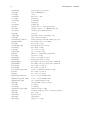
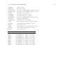
A.2 Functions and Variables . . . . . . . . . . . . . . . . . . . . . . . . . . . . . . . . . . . . .
65
A.3 LaTEX Macros and Symbols . . . . . . . . . . . . . . . . . . . . . . . . . . . . . . . . . . .
68
A.4 Installing GLE . . . . . . . . . . . . . . . . . . . . . . . . . . . . . . . . . . . . . . . . . .
69
A.5 Fonts . . . . . . . . . . . . . . . . . . . . . . . . . . . . . . . . . . . . . . . . . . . . . . . .
69
A.6 Font Tables . . . . . . . . . . . . . . . . . . . . . . . . . . . . . . . . . . . . . . . . . . . .
70
A.7 Predefined Colors . . . . . . . . . . . . . . . . . . . . . . . . . . . . . . . . . . . . . . . . .
83
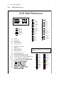
A.8 Wall Reference . . . . . . . . . . . . . . . . . . . . . . . . . . . . . . . . . . . . . . . . . .
85
Index
87
vi
CONTENTS
Chapter 1
Preface
Abstract
GLE (Graphics Layout Engine) is a graphics package for scientists, combining a user-friendly scripting
language with a full range of facilities for producing publication-quality graphs, diagrams, posters and
slides. GLE provides LaTEX quality fonts together with a flexible graphics module which allows the user
to specify any feature of a graph. Complex pictures can be drawn with user-defined subroutines and
simple looping structures. Current output formats include EPS, PS, PDF, JPEG, and PNG.
Trademark Acknowledgements
The following trademarks are used in this manual.
Windows
TEX
LaTEX
PostScript
Microsoft Corporation.
Donald E. Knuth, A Typesetting System.
Leslie Lamport, A Document Preparation System.
Page Description Language, Adobe Systems Inc.
Typographic Conventions
The following conventions will be used in command descriptions:
[option]
option1 | option2
keyword
exp,x,y,x1,y1
Specifies an optional keyword or parameter, the brackets should
not be typed.
Pick one of the options listed.
Keywords are represented in a bold typewriter font.
Represent numbers or expressions. E.g. 2.2 or 2*5. Parameters
to be entered by the user are given in italics.
Pathways
For those in a hurry:
1. Read chapter 1, The GLE Tutorial (beginners only).
vii
1
2. Examine the examples at http://www.gle-graphics.org/examples/.
3. Browse through Chapter 3, The Graph Module.
For those with time:
• Chapter 2, GLE Tutorial: Covers installation and drawing a simple graph, highly recommended
if you have never used GLE before.
• Chapter 3, GLE Primitives: Describes the commands used for creating diagrams and slides and
for annotating graphs.
• Chapter 4, The Graph Module: Describes the commands for drawing graphs.
• Chapter 5, The Key Module: Describes the commands for producing keys for graphs.
• Chapter 6, Advanced features of GLE: Covers advanced features of GLE. This includes
programming constructs, the LaTEX interface, . . .
• Chapter 7, Surface and Contour Plots Describes the commands for drawing three-dimensional
graphs.
• Chapter 8, GLE Utilities: Describes FITLS and MANIP.
2
CHAPTER 1. PREFACE
Chapter 2
Tutorial
2.1
Installing GLE
This tutorial assumes that GLE is correctly installed. Information about how to install GLE can be
found at the following URLs and in Appendix A.4 of this document. The GLE distribution also includes
a README with brief installation instructions.
• Installation on Windows: http://www.gle-graphics.org/tut/windows.html.
• Installation on Linux: http://www.gle-graphics.org/tut/linux.html.
• Installation on Mac OS/X: http://www.gle-graphics.org/downloads/mac.html.
Feel free to post any questions or comments you might have about installing GLE on the GLE mailing
list, which is available here:
• Mailing list: https://lists.sourceforge.net/lists/listinfo/glx-general.
2.2
Running GLE
GLE is essentially a command line application; this tutorial will show you how to run it from the command
prompt. GLE can also be run from your favorite text editor or from QGLE, GLE’s graphical user interface.
More information about running GLE from a text editor is given in the installation instructions.
On Windows, you run GLE from the Windows Command Prompt. Normally the GLE installer should
have added an entry labeled “Command Prompt” to GLE’s folder in the start menu. On Unix-like
operating systems, GLE runs from an X-terminal, such as “konsole” on Linux / KDE.
Once you have opened the command prompt or terminal, try running GLE by entering the following
command.
gle
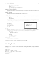
As a result, GLE displays the following message.
GLE version 4.0.13
Usage: gle [options] filename.gle
More information: gle -help
If this message does not appear and you see an error message instead, then GLE is not correctly installed.
Refer to the installation instructions (Appendix A.4) for more information. In the following, we will show
how to construct a simple drawing with GLE.
3
4
CHAPTER 2. TUTORIAL
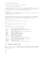
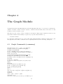
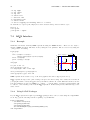
√
(1, 2)
Figure 2.1: Result of your first GLE script.
2.3
Drawing a Line on a Page
Let’s start with drawing a line on the page. GLE needs to know the size of the drawing you whish to
make. This is accomplished with the size command:
size
8 2
This specifies that the output will be 8cm wide and 2cm high. Next we define a “current point” by
moving to somewhere on the page:
amove 0.25 0.25
The origin (0,0) is at the bottom left hand corner of the page. Suppose we wish to draw a line from this
point 5 cm across and 1 cm up:
size 8 2
amove 0.25 0.25
rline 5 1
This is a relative movement as the x and y values are given as distances from the current point, alternatively we could have used absolute coordinates:
size 8 2
amove 0.25 0.25
aline 5.25 1.25
To draw some text on the page at the current point, use the write command:
write "Hi there"
Or, alternatively, you could include arbitrary LaTEX expressions using the tex command:
tex "$(1,\sqrt{2})$"
Now we have constructed complete GLE script, which looks as follows:
size 8 2 box
amove 0.25 0.25
rline 5 1
tex "$(1,\sqrt{2})$"
Enter the above GLE script using a text editor and save it to disk (any editor that saves in UTF8 or ASCII
format will work). The following assumes that you have saved the file under the name “test.gle” in the
folder C:\GLE on Windows, or /home/john/gle on a Unix-like operating system. Now open a command
prompt and go to the folder where you saved the file. Then, run GLE on the file.
On Windows, you do this as follows (C:\> is the prompt):
C:\> cd C:\GLE
C:\GLE> gle test.gle
Or on Unix:
cd ~/gle
gle test.gle
2.4. DRAWING A SIMPLE GRAPH
5
GLE produces by default an Encapsulated PostScript (.eps) file:
GLE 4.0.13 [test.gle]-C-R-[test.eps]
Try viewing the resulting “test.eps” with a PostScript viewer such as GhostView, and compare it to
the output shown in Fig. 2.1. You can also preview it with QGLE, GLE’s graphical user interface. After
you’ve started QGLE, enter the following command at the command prompt.
gle -p test.gle
This will preview the output in the QGLE previewer window. GLE can also create PDF files. This is
accomplished by setting the output device to “pdf”.
gle -device pdf test.gle
Try viewing the resulting “test.pdf” with Acrobat Reader or similar. Other output formats supported
by GLE (eps, ps, pdf, svg, jpg, png, x11) can also be obtained with the -device command line option
(which can be abbreviated to -d). For example, to create a JPEG bitmap file, one can use:
gle -d jpg -r 200 test.gle
Help about the available command line options can be obtained with:
gle -help
and to obtain more information about a particular option, use:
gle -help option
The following command line options are supported by GLE:
-help
-info
-verbosity
-device
-r
-fullpage
-output
-preview
-gs
-version
-compatibility
-calc
-tex
-inc
-texincprefix
-mkinittex
-nocolor
-nomaxpath
2.4
Shows help about command line options
Outputs software version, build date, GLE_TOP, GLE_BIN, etc.
Sets the verbosity level of GLE console output
Selects output device(s)
Sets the resolution for bitmap import/export and PDF output
Selects full page output
Specifies the name of the output file
Previews the output in the QGLE
Call ghostscript for previewing
Selects a GLE version to run
Selects a GLE compatibility mode
Runs GLE in "calculator" mode
Indicates that the script includes LaTeX expressions
Creates an .inc file with LaTeX code
Adds the given subdirectory to the path in the .inc file
Creates "inittex.ini" from "init.tex"
Forces grayscale output
Disables the upper-bound on the drawing path complexity
Drawing a Simple Graph
This section shows how to go about drawing a simple graph. Enter the following data in a new file and
save it as “test.csv”. Note that you can export files in CSV (comma separated values) format with most
spread sheet programs.
1,2
2,6
3,2
4,5
5,9
6
CHAPTER 2. TUTORIAL
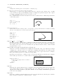
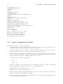
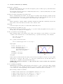
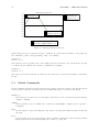
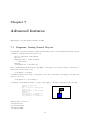
The data is in two columns with a comma separating each column of numbers. The following commands
will draw a simple line graph of the data.
Simple Graph
Output
size 7 4
begin graph
title "Simple Graph"
xtitle "Time"
ytitle "Output"
data
"test.csv"
d1 line marker triangle color red
end graph
9
8
7
6
5
4
3
2
1.0 1.5 2.0 2.5 3.0 3.5 4.0 4.5 5.0
Time
The commands title, xtitle, and ytitle specify the graph title and the axis titles. The command data loads
the data file and the d1 command specifies how the first curve on the graph should look like. These
commands are discussed in detail in Chapter 4. Possible values for the marker option can be found on
the GLE wall reference chart in Appendix A.8.
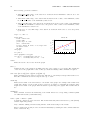
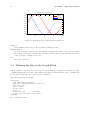
The axis ranges can be specified with xaxis min v0 max v1 and yaxis min v0 max v1 . A smooth line can
be drawn through the data points by changing the d1 command to: d1 line smooth as in the following
example.
Note that the order of the commands is not important, except that circle is a parameter for the option
marker and therefore must come right after it. The same holds for line and smooth and color and blue in
the example “d1 marker circle line smooth color blue”.
Smooth Graph
10
8
Output
size 7 4
begin graph
title "Smooth Graph"
xtitle "Time"
ytitle "Output"
data
"test.csv"
yaxis min 0 max 10
d1 line smooth color red
end graph
6
4
2
0
1.0 1.5 2.0 2.5 3.0 3.5 4.0 4.5 5.0
Time
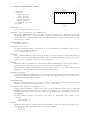
It is simple to change to a bar graph and include last year’s measurements:
Bar Graph
10
8
Output
size 7 4
begin graph
title "Bar Graph"
xtitle "Time"
ytitle "Output"
data
"year-2000.csv"
data
"year-2001.csv"
yaxis min 0 max 10
bar d1,d2 fill red,blue
end graph
6
4
2
0
1
2
3
4
5
Time
Adding min and max values on the axis commands is highly recommended because by default GLE won’t
start from the origin unless the data happens to be very close to zero. It is also difficult to compare
graphs unless they all have the same axis ranges. More information about the graph module is available
in Chapter 4.
Chapter 3
Primitives
A GLE command is a sequence of keywords and values separated by white space (one or more spaces
or tabs). Each command must begin on a new line. Keywords may not be abbreviated, the case is not
significant. All coordinates are expressed in centimetres from the bottom left corner of the page.
GLE uses the concept of a current point which most commands use. For example, the command aline
2 3 will draw a line from the current point to the coordinates (2,3).
The current graphics state also includes other settings like line width, colour, font, 2d transformation
matrix. All of these can be set with various GLE commands.
3.1
Graphics Primitives (a summary)
! comment
@xxx
aline x y [arrow start] [arrow end] [arrow both] [curve α1 α2 d1 d2]
amove x y
arc radius a1 a2 [arrow end] [arrow start] [arrow both]
arcto x1 y1 x2 y2 rad
begin box [fill pattern] [add gap] [nobox] [name xyz] [round val]
begin clip
begin name
begin origin
begin path [stroke] [fill pattern] [clip]
begin rotate angle
begin scale x y
begin table
begin tex
begin text [width exp]
begin translate x y
bezier x1 y1 x2 y2 x3 y3
bitmap filename width height [type type]
bitmap info filename width height [type type]
box x y [justify jtype] [fill color] [name xxx] [nobox] [round val]
circle radius [fill pattern]
closepath
curve ix iy [x1 y1 x y x y ... xn yn]ex ey
define marker markername subroutine-name
ellipse dx dy [options]
7
8
CHAPTER 3. PRIMITIVES
elliptical arc dx dy theta1 theta2 [options]
for var = exp1 to exp2 [step exp3] command [...] next var
grestore
gsave
if exp then command [...] else command [...] end if
include filename
join object1.just sep object2.just [curve α1 α2 d1 d2]
margins top bottom left right
marker marker-name [scale-factor]
orientation o
papersize size
postscript filename.eps width-exp height-exp
print string$ . . .
psbbtweak
pscomment exp
rbezier x1 y1 x2 y2 x3 y3
return exp
reverse
rline x y [arrow end] [arrow start] [arrow both] [curve α1 α2 d1 d2]
rmove x y
save objectname
set arrowangle angle
set arrowsize size
set cap butt — round — square
set color col
set dashlen dashlen-exp
set fill fill color/pattern
set font font-name
set fontlwidth line-width
set hei character-size
set join mitre — round — bevel
set just left — center — right — tl — etc...
set lstyle line-style
set lwidth line-width
set pattern fill pattern
sub sub-name paramter1 paramter2 etc
tex string [name xxx] [add val]
text unquoted-text-string
write string$ . . .
3.2
Graphics Primitives (in detail)
! comment
Indicates the start of a comment. GLE ignores everything from the exclamation point to the end
of the line. This works both in GLE scripts and in data files used in, e.g., graph blocks.
@xxx
Executes subroutine xxx.
aline x y [arrow start] [arrow end] [arrow both] [curve α1 α2 d1 d2]
Draws a line from the current point to the absolute coordinates (x,y), which then becomes the new
current point. The arrow qualifiers are optional, they draw arrows at the start or end of the line,
the size of the arrow is proportional to the current font height.
If the curve option is given, then a Bezier curve is drawn instead of a line. The first control point
is located at a distance d1 and angle α1 from the current point and the second control point is
located at distance d2 and angle α2 from (x,y).
3.2. GRAPHICS PRIMITIVES (IN DETAIL)
9
amove x y
Changes the current point to the absolute coordinates (x,y).
arc radius a1 a2 [arrow end] [arrow start] [arrow both]
Draws an arc of a circle in the anti-clockwise direction, centered at the current point, of radius
radius, starting at angle a1 and finishing at angle a2. Angles are specified in degrees. Zero degrees
is at three o’clock and Ninety degrees is at twelve o’clock.
arc 1.2 20 45
The command narc is identical but draws the arc in the clockwise direction. This is important when
constructing a path.
amove .5 .5
rline 1 .5 arrow end
arc 1 10 160
arc .5 -90 0
arcto x1 y1 x2 y2 rad
Draws a line from the current point to (x1,y1) then to (x2,y2) but fits an arc of radius rad joining
the two vectors instead of a vertex at the point (x1,y1).
amove 1.5 .5
rline 1 0
set lwidth .1
arcto 2 0 -1 1 .5
set lwidth 0
rline -1 1
begin block name ... end block name
There are several block structured commands in GLE. Each begin must have a matching end.
Blocks which change the current graphics state (e.g. scale, rotate, clip etc) will restore whatever
they change at the end of the block. Indentation is optional but should be used to make the GLE
program easier to read.
begin box [fill pattern] [add gap] [nobox] [name xyz] [round val]
Draws a box around everything between begin box and end box. The option add adds a margin
of margin cm to each side of the box to make the box slightly larger than the area defined by the
graphics primitives in the begin box . . . end box group (to leave a gap around text for example).
The option nobox stops the box outline from being drawn.
The name option saves the coordinates of the box for later use with among others the join command.
If the round option is used, a box with rounded corners will be drawn.
begin box add 0.2
begin box fill gray10 add 0.2 round .3
text John
end box
end box
John
begin clip
This saves the current clipping region. A clipping region is an arbitrary path made from lines and
curves which defines the area on which drawing can occur. This is used to undo the effect of a
clipping region defined with the begin path command. See the example CLIP.GLE in appendix B
at the end of the manual.
begin name
Saves the coordinates of what is inside the block for later use with among others the join command.
This command is equivalent to ‘begin box name . . . nobox’.
10
CHAPTER 3. PRIMITIVES
begin origin
This makes the current point the origin. This is good for subroutines or something which has been
drawn using amove,aline. Everything between the begin origin and end origin can be moved as one
unit. The current point is also saved and restored.
begin path [stroke] [fill pattern] [clip]
Initialises the drawing of a filled shape. All the lines and curves generated until the next end path
command will be stored and then used to draw the shape. stroke draws the outline of the shape,
fill paints the inside of the shape in the given colour and clip defines the shape as a clipping region
for all future drawing. Clipping and filling will only work on PostScript devices.
begin rotate 90
text This is
end rotate
This is
begin rotate angle
The coordinate system is rotated anti-clockwise about the current point by the angle angle (in
degrees). For example, to draw a line of text running vertically up the page (as a Y axis label, say),
type:
begin scale x y
Everything between the begin and end is scaled by the factors x and y. E.g., scale 2 3 would make
the picture twice as wide and three times higher.
begin scale 3 1
begin rotate 30
text This is
end rotate
end scale
is
h
is
T
begin table
This module is an alternative to the TEXT module. It reads the spaces and tabs in the source file
and aligns the words accordingly. A single space between two words is treated as a real space, not
an alignment space.
With a proportionally spaced font columns will line up on the left hand side but not on the right
hand side. However with a fixed pitch font, like tt, everything will line up.
begin table
Here is my table
of text see how
22
44
55 33
0.1 999
1
.2
3
33
2
33
it lines up
end table
Here is my table
of text see
how
22 44 55 33
0.1 999 1 .2
3 33 2 33
it lines up
begin text [width exp]
This module displays multiple lines/paragraphs of text. The block of text is justified according to
the current justify setting. See the set just command for a description of justification settings.
If a width is specified the text is wrapped and justified to the given width. If a width is not given,
each line of text is drawn as it appears in the file. Remember that GLE treats text in the same way
that LaTEX does, so multiple spaces are ignored and some characters have special meaning. E.g,
\ ^ _ & { }
To include Greek characters in the middle of text use a backslash followed by the name of the
character. E.g., 3.3\Omega S would produce “3.3ΩS”.
3.2. GRAPHICS PRIMITIVES (IN DETAIL)
11
To put a space between the Omega and the S add a backslash space at the end. E.g., 3.3\Omega\ S
produces “3.3Ω S”
Sometimes the space control characters (e.g. \:) are also ignored, this may happen at the beginning
of a line of text. In this case use the control sequence \glass which will trick GLE into thinking it
isn’t at the beginning of a line. E.g.,
text \glass \:\: Indented text
set hei 0.25 just tl font tt
begin text width 5
This is my paragraph of text to see
if it wraps things at four cm as I have
told it to do.
end text
...
begin text
Now some text without
a width
specified
end text
This is my paragraph of text to
see if it wraps things at four cm
as
I
have
told
it
to
do.
Now some text
without a width
specified
There are several LaTEX like commands which can be used within text. The complete list can be
found in Appendix A.3. A few examples are:
\ \’ \v \u \= \^ \. \H \~ \’’ Implemented TeX accents
^{} _{}
Superscript, subscript
\\ \_
Forced Newline, underscore character
\, \: \;
0.5em, 1em, 2em space (em = width of the letter ‘m’)
\tex{expression}
Any LaTeX expression
\char{22}
Any character in current font
\glass
Makes move/space work on beginning of line
\rule{2}{4}
Draws a filled in box, 2cm by 4cm
\setfont{rmb}
Sets the current text font
\sethei{0.3}
Sets the font height (in cm)
\setstretch{2}
Scales the quantity of glue between words
\lineskip{0.1}
Sets the default distance between lines of text
\linegap{-1}
Sets the minimum required gap between lines
{\rm ...}, {\it ...}
Sets roman, and italic font
{\bf ...}, {\tt ...}
Sets bold, and typewriter (monospaced) font
\alpha, \beta, ...
Greek symbols
begin translate x y
Everything between the begin and end is moved x units to the right and y units up.
bezier x1 y1 x2 y2 x3 y3
Draws a Bézier cubic section from the current point to the point (x3,y3) with Bézier cubic control
points at the coordinates (x1,y1) and (x2,y2). For a full explanation of Bézier curves see the
PostScript Language Reference Manual.
bitmap filename width height [type type]
Imports the bitmap filename. The bitmap is scaled to width×height. If one of these is zero, it is
computed based on the other one and the aspect ratio of the bitmap. GLE supports TIFF, JPEG,
PNG and GIF bitmaps (depending on the compilation options).
Bitmaps are compressed automatically by GLE using either the LZW or the JPEG compression
scheme.
bitmap info filename width height [type type]
Returns the dimensions in pixels of the bitmap in the output parameters width and height.
box x y [justify jtype] [fill color] [name xxx] [nobox] [round val]
Draws a box, of width x and height y, with its bottom left corner at the current point. If the justify
option is used, the box will be positioned relative to the specified point. E.g., TL = top left, CC
= center center, BL = bottom left, CENTER = bottom center, RIGHT = bottom right, LEFT =
bottom left. See set just for a description of justification settings.
If a fill pattern is specified, the box will be filled. Remember that white fill is different from no fill
pattern - white fill will erase anything that was inside the box.
12
CHAPTER 3. PRIMITIVES
If the round option is used, a box with rounded corners will be drawn.
circle radius [fill pattern]
Draws a circle at the current point, with radius radius. If a fill pattern is specified the circle will
be filled.
closepath
Joins the beginning of a line to the end of a line. I.e., it does an aline to the end of the last amove.
curve ix iy [x1 y1 x y x y ... xn yn]ex ey
Draws a curve starting at the current point and passing through the points (x1,y1) . . . (xn,yn),
with an initial slope of (ix,iy) to (x1,y1) and a final slope of (ex,ey). All the vectors are relative
movements from the vector before.
amove
curve
amove
curve
1 1
1 0 0 1 1 0 0 -1 1 0
3.6 1
0 1 0 1 1 0 0 -1 0 -1
margins top bottom left right
This command can be used to define the page margins. Margins are only relevant for making
full-page figures (using the -fullpage command line option). See also the “papersize command.
define marker markername subroutine-name
This defines a new marker called markername which will call the subroutine subroutine-name whenever it is used. It passes two parameters, the first is the requested size of the marker and the second
is a value from a secondary dataset which can be used to vary size or rotation of a marker for each
point plotted.
To define a character from the postscript ZapDingbats font as a marker you would use, e.g.
sub subnamex size mdata
gsave
set just left font pszd hei size
t$ = "\char{102}"
rmove -twidth(t$)/2 -theight(t$)/2
write t$
grestore
end sub
! save font and x,y
! centers marker
! restores font and x,y
The second parameter can be supplied using the mdata command when drawing a graph, this gives
the marker subroutine a value from another dataset to use to draw the marker. For example the
marker could vary in size, or angle, with every one plotted.
d3 marker myname mdata d4
define markername fontname scale dx dy
This command defines a new marker, from any font, it is automatically centered but can be adjusted
using dx,dy. e.g.
defmarker hand pszd 43 1 0 0
ellipse dx dy [options]
This command draws an ellipse with the diameters dx and dy in the x and y directions, respectively.
The options are the same as the circle command.
elliptical arc dx dy theta1 theta2 [options]
This command is similar to the arc command except that it draws an elliptical arc in the clockwise
direction with the diameters dx and dy in the x and y directions, respectively. theta1 and theta2
are the start and stop angle, respectively. The options are the same as for the arc command.
The command elliptical narc is identical but draws the arc in the clockwise direction. This is
important when constructing a path.
3.2. GRAPHICS PRIMITIVES (IN DETAIL)
13
for var = exp1 to exp2 [step exp3] command [...] next var
The for ... next structure lets you repeat a block of statements a number of times.
GLE sets var equal to exp1 and then repeats the following steps.
• If var is greater than exp2 then GLE commands are skipped until the line after the next
statement.
• The value exp3 is added to var.
• The statements between the for and next statement are executed.
If exp1 is greater than exp2 then the loop is not executed.
for x = 1 to 4 step 0.5
amove x 1
aline 5-x 2
next x
grestore
Restores the most recently saved graphics state. This is the simplest way to restore complicated
transformations such as rotations and translations. It must be paired with a previous gsave command.
gsave
Saves the current graphics transformation matrix and the current point and the current colour, font
etc.
if expression then command [...] else command [...] end if
If expression evaluates to true, then execution continues with the statements up to the corresponding
else, otherwise the statements following the else and up to the corresponding end if are executed.
amove 3 3
if xpos()=3 then
text We are at x=3
else
text We are elsewhere
end if
Note: end if is not spelt endif.
include filename
Includes the GLE script “filename” into the current script. This is useful for including library scripts
with subroutines. GLE searches a number of predefined directories for include files. By default,
this includes the current directory and the “lib” or “gleinc” subdirectory of the root directory
(GLE TOP) of your GLE installation. The latter includes a number of subroutine files that are
distributed with GLE (Table 3.1). Additional include directories can be defined by means of the
environment variable GLE USRLIB.
join object1.just sep object2.just [curve α1 α2 d1 d2]
Draws a line between two named objects. An object is simply a point or a box which was given a
name when it was drawn.
The justify qualifiers are the standard GLE justification abbreviations (e.g., TL=top left, see set
just for details)
If sep is written as -, a line is drawn between the named objects e.g.
join fred.tr - mary.tl
Arrow heads can be included at both ends of the line by writing sep as <->. Single arrow heads
are produced by <- and ->. Note that sep must be separated from object1.just and object2.just by
white space.
If the justification qualifiers are omitted, a line will be drawn between the centers of the two objects
(clipped at the edges of the rectangles which define the objects).
14
CHAPTER 3. PRIMITIVES
Table
barstyles.gle
color.gle
colors-gle-4.0.12.gle
contour.gle
electronics.gle
ellipse.gle
feyn.gle
graphutil.gle
piesub.gle
polarplot.gle
shape.gle
simpletree.gle
stm.gle
ziptext.gle
3.1: Include files distributed with GLE.
Defines additional styles for bar plots.
Defines functions for working with colors.
Redefines all colors defined in GLE 4.0.12 and before.
Subroutines for drawing contour plots
Subroutines for drawing electronical cirquits
Draw text in an ellipse
Subroutines for drawing Feynmann diagrams
Subroutines for drawing graphs
Pie chart routines
Polar plotting routines
Drawing various shapes
Draw simple trees
Add labels to images
Draw zipped text
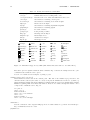
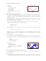
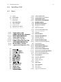
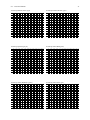
triangle
fcircle
odot
wtriangle
diamond
ominus
ftriangle
wdiamond
oplus
square
fdiamond
otimes
wsquare
cross
star
fsquare
plus
circle
minus
wcircle
asterisk
✥ star2
✯ star3
❂ star4
❀ flower
♣ club
✍ handpen
heart
✉ letter
☎ phone
♠ spade
✈ plane
dag
❍ scircle
ddag
❏ ssquare
.
snake
trianglez
dot
diamondz
Figure 3.1: All markers supported by GLE. (The names that start with “w” are white filled.)
The curve option is explained with the aline command. Fig. 3.3 shows an example where the “join”
command is used with the curve option.
Section 7.1 contains several examples of joining objects.
marker marker-name [scale-factor]
Draws marker marker-name at the current point. The size of the marker is proportional to the
current font size, scaled by the value of scale-factor if present. Markers are referred to by name, eg.
square, diamond, triangle and fcircle. Markers beginning with the letter f are usually filled variants.
Markers beginning with w are filled with white so lines are not visible through the marker. For a
complete list of markers refer to Fig. 3.1.
set just lc
amove 0.5 2.5
marker diamond 1
rmove 0.6 0; text Diamond
amove 0.5 2
marker triangle 1
rmove 0.6 0; text Triangle
...
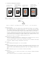
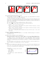
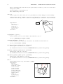
orientation o
Sets the orientation of the output in full-page mode. Possible values are “portrait” and “landscape”.
Fig. 3.2 illustrates these two cases.
papersize size
3.2. GRAPHICS PRIMITIVES (IN DETAIL)
10 cm
21 cm
21 cm
21 cm
29.7 cm
29.7 cm
10 cm
29.7 cm
10 cm
papersize a4paper
orientation landscape
margins 2 2 2 2
papersize a4paper
margins 2 2 2 2
29.7 cm
papersize a4paper
orientation landscape
size 10 10
papersize a4paper
size 10 10
10 cm
15
21 cm
Figure 3.2: Result of different combinations of the commands “papersize”, “margins”, “size”, and “orientation” for fullpage graphics (gle -fullpage figure.gle).
GLE
test.gle
Figure 3.3: Joining two objects using the curve option: “join b1.rc − > b2.tc curve 0 90 1.2 1”.
papersize width height
Sets the paper size of the output. This is used only when GLE is run with the option “-fullpage”.
The command either takes one argument, which should be one of the predefined paper size names
or two numbers, which give the width and height of the output measured in cm. The following
paper sizes are known by GLE: a0paper, a1paper, a2paper, a3paper, a4paper, and letterpaper.
If a “size” command is given in the script, then the output is drawn centered on the page. If no size
command is included in the script, then the output will appear relative to the bottom-left corner of
the page, offset by the page margins (see “margins” command). Fig. 3.2 illustrates these two cases.
The paper size can also be set in GLE’s configuration file (Section 7.5).
postscript filename.eps width-exp height-exp
Includes an encapsulated postscript file into a GLE picture, the postscript picture will be scaled up
or down to fit the width given. On the screen you will just see a rectangle.
Only the width-exp is used to scale the picture so that the aspect ratio is maintained. The height
is only used to display a rectangle of the right size on the screen.
print string$ . . .
This command prints its argument to the console (terminal).
psbbtweak
Changes the default behavior of the bounding box. The default behavior is to have the lower corner
at (-1,-1), which for some interpreters (i.e., Photoshop) will leave a black line around the bottom
and left borders. If this command is specified then the origin of the bounding box will be set to
(0,0).
This command must appear before the first size command in the GLE file.
pscomment exp
Allows inclusion of exp as a comment in the preamble of the postscript file. Multiple pscomment
commands are allowed.
This command must appear before the first size command in the GLE file.
16
CHAPTER 3. PRIMITIVES
rbezier x1 y1 x2 y2 x3 y3
This command is identical to the BEZIER command except that the points are all relative to the
current point.
amove
rbezier
amove
rbezier
0.5
1
0.2
1
2.8
1
2 -1 3
1
0.2
1
2 1.2 1.8 0
return exp
The return command is used inside subroutines to return a value.
reverse
Reverses the direction of the current path. This is used when filling multiple paths in order that
the Non-Zero Winding Rule will know which part of the path is ‘inside’.
With the Non-Zero Winding Rule an imaginary line is drawn through the object. Every time a
line of the object crosses it from left to right, one is added to the counter; every time a line of the
object crosses it from right to left, one is subtracted from the counter. Everywhere the counter is
non-zero is considered to be the ‘inside’ of the drawing and is filled.
0
1
0
1
0
0
1
2
1
0
rline x y [arrow end] [arrow start] [arrow both] [curve α1 α2 d1 d2]
Draws a line from the current point to the relative coordinates (x,y), which then become the new
current point. If the current point is (5,5) then rline 3 -2 is equivalent to aline 8 3. The optional
qualifiers on the end of the command will draw arrows at one or both ends of the line, the size of
the arrow head is proportional to the current font size.
The curve option is explained with the aline command.
rmove x y
Changes the current point to the relative coordinate (x,y). If the current point is (5,5) then rmove
3 -2 is equivalent to amove 8 3.
save objectname
This command saves a point for later use with the join command.
set arrowangle angle
Sets the opening angle of the arrow tips. (Actually, half of the opening angle.)
set arrowsize size
Sets the size of the arrow tips.
set cap butt — round — square
Defines what happens at the end of a wide line.
3.2. GRAPHICS PRIMITIVES (IN DETAIL)
17
set color black
set color white
set color gray50
set
set
set
set
set color 0.3
color
color
color
color
red
#ADFF2F
rgb255(255,140,0)
rgb(0.5,0.2,0.2)
Figure 3.4: Examples of setting the drawing color.
GRID
GRID1
GRID2
GRID3
GRID4
GRID5
SHADE
SHADE1
SHADE2
SHADE3
SHADE4
SHADE5
RSHADE
RSHADE1
RSHADE2
RSHADE3
RSHADE4
RSHADE5
Figure 3.5: Patterns for painting shapes.
set cap butt
set cap round
set cap square
set color col
Sets the current colour for all future drawing operations. GLE supports all SVG/X11 standard
color names. These are listed in Appendix A.7, and include the following: black, white, red, green,
blue, cyan, magenta, yellow, gray10, gray20, . . ., gray90. It is also possible to specify a gray scale as
a real number with 0.0 = black and 1.0 = white. Colors can also be set using the HTML notation,
e.g., #FF0000 = red. Finally, the functions rgb(red,green,blue) and rgb255(red,green,blue) may be
used to create custom colors. Fig. 3.4 gives some examples.
mm$ = "blue"
amove 0.5 0.5
for c = 0 to 1 step 0.05
box 0.2 2 fill (c) nobox
rmove 0.2 0
next c
amove 2 1
box 2 1 fill white nobox
rmove -0.2 0.2
box 2 1 fill mm$
set dashlen dashlen-exp
Sets the length of the smallest dash used for the line styles. This command MUST come before the
set lstyle command. This may be needed when scaling a drawing by a large factor.
set fill fill color/pattern
Sets the color or pattern for filling shapes. This command works in combination with shapes such
as circles, ellipses, and boxes. If the argument is a color, then shapes are filled with the given color
(see “set color). If it is a pattern, then the shapes are painted with the given pattern in black ink.
Fig. 3.5 lists a number of pre-defined patterns. To paint a shape in a color different from black,
first set the color, then the pattern. That is,
18
CHAPTER 3. PRIMITIVES
set fill red
set pattern shade
box 2 2
will draw a box and paint is using the shade pattern and red ink. To draw shapes that are not
filled, use the command “set fill clear”. That is,
set fill clear
box 2 2
will draw an empty box.
set font font-name
Sets the current font to font-name. Valid font-names are listed in Appendix A.2.
There are three types of font: PostScript, LaTEX and Plotter. They will all work on any device,
however LaTEX fonts are drawn in outline on a plotter, and so may not look very nice. PostScript
fonts will be emulated by LaTEX fonts on non-PostScript printers.
set fontlwidth line-width
This sets the width of lines to be used to draw the stroked (Plotter fonts) on a PostScript printer.
This has a great effect on their appearance.
set font pltr
amove .2 .2
text Tester
set fontlwidth .1
set cap round
rmove 0 1.5
text Tester
set hei character-size
Sets the height of text. For historical reasons, concerning lead type and printing conventions, a
height of 10cm actually results in capital letters about 6.5cm tall.
The default value of “hei” is 0.3633 (to mimic the default height of LaTEX expressions).
set join mitre — round — bevel
Defines how two wide lines will be joined together. With mitre, the outside edges of the join are
extended to a point and then chopped off at a certain distance from the intersection of the two
lines. With round, a curve is drawn between the outside edges.
join mitre
join round
join bevel
set just left — center — right — tl — etc...
Sets the justification which will be used for text commands.
amove 0.5 3
set just left
box 1.5 0.6
text Justify left
rmove 2 0
set just bl
box 1.5 0.6
text Justify bl
Justify bl
Justify left
tl
tc
tr
lc
cc
rc
bl
bc
br
3.2. GRAPHICS PRIMITIVES (IN DETAIL)
19
set lstyle line-style
Sets the current line style to line style number line-style. There are 9 predefined line styles (1–9).
When a line style is given with more than one digit the first digit is read as a run length in black,
the second a run length in white, the third a run length in black, etc.
set just left
for z = 0 to 4
set lstyle z
rline 2 0
rmove 0.1 0
write z
rmove -2.1 -0.4
next z
0
1
2
3
4
5
6
7
8
9
9229
set lwidth line-width
Sets the width of lines to line-width cm. A value of zero will result in the device default of about
0.02 cm, so a lwidth of .0001 gives a thinner line than an lwidth of 0.
set pattern fill pattern
Specifies the filling pattern. A number of pre-defined patterns is listed in Fig. 3.5. See the description
of “set fill” for more information.
sub sub-name parameter1 parameter2 etc.
Defines a subroutine. The end of the subroutine is denoted with end sub. Subroutines must be
defined before they are used.
Subroutines can be called inside any GLE expression, and can also return values. The parameters
of a subroutine become local variables. Subroutines are reentrant.
sub tree x y a$
amove x y
rline 0 1
write a$
return x/y
end sub
tree 2 4 "mytree"
slope = tree(2,4,"mytree")
(Normal call to subroutine)
(Using subroutine in an expression)
tex string [name xxx] [add val]
Draw a LaTEX expression at the current point using the current value of ‘justify’. See Section 7.2
for more information. Using the name option, the LaTEX expression can be named, just like a box.
The size of the virtual named box can be increased with the add option.
text unquoted-text-string
This is the simplest command for drawing text. The current point is unmodified after the text is
drawn so following one text command with another will result in the second line of text being drawn
on top of the first. To generate multiple lines of text, use the begin text . . . end text construct.
text "Hi, how’s tricks", said Jack!
write string$ . . .
This command is similar to text except that it expects a quoted string, string variable, or string
expression as a parameter. If write has more than one parameter, it will concatenate the values of
all the parameters.
a$ = "Hello there "
xx = sqrt(10)
t$ = time$()
c$ = a$+t$
write a$+t$ xx
Hello there 23:05:37 3.16228
The built in functions sqrt() and time$() are described in Appendix A.2.
20
CHAPTER 3. PRIMITIVES
Chapter 4
The Graph Module
A graph should start with begin graph and end with end graph. The data to be plotted are organised into
datasets. A dataset consists of a series of (X,Y) coordinates, and has a name based on the letter “d” and
a number between 1 and 99, eg. d1
The name dn can be used to define a default for all datasets. Many graph commands described below
start with dn. This would normally be replaced by a specific dataset number e.g.,
d3 marker diamond
For each xaxis command there is a corresponding yaxis, y2axis and x2axis command for setting the top left
and right hand axes. These commands are not explicitly mentioned in the following descriptions.
4.1
Graph Commands (a summary)
data filename [d1 d2 d3 ...] [d1=c1,c3] [ignore n]
dn bigfile ”all.dat,xc,yc” [marker mname] [line]
dn bigfile xxx$ [autoscale]
dn err d5 errwidth width-exp errup nn% errdown d4
dn herr d5 herrwidth width-exp herrleft nn% errright d4
dn key ”Dataset title”
dn line [impulses] [steps] [fsteps] [hist] [svg smooth]
dn lstyle line-style lwidth line-width color col
dn marker marker-name [msize marker-size] [mdata dn]
dn nomiss
dn smooth — smoothm
dn xmin x-low xmax x-high ymin y-low ymax y-high
fullsize
hscale exp
key pos tl nobox hei exp offset xexp yexp
let ds = exp [from low to high step exp]
let dn = [routine] dm [options]
nobox
size x y
title ”title” [hei ch-hei] [color col] [font font] [dist cm]
vscale exp
x2labels on
xaxis — yaxis — x2axis — y2axis
xaxis base exp-cm
xaxis color col font font-name hei exp-cm lwidth exp-cm
21
22
CHAPTER 4. THE GRAPH MODULE
xaxis dsubticks sub-distance
xaxis format format-string
xaxis grid
xaxis log
xaxis min low max high
xaxis nofirst nolast
xaxis nticks number dticks distance dsubticks distance
xaxis off
xaxis shift cm-exp
xlabels font font-name hei char-hei color col
xnames ”name” ”name” ...
xplaces pos1 pos2 pos3 ...
xside color col lwidth line-width off
xsubticks lstyle num lwidth exp length exp off
xticks lstyle num lwidth exp length exp off
xtitle ”title” [hei ch-hei] [color col] [font font] [dist cm]
y2title ”text-string” [rotate]
yaxis negate
bar dx,... dist spacing
bar dx,... from dy,...
bar dn,... width xunits,... fill col,... color col,...
fill x1,d3 color green xmin val xmax val
fill d4,x2 color blue ymin val ymax val
fill d3,d4 color green xmin val xmax val
fill d4 color green xmin val xmax val
4.2
Graph Commands (in detail)
data filename [d1 d2 d3 ...] [d1=c1,c3] [ignore n]
Specifies the name of a file to read data from. By default, the data will be read into the next free
datasets unless the optional specific dataset names are specified.
A dataset consists of a series of (X,Y) coordinates, and has a name based on the letter d and a
number between 1 and 99, e.g. d1 or d4. Up to 99 datasets may be defined.
From a file with 3 columns the command ‘data "xx.dat"’ would read the first and second columns
as the x and y values for dataset 1 (d1) and the first and third columns as the x and y values for
dataset 2 (d2). The next data command would use dataset 3 (d3).
A data file for two datasets looks like this:
1
2
3
4
2.7
5
7.8
9
3
*
7
4
The first coordinate of dataset d1 would then be (1,2.7) and the first coordinate of dataset d2
would be (1,3). The data values can be space, tab or comma separated.
Missing values can be indicated with “*”, “?”, “-”, or “.”.
Comments can be included with the symbol “!”.
The option d3=c2,c3 allows particular columns of data to be read into a dataset, d3 would read x
values from column 2 and y values from column 3.
The option ignore n makes GLE ignore the first n lines of the data file. This is useful if the first n
lines contain attribute names/types.
4.2. GRAPH COMMANDS (IN DETAIL)
Simple Graph
Output
size 7 3.5
begin graph
size
6 3
title "Simple Graph"
xtitle "Time"
ytitle "Output"
data
"tut.dat"
d1 line marker triangle color red
end graph
23
9
8
7
6
5
4
3
2
1.0 1.5 2.0 2.5 3.0 3.5 4.0 4.5 5.0
Time
dn bigfile ”all.dat,xc,yc” [marker mname] [line]
The bigfile option allows a dataset to be read as it is drawn, (rather than being complete read into
memory before it is drawn) this means that very large datasets can be drawn on a PC without
running out of memory. The axis minimum and maximum must be specified (using the command
xaxis min exp max exp.
By default the first two columns of the data file will be read in, but other columns may be specified.
E.g., all.dat,3,2 would read x values from column 3 and y values from column 2. Or, to read the
4th dataset, specify the file as all.dat,1,5
If the x column is specified as ’0’ then GLE will generate the x data points. E.g., 1,2,3,4,5...
Bigfile also accepts variables in place of the file name, e.g.
xxx$ = "test.dat,2,3"
d1 bigfile xxx$
The AUTOSCALE option pre-reads the file to scale the axis, which is slow but sometimes required,
e.g.:
d1 bifile a.dat line autoscale
Many (but not all) of the normal dn commands can be used with the bigfile command. E.g., marker,
lstyle, xmin, xmax, ymin, ymax, color and lwidth. You cannot use commands like let or bar with the
bigfile command.
dn err d5 errwidth width-exp dn errup nn% errdown d4
For drawing error bars on a graph. The error bars can be specified as an absolute value, as a
percentage of the y value, or as a dataset. The up and down error bars can be specified separately
e.g.,
d3
d3
d3
d3
err .1
err 10%
errup 10% errdown d2
err d1 errwidth .2
Error Bars
begin graph
title "Error Bars"
dn lstyle 2 msize 1.5
d1 marker circle errup 30% errdown 1
d2 marker square err
30% errwidth .1
end graph
30
20
10
0
0
1
2
3
4
5
6
7
8
9 10
dn herr d5 herrwidth width-exp dn herrleft nn% errright d4
These commands are identical to the error bar commands above except that they will draw bars in
the horizontal plane.
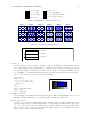
dn key ”Dataset title”
If a dataset is given a title like this a key will be drawn. Use the key command (below, after hscale)
to set the size and position of the key. Use the key module (Chapter 4) to draw more complex keys.
24
CHAPTER 4. THE GRAPH MODULE
100
‘d1 line impulses’
‘d1 line steps’
100
‘d1 line fsteps’
100
80
80
80
80
60
60
60
60
40
40
40
40
20
20
20
20
0
0
0
5
10 15 20
0
0
5
10 15 20
‘d1 line hist’
100
0
0
5
10 15 20
0
5
10 15 20
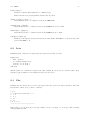
Figure 4.1: The impulses, steps, fsteps, and hist options of the line command.
dn line [impulses] [steps] [fsteps] [hist] [svg smooth]
This tells GLE to draw lines between the points of the dataset. By default GLE will not draw lines
or markers, this is often the reason for a blank graph.
If a dataset has missing values GLE will not draw a line to the next real value, which leaves a gap
in the curve. To avoid this behavior simply use the nomiss qualifier on the dn command used to
define the line. This simply throws away missing values so that lines are drawn from the last real
value to the next real value.
The option svg smooth performs a Savitski Goulay smoothing on the data.
The options impulses, steps, fsteps, and hist draw lines as shown in Figure 4.1.
• impulses: connects each point with the xaxis.
• steps: connects consecutive points with two line segments: the first from (x1,y1) to (x2,y1)
and the second from (x2,y1) to (x2,y2).
• fsteps: connects consecutive points with two line segments: the first from (x1,y1) to (x1,y2)
and the second from (x1,y2) to (x2,y2).
• hist: useful for drawing histograms: assumes that each point is the center of a bin of the
historgram.
dn lstyle line-style lwidth line-width color col
These qualifiers are all fairly self explanatory. See the lstyle command in Chapter 2 for details of
specifying line styles.
dn marker marker-name [msize marker-size] [mdata dn]
Specifies the marker to be used for the dataset. There is a set of pre-defined markers (refer to
Appendix A.1 for a list) which can be specified by name (e.g., circle, square, triangle, diamond, cross,
...). Markers can also be a user-defined subroutine (See the define marker command in Chapter
2). The mdata option allows a secondary dataset to be defined which will be used to pass another
parameter to the marker subroutine, this allows each marker to be drawn at a different angle,size
or colour.
The msize qualifier sets the marker size for that dataset. The size is a character height in cm, so
that the actual size of the markers will be about 0.7 of this value.
dn nomiss
If a dataset has missing values, GLE will not draw a line to the next real value, which leaves a gap
in the curve. To avoid this behavior simply use the nomiss qualifier on the dn command used to
define the line. This simply ignores missing values.
Ignore missing values (nomiss)
10
8
Output
begin graph
title "Ignore missing values (nomiss)"
xtitle "Time"
ytitle "Output"
data
"tut.dat"
d1 lstyle 2
d2 nomiss lstyle 1 marker diamond msize .2
end graph
6
4
2
0
1
2
3
Time
4
5
4.2. GRAPH COMMANDS (IN DETAIL)
25
dn smooth — smoothm
This will make GLE draw a smoothed line through the points. A third degree polynomial is fitted
piecewise to the given points.
The smoothm alternative will work for multi valued functions, i.e., functions which have more than
one y value for each x value.
dn xmin x-low xmax x-high ymin y-low ymax y-high
These commands map the dataset onto the graph’s boundaries. The data will be drawn as if the
X axis was labelled from x-low to x-high (regardless of how the axis is actually labelled). A point
in the dataset at X = x-low will appear on the left hand edge of the graph.
fullsize
This is equivalent to vscale 1, hscale 1, noborder. It makes the graph size command specify the size
and position of the axes instead of the size of the outside border.
hscale exp
Scales the length of the yaxis. See vscale. The default value is 0.7.
key pos tl nobox hei exp offset xexp yexp
This command allows the features of a key to be specified. The pos qualifier sets the position of
the key. E.g., tl=topleft, br=bottomright, etc.
let ds = exp [ from low to high step exp]
This command defines a new dataset as the result of an expression on the variable x over a range
of values. It also allows the use of other datasets. E.g., to generate an average of two datasets:
data "file.csv" d1 d2
let d3 = d1+d2/2
Or to generate data from scratch:
let d1 = sin(x)+log(x) from 1 to 100 step 1
Calculating Formulas
5
4
Output
begin graph
...
let d1 = 1/x from 0.2 to 10
let d2 = sin(x)*2+2 from 0 to 10
let d3 = 10*(1/sqrt(2*pi))*
exp(-2*(sqr(x-4)/sqr(2))))
from 0.2 to 10 step 0.1
dn line
d2 lstyle 2 color red
d3 lstyle 3 color blue
end graph
3
2
1
0
0
1
2
3
4
5
6
7
8
9
Time
If the xaxis is a LOG axis then the step option is read as the number of steps to produce rather
than the size of each step. The “from”, “to”, and “step” parameters are optional. The values of
“from” and “to” default to the horizontal axis’ range.
NOTE: The spacing around the ‘=’ sign and the lack of spaces inside the expression
are necessary.
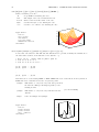
let dn = [routine] dm [options]
GLE includes several fitting routines that allow an equation to be fit to a data series. These routines
can be included in a ‘let’ expression as shown above, where dn will contain results of fitting routine
to the data in dm, and the [options] control the limits to which the data in dn extends.
The following routines are available :
• linfit: fits the data in dm to the straight line equation y = m · x + b.
• logfit: fits the data in dm to the equation y = a · exp(b · x).
• log10fit: fits the data in dm to the equation y = a · 10b·x .
• powxfit: fits the data in dm to the equation y = a · xb .
26
CHAPTER 4. THE GRAPH MODULE
The following options are available :
• limit data x The range of the data in dn extends from the minimum x value in dm to the
maximum x value in dm.
• limit data y The range of the data in dn extends from the x value of the minimum y value
in dm to the x value of the maximum y value in dm.
• limit data The range of the data in dn extends from the greater of the x value of the minimum
y value or the minimum x value in dm to the greater of the x value of the maximum y value
or the maximum x value in dm.
• from xmin to xmax The range of the data in dn extends from the xmin to xmax as specified
by the user.
slope = 0; offs = 0
set just rc
amove xg(xgmax)-0.25 yg(2)
tex "$y = " + format$(slope,"fix 2") +
"x + " + format$(offs,"fix 2") + "$"
Linear fit
10
y = ax + b
begin graph
title "Linear fit"
xtitle "$x$"
ytitle "$y = ax + b$"
data
"fitlin.dat"
let d2 = linfit d1 from 0 to 10 slope offs
d1 marker circle
d2 line
end graph
8
6
4
y = 0.76x + 2.04
2
0
0
2
4
6
8
10
x
nobox
This removes the outer border from the graph.
size x y
Defines the size of the graph in cm. This is the size of the outside box of a graph. The default size
of the axes of the graph will be 70% of this, (see vscale and hscale). This command is required.
title ”title” [hei ch-hei] [color col] [font font] [dist cm]
This command gives the graph a centred title. The list of optional keywords specifies features of it.
The dist command is used for moving the title up or down.
vscale exp
This sets the width of the axis relative to the width of the graph. For example with a 10cm wide
graph and a vscale of .6 the x axis would be 6cm long. A setting of 1.0 makes the xaxis the same
length as the width of the graph, which is useful for positioning some graphs. The default value is
0.7.
x2labels on
This command ‘activates’ the numbering of the x2axis. There is a corresponding command ‘y2axis
on’ which will activate y2axis numbering.
xaxis — yaxis — x2axis — y2axis
A graph is considered to have four axes: The normal xaxis and yaxis as well as the top axis (x2axis)
and the right axis (y2axis).
Any command defining an xaxis setting will also define that setting for the x2axis.
The secondary axes x2 and y2 can be modified individually by starting the axis command with the
name of that axis. E.g.,
4.2. GRAPH COMMANDS (IN DETAIL)
27
X2-axis
10
Y2-axis
8
Y-axis
begin graph
size 6 3
xtitle "X-axis"
ytitle "Y-axis"
x2title "X2-axis"
y2title "Y2-axis"
x2ticks length 0.6
x2subticks color red
end graph
6
4
2
0
0
1
2
3
4
5
6
7
8
9 10
X-axis
xaxis base exp-cm
Scale the axis font and ticks by exp-cm.
xaxis color col font font-name hei exp-cm lwidth exp-cm
These axis qualifiers affect the colour, lstyle, lwidth, and font used for drawing the xaxis (and
the x2axis). These can be overriden with more specific commands. E.g., ‘xticks color blue’ would
override the axis colour when drawing the ticks. The subticks would also be blue as they pick up
tick settings by default.
xaxis dsubticks sub-distance
See xaxis nticks below.
xaxis format format-string
Specifies the number format for the labels. See the documentation of format$ on page 38 for a
description of the syntax. Example:
xaxis format "fix 1"
xaxis grid
This command makes the xaxis ticks long enough to reach the x2axis and the yaxis ticks long
enough to reach the y2axis. When used with both the x and y axes this produces a grid over the
graph. Use the xticks lstyle command to create a faint grid.
xaxis log
Draws the axis in logarithmic style, and scales the data logarithmically to match (on the x2axis or
y2axis it does not affect the data, only the way the ticks and labelling are drawn)
Be aware that a straight line should become curved when drawn on a log graph. This will only
happen if you have enough points or have used the smooth option.
xaxis min low max high
Sets the minimum and maximum values on the xaxis. This will determine both the labelling of the
axis and the default mapping of data onto the graph. To change the mapping see the dataset dn
commands xmin, ymin, xmax, and ymax.
xaxis nofirst nolast
These two switches simply remove the first or last (or both) labels from the graph. This is useful
when the first labels on the x and y axis are too close to each other.
xaxis nticks number dticks distance dsubticks distance
nticks specifies the number of ticks along the axis. dticks specifies the distance between ticks and
dsubticks specifies the distance between subticks. For example, to get one subtick between every
main tick with main ticks 3 units apart, simply specify dsubticks 1.5. Alternatively, one can also
use nsubticks.
By default ticks are drawn on the inside of the graph. To draw them on the outside use the
command:
xticks length -.2
yticks length -.2
xaxis off
Turns the whole axis off — labels, ticks, subticks and line. Often the x2axis and y2axis are not
required, they could be turned off with the following commands:
x2axis off
y2axis off
28
CHAPTER 4. THE GRAPH MODULE
xaxis shift cm-exp
This moves the labelling to the left or right, which is useful when the label refers to the data between
the two values.
xlabels font font-name hei char-hei color col
This command controls the appearance of the axis labels but not the axis title.
xnames ”name” ”name” ...
This command replaces the numeric labelling with absolutely anything. Given data consisting of
seven measurements, taken from Monday to Sunday, one per day then
xnames "Mon" "Tue" "Wed" "Thu" "Fri" "Sat" "Sun"
xaxis min 0 max 6 dticks 1
would give the desired result. Note it is essential to define a specific axis minimum, maximum,
dticks, etc., otherwise the labels may not correspond to the data.
If there isn’t enough room on the line for all the names then simply use an extra xnames command.
Names & Places
20
Happyness
begin graph
ytitle "Happyness"
title "Names \& Places"
xnames "Mon" "Tue" "Wed" "Thu"
xnames "Fri" "Sat" "Sun"
xaxis min 0 max 6 dticks 1
...
end graph
16
12
8
4
0
Mon
Tue
Wed
Thu
Fri
Sat
Sun
xplaces pos1 pos2 pos3 ...
This is similar to the xnames command but it specifies a list of points which should be labelled.
This allows labelling which isn’t equally spaced. For example:
xplaces 1
2
5
7
xnames "Mon" "Tue" "Fri" "Sun"
If there isn’t enough room on the line for all the places then simply use an extra xplaces command.
xside color col lwidth line-width off
This command controls the appearance of the axis line, i.e. the line to which the ticks are attached.
xsubticks lstyle num lwidth exp length exp off
This command gives fine control of the appearance of the axis subticks.
xticks lstyle num lwidth exp length exp off
This command gives fine control of the appearance of the axis ticks. Note: To get ticks on the
outside of the graph, i.e. pointing outwards, specify a negative tick length:
xticks length -.2
yticks length -.2
xtitle ”title” [hei ch-hei] [color col] [font font] [dist cm]
This command gives the axis a centered title. The list of optional keywords specify features of it.
The dist command is used for moving the title up or down.
xaxis negate
This is reversed the numbering on the y axis. For use with measurements below ground, where you
want zero at the top and positive numbers below the zero.
y2title ”text-string” [rotate]
By default the y2title is written vertically upwards. The optional rotate keyword changes this
direction to downwards. The rotate option is specific to the y2title command.
4.3. BAR GRAPHS
4.3
4
10
5
10
Log Yaxis
10
3
2
10
2
1
10
Y2title rotated
begin graph
xaxis min 0 max 9 nofirst nolast
xaxis hei 0.4 nticks 6 dsubticks 0.3
xaxis lwidth 0.05 color red
xticks length 0.2
ytitle "Log Yaxis"
yaxis log min 1 max 10
yticks length 0.2
y2axis min 1 max 10000 format "sci 0 10"
y2side color blue
y2title "Y2title rotated " hei 0.3 rotate
x2axis off
y2labels on
let d1 = sin(x)*4+5 from 0 to 9
dn line color blue
end graph
29
0
1
10
1.5
3.0
4.5
6.0
7.5
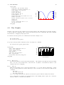
Bar Graphs
Drawing a bar graph is a subcommand of the normal graph module. This allows bar and line graphs to
be mixed. The bar command is quite complex as it allows a great deal of flexibility. The same command
allows stacked, overlapping and grouped bars.
For stacked bars use separate bar commands as in the first example below:
bar d1 fill black
bar d2 from d1 fill gray10
For grouped bars put all the datasets in a list on a single bar command:
bar d1,d2,d3 fill gray10,gray40,black
Bean stalk data
6
Height of stalk
begin graph
title "Bean stalk data" dist 0.1
xtitle "Year measured"
ytitle "Height of stalk"
xaxis dticks 1
yaxis min 0 max 6 dticks 2
data "gc_bean.dat"
bar d1,d2,d3 fill blue,orange,red
end graph
4
2
0
86
87
88
89
90
Year measured
bar dx,... dist spacing
Specifies the distance between bars in dataset(s) dx,.... The distance is measured from the left hand
side of one bar to the left hand side of the next bar. A distance of less than the width of a bar
results in the bars overlapping.
bar dx,... from dy,...
This sets the starting point of each bar in datasets dx,... to be at the value in datasets dy,..., and is
used for creating stacked bar charts. Each layer of the bar chart is created with an additional bar
command.
bar d1,d2
bar d3,d4 from d1,d2
bar d5,d6 from d3,d4
Note 1: It is important that the values in d3 and d4 are greater than the values in d1 and d2.
Note 2: Data files for stacked bar graphs should not have missing values, replace the * character
with the number on its left in the data file.
30
CHAPTER 4. THE GRAPH MODULE
Bean stalk data
begin graph
...
data "gc_bean.dat"
bar d1 fill gray20
bar d2 from d1 fill white
end graph
Height of stalk
5
4
3
2
1
0
86
87
88
89
90
Year measured
bar dn,... width xunits,... fill col,... color col,...
The rest of the bar qualifiers are fairly self explanatory. When several datasets are specified, separate
them with commas (with no spaces between commas).
bar d1,d2 width 0.2 dist 0.2 fill gray10,gray20 color red,green
4.4
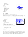
3D Bar Graphs
3d Bar graphs are now supported, the commands are:
bar d1,d2
bar d3,d4
3d .5 .3
3d .5 .3
side red,green notop
side red,green top black,white
Take note of comma’s.
bar dx,... 3d xoffset yoffset side color list top color list [notop]
3d xoffset yoffset
Specifies the x and y vector used to draw the receding lines, they are defined as fractions of the
width of the bar. A negative xoffset will draw the 3d bar on the left side of the bar instead of the
right hand side.
side color list
The color of the side of each of the bars in the group.
top color list
The color of the top part of the bar
notop
Turns off the top part of the bar, use this if you have a stacked bar graph so you only need sides
on the lower parts of each stack.
Bean stalk data
6.0
Height of stalk
begin graph
...
data "gc_bean.dat"
bar d1,d2,d3 dist 0.25 width 0.15 3d 1 0.25 &
fill red,blue,forestgreen &
side orange,dodgerblue,green
end graph
5.0
4.0
3.0
2.0
1.0
0.0
86
87
88
89
Year measured
Note: You won’t see the color of the side or top on the pc screen.
90
4.5. FILLING BETWEEN LINES
4.5
31
Filling Between Lines
fill x1,d3 color green xmin val xmax val
Fills between the xaxis and a dataset, use the optional xmin, xmax, ymin, ymax qualifiers to clip the
filling to a smaller region
fill d4,x2 color blue ymin val ymax val
This command fills from a dataset to the x2axis.
fill d3,d4 color green xmin val xmax val
This command fills between two datasets.
fill d4 color green xmin val xmax val
This command treats the dataset as a polygon and fills it. The dataset should be a closed polygon.
4.6
Shading areas of the graph
6
Year measured
begin graph
title "Shading areas of the graph" dist 0.1
xtitle "Height of stalk"
ytitle "Year measured"
xaxis min 86 max 90
yaxis min 0 max 6
data "gc_fill.dat"
fill d2,x2 color gray40
fill x1,d1 color gray10 xmin 85 xmax 88
fill x1,d1 color gray90 xmin 88 xmax 91
dn line
end graph
5
4
3
2
1
0
86
87
88
89
90
Height of stalk
Notes on Drawing Graphs
4.6.1
Importance of Order
Most of the graph commands can appear in any order, but in some cases order is significant.
As some let commands operate on data which has been read into datasets, the data commands should
precede the let commands.
The wildcard dn command should appear before specific d1 commands which it will override.
By default xaxis commands also change the x2axis, and xlabels commands also change x2labels, so to
specify different settings for the x and x2 axes, put the x2 settings after the x settings.
begin graph
size 10 10
data a.dat
let d2 = d1*3
dn marker square lstyle 3
d2 marker dot
xaxis color green
xticks color blue
x2axis color black
end graph
4.6.2
! sets d1 and d2
Line Width
When scaling a graph up or down for publication the default line width may need changing. To do this
simply specify a set lwidth command before beginning the graph.
32
CHAPTER 4. THE GRAPH MODULE
size 10 10
set lwidth .1
begin graph
...
end graph
Chapter 5
The Key Module
The key module is used for drawing keys. The key can be either specified through a separate key block or
directly in the graph block (by prefixing the key commands with the keyword “key”). This chapter first
discusses how to define the key using a key block. Section 5.3 shows how to include the key commands
directly in a graph block.
The key block usually comes directly after the graph block as follows:
begin graph
...
end graph
begin key
position tr
offset 0.2 0.2
text "Blue"
marker circle
fill blue
text "Red"
marker triangle fill red
lstyle 2
text "Orange" marker square
fill orange lstyle 3
end key
10.0
Blue
Red
Orange
7.5
5.0
2.5
0.0
0.0
2.5
5.0
7.5
10.0
The key block consists of two parts: (a) global commands, and (b) the definitions of the entries. Global
commands appear at the beginning of the key and define, e.g., the position of the key. In the example,
“position” and “offset” are global commands. Multiple global commands are allowed on a given line. The
entry definitions start after the global commands. All comands relevant to a given entry must appear on
the same line. In the example, there are three entry definitions and each definition starts with the “text”
command. Entries can be organized into columns using the “separator” command.
There are two possible ways to set the position of a key: (a) the key can be positioned relative to the
33
34
CHAPTER 5. THE KEY MODULE
Various key positions
1.0
0.9
position tr
offset -0.1 0
position tl
0.8
0.7
0.6
0.5
0.4
0.3
position br
offset 0.25 0.25
0.2
0.1
0.0
0.0
0.1
0.2
0.3
0.4
0.5
0.6
0.7
0.8
0.9
1.0
justify bc
absolute pagewidth()/2 0.1
Figure 5.1: Various positions for the key.
graph, and (b) it can be positioned at given coordinates. To position the key relative to the graph, use
the commands “position” and (optionally) “offset”. For example,
position tr
offset 0.2 0.2
places the key at the top-right corner of the graph 0.2 cm from each side. To position the key at given
coordinates use the “justify” and “absolute” commands. For example,
justify bc
absolute 5 0.1
places the bottom-center of the key at position (5 cm, 0.1 cm). Fig. 5.1 gives some examples of positioning
the key.
5.1
Global Commands
Global commands appear at the start of the key block. They control the position of the key and various
other properties of the key. Several global key commands may appear on one line in the script.
absolute x y
Places the key at position (x, y) on the figure. The anchor point of the key is specified with the
“justify” command.
coldist d
Sets the distance between columns. (To obtain a key with multiple columns, use the “separator”
command.)
dist d
Sets the distance between the different components of an entry (the marker, the line, the fill, and
the text).
hei h
Sets the height of the text in the entries of the key. If this command is not given, then the current
height is used. (To set the current height, use “set hei”, see page 18.)
5.2. ENTRY DEFINITION COMMANDS
35
justify x
Sets the anchor point of the key. Possible values: tl, bl, tr, br, tc, bc, lc, rc, cc. These stand for
top-left, bottom-left, top-right, bottom-right, top-center, bottom-center, left-center, right-center,
and center. Use this command in combination with the “absolute” command. Fig. 5.1 gives some
examples.
llen x
Sets the length of the line in the entries.
lpos x
Sets the vertical position of the line in the entries. (This is normally set automatically.)
margins x y
Sets the margins of the key block. (The space between the border and the entries.)
nobox
Do not draw a border around the key.
offset x y
Specifies the distance in cm between the position specified with the “position” or “pos” command
and the actual key. A negative offset places the key outside of the graph (Fig. 5.1).
position x or pos x
Specifies the position of the key on the graph. Possible values: tl, bl, tr, br, tc, bc, lc, rc, cc. These
stand for top-left, bottom-left, top-right, bottom-right, top-center, bottom-center, left-center, rightcenter, and center. Optionally, the “offset” command can be combined with this command. Fig. 5.1
gives some examples.
base h or row h
Sets the base scale of the entries. The sizes of all components are initialized based on this. E.g., to
change the size of the filled box in an entry, use this command.
5.2
Entry Definition Commands
Each entry in the key is represented by one line in the key block, and all commands for a given entry
must appear on that line. The following commands can be used to define key entries.
color c
Sets the color of the line and marker. The other components of the key are drawn in the default
color. (To set the default color, use “set color”, see page 17.)
fill p
Sets the fill color or pattern.
line
Shorthand for “lstyle 1”.
lstyle s
Sets the line style.
lwidth
Sets the width of the line.
marker m
Sets the marker.
mscale x
Sets the scale of the marker.
msize x
Sets the size of the marker.
36
CHAPTER 5. THE KEY MODULE
Implicitly defined key
1.0
Sine
Cosine
0.8
0.6
0.4
0.2
0.0
-0.2
-0.4
-0.6
-0.8
-1.0
0
/2
3 /2
2
Figure 5.2: Defining the key together with the graph block.
pattern x
Sets the filling pattern. Fig. 3.5 shows examples of filling patterns.
separator [lstyle s]
Use this command to divide the key into multiple columns. If the “lstyle” option is given, then a
line is drawn between the columns in the given style. Possible values are given with the description
of the “set lstyle” command on page 19.
text s
The text for the entry.
5.3
Defining the Key in the Graph Block
It is also possible to define the key in the graph block itself. This is accomplished by prefixing global key
commands with the keyword “key”. The entries are in this case defined with the “dn” commands and
the labels are set with the “key” option to these commands.
The following presents an example:
begin graph
title "Implicitly defined key"
xaxis min 0 max 2*pi dticks pi/2 format "pi"
yaxis min -1 max 1
let d1 = sin(x)
let d2 = cos(x)
key pos tr
d1 line color red
key "Sine"
d2 line color blue lstyle 2 key "Cosine"
end graph
Fig. 5.2 shows the result.
Chapter 6
Programming Facilities
6.1
Expressions
Wherever GLE is expecting a number it can be replaced with an expression. For example
rline 3 2
and
rline 9/3 sqrt(4)
will produce the same result.
An expression in GLE is delimited by white space, so it may not contain any spaces - ‘rline 3*3 2’ is valid
but ‘rline 3 * 3 2’ will not work.
Or ‘let d2 = 3+sin(d1)’ will work and ‘let d2= 3 + sin(d1)’ won’t.
Expressions may contain numbers, arithmetic operators (+, -, *, /, ^ (to the power of)), relational
operators (>, <, =>, <=, =, <>) boolean operators (and, or), variables and built-in functions.
When GLE is expecting a colour or marker name (like ‘green’ or ‘circle’) it can be given a string variable,
or an expression enclosed in braces.
6.2
Functions Inside Expressions
eval(str)
Evaluates the given string as if it was a GLE expression and returns the result. E.g., eval("3+4")
returns 7.
arg(i), arg$(i), nargs()
Provide access to the command line arguments that are passed to GLE. This is useful for generating multiple similar plots from a single script. arg(i) returns the i-the argument (as a number),
arg$(i) returns the i-the argument as a string, and nargs() returns the number of arguments. Only
arguments that come after the name of the GLE script are counted. For example, if GLE is run as:
gle -o graph-1.eps graph.gle "Title" 0.5
then nargs() returns 2, arg$(1) returns “Title”, and arg(2) returns 0.5.
The typical use of these functions is to create a script “graph.gle” as follows:
37
38
CHAPTER 6. PROGRAMMING FACILITIES
size 10 10
begin graph
title arg$(1)
data arg$(2)
d1 line color red
end graph
and then creating different graphs by running GLE multiple times:
gle -o beans.eps graph.gle "Beans" "beans.csv"
gle -o peas.eps graph.gle "Peas" "peas.csv"
This will create two graphs: “beans.eps” and “peas.eps”. The arg() functions can be used at all
places in the script where an expression is expected. They can even be used in place of GLE
commands in a graph block by means of the \expr() function. For example,
data "file.csv"
d\expr{arg(1)} line color red
in the graph block will allow one to draw different data sets from a single file on multiple graphs.
To do so, run:
gle -o d1.eps graph.gle 1
gle -o d2.eps graph.gle 2
format$(exp,format)
Returns a string representation of exp formatted as specified in format.
Basic formats:
• dec, hex [upper—lower], bin: format as decimal, hexadecimal (upper-case or lower-case), or
binary.
• fix places: format with places decimal places.
• sci sig [e,E,10] [expdigits num] [expsign]: format in scientific notation with sig significant digits.
Use ‘e’, ‘E’, or ‘10’ as notation for the exponent. With the option expdigits the number of
digits in the exponent can be set and expsign forces a sign in the exponent.
• round sig: format a number with sig significant digits.
Options for all formats:
• nozeroes: remove unnecessary zeroes at the end of the number.
• sign: also include a sign for positive numbers.
• pad nb [left] [right]: pad the result with spaces from the left or right.
• prefix nb: prefix the number with zeroes so that nb digits are obtained.
• min val: use format for numbers ≥ val.
• max val: use format for numbers ≤ val.
Examples:
• format$(3.1415, “fix 2”) = 3.14
• format$(3756, “round 2”) = 3800
• format$(3756, “sci 2 10 expdigits 2”) = 3.8 · 1003
Several formats can be combined into one string: ”sci 2 10 min 1e2 fix 0” uses scientific notations
for numbers above 102 and decimal notation for smaller numbers.
pagewidth(), pageheight()
These functions return the width and height of the output. These are the values set with the ‘size’
command.
pointx(), pointy()
These functions return the x and y values of a named point.
6.3. USING VARIABLES
39
begin box add 0.1 name mybox
write "Hello"
end box
amove pointx(mybox.bc) pointy(mybox.bc)
rline 0 -2 arrow end
twidth(str), theight(str), tdepth(str)
These functions return the width, depth and height of a string, if it was printed in the current font
and size.
width(obj), height(obj)
These functions return the width and height of a named object.
xend(), yend()
These functions return the end point of the last thing drawn. This is of particular interest when
drawing text.
text abc
set color blue
text def
This would draw the def on top of the abc. To draw the def immediately following the abc simply
do the following (Note that absolute move is used, not relative move):
set just left
text abc
set color gray20
amove xend() yend()
text def
abcdef
xg(), yg()
With these functions it is possible to move to a position on a graph using the graph’s axis units.
To draw a filled box on a graph, at position x=948, y=.004 measured on the graph axis:
begin graph
xaxis min 100 max 2000
yaxis min -.01 max .01
...
end graph
amove xg(948) yg(.004)
box 2 2 fill gray10
xpos(), ypos()
Returns the current x and y points.
See Appendix A.2 for an overview of all functions provided by GLE.
6.3
Using Variables
GLE has two types of variables, floating point and string. String variables always end with a dollar sign.
A string variable contains text like “Hello, this is text”, a floating point variable can only store numbers
like 1234.234.
name$ = "Joe"
height = 6.5
! Height of person
shoe = 0.05
! shoe adds to height of person
amove 1 1
box 0.2 height+shoe
write name$
40
CHAPTER 6. PROGRAMMING FACILITIES
6.4
Programming Loops
The simple way to draw a 6 × 8 grid would be to use a whole mass of line commands:
amove
rline
amove
rline
...
amove
rline
0
0
1
1
0
8
0
8
6 0
6 8
this would be laborious to type in, and would become impossible to manage with several grids. By using
a simple loop this can be avoided:
for x = 0 to 6
amove x 0
rline x 8
next x
for y = 0 to 8
amove 0 y
rline 6 y
next y
To draw lots of grids all of different dimensions a subroutine can be defined and then used again and
again:
sub grid nx ny
begin origin
for x = 0 to nx
amove x 0
aline x ny
next x
for y = 0 to ny
amove 0 y
aline nx y
next y
end origin
end sub
amove
grid
amove
grid
2
6
2
9
4
8
2
5
Now the main GLE file will be much easier to manage if the subroutine definition is moved into a separate
file:
include "griddef.gle"
amove
grid
amove
grid
2
2
2
9
4
4
2
5
More information about the “include” command can be found on page 13.
6.4.1
Default Arguments
Given the following subroutine definition:
6.5. I/O FUNCTIONS
41
sub mysub x y color$ fill$
default color "black"
default fill
"clear"
print "Color: " color$
print "Fill: " fill$
end sub
the following calls are valid:
mysub
mysub
mysub
mysub
mysub
mysub
6.5
1
1
1
1
1
1
0
0
0
0
0
0
red
red green
fill blue
color red
color red fill blue
I/O Functions
The following I/O functions are available:
fopen name file [read|write]
Open the file “name” for reading or for writing. The resulting file handle is stored in variable “file”
and must be passed to all other I/O functions.
fclose file
Close the given file.
fread file x1 . . .
freadln file x1 . . .
Read entries from “file” into given arguments x1 . . .
fwrite file x1 . . .
Write given arguments to “file”.
fwriteln file x1 . . .
Write given arguments to “file” and start a new line.
fgetline file line$
Read an entire line from “file” and store it in the string “line$”.
ftokenizer file commentchar spacetokens singletokens
Sets up the parameters of the tokenizer for “file”.
For example:
fopen "file.dat" f1 read
fopen "file.out" f2 write
until feof(f1)
fread f1 x y z
aline x y
rline x z
fwriteln f2 x*2 "y =" y
next
fclose f1
fclose f2
42
6.6
CHAPTER 6. PROGRAMMING FACILITIES
Device dependend Control
A built in function which returns a string describing the device is available.
e.g. DEVICE$() = "HARDCOPY, PS,"
on the postscript driver.
This can be used to use particular fonts etc on appropriate devices. E.g.:
if pos(device$(),"PS,",1)>0 then
set font psncsb
end if
Chapter 7
Advanced features
This chapter covers the advanced features of GLE.
7.1
Diagrams, Joining Named Objects
To draw lines between boxes which contain text, first name each box as it is drawn and then use the join
command to draw the lines between the boxes.
box 2 3 fill blue name square
amove 5 5
begin box add .1 name titlebox
text Title
end box
join square.tr -> titlebox.bc
These commands draw a line from the “Top Right” of the square to the “Bottom Centre” of the titlebox,
with an arrow at the titlebox end.
join square - titlebox
would draw a line from the centre of the square to the centre of the titlebox but clipped correctly at the
edges of both boxes.
join square.tc <-> titlebox.v
would draw a vertical line from the top centre of the square to the titlebox with arrows at both ends.
set hei .3 font plge
amove 1.2 .2
box 1 1 fill blue name square
amove 1.9 2
begin box add .1 name titlebox
text Title
end box
join square.tr -> titlebox.tr
join square <- titlebox
join square.tc <-> titlebox.v
Named points on each box:
.bl
.bc
.br
.cr
Bottom
Bottom
Bottom
Centre
left
centre
right
right
43
44
.tr
.tc
.tl
.cl
.v
.h
.cc
.ci
CHAPTER 7. ADVANCED FEATURES
Top right
Top centre
Top left
Centre left
Vertical line
Horizontal line
Centre centre
Circle clipping (for drawing lines to a circle)
To draw lines to a given point, simply move there and save that point as a named object.
rmove 2 3
save apoint
join apoint - square
7.2
7.2.1
LaTEX Interface
Example
GLE files can include arbitrary LaTEX expressions using the LaTEX interface. There are two ways to
include a LaTEX expression. The first one is by using the ‘tex’ primitive. The second one is by using the
‘\tex{}’ macro in a string.
set just bc hei 0.6
amove xg(sqrt(5)) yg(2.5)
tex "$\sqrt{5}$" add 0.1 name sq5b
Plot of f (x) =
6
√
4
y = f (x)
begin graph
...
title "\tex{Plot of $f(x) =
\frac{x-\sqrt{5}}{(x-1)\cdot(x-4)}$}"
xtitle "\tex{$x$}"
ytitle "\tex{$y = f(x)$}"
...
end graph
5
2
0
-2
-4
-6
0
amove pointx(sq5b.bc) pointy(sq5b.bc)
aline xg(sqrt(5)) yg(0) arrow end
√
x− 5
(x−1)·(x−4)
1
2
3
4
5
x
LaTEX expressions are drawn on top of all other graphics and cannot clipped (Section 7.3).
LaTEX expressions respect the ‘just’ setting, but ignore the ‘hei’ setting. As a result, the font sizes in
your graphics will be exactly the same as in your main document. To obtain different font sizes, use the
font size primitives provided by LaTEX (e.g., \large, . . .). In the future, a setting ‘scaletexfonts’ will
be added to control scaling of the fonts in LaTEX expression. If this setting is true, GLE will respect the
value of ‘hei’.
7.2.2
Using LaTeX Packages
If your LaTEX expressions require special LaTEX packages, these can be loaded using the texpreamble
block. E.g., put the following near the beginning of your GLE file:
begin texpreamble
\documentclass{llncs}
\usepackage{amsmath}
\usepackage{amssymb}
\DeclareMathSymbol{\R}{\mathbin}{AMSb}{"52}
end texpreamble
7.3. FILLING, STROKING AND CLIPPING PATHS
7.2.3
45
Import in a TeX Document
There are two methods for importing the output of a GLE file with TEX expressions in your LaTEX
document. The most obvious one is by just importing the .eps/.pdf file generated by GLE with
\includegraphics.
An alternative method is by using GLS’s command line option -inc. If this option is supplied, then GLE
will create besides the usual .eps or .pdf file also an .inc file. This .inc file can be imported in a LaTEX
document as follows.
\input{myfile.inc}
The .inc file tells latex (or pdflatex) to include the .eps/.pdf output file created by GLE. It also
includes TEX draw commands for drawing the LaTEX expressions on top of the GLE output. Note that
the .eps/.pdf file created by GLE does not include these if -inc is used (you can check this by viewing
it with GhostView).
To be able to include .inc files, the following must be included in the preamble of your LaTEX document.
\usepackage[dvips]{graphics}
\usepackage{color}
If you use pdflatex, then the dvips option of the graphics package should be replaced by pdftex.
If you place your .gle files in a subdirectory of the directory where your LaTEX document resides, the .inc
file created by GLE should include the path to this subdirectory in the ‘\includegraphics’ primitive
it uses for including the .eps/.pdf file generated by GLE. To add this path, use the ‘-texincprefix’
command line option of GLE. For example, if your GLE files are in a subdirectory called ‘plots’ then one
should run GLE as follows.
gle -texincprefix "plots/" -inc myfile.gle
GLE can color and rotate LaTEX expressions (use ‘set color’ and ‘begin rotate’). Note however that
‘xdvi’ does not support these effects, so you will not be able to see them if you use this viewer. In the
final PostScript or PDF output, they will of course be displayed correctly.
The main advantage of using the -inc method is that the resulting file size will be smaller because the
LaTEX fonts are not included in the .eps/.pdf file generated by GLE.
7.2.4
The .gle Directory
If your source includes LaTEX expressions, then GLE will construct a subdirectory called ‘.gle’ for storing
temporary files (e.g., used for measuring the printed size of the LaTEX expressions). After you are finished
you can safely delete the .gle directory. GLE will recreate it automatically if required.
7.3
Filling, Stroking and Clipping Paths
It is possible to set up arbitrary clipping regions. To do this draw a shape and make it into a path by
putting a begin path clip ... end path, around it. Then draw the things to be clipped by that region. To
clear a clipping path surround the whole section of GLE commands with begin clip ... end clip
Characters can be used to make up clipping paths, but only the PostScript fonts will currently work for
this purpose.
46
CHAPTER 7. ADVANCED FEATURES
size 10 5
begin clip
! Save current clipping path
begin path clip stroke ! Define new clipping region
amove 2 2
box 3 3
amove 6 2
box 3 3
end path
amove 2 2
set hei 3
text Here is clipped text
end clip
! Restore original clipping path
Here is
7.4
Colour
Internally GLE treats color and fill identically, they are simply an intensity of red, green and blue. Each
of the predefined color names (yellow, grey20, orange, red) simply define the ratio of red, green and blue.
A sample of the predefined color names is included in Appendix A.7.
There are two ways to use variables to show color, one is for shades of grey:
for i = 0 to 10
box 3 .2 fill (i/10)
rmove 0 .2
next i
The other is for passing a color name as a variable:
sub stick c$
box .2 2 fill c$
end sub
stick "green"
A color can also be defined based on its RGB values with the rgb255 primitive.
mycolor$ = "rgb255(38,38,134)"
Remember a fill pattern completely obscures what is behind it, so the following command would produce
a box with a shadow:
amove 4 4
box 3 2 fill grey10
rmove -.1 .1
box 3 2 fill white
rmove .4 .4
text hellow
7.5. GLE’S CONFIGURATION FILE
7.5
47
GLE’s Configuration File
GLE reads two configuration files during initialization. The first configuration file is the file “glerc”
located in the root of your GLE installation. This location is usually referred to as $GLE TOP. To
find out where your $GLE TOP is, run “gle -info”. The second configuration file is the file “.glerc”
located in your home directory (Unix and Mac OS/X only). The commands in this second file override
the commands in $GLE TOP/glerc.
The configuration files can be used to set various options, such as the paper size and margins.
To set the paper size and margins, add the following block to the configuration file.
begin config paper
size = letterpaper
margins = 2.54 2.54 2.54 2.54
end config
The supported paper sizes are listed with the description of the “papersize” command on page 14.
The configuration file can also be used to override default locations of external tools such as GhostScript
and LaTeX.
begin config tools
ghostscript = /home/john/apps/gs/bin/gs
end config
48
CHAPTER 7. ADVANCED FEATURES
Chapter 8
Surface and Contour Plots
8.1
8.1.1
Surface Primitives
Overview
Surface plots three dimensional data using a wire frame with hidden line removal.
The simplist surface code would look like this.
begin surface
data "myfile.z" 5 5
end surface
The surface block can contain the following commands:
size x y
cube [off] [xlen v ] [ylen v ] [zlen v ] [nofront] [lstyle l ] [color c ]
data myfile.z [xsample n1 ] [ysample n2 ] [sample n3 ] [nx n1 ] [ny n2 ]
harray n
xlines — ylines [off]
xaxis — yaxis — zaxis [min v ] [max v ] [step v ] [color c ] [lstyle l ] [hei v ] [off]
xtitle — ytitle — ztitle ”title” [dist v ] [color c ] [hei v ]
title ”main title” [dist v ] [color c ] [hei v ]
rotate θ φ x
view x y p
top — underneath [off] [lstyle n ] [color c ]
back [zstep v ] [ystep v ] [lstyle l ] [color c ] [nohidden]
base [xstep v ] [ystep v ] [lstyle l ] [color c ] [nohidden]
right [zstep v ] [xstep v ] [lstyle l ] [color c ] [nohidden]
skirt on
points myfile.dat
marker circle [hei v ] [color c ]
droplines — riselines [color c ] [lstyle n ]
zclip [min v1 ] [max v2 ]
8.1.2
Surface Commands
size x y
Specifies the size in cm to draw the surface. The 3d cube will fit inside this box. The default is
18cm x 18cm e.g. size 10 10
49
50
CHAPTER 8. SURFACE AND CONTOUR PLOTS
cube [off] [xlen v ] [ylen v ] [zlen v ] [nofront] [lstyle l ] [COLOR c ]
Surface is drawing a 3d cube.
off
xlen
nofront
lstyle
color
Stops GLE from drawing the cube.
The length of the cubes x dimension in cm.
Removes the front three lines of the cube.
Sets the line style to use drawing the cube.
Sets the color of lines to use drawing the cube.
300
begin surface
size 7 7
data "jack.z"
cube zlen 13
top color orange
underneath color red
end surface
250
200
150
100
50
0
0
5
10
15
20
25
30
6
2 4
20
16 18
12 14
8 10
data it myfile.z [xsample n1 ] [ysample n2 ] [sample n3 ] [nx n1 ] [ny n2 ]
Loads a file of Z values in. The NX and NY dimensions are optional, normally the dimensions of
the data will be defined on the first line of the data file. e.g.
! nx 10 ny 20
xmin 1 xmax 10 ymin 1 ymax 20
1 2 42 4 5 2 31 4 3 2 4
1 2 42 4 5 2 31 4 3 2 4 etc...
y1,x1, y1,x2 ... y1,xn
y2,x1, y2,x2 ... y2,xn
.
.
.
yn,x1, yn,x2 ... yn,xn
Data files can be created using LETZ or FITZ. LETZ will create a data file from an x,y function.
FITZ will create a data file from a list of x,y,z data points.
xsample
Tells surface to only read every n’th data point from
the data file. This speeds things up while you are
messing around.
ysample
Tells surface to only read every n’th line from the
data file.
sample
Sets both xsample and ysample
(see also POINTS)
2
begin surface
size 5 5
xtitle "X-axis"
ytitle "Y-axis"
data
"surf1.z"
end surface
1.8
1.6
1.4
1.2
1
1
2
X-a3 4
xis
5
2
3
Y-axis
4
8.1. SURFACE PRIMITIVES
51
harray n
The hidden line removal is accomplished with the help of an array of heights which record the
current horizon, the quality of the output is proportional to the width of this array. (also the speed
of output)
To get good quality you may want to increase this from the default of about 900 to 2 or 3 thousand.
e.g. harray 2000
xlines off
Stops SURF from drawing lines of constant X.
ylines off
Stops SURF from drawing lines of constant Y.
xaxis [min v ] [max v ] [step v ] [color c ] [lstyle l ] [hei v ] [off]
zaxis [min v ] [max v ] [step v ] [color c ] [lstyle l ] [hei v ] [off]
yaxis [min v ] [max v ] [step v ] [color c ] [lstyle l ] [hei v ] [off]
min,max Set the range used for labelling the axis.
step
The distance between labels on the axis.
color
The color of the axis ticks and labels.
lstyle
The line style used for drawing the ticks.
ticklen
The length of the ticks.
hei
The height of text used for labelling.
off
Stops GLE from drawing the axis.
begin surface
size 5 5
data "surf1.z"
zaxis min -1 max 3
base xstep 0.5 ystep 0.5
back ystep 1 zstep 1
right xstep 0.5 zstep 0.5 lstyle 2
xtitle "X-axis" hei 0.3
ytitle "Y-axis" hei 0.3
end surface
3
2.5
2
1.5
1
0.5
0
-0.5
-1
1
2
X-a3 4
x is
5
2
3
Y-axis
4
xtitle ”x title” [dist v ] [color c ] [hei v ]
ytitle ”y title” [dist v ] [color c ] [hei v ]
ztitle ”z title”
dist
color
hei
[dist v ] [color c ] [hei v ]
Moves the title further away from the axis.
Sets the color of the title.
Sets the hei in cm of the text used for the title.
title ”main title” [dist v ] [color c ] [hei v ]
dist
Moves the title further away from the axis.
color Sets the color of the title.
hei
Sets the hei in cm of the text used for the title.
rotate θ φ x
rotate 10 20 3
Imagine the unit cube is sitting on the front of your terminal screen, x along the bottom, y up the
left hand side, and z coming towards you.
The first number (10) rotates the cube along the xaxis, ie hold the right hand side of the cube and
rotate your hand clockwise 10 degrees.
52
CHAPTER 8. SURFACE AND CONTOUR PLOTS
The second number (20) rotates the cube along the yaxis, ie hold the top of the cube and rotate it
20 degrees clockwise.
The third number is currently ignored.
The default setting is 60 50 0.
view x y p
Sets the perspective, this is where the cube gets smaller as the lines dissappear towards infinity.
x and y are the position of infinity on your screen. p is the degree of perspective, 0 = no perspective
and with 1 the back edge of the box will be touching infinitiy. Good values are between 0 and 0.6
2
1
0
-1
2
3
4
begin surface
size 5 5
data "surf1.z"
zaxis min -1
rotate 85 85 0
view 0 5 0.7
end surface
View point
4
3
5
2
1
top [off] [lstyle n ] [color c ]
Sets the features of the top of the surface. By default the top is on.
(see also UNDERNEATH, XLINES, YLINES)
underneath [off] [lstyle n ] [color c ]
Sets the features of the under side of the surface. By default the underneath is off.
(see also TOP, XLINES, YLINES)
back [zstep v ] [ystep v ] [lstyle l ] [color c ] [nohidden]
Draws a grid on the back face of the cube.
By default hidden lines are removed but NOHIDDEN will stop this from happenning.
base [xstep v ] [ystep v ] [lstyle l ] [color c ] [nohidden]
Draws a grid on the base of the cube.
By default hidden lines are removed but NOHIDDEN will stop this from happenning.
right [zstep v ] [xstep v ] [lstyle l ] [color c ] [nohidden]
Draws a grid on the right face of the cube.
By default hidden lines are removed but NOHIDDEN will stop this from happenning.
skirt on
Draws a skirt from the edge of the surface to ZMIN.
3
2.5
2
1.5
1
2
3
X -a
xis
4
5
xis
3
2
Ya
0
-0.5
-1
1
4
0.5
1
Z-axis
begin surface
size 5 5
data "surf1.z"
zaxis min -1 max 3
xtitle "X-axis"
ytitle "Y-axis"
ztitle "Z-axis"
points "surf3.dat"
riselines lstyle 2
marker fcircle
skirt on
rotate 60 35 0
view 2.5 3 0.6
end surface
8.2. LETZ
53
points myfile.dat
Reads in a data file which must have 3 columns (x,y,z)
This is then used for plotting markers and rise and drop lines.
marker circle [hei v ] [color c ]
Draws markers at the co-ordinates read from the POINTS file.
droplines [color c ] [lstylen ]
Draws lines from the co-ordinates read from the POINTS file down to zmin.
riselines [color c ] [lstyle n ]
Draws lines from the co-ordinates read from the POINTS file up to zmax.
zclip [min v1 ] [max v2 ]
ZCLIP goes through the Z array and sets any Z value smaller than MIN to v1 and sets any value
greater than MAX to v2.
8.2
Letz
LETZ generates a data file of z values given an expression in terms of x and y.
begin letz
data "jack.z"
z = x+sin(y^2)/pi+10.22
x from 0 to 30 step 1
y from 0 to 20 step 1
end letz
The file jack.z now contains the required data. The resulting file can be used to generate surface plots
with the begin/end surface block discussed in the previous section.
8.3
Fitz
FITZ fits smooth curves based on a set of 3D data points. E.g., given some data points (note that each
line has three values: an x, y, and z coordinate):
x y z
---- data file testf.dat ----1 1 1
1 2 1
2 2 1
2 1 1
1.5 1.5 2
-----------------------------Fitz creates a ”.z” file that can be used in a surface block, a colormap or contour plot. The following
example illustrates this.
54
CHAPTER 8. SURFACE AND CONTOUR PLOTS
begin fitz
data "fitz.dat"
x from 0 to 5 step 0.2
y from 0 to 5 step 0.2
ncontour 6
end fitz
2.5
2
begin surface
size 7 7
data "fitz.z"
top color blue
xaxis min 0 max 5 step 1
yaxis min 0 max 5 step 1
points "fitz.dat"
droplines lstyle 1
marker circle
view 2.5 3 0.3
harray 5000
end surface
8.4
1.5
1
0.5
0
0
1
2
3
4
5 0
2
1
4
3
5
Contour
The contour block produces contour lines of a function z = f (x, y).
The function f (x, y) is given by a .z file. The .z file format is discussed on page 50. Recall that a .z file
can be created from sample data points, that is (x, y, z) tuples, with the fitz block (Section 8.3), or from
an implicit definition of f (x, y) with a letz block (Section 8.2).
Saddle Plot Contour Lines
include "contour.gle"
begin contour
data "saddle.z"
values 0.5 1 1.5 2 3
end contour
begin graph
title "Saddle Plot Contour Lines"
data "saddle-cdata.dat"
d1 line color blue
end graph
20
1.5
15
0.5
10
1.0
5
3.0
2.01.5
0.5
0
contour_labels "saddle-clabels.dat" "fix 1"
1.0
2.0
0.5
1.5
0
3.0
2
4
2.0
1.0
6
8
10
The contour block can contain the following commands:
data file$
Specifies the name of the .z file.
values v1 , . . . , vn
Specifies the z-values to contour at.
smooth integer
Specifies the smoothing parameter.
The contour block creates the files “data-clabels.dat” and “data-cdata.dat” with the prefix “data” the
name of the .z file. The file “data-clabels.dat” contains information for drawing labels on the contour
plot. This is done by the subroutine contour labels defined in the library “contour.gle” in the example
above. The file “data-cdata.dat” contains the (x, y) values of the contour lines. This file can be used as
input to a graph block and plotted with the “d1 line” command as shown in the example above.
8.5. COLOR MAPS
8.5
55
Color Maps
Color maps plot a function z = f (x, y) by mapping z to a color range. The following example combines
a color map with a contour plot.
Auckland’s Maunga Whau Volcano
begin contour
data "volcano.z"
values 130 140 150 160 170 180 190
end contour
20
18
16
14
begin graph
title "Auckland’s Maunga Whau Volcano"
data "volcano-cdata.dat"
xaxis min 0 max 20
yaxis min 0 max 20
d1 line color black
colormap "volcano.z" 100 100
end graph
12
10
8
6
4
2
0
0
2
4
6
8 10 12 14 16 18 20
The options to the colormap command are as follows:
colormap fct pixels-x pixels-y color invert zmin z1 zmax z2 palette pal
• fct specifies the function to map. This can either be the name of a .z file, or it can be a function
definition f (x, y).
• pixels-x, pixels-x specify the dimension of the color map. A color map is a stored as a bitmap
image and (pixels-x, pixels-x) are the resolution of this bitmap. A larger resolution yields more
detail, but at the cost of longer computation time and a larger file size.
• color is an optional argument and indicates that the color map should be drawn in color (as
opposed to grayscale).
• invert is an optional argument that inverts the color map. That is, large function values will
be drawn in black and small function values in white.
• zmin, zmax are optional arguments that specify the range of the function.
• palette is an optional argument that specifies the palette to use. A palette is a subroutine that
maps z values to colors. A number of example palette subroutines are included in the library
“color.gle”.
The following example is a color map of a two dimensional Gaussian.
include "color.gle"
sub gauss x y
s = 0.75
return exp(-(x^2+y^2)/(2*s^2))
end sub
2D Gaussian
2.0
1.0
1.5
0.9
1.0
0.8
0.7
0.5
0.6
begin graph
title "2D Gaussian"
xaxis min -2 max 2
yaxis min -2 max 2
colormap gauss(x,y) 200 200 zmin 0 zmax 1 color
end graph
0.0
0.5
-0.5
0.4
-1.5
0.1
amove xg(xgmax)+0.3 yg(ygmin)
color_range_vertical 0 1 0.1 format "fix 1"
-2.0
-2.0 -1.5 -1.0 -0.5 0.0 0.5 1.0 1.5 2.0
0.0
-1.0
0.3
0.2
56
CHAPTER 8. SURFACE AND CONTOUR PLOTS
Chapter 9
GLE Utilities
9.1
Fitls
The FITLS utility allows an equation with n unknown constants to be fitted to experimental data.
For example to fit a simple least squares regression line to a set of points you would give FITLS the
equation: a*x+b
FITLS would then solve the equation to find the best values for the constants a and b.
FITLS can work with non linear equations, it will ask for initial values for the parameters so that a
solution around those initial guesses will be found.
FITLS writes out a GLE file containing commands to draw the data points and the equation it has fitted
to them.
Here is a sample FITLS session:
$ fitls
Input data file (x and y columns optional) [test.dat,1,2] ? fitls.dat
Loading data from file, fitls.dat, xcolumn=1, ycolumn=2
Valid operators: +, -, *, /, ^ (power)
Valid functions:
abs(), atn(), cos(), exp(), fix(), int()
log(), log10(), not(), rnd(), sgn(), sin()
sqr(), sqrt(), tan()
Enter a function of ’x’ using constants ’a’...’z’
e.g.
a + b*x
(standard linear least squares fit)
sin(x)*a+b
a + b*x + c*x^2 + d*x^3
log(a*x)+(b+x)*c+a
Equation ? sin(a*x)*b+c*x^2+d
Output file name to write gle file [fitls.gle] ?
Precision of fit required, [1e-4] ?
Initial value for constant a [1.0] ?
Initial value for constant b [1.0] ?
Initial value for constant c [1.0] ?
Initial value for constant d [1.0] ?
57
58
CHAPTER 9. GLE UTILITIES
0 evaluations, 1 1 1 1 , fit = 1355.36
20 evaluations, 1.97005 1 1 1 , fit = 1281.95
40 evaluations, 1.97005 10.228 0.151285 1 , fit = 54.7694
60 evaluations, 2.01053 10.228 0.151285 1.06365 , fit = 54.1771
.
.
.
440 evaluations, -0.640525 -2.81525 0.13997 1.13871 , fit = 0.940192
460 evaluations, -0.638055 -2.82934 0.140971 1.10502 , fit = 0.93842
480 evaluations, -0.63808 -2.82357 0.140993 1.10452 , fit = 0.938389
a = -0.638262 b = -2.81719 c = 0.140722 d = 1.11256
10 Iterations, sum of squares devided by n = 0.938389
y = sin(-0.638262*x)*-2.81719+0.140722*x^2+1.11256
2
y = sin(-0.638262*x)*-2.81719+0.140722*x +1.11256, fit = 0.938389
12
11
10
9
8
7
6
5
4
3
2
. .
. . . . .
.
.
1
9.2
2
3
4
5
6
7
8
9
Manip
Manip is a data manipulation package. It reads in a text file of numbers and displays them like a
spreadsheet. You can then do simple operations on the columns and write them out in any format you
like.
9.2.1
Usage
MANIP infile.dat -recover -step -commands c.log -single -size x y
–recover
Manip logs everything you type to a file called MANIP_.J1 When you use the -RECOVER option on
the manip command it then reads keys from that file as if they were typed at the keyboard.
This will restore you to the point just before your pc crashed. The last three journal files are stored
(.j1 .j2 .j3) simply copy the one you want to (.j1) to use it.
–step
Used with recover, press a space for each key you want to read from the journal file, press any other
key to stop reading the journal.
–commands filename.man
This reads the commands in filename.man as if they were typed at the keyboard.
9.2. MANIP
59
–single
This makes MANIP use single precision arithmetic and doesn’t store strings at all, this enables three
times as much data in the same amount of memory
–size x y
Sets the initial size of the spreadsheet. Use this with large datasets as it prevents the heap from
becoming fragmented and thus lets you use much larger datasets.
Range
Most manip commands accept a range as one or more of there parameters. A range is a rectangular
section of your spreadsheet. A range can ether start with a ’c’ or an ’r’ and this will affect how the
command operates.
If your spreadsheet has 5 columns and 10 rows then.
c1 == c1c1r1r10
r1 == r1r1c1c5
c1c2 ==c1c2r1r10
r1r2c3=r1r2c3c5
==
==
==
==
1,1
1,1
1,1
3,1
1,2
2,1
2,1
3,2
1,3
3,1
1,2
4,1
1,4
4,1
2,2
4,2
1,5
5,1
3,1
5,1
1,6 ...
3,2 ...
5,2
Arrows
The arrow keys normally move the data cursor, however if you are half way thru typing a command then,
the left and right arrow keys allow you to edit the command. Use the PAGE-UP and PAGE-DOWN keys
to recall your last command.
SHIFT arrow keys will jump 7 cells at a time for fast movement.
Further help is available on the following toppics via the HELP command e.g. ”HELP COPY”
9.2.2
Manip Primitives (a summary)
@mycmds
Arrows
BLANK
CLEAR
CLOSE
COPY [range] [range] IF [exp]
DATA [range]
DELETE [range] IF [exp]
EXIT filename [range] –TAB –SPACE –COMMA
FIT c3
Functions
GENERATE [pattern] [destination]
GOTO x y
INSERT [Cn] or [Rn]
LOAD filename [range] –0
LOAD filename [range]
LOGGING mycmds.man
MOVE [range] [range] IF [exp]
NEW
PARSUM [range1] [range2]
60
CHAPTER 9. GLE UTILITIES
PROP [range] [range]
QUIT
Recover (recovering from power failure or crash)
SAVE filename [range] –TAB –SPACE –COMMA
SET SIZE ncols nrows
SET BETWEEN ” ”
SET COLTYPE
SET COLWIDTH
SET NCOL n
SET DPOINTS n
SET DIGITS n
SET WIDTH n
SHELL
SORT [range] on [exp]
SUM [range]
SWAP CnCn — RnRn
9.2.3
Manip Primitives (in detail)
COPY [range1] [range2] if [exp]
For copying a section to another section. They do not have to be the same shape. The pointers to
both rangers are increased even if the number is not coppied e.g.
"% COPY r4r2 r1r2"
"% COPY c1c3r6r100
c6c8 if c1<c2"
"% COPY C1 C2 IF C1<4"
c1 c2
1
1
2
2
5
3
3
9
DELETE [range] IF [exp]
For deleteing entire rows or columns. e.g.
"% DELETE c1c3 IF r1>3.and.r2=0
"% DELETE r1"
Numbers are shuffled in from the right to take the place of the deleted range.
DATA [range]
Data entry mode is usefull for entering data. After typing in "% DATA c1c3" or "% DATA C2" you
can then enter data and pressing ¡cr¿ will move you to the next valid data position. In this mode
text or numbers can be entered. Press ESC to get back to command mode.
FIT c3
"FIT C3" will fit a least squares regression line to the data in columns c3 and c4 (x values taken
from c3) and print out the results.
EXIT
EXIT saves the data in your input file spec and exits to DOS. You can optionally specify an output
file as well. eg. "% EXIT myfile.dat"
The command "EXIT myfile.dat c3c5r1r3" will write out that range of numbers to the file.
By default manip will write columns seperated by spaces.
The command "EXIT myfile.dat -TAB" will put a single tab between each column of numbers
and "EXIT myfile.dat -COMMA" will put a comma and a space between each number. (these two
9.2. MANIP
61
options are usefull if your data file is very big and you don’t want to waste diskspace with the space
characters.) Note: The settings stay in effect for future saves and exits.
You can make it line up the columns on the decimal point by typing in the command.
"SET DPOINTS 3"
You change the width of each column or completely remove the spaces between columns with the
command. "SET WIDTH 10" (or set width 0)
You can change the number of significant digits displayed with the command "SET DIGITS 4"
SAVE myfile.dat
Saves all or part of your data. The command "SAVE myfile.dat c3c5r1r3" will write out that
range of numbers to the file.
By default manip will write columns seperated by spaces.
The command "SAVE myfile.dat -TAB" will put a single tab between each column of numbers
and "SAVE myfile.dat -COMMA" will put a comma and a space between each number. (these two
options are usefull if your data file is very big and you don’t want to waste diskspace with the space
characters).
Further options are the same like EXIT
GOTO
For moving the cursor directly to a point in your array. e.g. "% GOTO x y"
CLEAR
"% CLEAR C2C3" Clears the given range of all values
BLANK
"% BLANK C2C3" Clears the given range of all values
NEW
Clears the spread sheet of all data and frees memory.
INSERT
Inserts a new column or row and shifts all others over. e.g."% INSERT c5" or "% INSERT r2".
LOAD
Load data into columns. eg. "% LOAD filename" loads all data into corresponding columns.
"% LOAD filename c3" load first column of data into c3 etc.
"LOAD myfile.dat c3 -LIST" This commmand will load the the data into a single column or
range (even if it is several columns wide in the data file)
MOVE [range1] [range2] if [exp]
For copying a section to another section. They do not have to be the same shape. The pointer to
the destination is only increased if the line or column is coppied e.g.
"% MOVE c1 c2c3"
"% MOVE r4r2 r1r2"
"% MOVE c1c3r6r100
c6c8 if c1<c2"
"% MOVE C1 C2 IF C1<4"
c1 c2
1
1
2
2
5
3
3
9
(See COPY command)
SORT [range] ON [exp]
Sort entire rows of the data based on the data in a particular column. e.g.
62
CHAPTER 9. GLE UTILITIES
"% SORT c8 on c9"
"% SORT c1c8 on -c8"
"% SORT c1c3 on c2 "
!for sorting strings
This command works out how to sort the column (or exp) specified in the ON part of the command.
It then does that operation to the range specified. e.g. "SORT C1 ON C1" will sort column one.
Use the additional qualifier -STRINGS if you want to sort a column with strings in it.
"sort c1 on c2 -strings"
e.g.
SWAP
Swap over two columns or rows. e.g.
"% SWAP c1c2"
"% SWAP r3r1"
SET SIZE ncols nrows
"SIZE 3 4" Truncates the spreadsheet to 3 columns and 4 rows. This also sets the values to use
for default ranges.
SET BETWEEN ” ”
"SET BETWEEN "##" Defines the string to be printed between each column of numbers when written
to a file. This is normally set to a single space.
SET COLWIDTH
Set the width of each column when displayed. e.g. "% SET COLWIDTH 12"
SET COLTYPE [n] DECIMAL — EXP — BOTH — DPOINTS n
This commands allows all or individual columns to be set to different output types. If colnumber
is missing then that setting is applied to all columns.
SET COLTYPE Ccolnumber TYPE Where TYPE is one of:
DECIMAL
produces 123.456
EXP
produces 1.23456e02
BOTH
produces whichever is more suitable
DPOINTS n produces a fixed number of decimal places.
e.g.
SET COLTYPE c2 DECIMAL
SET COLTYPE c1 EXP
SET COLTYPE c3 DPOINTS 4
Would print out: 1.2e02
SET COLTYPE EXP
1.2
1.2000
(column number missed out)
Would print out: 1.2e02
1.2e02
1.2e02
SET NCOL n
Set the number of columns to display. e.g."% SET NCOL 3"
SET DPOINTS n
Sets the number of decimal places to print. This is used for producing columns which line up on
the decimal point. e.g. with DPOINTS 3.
2.2
234
->
2.200
-> 234.000
(See also SET COLTYPE)
SET DIGITS n
Sets the number of significat digits to be displayed, e.g. with DIGITS 3.
9.2. MANIP
123456
0.12345
63
becomes
becomes
123000
0.123
SET WIDTH n
Sets the width of padding to use for the columns when they are written to a file. The columns
usually one space wider than this setting as the BETWEEN string is usually set to one space by
default.
LOGGING
For creating command files. e.g.
"%
"%
"%
"%
LOG sin.man"
c2=sin(c1)
c3=c2+2
close"
Then type in "@sin" to execute these commands.
PROPAGATE [source] [destination]
This command has the same format as move. The difference is that the source is coppied as many
times as possible to fill up the destination. e.g. "% PROP c1r1r7 c2"
SUM [range]
Adds up all the numbers in a range and displays the total and average. e.g. "% SUM C1C3"
PARSUM [range1] [range2]
Adds up one coloumn, putting the partial sum’s into another coloumn. e.g.
1,3,6,10.
1,2,3,4 becomes
GENERATE [pattern] [destination]
For generating a patter of data e.g. 1 1 2 2 5 5 1 1 2 2 5 5 etc.
"% GEN 2(1,2,5)30 c4" !1 1 2 2 5 5 repeated 30 times
"% GEN (1:100:5)5 c1" !1 to 100 step 5, 5 times
"% GEN (1,2,*,3:5)5 c1" !missing values included
Functions
Calculations can be performed on rows or columns. eg "% C1=C2*3+R" where ”R” stands for rownumber and C1 and C2 are columns. They can also be performed on ROWS. eg
r1=sin(r2)+log10(c)
c1 = cell(c+1,r)+cell(c+2,r)
cell(1,3) = 33.3
3+4*COS(PI/180)^(3+1/30)+C1+R
Valid operators and functions:
,
>=
ABS(
LOG10(
SQRT(
.NOT.
QUIT
Abandon file.
SHELL
Gives access to DOS.
+
<>
ATN(
SGN(
.NE.
.AND.
−
<
COS(
SIN(
.EQ.
.OR.
^
>
EXP(
SQR(
.LT.
∗
=
FIX(
TAN(
.GT.
/
)AND(
INT(
NOT(
.LE.
<=
)OR(
LOG(
RND(
.GE.
64
CHAPTER 9. GLE UTILITIES
Appendix A
Tables
A.1
Markers
triangle
fcircle
odot
wtriangle
diamond
ominus
ftriangle
wdiamond
oplus
square
fdiamond
otimes
wsquare
cross
star
fsquare
plus
circle
minus
wcircle
asterisk
A.2
✥ star2
✯ star3
❂ star4
❀ flower
♣ club
heart
✉ letter
☎ phone
♠ spade
✈ plane
dag
❍ scircle
ddag
❏ ssquare
.
snake
trianglez
dot
diamondz
Functions and Variables
Function name
abs(exp)
acos(exp)
acosh(exp)
acot(exp)
acoth(exp)
acsc(exp)
acsch(exp)
arg(i)
arg$(i)
asec(exp)
asech(exp)
asin(exp)
asinh(exp)
atan(exp)
✍ handpen
Returns . . .
absolute value of expression
arccosine
inverse hyperbolic cosine
1/atan(exp)
1/atanh(exp)
1/asin(exp)
1/asinh(exp)
i-th command line argument
i-th command line argument
1/acos(exp)
1/acosh(exp)
arcsine
inverse hyperbolic sine
arctan
65
66
atanh(exp)
atn(exp)
cos(exp)
cosh(exp)
cot(exp)
coth(exp)
csc()
csch(exp)
date$()
device$()
eval(str)
exp(exp)
\expr(exp)
fix(exp)
format$(exp,format)
height(name$)
int(exp)
left$(str$,exp)
len(str$)
log(exp)
log10(exp)
nargs()
not(exp)
num1$(exp)
num$(exp)
pageheight()
pagewidth()
pointx(pt)
pointy(pt)
pos(str1$,str2$,exp)
ptx(pt)
pty(pt)
rgb(red,green,blue)
rgb255(red,green,blue)
right$(str$,exp)
rnd(exp)
sec(exp)
sech(exp)
seg$(str$,exp1,exp2)
sgn(exp)
sin(exp)
sinh(exp)
sqr(exp)
sqrt(exp)
APPENDIX A. TABLES
inverse hyperbolic tangent
same as ATAN(exp)
cosine
hyperbolic cosine
1/tan(exp)
1/tanh(exp)
1/sin(exp)
1/sinh(exp)
current date e.g. “Tue Apr 09 1991”
available devices e.g. “HARDCOPY, PS”
evaluates given GLE expression
exponent
substitute result of evaluating “exp”
exp rounded towards 0
format exp as specified in format (page 38)
the height of the object name$
integer part of exp
left exp characters of str$
the length of str$
log to base e of exp
log to base 10 of exp
number of command line arguments
logical not of exp
as above but with no spaces
string representation of exp
the height of the page (from size command)
the width of the page (from size command)
the x value of point pt
the y value of point pt
position of str2$ in str1$ from exp
the x value of point pt
the y value of point pt
create color given RGB values
create color given RGB values
rest of str$ starting at exp
random number from seed exp
1/cos(exp)
1/cosh(exp)
str$ from exp1 to exp2
returns 1 if exp is positive, -1 if exp is negative
sine of exp
hyperbolic sine
exp squared
square root of exp
A.2. FUNCTIONS AND VARIABLES
tan(exp)
tanh(exp)
tdepth(str$)
theight(str$)
time$()
todeg(exp)
torad(exp)
twidth(str$)
val(str$)
width(name$)
xend()
xg(xexp)
xpos()
yend()
yg(yexp)
ypos()
Variable name
pi
xgmin
xgmax
xg2min
xg2max
ygmin
ygmax
yg2min
yg2max
tangent of exp
hyperbolic tangent
the depth of str$ assuming current the font, size
the height of str$ assuming current font, size
current time e.g. “11:44:27”
convert from radians to degrees
convert from degrees to radians
the width of str$ assuming current font, size
value of the string str$
the width of the object name$
the x end point of a text string when drawn
converts units of last graph to abs cm.
the current x point
the y end point of a text string when drawn
converts units of last graph to abs cm.
the current y point
Returns . . .
3.14...
the minimum x-coordinate of the graph
the maximum x-coordinate of the graph
the minimum x2-coordinate of the graph
the maximum x2-coordinate of the graph
the minimum y-coordinate of the graph
the maximum y-coordinate of the graph
the minimum y2-coordinate of the graph
the maximum y2-coordinate of the graph
67
68
A.3
APPENDIX A. TABLES
LaTEX Macros and Symbols
There are several LaTEX like commands which can be used within text, they are:
\ \’ \v \u \= \^
\. \H \~ \’’
^{}
_{}
\\
\_
\,
\:
\;
\tex{expression}
\char{22}
\chardef{a}{hello}
\def\v{hello}
\movexy{2}{3}
\glass
\rule{2}{4}
\setfont{rmb}
\sethei{.3}
\setstretch{2}
\lineskip{.1}
\linegap{-1}
\lbrack
\S
\gamma
\theta
\nu
\tau
\omega
\varsigma
\ell
\infty
\bot
\flat
\heartsuit
U
\biguplus
N
\bigotimes
R
\intop
5 \bigtriangledown
∩
\cap
t
\sqcup
o
\wr
\ominus
\bigcirc
?
\star
[
§
γ
θ
ν
τ
ω
ς
`
∞
⊥
[
♥
Implemented TeX accents
Superscript
Subscript
Forced Newline
Underscore character
.5em (em = width of the letter ‘m’)
1em space
2em space
Any LaTeX expression
Any character in current font
Define a character as a macro
Defines a macro
Moves the current text point
Makes move/space work on beginning of line
Draws a filled in box, 2cm by 4cm
Sets the current text font
Sets the font height (in cm)
Scales the quantity of glue between words
Sets the default distance between lines of text
Sets the minimum required gap between lines
ß
\ss
¶
\P
δ
\delta
ι
\iota
ξ
\xi
υ
\upsilon
ε \varepsilon
ϕ
\varphi
℘
\wp
0
\prime
4 \triangle
\
\natural
♠ \spadesuit
T
\bigcap
L
\bigoplus
H
\ointop
∧
\wedge
∪
\cup
]
\uplus
÷
\div
⊕
\oplus
\ \setminus
Å
\AA
≥
\geq
c \copyright
\epsilon
κ
\kappa
π
\pi
φ
\phi
ϑ \vartheta
ℵ
\aleph
<
\Re
∅ \emptyset
∀
\forall
]
\sharp
`
\coprod
S
\bigcup
J
\bigodot
/ \triangleleft
∧
\land
‡
\ddagger
q
\amalg
\odot
∓
\mp
·
\cdot
†
α
ζ
λ
ρ
χ
$
ı
=
∇
∃
♣
\dag
\alpha
\zeta
\lambda
\rho
\chi
\varpi
\imath
\Im
\nabla
\exists
\clubsuit
W
\bigvee
Q
\prod
F
\bigsqcup
. \triangleright
∨
\vee
†
\dagger
\diamond
\oslash
±
\pm
∗
\ast
‡
\ddag
β
\beta
η
\eta
µ
\mu
σ
\sigma
ψ
\psi
%
\varrho
\jmath
∂
\partial
>
\top
¬
\neg
♦ \diamondsuit
V
\bigwedge
P
\sum
∫
\smallint
4 \bigtriangleup
∨
\lor
u
\sqcap
•
\bullet
⊗
\otimes
◦
\circ
×
\times
A.4. INSTALLING GLE
A.4
Installing GLE
A.5
Fonts
rm
rmb
rmi
ss
ssb
ssi
tt
ttb
tti
texcmb
texcmitt
texcmmi
texcmr
texcmss
texcmssb
texcmssi
texcmti
texcmtt
plba
plci
plcr
plcs
pldr
plge
plgg
plgi
plsa
plsg
plsr
plss
plti
pltr
Roman
Roman Bold
Roman Italic
Sans Serif
Sans Serif Bold
Sans Serif Italic
Typewriter
Typewriter Bold
Typewriter Italic
69
psagb
psagbo
psagd
psagdo
psbd
psbdi
psbli
psc
pscb
AvantGarde-Book
AvantGarde-BookOblique
AvantGarde-Demi
AvantGarde-DemiOblique
Bookman-Demi
Bookman-DemiItalic
Bookman-LightItalic
Courier
Courier-Bold
pscbo
psco
psh
pshb
pshbo
psho
pshc
pshcb
pshcdo
pshn
pshnb
pshnbo
pshno
psncsb
psncsbi
psncsi
psncsr
pspb
pspbi
pspi
pspr
pssym
pstb
pstbi
psti
pstr
pszcmi
Courier-BoldOblique
Courier-Oblique
Helvetica
Helvetica-Bold
Helvetica-BoldOblique
Helvetica-Oblique
Helvetica-Condensed
Helvetica-Condensed-Bold
Helvetica-Condensed-BoldOblique
Helvetica-Narrow
Helvetica-Narrow-Bold
Helvetica-Narrow-BoldOblique
Helvetica-NarrowOblique
NewCenturySchlbk-Bold
NewCenturySchlbk-BoldItalic
NewCenturySchlbk-Italic
NewCenturySchlbk-Roman
Palatino-Bold
Palatino-BoldItalic
Palatino-Italic
Palatino-Roman
Σψµβολ
Times-Bold
Times-BoldItalic
Times-Italic
Times-Roman
ZapfChancery-MediumItalic
70
APPENDIX A. TABLES
A.6
Font Tables
Roman (rm)
Roman Bold (rmb)
0 1 2 3 4 5 6 7 8 9 10 11 12 13 14 15 16 17 18 19
0
0 1 2 3 4 5 6 7 8 9 10 11 12 13 14 15 16 17 18 19
0
! " # $ %
) * + , - . / 0 1 2 3 4 5 6 7 8 9
6 < = > ? @ A B C D E F G H I J K L M
8 P Q R S T U V W X Y Z [ \ ] ^ _ ‘ a
10 d e f g h i j k l m n o p q r s t u
12 x y z { | } ~
2
4 (
& ’
: ;
N O
b c
v w
! " # $ %
) * + , - . / 0 1 2 3 4 5 6 7 8 9
6 < = > ? @ A B C D E F G H I J K L M
_
8 P Q R S T U V W X Y Z [ \ ] ^
‘ a
q
g
p
u
o
s
e
m
r
n
j
t
10 d
k l
h i
f
y
x
z
{ | } ~
12
2
4 (
14
14
¡ ¢ £ ⁄ ¥ ƒ § ¤ ' “ « ‹ › fi fl
– † ‡
¿
¶ • ‚ „ ” » …‰
18 ·
` ´ ˆ ˜ ¯ ˘ ˙
¸
˛
20 ¨
˚
ˇ —
˝
22
Æ
Ł Ø Œ º
ª
ø
æ
œ
ı
24
ß
ł
16
Roman Italic (rmi)
San Serif (ss)
16
b c
v w
¡ ¢ £ ⁄ ¥ ƒ § ¤ ' “ « ‹ › fi fl
– † ‡
¿
¶ • ‚ „ ” » …‰
` ´ ˆ ˜ ¯ ˘ ˙
¸
˛
20 ¨
ˇ —
˚
˝
22
Æ
Ł Ø Œ º
ª
ø
œ
æ
ı
24
ł
ß
0 1 2 3 4 5 6 7 8 9 10 11 12 13 14 15 16 17 18 19
0
! " # $ %
) * + , - . / 0 1 2 3 4 5 6 7 8 9
6 < = > ? @ A B C D E F G H I J K L M
_
8 P Q R S T U V W X Y Z [ \ ] ^
‘ a
10 d e f g h i j k l m n o p q r s t u
2
4 (
12 x y z {
|
& ’
: ;
N O
b c
v w
} ~
! " # $ %
) * + , - . / 0 1 2 3 4 5 6 7 8 9
6 < = > ? @ A B C D E F G H I J K L M
8 P Q R S T U V W X Y Z [ \ ] ^ _ ‘ a
10 d e f g h i j k l m n o p q r s t u
12 x y z { | } ~
2
4 (
14
14
¡ ¢ £ ⁄ ¥ ƒ § ¤ ' “ « ‹ › fi fl
– † ‡
¿
¶ • ‚ „ ” » …‰
18 ·
` ´ ˆ ˜ ¯ ˘ ˙
¸
˛
20 ¨
ˇ —
˚
˝
22
Æ
Ł Ø Œ º
ª
æ
ı
24
ł ø œ ß
16
San Serif Bold (ssb)
San Serif Italic (ssi)
16
¡ ¢ £ ⁄ ¥ ƒ §
¶ • ‚ „ ” »
¸
˛
20 ¨
˚
ˇ
˝
22
Æ
ª
ı
æ
24
18 ·
0 1 2 3 4 5 6 7 8 9 10 11 12 13 14 15 16 17 18 19
0
! " # $ %
) * + , - . / 0 1 2 3 4 5 6 7 8 9
6 < = > ? @ A B C D E F G H I J K L M
_
8 P Q R S T U V W X Y Z [ \ ] ^
‘ a
10 d e f g h i j k l m n o p q r s t u
4 (
12 x y z {
¤ ' “ « ‹
…‰
¿
› fi fl
` ´
ˆ
& ’
: ;
N O
b c
v w
– † ‡
˜ ¯ ˘ ˙
—
Ł Ø Œ º
ł ø œ ß
0 1 2 3 4 5 6 7 8 9 10 11 12 13 14 15 16 17 18 19
0
2
& ’
: ;
N O
b c
v w
¡ ¢ £ ⁄ ¥ ƒ §
¶ • ‚ „ ” »
18 ·
¸
˛
20 ¨
˚
˝
ˇ
22
Æ
ª
æ
ı
24
! " # $ %
) * + , - . / 0 1 2 3 4 5 6 7 8 9
6 < = > ? @ A B C D E F G H I J K L M
8 P Q R S T U V W X Y Z [ \ ] ^ _ ‘ a
10 d e f g h i j k l m n o p q r s t u
2
4 (
12 x y z {
| } ~
14
16
N O
18 ·
0 1 2 3 4 5 6 7 8 9 10 11 12 13 14 15 16 17 18 19
0
& ’
: ;
|
& ’
: ;
N O
b c
v w
} ~
14
¤ ' “ « ‹
…‰
¿
› fi fl
` ´
ˆ ˜
—
Ł Ø Œ º
ł ø œ ß
– † ‡
¯ ˘ ˙
¡ ¢ £ ⁄ ¥ ƒ §
¶ • ‚ „ ” »
18 ·
¸
˛
20 ¨
˚
ˇ
˝
22
Æ
ª
ı
æ
24
16
¤ ' “ « ‹
…‰
¿
› fi fl
` ´
ˆ ˜ ¯ ˘
—
Ł ØŒ º
ł ø œ ß
– † ‡
˙
A.6. FONT TABLES
71
Typewriter (tt)
Typewriter Bold (ttb)
0 1 2 3 4 5 6 7 8 9 10 11 12 13 14 15 16 17 18 19
0
0 1 2 3 4 5 6 7 8 9 10 11 12 13 14 15 16 17 18 19
0
2
4 ( )
6 < =
8 P Q
10 d e
! " # $ % & ’
* + , - . / 0 1 2 3 4 5 6 7 8 9 : ;
> ? @ A B C D E F G H I J K L M N O
_
R S T U V W X Y Z [ \ ] ^
‘ a b c
f g h i j k l m n o p q r s t u v w
12 x y z { | } ~
4 ( ) * + , - . / 0 1 2 3 4 5 6 7 8 9 : ;
6 < = > ? @ A B C D E F G H I J K L M N O
8 P Q R S T U V W X Y Z [ \ ] ^
_
‘ a b c
10 d e f g h i j k l m n o p q r s t u v w
12 x y z { | } ~
14
14
¡ ¢ £ ⁄ ¥ ƒ
¶ • ‚ „ ”
18 ·
¸
˛
20 ¨
˚
˝
Æ
22
16
æ
24
§ ¤ ' “ « ‹ › fi fl
– † ‡
¿
» … ‰
` ´ ˆ ˜ ¯ ˘ ˙
ˇ —
Ł Ø Œ º
ª
ł ø œ ß
ı
¡ ¢ £ ⁄ ¥ ƒ
¶ • ‚ „ ”
18 ·
¸
˛
20 ¨
˚
˝
Æ
22
16
24
Typewriter Italic (tti)
æ
ı
§ ¤ ' “ « ‹ › fi fl
– † ‡
¿
» … ‰
` ´ ˆ ˜ ¯ ˘ ˙
ˇ —
Ł Ø Œ º
ª
ł ø œ ß
TEXComputer Modern Bold (texcmb)
0 1 2 3 4 5 6 7 8 9 10 11 12 13 14 15 16 17 18 19
0
0 1 2 3 4 5 6 7 8 9 10 11 12 13 14 15 16 17 18 19
0
! " #
) * + , - . / 0 1 2 3 4 5 6 7
6 < = > ? @ A B C D E F G H I J K
_
8 P Q R S T U V W X Y Z [ \ ] ^
g
p
q
r s
h i j k l m n o
10 d e f
12 x y z { | } ~
2
4 (
$ % & ’
8 9 : ;
2
L M N O
6
‘ a b c
t u v w
10
14
4
8
12
14
¡ ¢ £ ⁄ ¥ ƒ
¶ • ‚ „ ”
18 ·
¸
˛
20 ¨
˚
˝
Æ
22
16
24
! " # $ % & ’
2
æ
ı
§ ¤ ' “ « ‹ › fi fl
– † ‡
¿
» … ‰
` ´ ˆ ˜ ¯ ˘ ˙
ˇ —
Ł Ø Œ º
ª
ł ø œ ß
TEXComputer Modern Extensible (texcmex)
16
18
20
22
24
TEXComputer Modern Italic Typewriter (texcmitt)
0 1 2 3 4 5 6 7 8 9 10 11 12 13 14 15 16 17 18 19
0 1 2 3 4 5 6 7 8 9 10 11 12 13 14 15 16 17 18 19
0
0
2
2
4
4
6
6
8
8
10
10
12
12
14
14
16
16
18
18
20
20
22
22
24
24
72
APPENDIX A. TABLES
TEXComputer Modern Maths Italic (texcmmi)
TEXComputer Modern Roman (texcmr)
0 1 2 3 4 5 6 7 8 9 10 11 12 13 14 15 16 17 18 19
0 1 2 3 4 5 6 7 8 9 10 11 12 13 14 15 16 17 18 19
0
0
2
2
4
4
6
6
8
8
10
10
12
12
14
14
16
16
18
18
20
20
22
22
24
24
TEXComputer Modern Sans Serif (texcmss)
TEXComputer Modern Sans Serif Bold (texcmssb)
0 1 2 3 4 5 6 7 8 9 10 11 12 13 14 15 16 17 18 19
0 1 2 3 4 5 6 7 8 9 10 11 12 13 14 15 16 17 18 19
0
0
2
2
4
4
6
6
8
8
10
10
12
12
14
14
16
16
18
18
20
20
22
22
24
24
TEXComputer Modern Sans Serif Italic (texcmssi)
TEXComputer Modern Symbol (texcmsy)
0 1 2 3 4 5 6 7 8 9 10 11 12 13 14 15 16 17 18 19
0 1 2 3 4 5 6 7 8 9 10 11 12 13 14 15 16 17 18 19
0
0
2
2
4
4
6
6
8
8
10
10
12
12
14
14
16
16
18
18
20
20
22
22
24
24
A.6. FONT TABLES
TEXComputer Modern Text Italic (texcmti)
73
TEXComputer Modern Typewriter Text (texcmtt)
0 1 2 3 4 5 6 7 8 9 10 11 12 13 14 15 16 17 18 19
0 1 2 3 4 5 6 7 8 9 10 11 12 13 14 15 16 17 18 19
0
0
2
2
4
4
6
6
8
8
10
10
12
12
14
14
16
16
18
18
20
20
22
22
24
24
Plotter Block Ascii (plba)
Plotter Complex Cartographic (plcc)
0 1 2 3 4 5 6 7 8 9 10 11 12 13 14 15 16 17 18 19
0 1 2 3 4 5 6 7 8 9 10 11 12 13 14 15 16 17 18 19
0
0
2
2
4
4
6
6
8
8
10
10
12
12
14
14
16
16
18
18
20
20
22
22
24
24
Plotter Complex Gothic (plcg)
Plotter Complex Italic (plci)
0 1 2 3 4 5 6 7 8 9 10 11 12 13 14 15 16 17 18 19
0 1 2 3 4 5 6 7 8 9 10 11 12 13 14 15 16 17 18 19
0
0
2
2
4
4
6
6
8
8
10
10
12
12
14
14
16
16
18
18
20
20
22
22
24
24
74
APPENDIX A. TABLES
Plotter Complex Roman (plcr)
Plotter Complex Script (plcs)
0 1 2 3 4 5 6 7 8 9 10 11 12 13 14 15 16 17 18 19
0 1 2 3 4 5 6 7 8 9 10 11 12 13 14 15 16 17 18 19
0
0
2
2
4
4
6
6
8
8
10
10
12
12
14
14
16
16
18
18
20
20
22
22
24
24
Plotter Duplex Roman (pldr)
Plotter Gothic English (plge)
0 1 2 3 4 5 6 7 8 9 10 11 12 13 14 15 16 17 18 19
0 1 2 3 4 5 6 7 8 9 10 11 12 13 14 15 16 17 18 19
0
0
2
2
4
4
6
6
8
8
10
10
12
12
14
14
16
16
18
18
20
20
22
22
24
24
Plotter Gothic German (plgg)
Plotter Gothic Italian (plgi)
0 1 2 3 4 5 6 7 8 9 10 11 12 13 14 15 16 17 18 19
0 1 2 3 4 5 6 7 8 9 10 11 12 13 14 15 16 17 18 19
0
0
2
2
4
4
6
6
8
8
10
10
12
12
14
14
16
16
18
18
20
20
22
22
24
24
A.6. FONT TABLES
Plotter Simplex Ascii (plsa)
75
Plotter Simplex German (plsg)
0 1 2 3 4 5 6 7 8 9 10 11 12 13 14 15 16 17 18 19
0 1 2 3 4 5 6 7 8 9 10 11 12 13 14 15 16 17 18 19
0
0
2
2
4
4
6
6
8
8
10
10
12
12
14
14
16
16
18
18
20
20
22
22
24
24
Plotter Simplex Roman (plsr)
Plotter Simplex Script (plss)
0 1 2 3 4 5 6 7 8 9 10 11 12 13 14 15 16 17 18 19
0 1 2 3 4 5 6 7 8 9 10 11 12 13 14 15 16 17 18 19
0
0
2
2
4
4
6
6
8
8
10
10
12
12
14
14
16
16
18
18
20
20
22
22
24
24
Plotter Symbols one (plsym1)
Plotter Symbols two (plsym2)
0 1 2 3 4 5 6 7 8 9 10 11 12 13 14 15 16 17 18 19
0 1 2 3 4 5 6 7 8 9 10 11 12 13 14 15 16 17 18 19
0
0
2
2
4
4
6
6
8
8
10
10
12
12
14
14
16
16
18
18
20
20
22
22
24
24
76
APPENDIX A. TABLES
Plotter Triplex Italic (plti)
Plotter Triplex Roman (pltr)
0 1 2 3 4 5 6 7 8 9 10 11 12 13 14 15 16 17 18 19
0 1 2 3 4 5 6 7 8 9 10 11 12 13 14 15 16 17 18 19
0
0
2
2
4
4
6
6
8
8
10
10
12
12
14
14
16
16
18
18
20
20
22
22
24
24
PostScript AvantGarde-Book (psagb)
PostScript AvantGarde-BookOblique (psagbo)
0 1 2 3 4 5 6 7 8 9 10 11 12 13 14 15 16 17 18 19
0
! " # $
) * + , - . / 0 1 2 3 4 5 6 7 8
6 < = > ? @ A B C D E F G H I J K L
8 P Q R S T U V W X Y Z [ \ ] ^ _ ‘
10 d e f g h i j k l m n o p q r s t
12 x y z { | } ~
2
4 (
% & ’
9 : ;
M N O
a b c
u v w
14
16
18
20
22
24
0 1 2 3 4 5 6 7 8 9 10 11 12 13 14 15 16 17 18 19
0
! " # $
) * + , - . / 0 1 2 3 4 5 6 7 8
6 < = > ? @ A B C D E F G H I J K L
8 P Q R S T U V W X Y Z [ \ ] ^ _ ‘
10 d e f g h i j k l m n o p q r s t
12 x y z { | } ~
2
4 (
M N O
a b c
u v w
14
¡ ¢ £ ⁄ ¥ ƒ §
·
¶ • ‚ „ ” »
¸
˛
ˇ
¨
˝
˚
Æ
ª
æ
ı
¤ ' “ « ‹
…‰
¿
› fi fl
– † ‡
` ´ ˆ ˜ ¯ ˘ ˙
—
Ł ØŒ º
ł ø œ ß
PostScript AvantGarde-Demi (psagd)
¡ ¢ £ ⁄ ¥ ƒ §
¶ • ‚ „ ” »
¸
˛
20 ¨
ˇ
˝
˚
22
Æ
ª
æ
ı
24
16
18 ·
0 1 2 3 4 5 6 7 8 9 10 11 12 13 14 15 16 17 18 19
› fi fl
– † ‡
` ´ ˆ ˜ ¯ ˘
˙
—
Ł ØŒ º
ł ø œ ß
0 1 2 3 4 5 6 7 8 9 10 11 12 13 14 15 16 17 18 19
0
! " # $ %
) * + , - . / 0 1 2 3 4 5 6 7 8 9
6 < = > ? @ A B C D E F G H I J K L M
8 P Q R S T U V W X Y Z [ \ ] ^ _ ‘ a
10 d e f g h i j k l m n o p q r s t u
2
4 (
12 x y z
¤ ' “ « ‹
…‰
¿
PostScript AvantGarde-DemiOblique (psagdo)
0
& ’
: ;
N O
b c
v w
¡ ¢ £ ⁄ ¥ ƒ §
¶ • ‚ „ ” »
18 ·
¸
˛
20 ¨
ˇ
˚
˝
22
Æ
ª
æ
ı
24
! " # $ %
) * + , - . / 0 1 2 3 4 5 6 7 8 9
6 < = > ? @ A B C D E F G H I J K L M
8 P Q R S T U V W X Y Z [ \ ] ^ _ ‘ a
10 d e f g h i j k l m n o p q r s t u
2
4 (
& ’
: ;
N O
b c
v w
12 x y z { | } ~
{ | } ~
14
16
% & ’
9 : ;
14
¤ ' “ « ‹
…‰
¿
› fi fl
` ´ ˆ ˜ ¯ ˘ ˙
—
Ł ØŒ º
ł ø œ ß
– † ‡
¡ ¢ £ ⁄ ¥ ƒ §
¶ • ‚ „ ” »
¸
˛
20 ¨
ˇ
˚
˝
22
Æ
ª
æ
ı
24
16
18 ·
¤ ' “ « ‹
…‰
¿
› fi fl
` ´ ˆ ˜ ¯ ˘ ˙
—
Ł ØŒ º
ł ø œ ß
– † ‡
A.6. FONT TABLES
77
PostScript Bookman-DemiItalic (psbdi)
PostScript Bookman-Demi (psbd)
0 1 2 3 4 5 6 7 8 9 10 11 12 13 14 15 16 17 18 19
0
0 1 2 3 4 5 6 7 8 9 10 11 12 13 14 15 16 17 18 19
0
2
4 (
)
6 < =
8 P Q
10 d e
! " # $ % & ’
* + , - . / 0 1 2 3 4 5 6 7 8 9 : ;
> ? @ A B C D E F G H I J K L M N O
R S T U V W X Y Z [ \ ] ^ _ ‘ a b c
f g h i j k l m n o p q r s t u v w
12 x y z { | } ~
! " # $ %
) * + , - . / 0 1 2 3 4 5 6 7 8 9
6 < = > ? @ A B C D E F G H I J K L M
8 P Q R S T U V W X Y Z [ \ ] ^ _ ‘ a
10 d e f g h i j k l m n o p q r s t u
2
4 (
N O
b c
v w
12 x y z { | } ~
14
14
¡ ¢ £ ⁄ ¥ ƒ
¶ • ‚ „ ”
18 ·
¸
˛
20 ¨
˝
˚
22
Æ
16
§ ¤ ' “ « ‹
¿
» …‰
– † ‡
16
` ´ ˆ ˜ ¯ ˘ ˙
18
› fi fl
ˇ —
20
Ł ØŒ º
ª
ı
æ
24
22
ł ø œ ß
24
PostScript Bookman-LightItalic (psbli)
¡ ¢ £ ⁄ ¥ ƒ §
¶ • ‚ „ ” »
·
¸
˛
¨
ˇ
˚
˝
Æ
ª
ı
æ
¤ ' “ « ‹
…‰
¿
› fi fl
– † ‡
` ´ ˆ ˜ ¯ ˘ ˙
—
Ł ØŒ º
ł ø œ ß
PostScript Courier (psc)
0 1 2 3 4 5 6 7 8 9 10 11 12 13 14 15 16 17 18 19
0
0 1 2 3 4 5 6 7 8 9 10 11 12 13 14 15 16 17 18 19
0
! " # $ %
) * + , - . / 0 1 2 3 4 5 6 7 8 9
6 < = > ? @ A B C D E F G H I J K L M
8 P Q R S T U V W X Y Z [ \ ] ^ _ ‘ a
10 d e f g h i j k l m n o p q r s t u
2
4 (
& ’
: ;
2
N O
6 < = > ? @ A B C D E F G H I J K L M N O
b c
_
‘ a b c
g
p
q
r s t u v w
h i j k l m n o
10 d e f
12 x y z { | } ~
v w
12 x y z { | } ~
14
! " # $ % & ’
4 ( ) * + , - . / 0 1 2 3 4 5 6 7 8 9 : ;
8 P Q R S T U V W X Y Z [ \ ] ^
14
¡ ¢ £
16
⁄ ¥ ƒ
¶ • ‚ „ ”
¸
˛
˚
˝
Æ
18 ·
20 ¨
22
24
& ’
: ;
æ
§ ¤ ' “ « ‹
¿
» …‰
›
fi fl
– † ‡
` ´ ˆ ˜ ¯ ˘
˙
ˇ —
Ł ØŒ º
ª
ı
ł ø œ ß
¡ ¢ £ ⁄ ¥ ƒ
¶ • ‚ „ ”
¸
˛
20 ¨
˚
˝
Æ
22
16
18 ·
æ
24
PostScript Courier-Bold (pscb)
§ ¤ ' “ « ‹ › fi fl
– † ‡
¿
» … ‰
` ´ ˆ ˜ ¯ ˘ ˙
ˇ —
Ł Ø Œ º
ª
ł ø œ ß
ı
PostScript Courier-BoldOblique (pscbo)
0 1 2 3 4 5 6 7 8 9 10 11 12 13 14 15 16 17 18 19
0
0 1 2 3 4 5 6 7 8 9 10 11 12 13 14 15 16 17 18 19
0
! " # $ % & ’
2
2
! " # $ % & ’
) * + , - . / 0 1 2 3 4 5 6 7 8 9 : ;
4 ( ) * + , - . / 0 1 2 3 4 5 6 7 8 9 : ;
4 (
6 < = > ? @ A B C D E F G H I J K L M N O
6 < = > ? @ A B C D E F G H I J K L M N O
_
_
‘ a b c
10 d e f g h i j k l m n o p q r s t u v w
12 x y z { | } ~
10 d e f g h i j k l m n o p q r s t u v w
14
14
8 P Q R S T U V W X Y Z [ \ ] ^
¡ ¢ £ ⁄ ¥ ƒ
¶ • ‚ „ ”
18 ·
¸
˛
20 ¨
˚
˝
Æ
22
16
24
æ
ı
§ ¤ ' “ « ‹ › fi fl
– † ‡
¿
» … ‰
` ´ ˆ ˜ ¯ ˘ ˙
ˇ —
Ł Ø Œ º
ª
ł ø œ ß
8 P Q R S T U V W X Y Z [ \ ] ^
‘ a b c
12 x y z { | } ~
¡ ¢ £ ⁄ ¥ ƒ
¶ • ‚ „ ”
18 ·
¸
˛
20 ¨
˚
˝
Æ
22
16
24
æ
ı
§ ¤ ' “ « ‹ › fi fl
– † ‡
¿
» … ‰
` ´ ˆ ˜ ¯ ˘ ˙
ˇ —
Ł Ø Œ º
ª
ł ø œ ß
78
APPENDIX A. TABLES
PostScript Courier-Oblique (psco)
PostScript Helvetica (psh)
0 1 2 3 4 5 6 7 8 9 10 11 12 13 14 15 16 17 18 19
0
0 1 2 3 4 5 6 7 8 9 10 11 12 13 14 15 16 17 18 19
0
2
4 (
)
6 < =
8 P Q
10 d e
! " # $ % & ’
* + , - . / 0 1 2 3 4 5 6 7 8 9 : ;
> ? @ A B C D E F G H I J K L M N O
_
R S T U V W X Y Z [ \ ] ^
‘ a b c
f g h i j k l m n o p q r s t u v w
! " # $ %
) * + , - . / 0 1 2 3 4 5 6 7 8 9
6 < = > ? @ A B C D E F G H I J K L M
8 P Q R S T U V W X Y Z [ \ ] ^ _ ‘ a
10 d e f g h i j k l m n o p q r s t u
2
4 (
12 x y z {
12 x y z { | } ~
14
N O
b c
v w
} ~
14
¡ ¢ £ ⁄ ¥ ƒ
¶ • ‚ „ ”
18 ·
¸
˛
20 ¨
˚
˝
Æ
22
16
æ
24
§ ¤ ' “ « ‹ › fi fl
– † ‡
¿
» … ‰
` ´ ˆ ˜ ¯ ˘ ˙
ˇ —
Ł Ø Œ º
ª
ı
ł ø œ ß
PostScript Helvetica-Bold (pshb)
¡ ¢ £ ⁄ ¥ ƒ §
¶ • ‚ „ ” »
18 ·
¸
˛
20 ¨
˚
ˇ
˝
22
Æ
ª
ı
æ
24
16
¤ ' “ « ‹
…‰
¿
– † ‡
› fi fl
` ´
ˆ
˜ ¯ ˘ ˙
—
Ł Ø Œ º
ł ø œ ß
PostScript Helvetica-BoldOblique (pshbo)
0 1 2 3 4 5 6 7 8 9 10 11 12 13 14 15 16 17 18 19
0
0 1 2 3 4 5 6 7 8 9 10 11 12 13 14 15 16 17 18 19
0
! " # $
) * + , - . / 0 1 2 3 4 5 6 7 8
6 < = > ? @ A B C D E F G H I J K L
_
8 P Q R S T U V W X Y Z [ \ ] ^
‘
10 d e f g h i j k l m n o p q r s t
12 x y z { | } ~
2
4 (
% & ’
9 : ;
M N O
a b c
u v w
14
! " # $
) * + , - . / 0 1 2 3 4 5 6 7 8
6 < = > ? @ A B C D E F G H I J K L
_
8 P Q R S T U V W X Y Z [ \ ] ^
‘
10 d e f g h i j k l m n o p q r s t
12 x y z { | } ~
2
4 (
% & ’
9 : ;
M N O
a b c
u v w
14
¡ ¢ £ ⁄ ¥ ƒ §
¶ • ‚ „ ” »
18 ·
¸
˛
20 ¨
˚
˝
ˇ
22
Æ
ª
æ
ı
24
16
¤ ' “ « ‹
…‰
¿
› fi fl
` ´
ˆ ˜
¡ ¢ £ ⁄ ¥ ƒ §
¶ • ‚ „ ” »
¸
˛
20 ¨
˚
˝
ˇ
22
Æ
ª
æ
ı
24
– † ‡
16
¯ ˘ ˙
18 ·
—
Ł Ø Œ º
ł ø œ ß
0 1 2 3 4 5 6 7 8 9 10 11 12 13 14 15 16 17 18 19
0
Ł Ø Œ º
ł ø œ ß
0 1 2 3 4 5 6 7 8 9 10 11 12 13 14 15 16 17 18 19
0
! " # $ %
) * + , - . / 0 1 2 3 4 5 6 7 8 9
6 < = > ? @ A B C D E F G H I J K L M
8 P Q R S T U V W X Y Z [ \ ] ^ _ ‘ a
10 d e f g h i j k l m n o p q r s t u
2
4 (
12 x y z {
– † ‡
¤ ' “ « ‹ › fi fl
…‰
¿
` ´ ˆ ˜ ¯ ˘ ˙
—
PostScript Helvetica-Condensed (pshc)
PostScript Helvetica-Oblique (psho)
|
& ’
: ;
N O
b c
v w
¡ ¢ £ ⁄ ¥ ƒ §
¶ • ‚ „ ” »
18 ·
¸
˛
20 ¨
˚
ˇ
˝
22
Æ
ª
ı
æ
24
! " # $ %
) * + , - . / 0 1 2 3 4 5 6 7 8 9
6 < = > ? @ A B C D E F G H I J K L M
8 P Q R S T U V W X Y Z [ \ ] ^ _ ‘ a
10 d e f g h i j k l m n o p q r s t u
2
&
4 (
:
12 x
} ~
14
16
|
& ’
: ;
’
;
N O
b c
v w
y z {
|
} ~
¡ ¢ £
⁄
‚
– † ‡
¥ ƒ § ¤ ' “ « ‹ › fi fl
„
… ‰
¿
»
”
` ´ ˆ ˜ ¯ ˘ ˙
˛
˝
ˇ —
Æ
Ł Ø Œ º
ª
ı
ł ø œ ß
14
¤ ' “ « ‹
…‰
¿
› fi fl
` ´
ˆ ˜ ¯ ˘
—
Ł ØŒ º
ł ø œ ß
– † ‡
˙
16
18 ·
¶ •
¸
˚
20 ¨
22
24
æ
A.6. FONT TABLES
79
PostScript Helvetica-Condensed-Bold (pshcb)
PostScript Helvetica-Condensed-BoldOblique (pshcdo)
0 1 2 3 4 5 6 7 8 9 10 11 12 13 14 15 16 17 18 19
0
0 1 2 3 4 5 6 7 8 9 10 11 12 13 14 15 16 17 18 19
0
" # $ % & ’
0 1 2 3 4 5 6 7 8 9 : ;
!
2
) * + , - . /
6 < = > ? @ A B C D E F G H I
4 (
J K L M N O
\ ] ^ _ ‘ a b c
j k l m n o p q r s t u v w
8 P Q R S T U V W X Y Z [
10 d e
f g h i
12 x y z
{ |
} ~
! " # $ %
) * + , - . / 0 1 2 3 4 5 6 7 8 9
6 < = > ? @ A B C D E F G H I J K L M
8 P Q R S T U V W X Y Z [ \ ] ^ _ ‘ a
10 d e f g h i j k l m n o p q r s t u
2
4 (
12 x
14
18 ·
¶ •
¸
˚
20 ¨
22
æ
24
⁄ ¥ ƒ §
‚ „
” »
˛
˝
ˇ
Æ
ª
ı
¤ ' “ « ‹
… ‰
¿
› fi fl
` ´
ˆ
– † ‡
˜
¯
˘
˙
—
16
¡ ¢ £
⁄ ¥ ƒ §
‚ „
” »
˛
˝
ˇ
Æ
ª
ı
18 ·
¶ •
¸
˚
20 ¨
22
Ł Ø Œ º
ł ø œ ß
æ
24
b c
v w
} ~
¤ ' “
…‰
« ‹
¿
– † ‡
› fi fl
` ´
ˆ
˜
¯
˘
˙
—
Ł Ø Œ º
ł
ø œ ß
PostScript Helvetica-Narrow-Bold (pshnb)
PostScript Helvetica-Narrow (pshn)
0 1 2 3 4 5 6 7 8 9 10 11 12 13 14 15 16 17 18 19
0
0 1 2 3 4 5 6 7 8 9 10 11 12 13 14 15 16 17 18 19
0
! " # $
, - . / 0 1 2 3 4 5 6 7 8
+
*
6 < = > ? @ A B C D E F G H I J K L
8 P Q R S T U V W X Y Z [ \ ] ^ _ ‘
10 d e f g h i j k l m n o p q r s t
12 x y z { | } ~
2
(
)
% & ’
9 : ;
M N O
a b c
u v w
14
! " # $
, - . / 0 1 2 3 4 5 6 7 8
+
*
6 < = > ? @ A B C D E F G H I J K L
_
8 P Q R S T U V W X Y Z [ \ ] ^
‘
10 d e f g h i j k l m n o p q r s t
12 x y z { | } ~
2
4
(
)
% & ’
9 : ;
M N O
a b c
u v w
14
¡ ¢ £
16
¶ •
¸
˚
18 ·
20 ¨
22
⁄
‚
æ
24
– † ‡
¥ ƒ § ¤ ' “ « ‹ › fi fl
„
… ‰
¿
»
”
` ´ ˆ ˜ ¯ ˘ ˙
˛
ˇ —
˝
Æ
Ł Ø Œ º
ª
ı
ł ø œ ß
PostScript Helvetica-Narrow-BoldOblique (pshnbo)
¶ •
¸
˚
18 ·
20 ¨
22
æ
24
0 1 2 3 4 5 6 7 8 9 10 11 12 13 14 15 16 17 18 19
⁄ ¥ ƒ §
‚ „
” »
˛
˝
ˇ
Æ
ª
ı
¤ ' “ « ‹
… ‰
¿
– † ‡
› fi fl
` ´
ˆ
˜
¯
˘
˙
—
Ł Ø Œ º
ł ø œ ß
0 1 2 3 4 5 6 7 8 9 10 11 12 13 14 15 16 17 18 19
0
! " # $ %
) * + , - . / 0 1 2 3 4 5 6 7 8 9
6 < = > ? @ A B C D E F G H I J K L M
_
8 P Q R S T U V W X Y Z [ \ ] ^
‘ a
10 d e f g h i j k l m n o p q r s t u
2
4 (
12 x y z
{
|
& ’
: ;
N O
b c
v w
! " # $ %
) * + , - . / 0 1 2 3 4 5 6 7 8 9
6 < = > ? @ A B C D E F G H I J K L M
8 P Q R S T U V W X Y Z [ \ ] ^ _ ‘ a
10 d e f g h i j k l m n o p q r s t u
2
4 (
12 x y z
} ~
14
16
¡ ¢ £
16
PostScript Helvetica-NarrowOblique (pshno)
0
{
|
& ’
: ;
N O
b c
v w
} ~
14
¡ ¢ £
18 ·
¶
20 ¨
22
˚
24
|
N O
14
¡ ¢ £
16
4
y z {
& ’
: ;
æ
•
¸
⁄ ¥ ƒ §
‚ „
” »
˛
˝
ˇ
Æ
ª
ı
¤ ' “ « ‹
… ‰
¿
` ´
ˆ
—
Ł Ø Œ º
ł ø œ ß
– † ‡
› fi fl
˜
¯
˘
˙
16
¡ ¢ £
18 ·
¶
20 ¨
22
˚
24
æ
•
¸
⁄ ¥ ƒ §
‚ „
” »
˛
ˇ
˝
Æ
ª
ı
¤ ' “
… ‰
« ‹
¿
`
´
ˆ
—
Ł Ø Œ º
ł
ø œ ß
– † ‡
› fi fl
˜
¯
˘
˙
80
APPENDIX A. TABLES
PostScript NewCenturySchlbk-Bold (psncsb)
PostScript NewCenturySchlbk-BoldItalic (psncsbi)
0 1 2 3 4 5 6 7 8 9 10 11 12 13 14 15 16 17 18 19
0
0 1 2 3 4 5 6 7 8 9 10 11 12 13 14 15 16 17 18 19
0
" # $ % & ’
/ 0 1 2 3 4 5 6 7 8 9 : ;
!
2
) * + , - .
6 < = > ? @ A B C D E F G H I J K L M N O
8 P Q R S T U V W X Y Z [ \ ] ^ _ ‘ a b c
10 d e f g h i j k l m n o p q r s t u v w
12 x y z { | } ~
4 (
! " # $ %
) * + , - . / 0 1 2 3 4 5 6 7 8 9
6 < = > ? @ A B C D E F G H I J K L M
8 P Q R S T U V W X Y Z [ \ ] ^ _ ‘ a
10 d e f g h i j k l m n o p q r s t u
2
4 (
14
16
¡ ¢ £ ⁄ ¥ ƒ § ¤ ' “ « ‹ › fi fl
– † ‡
¿
18 ·
¶ • ‚ „ ” » …‰
` ´ ˆ ˜ ¯ ˘ ˙
¸
˛
20 ¨
ˇ —
˝
˚
22
Æ
Ł Ø Œ º
ª
æ
ı
24
ł ø œ ß
16
PostScript NewCenturySchlbk-Italic (psncsi)
PostScript NewCenturySchlbk-Roman (psncsr)
b c
v w
¡ ¢ £ ⁄ ¥ ƒ § ¤ ' “ « ‹ › fi fl
– † ‡
¿
18 ·
¶ • ‚ „ ” » …‰
` ´ ˆ ˜ ¯ ˘ ˙
¸
˛
20 ¨
ˇ —
˝
˚
22
Æ
Ł Ø Œ º
ª
æ
ı
24
ł ø œ ß
0 1 2 3 4 5 6 7 8 9 10 11 12 13 14 15 16 17 18 19
0 1 2 3 4 5 6 7 8 9 10 11 12 13 14 15 16 17 18 19
0
! " # $ %
) * + , - . / 0 1 2 3 4 5 6 7 8 9
6 < = > ? @ A B C D E F G H I J K L M
8 P Q R S T U V W X Y Z [ \ ] ^ _ ‘ a
2
4 (
10 d e f
g h i
12 x y z { |
& ’
: ;
N O
b c
j k l m n o p q r s t u v w
! " # $ %
( ) * + , - . / 0 1 2 3 4 5 6 7 8 9
6 < = > ? @ A B C D E F G H I J K L M
8 P Q R S T U V W X Y Z [ \ ] ^ _ ‘ a
10 d e f g h i j k l m n o p q r s t u
2
4
14
¡ ¢ £ ⁄ ¥ ƒ § ¤ ' “ « ‹ › fi fl
– † ‡
¿
18 ·
¶ • ‚ „ ” » …‰
` ´ ˆ ˜ ¯ ˘ ˙
¸
˛
20 ¨
ˇ —
˝
˚
22
Æ
Ł Ø Œ º
ª
æ
ı
24
ł ø œ ß
16
PostScript Palatino-Bold (pspb)
PostScript Palatino-BoldItalic (pspbi)
16
N O
b c
v w
¡ ¢ £ ⁄ ¥ ƒ § ¤ ' “ « ‹ › fi fl
– † ‡
¿
¶ • ‚ „ ” » …‰
` ´ ˆ ˜ ¯ ˘ ˙
¸
˛
20 ¨
ˇ —
˚
˝
22
Æ
Ł Ø Œ º
ª
æ
ı
24
ł ø œ ß
18 ·
0 1 2 3 4 5 6 7 8 9 10 11 12 13 14 15 16 17 18 19
0
0 1 2 3 4 5 6 7 8 9 10 11 12 13 14 15 16 17 18 19
0
! " # $ %
) * + , - . / 0 1 2 3 4 5 6 7 8 9
6 < = > ? @ A B C D E F G H I J K L M
8 P Q R S T U V W X Y Z [ \ ] ^ _ ‘ a
10 d e f g h i j k l m n o p q r s t u
2
4 (
& ’
: ;
N O
b c
v w
! " # $ %
) * + , - . / 0 1 2 3 4 5 6 7 8 9
6 < = > ? @ A B C D E F G H I J K L M
8 P Q R S T U V W X Y Z [ \ ] ^ _ ‘ a
10 d e f g h i j k l m n o p q r s t u
2
4 (
12 x y z
12 x y z { | } ~
14
16
& ’
: ;
12 x y z { | } ~
} ~
14
& ’
: ;
N O
b c
v w
{ | } ~
14
¡ ¢ £
⁄ ¥ ƒ
¶ • ‚ „ ”
˛
¸
˝
˚
Æ
18 ·
20 ¨
22
24
N O
12 x y z { | } ~
14
0
& ’
: ;
æ
ı
§ ¤ ' “ « ‹ › fi fl
– † ‡
¿
» …‰
¯ ˘ ˙
˜
` ´ ˆ
—
ˇ
Ł Ø Œ º
ª
ł ø œ ß
¡ ¢ £
⁄ ¥ ƒ § ¤ ' “ « ‹ › fi fl
¿
¶ • ‚ „ ” » …‰
` ´ ˆ ˜
˛
¸
—
20 ¨
ˇ
˝
˚
22
Æ
Ł Ø Œ º
ª
æ
ı
24
ł ø œ ß
16
18 ·
– † ‡
¯ ˘ ˙
A.6. FONT TABLES
81
PostScript Palatino-Roman (pspr)
PostScript Palatino-Italic (pspi)
0 1 2 3 4 5 6 7 8 9 10 11 12 13 14 15 16 17 18 19
0
0 1 2 3 4 5 6 7 8 9 10 11 12 13 14 15 16 17 18 19
0
! " # $ % & ’
/ 0 1 2 3 4 5 6 7 8 9 : ;
2
) * + , - .
6 < = > ? @ A B C D E F G H I
4 (
J K L M N O
8 P Q R S T U V W X Y Z [ \ ] ^ _ ‘ a b c
10 d e f g h i j k l m n o p q r s t u v w
12 x y z
{ | } ~
14
! " # $ %
) * + , - . / 0 1 2 3 4 5 6 7 8 9
6 < = > ? @ A B C D E F G H I J K L M
8 P Q R S T U V W X Y Z [ \ ] ^ _ ‘ a
10 d e f g h i j k l m n o p q r s t u
12 x y z { | } ~
2
4 (
¤ ' “ « ‹ › fi fl
…‰
¿
` ´ ˆ ˜
—
– † ‡
¯ ˘
˙
Ł Ø Œ º
ł ø œ ß
PostScript Symbol (pssym)
b c
v w
¡ ¢ £ ⁄ ¥ ƒ § ¤ ' “ « ‹ › fi fl
– † ‡
¿
¶ • ‚ „ ” » …‰
18 ·
` ´ ˆ ˜ ¯ ˘ ˙
˛
20 ¨
˚ ¸
ˇ —
˝
22
Æ
Ł Ø Œ º
ª
æ
ı
24
ł ø œ ß
16
PostScript Times-Bold (pstb)
0 1 2 3 4 5 6 7 8 9 10 11 12 13 14 15 16 17 18 19
4 (
0 1 2 3 4 5 6 7 8 9 10 11 12 13 14 15 16 17 18 19
0
! ∀ # ∃ % & ∋
;
2
) ∗ + , − .
/ 0 1 2 3 4 5 6 7 8 9 :
6 < = > ? ≅ Α Β Χ ∆ Ε Φ Γ Η Ι ϑ Κ Λ Μ Ν Ο
_
8 Π Θ Ρ Σ Τ Υ ς Ω Ξ Ψ Ζ [ ∴ ] ⊥
α β χ
10 δ ε φ γ η ι ϕ κ λ µ ν ο π θ ρ σ τ υ ϖ ω
12 ξ ψ ζ {
| } ∼
14
! " # $
) * + , - . / 0 1 2 3 4 5 6 7 8
6 < = > ? @ A B C D E F G H I J K L
_
8 P Q R S T U V W X Y Z [ \ ] ^
‘
q
g
p
r s t
10 d e f
h i j k l m n o
12 x y z { | } ~
2
4 (
% & ’
9 : ;
M N O
a b c
u v w
14
16 € ϒ ′ ≤ ⁄ ∞ ƒ ♣ ♦ ♥ ♠ ↔ ← ↑ → ↓ ° ± ″ ≥
18 × ∝ ∂ • ÷ ≠ ≡ ≈ … ↵ ℵ ℑ ℜ ℘ ⊗ ⊕ ∅ ∩
20 ∪ ⊃ ⊇ ⊄ ⊂ ⊆ ∈ ∉ ∠ ∇ ∏ √
22 ⇐ ⇑ ⇒ ⇓ ◊ 〈 ∑
〉
24
∫ ⌠ ⌡
⋅ ¬ ∧ ∨ ⇔
¡ ¢ £ ⁄ ¥ ƒ § ¤ ' “ « ‹ › fi fl
– † ‡
¿
¶ • ‚ „ ” » …‰
` ´ ˆ ˜ ¯ ˘ ˙
¸
˛
20 ¨
ˇ —
˚
˝
22
Æ
Ł Ø Œ º
ª
æ
ı
24
ł ø œ ß
16
18 ·
PostScript Times-Italic (psti)
PostScript Times-BoldItalic (pstbi)
0 1 2 3 4 5 6 7 8 9 10 11 12 13 14 15 16 17 18 19
0
! " # $ %
) * + , - . / 0 1 2 3 4 5 6 7 8 9
6 < = > ? @ A B C D E F G H I J K L M
8 P Q R S T U V W X Y Z [ \ ] ^ _ ‘ a
10 d e f g h i j k l m n o p q r s t u
4 (
12 x y z {
0 1 2 3 4 5 6 7 8 9 10 11 12 13 14 15 16 17 18 19
0
2
|
& ’
: ;
N O
b c
v w
} ~
! " # $ %
) * + , - . / 0 1 2 3 4 5 6 7 8 9
6 < = > ? @ A B C D E F G H I J K L M
_
8 P Q R S T U V W X Y Z [ \ ] ^
‘ a
10 d e f g h i j k l m n o p q r s t u
2
4 (
12 x y z {
14
14
¡ ¢ £ ⁄ ¥ ƒ § ¤ ' “ « ‹ › fi fl
– † ‡
¿
¶ • ‚ „ ” » …‰
18 ·
` ´ ˆ ˜ ¯ ˘ ˙
¸
˛
20 ¨
˚
ˇ —
˝
22
Æ
Ł Ø Œ º
ª
æ
ı
24
ł ø œ ß
16
16
N O
14
¡ ¢ £ ⁄ ¥ ƒ §
¶ • ‚ „ ” »
18 ·
˛
¸
20 ¨
˚
˝
ˇ
22
Æ
ª
æ
ı
24
16
0
& ’
: ;
|
& ’
: ;
N O
b c
v w
} ~
¡ ¢ £ ⁄ ¥ ƒ § ¤ ' “ « ‹ › fi fl
– † ‡
¿
¶ • ‚ „ ” » …‰
18 ·
` ´ ˆ ˜ ¯ ˘ ˙
¸
˛
20 ¨
ˇ —
˚
˝
22
Æ
Ł Ø Œ º
ª
æ
ı
24
ł ø œ ß
82
APPENDIX A. TABLES
PostScript ZapfChancery-MediumItalic (pszcmi)
PostScript Times-Roman (pstr)
0 1 2 3 4 5 6 7 8 9 10 11 12 13 14 15 16 17 18 19
0
0 1 2 3 4 5 6 7 8 9 10 11 12 13 14 15 16 17 18 19
0
! " # $ % & ’
/ 0 1 2 3 4 5 6 7 8 9 : ;
2
) * + , - .
6 < = > ? @ A B C D E F G H I J K L M N O
8 P Q R S T U V W X Y Z [ \ ] ^ _ ‘ a b c
10 d e f g h i j k l m n o p q r s t u v w
12 x y z { | } ~
4 (
! " # $ %
) * + , - . / 0 1 2 3 4 5 6 7 8 9
6 < = > ? @ A B C D E F G H I J K L M
8 P Q R S T U V W X Y Z [ \ ] ^ _ ‘ a
10 d e f g h i j k l m n o p q r s t u
2
4 (
12 x
14
14
¡ ¢ £ ⁄ ¥ ƒ § ¤ ' “ « ‹ › fi fl
– † ‡
¿
¶ • ‚ „ ” » …‰
18 ·
` ´ ˆ ˜ ¯ ˘ ˙
¸
˛
20 ¨
˚
ˇ —
˝
22
Æ
Ł Ø Œ º
ª
æ
ı
24
ł ø œ ß
16
16
PostScript ZapfDingbats (pszd)
0 1 2 3 4 5 6 7 8 9 10 11 12 13 14 15 16 17 18 19
0 ➾
✁✂✃✄ ☎ ✆ ✇
2
4 ✈ ✉ ☛ ☞ ✌ ✍ ✎ ✏ ✐ ✑ ✒ ✓ ✔ ✕ ✖ ✗ ✘ ✙ ✚ ✛
6 ✜ ✝ ✞ ✟ ✠ ✡ ✢ ✣ ✤ ✥ ✦ ✧ ★ ✩ ✪ ✫ ✬ ✭ ✮ ✯
8 ✰ ✱ ✲ ✳ ✴ ✵ ✶ ✷ ✸ ✹ ✺ ✻ ✼ ✽ ✾ ✿ ❀ ❁ ❂ ❃
10 ❄ ❅ ❆ ❇ ❈ ❉ ❊ ❋ ● ❍ ■ ❏ ❐ ❑ ❒ ▲ ▼ ◆ ❖ ◗
12 ❘
❙ ❚ ❛ ❜ ❝ ❞
14
16
❡ ❢ ❣ ❤ ❥ ❦ ❧ ♣ ♦ ♥ ♠ ① ② ③ ④ ⑤ ⑥ ⑦ ⑧
18 ⑨ ⑩ ❶ ❷ ❸ ❹ ❺ ❻ ❼ ❽ ❾ ❿ ➀ ➁ ➂ ➃ ➄ ➅ ➆ ➇
20 ➈ ➉ ➊ ➋ ➌ ➍ ➎ ➏ ➐ ➑ ➒ ➓ ➔ → ↔ ↕ ➘ ➙ ➚ ➛
22 ➜ ➝ ➞ ➟ ➠ ➡ ➢ ➣ ➤ ➥ ➦ ➧ ➨ ➩ ➪ ➫ ➬ ➭ ➮ ➯
24
➱ ➲ ➳ ➴ ➵ ➶ ➷ ➸ ➹ ➺ ➻ ➼➽➾
y z {
| } ~
¡ ¢ £
⁄ ¥ ƒ § ¤ ' “
‚ „
…‰
” »
˛
ˇ —
˝
Æ
ª
¶ •
¸
˚
18 ·
20 ¨
22
24
æ
ı
ł
«
¿
ø œ ß
‹
›
fi fl
`
´
& ’
: ;
N O
b c
v w
– † ‡
ˆ ˜ ¯ ˘ ˙
Ł Ø Œ º
A.7. PREDEFINED COLORS
A.7
83
Predefined Colors
GLE supports these SVG/X11 standard colors (sorted by color)
indianred
lightcoral
salmon
darksalmon
lightsalmon
crimson
red
firebrick
darkred
pink
lightpink
hotpink
deeppink
mediumvioletred
palevioletred
coral
tomato
orangered
darkorange
orange
gold
yellow
lightyellow
lemonchiffon
lightgoldenrodyellow
papayawhip
moccasin
peachpuff
palegoldenrod
khaki
darkkhaki
lavender
thistle
plum
violet
orchid
fuchsia
magenta
mediumorchid
mediumpurple
darkturquoise
azure
blueviolet
darkviolet
darkorchid
darkmagenta
purple
indigo
cadetblue
steelblue
lightsteelblue
powderblue
lightblue
skyblue
lightskyblue
deepskyblue
dodgerblue
aliceblue
ghostwhite
cornflowerblue
mediumslateblue
royalblue
linen
lavenderblush
mistyrose
gainsboro
lightgray
slateblue
darkslateblue
greenyellow
chartreuse
lawngreen
lime
limegreen
palegreen
lightgreen
mediumspringgreen
springgreen
mediumseagreen
seagreen
forestgreen
green
darkgreen
yellowgreen
olivedrab
olive
darkolivegreen
mediumaquamarine
darkseagreen
lightseagreen
darkcyan
teal
aqua
cyan
lightcyan
paleturquoise
aquamarine
turquoise
mediumturquoise
blue
mediumblue
darkblue
navy
whitesmoke
seashell
beige
oldlace
floralwhite
ivory
antiquewhite
midnightblue
silver
darkgray
gray
cornsilk
blanchedalmond
bisque
navajowhite
dimgray
lightslategray
slategray
darkslategray
wheat
burlywood
tan
rosybrown
sandybrown
goldenrod
darkgoldenrod
peru
black
gray1
gray5
gray10
gray20
gray30
gray40
gray50
gray60
gray70
gray80
gray90
chocolate
saddlebrown
sienna
brown
maroon
white
snow
honeydew
mintcream
84
APPENDIX A. TABLES
GLE supports these SVG/X11 standard colors (alphabetical order)
aliceblue
antiquewhite
aqua
deepskyblue
dimgray
dodgerblue
aquamarine
azure
beige
bisque
firebrick
floralwhite
forestgreen
black
blanchedalmond
blue
blueviolet
brown
burlywood
cadetblue
chartreuse
chocolate
coral
cornflowerblue
cornsilk
crimson
cyan
darkblue
darkcyan
darkgoldenrod
darkgray
darkgreen
fuchsia
gainsboro
ghostwhite
gold
goldenrod
gray
green
greenyellow
honeydew
hotpink
indianred
indigo
ivory
khaki
lavender
lavenderblush
lawngreen
darkslateblue
darkslategray
darkturquoise
lemonchiffon
lightblue
lightcoral
lightcyan
lightgoldenrodyellow
lightgray
lightgreen
lightpink
lightsalmon
lightseagreen
lightskyblue
lightslategray
lightsteelblue
lightyellow
darkviolet
deeppink
lime
limegreen
darkkhaki
darkmagenta
darkolivegreen
darkorange
darkorchid
darkred
darksalmon
darkseagreen
linen
magenta
maroon
mediumaquamarine
mediumblue
mediumorchid
mediumpurple
mediumseagreen
mediumslateblue
mediumspringgreen
mediumturquoise
mediumvioletred
midnightblue
mintcream
mistyrose
moccasin
navajowhite
navy
oldlace
olive
olivedrab
orange
orangered
orchid
palegoldenrod
palegreen
paleturquoise
palevioletred
papayawhip
peachpuff
peru
pink
plum
powderblue
purple
red
rosybrown
royalblue
saddlebrown
salmon
sandybrown
seagreen
seashell
sienna
silver
skyblue
slateblue
slategray
snow
springgreen
steelblue
tan
teal
thistle
tomato
turquoise
violet
wheat
white
whitesmoke
yellow
yellowgreen
gray1
gray5
gray10
gray20
gray30
gray40
gray50
gray60
gray70
gray80
gray90
A.8. WALL REFERENCE
A.8
85
Wall Reference
GLE Wall Reference
0
1
2
3
4
5
6
7
8
9
9229
lwidth 0.2
lwidth 0.1
lwidth 0.05
lwidth 0.02
lwidth 0.01
lwidth 0.0001
lwidth 0
rm
rmi
rmb
rmbi
tt
ttb
ss
ssb
ssi
psc
psh
psbd
psncsr
pszcmi
pszd
pltr
pldr
plsr
plge
plci
plss
wall.gle
.
circle
dag
triangle
ddag
square
asterisk
diamond
oplus
fcircle
ominus
ftriangle
otimes
fsquare
odot
fdiamond
trianglez
dot
diamondz
cross
wcircle
club
wtriangle
heart
wsquare
star
wdiamond
Roman
Roman Italic
snake
Roman Bold
Roman Bold Italic
Typewriter
Typewriter Bold
Sans Serif
The GRID and SHADE patterns should only be used
Sans Serif Bold
for filling on PostScript printers, the gray levels and
colors will work for both filling and color settings on
Sans Serif Italic
any device.
PostScript Courier
PostScript Helvetica
Grid5
Gray80
PostScript Bookman Demi
Grid4
Gray60
PostScript New Century Schlblk Roman
Grid3
Gray40
PostScript ZapfChancery-MediumItalic
Grid2
Gray20
✰❏▲▼✳❃❒❉❐▼ ✺❁❐❆✤❉■❇❂❁▼▲
Grid1
Gray10
Grid
White
Shade5
Black
Shade4
Yellow
Shade3
Magenta
Shade2
Blue
Shade1
Green
Shade
Red
86
APPENDIX A. TABLES
Index
!, 8, 22
\expr(exp), 66
.z file, 54
?, 22
@, 8
LaTEX, 11, 68
macros, 68
LaTEX expression, 44
3d bar
notop, 30
offset, 30
side, 30
top, 30
bar graphs, 29
bar graphs 3d, 30
base, 52
baselineskip, 11
begin
box, 9
clip, 9
name, 9
origin, 10
path, 10
rotate, 10
scale, 10
table, 10
text, 10
text (single line), 19
translate, 11
bevel, 18
bezier, 11
bezier (rbezier), 16
Bezier curve, 8
bigfile (dataset), 23
bitmap, 11
bitmap info, 11
BLANK, 61
border, 26
box, 11
abs(), 65
acos(), 65
acosh(), 65
acot(), 65
acoth(), 65
acsc(), 65
acsch(), 65
add, 9
aline, 8
aline (closepath), 12
amove, 9
amove (origin), 10
angle, 10
arc, 9
arcto, 9
arg(), 37, 65
arg$(), 37
arrow, 8, 16
arrow (join), 43
arrowangle, 16
arrowsize, 16
asec(), 65
asech(), 65
asin(), 65
asinh(), 65
atan(), 65
atanh(), 66
atn(), 66
char, 11
character size, 18
chardef, 11
circle, 12
clear, 61
clip, 9, 45
clipping, 45
closepath, 12
color (graph lines), 24
color (title), 26
color (variables), 46
color-variables, 46
colormap, 55
commands, 58
comment, 8, 22
contour, 54
copy, 60
cos(), 66
cosh(), 66
cot(), 66
coth(), 66
csc(), 66
csch(), 66
back, 52
bar
color, 30
dist, 29
fill, 30
from, 29
width, 30
87
88
curve, 8, 12
cvtrgb(), 46
data, 6, 22, 50, 54, 60
data (example file), 22
data (order), 31
date$(), 66
def, 11
define marker, 12
delete, 60
device control, 42
device$(), 66
diagrams, 43
dn, 24
bigfile, 23
color, 24
err, 23
errdown, 23
errup, 23
errwidth, 23
herr, 23
herrleft, 23
herrright, 23
herrwidth, 23
key, 23
line, 24
lstyle, 24
lwidth, 24
marker, 24
msize, 24
nomiss, 24
smooth, 25
xmax, 25
xmin, 25
ymax, 25
ymin, 25
droplines, 53
dsubticks, 27
dticks, 27
ellipse, 12
elliptical arc, 12
elliptical narc, 12
else, 13
end if, 13
end path, 10
error bars (see dn err) , 23
eval(), 37, 66
example data file, 22
exit, 60
exp(), 66
expressions, 37
fclose, 41
fgetline, 41
files, 6, 22
fill
color, 31
xmax, 31
INDEX
xmin, 31
ymax, 31
ymin, 31
fill patterns, 46
filling, 46
filling areas, 31
fit, 60
Fitls, 57
fitz, 53
fix(), 66
font, 18
font (line width), 18
font (title), 26
font-examples, 69
fontlwidth, 18
fonts, 69
fopen, 41
for, 13, 40
format$(), 38, 66
fread, 41
freadln, 41
ftokenizer, 41
fullsize, 25
Functions, 63
functions, 39, 65
fwrite, 41
fwriteln, 41
generate, 63
GLE USRLIB, 13
goto, 61
graphing, 21
graphing functions, 25
greek characters, 10
grestore, 13
grid, 27
gsave, 13
harray, 51
height(), 39, 66
horizontal error bars, 23
hscale, 25
I/O-functions, 41
if, 13
ignore, 22
include, 13, 40
insert, 61
int(), 66
join, 13
join (set join), 18
joining, 43
justify (box), 11
justify (join), 13
justify (set), 18
justify (text), 10
key, 23
INDEX
hei, 25
nobox, 25
offset, 25
pos, 25
key (module), 33
key module
absolute, 34
coldist, 34
color, 35
dist, 34
fill, 35
hei, 34
justify, 35
line, 35
llen, 35
lpos, 35
lstyle, 35
lwidth, 35
margins, 35
marker, 35
mscale, 35
msize, 35
nobox, 35
offset, 35
pattern, 36
position, 35
row, 35
separator, 36
text, 36
left$(), 66
len(), 66
let, 25
let (order), 31
line, 24
line width (graphs), 31
lineskip, 11
linfit, 25
load, 61
log, 27
log(), 66
log10(), 66
log10fit, 25
logfit, 25
logging, 63
loops, 40
lstyle (graph lines), 24
lstyle (set), 19
lwidth (graph lines), 24
lwidth (graphs), 31
Manip, 58
Arrows, 59
Range, 59
usage, 58
marker, 14, 24, 53
markers, 65
mathchar, 11
mathchardef, 11
89
mathcode, 11
missing, 24
missing value, 22
mitre, 18
move, 61
movexy, 11
name (box), 9, 11
name (join), 13
name (point), 16
narc, 9
nargs(), 37, 66
negate, 28
new, 61
next, 13
noborder, 26
nobox, 9, 11, 26
nofirst, 27
nolast, 27
nomiss, 24
not(), 66
nsubticks, 27
nticks, 27
num1$(), 66
num$(), 66
orientation, 14
pageheight(), 38, 66
pagewidth(), 38, 66
papersize, 14
parsum, 63
path, 10
paths, 45
pi, 67
points, 53
pointx(), 66
pointy(), 66
pos(), 66
postscript, 15
powxfit, 25
print, 15
propagate, 63
psbbtweak, 15
pscomment, 15
ptx(), 66
pty(), 66
quit, 63
radius, 12
rbezier, 16
recover, 58
return, 16
reverse, 16
RGB, 46
rgb(), 17, 66
rgb255(), 17, 46, 66
right, 52
90
right$(), 66
riselines, 53
rline, 16
rmove, 16
rnd(), 66
rotate, 10, 51
rotate (y2title), 28
round, 18
round (cap), 16
round (join), 18
save, 16, 61
scale, 10
scale (hscale), 25
scale (marker), 14
sec(), 66
sech(), 66
seg$(), 66
set
cap, 16
color, 17
dashlen, 17
fill, 17
font, 18
fontlwidth, 18
hei, 18
join, 18
just, 18
lstyle, 19
lwidth, 19
pattern, 19
set between, 62
set coltype, 62
set colwidth, 62
set digits, 62
set dpoints, 62
set ncol, 62
set size, 62
set width, 63
setfont, 11
sethei, 11
setstretch, 11
sgn(), 66
shell, 63
sin(), 66
single, 59
sinh(), 66
size, 26, 49
size x y, 59
skirt, 52
smooth, 25, 54
smoothing, 24
smoothm, 25
sort, 61
sqr(), 66
sqrt(), 66
step, 13, 58
stroke, 10
stroking, 45
INDEX
sub, 19
subroutines, 40
sum, 63
Surface, 49
svg smooth, 24
swap, 62
symbols, 68
table, 10
tan(), 67
tanh(), 67
tdepth(), 67
TeX, 11
tex, 19, 44
text, 19
text (begin), 10
text (width), 10
theight(), 39, 67
then, 13
time$(), 67
title, 26, 51
color, 26
dist, 26
font, 26
hei, 26
todeg(), 67
top, 52
torad(), 67
translate, 11
twidth(), 39, 67
underneath, 52
val(), 67
values, 54
variables, 37, 39
view, 52
vscale, 26
width(), 39, 67
wmarker, 14
write, 19
x2axis (see xaxis), 26
x2labels
on, 26
x2side (see xside), 28
xaxis, 26, 51
base, 27
color, 27
dsubticks, 27
dticks, 27
font, 27
grid, 27
hei, 27
log, 27
lwidth, 27
max, 27
min, 27
INDEX
neagte, 28
nofirst, 27
nolast, 27
nsubticks, 27
nticks, 27
off, 27
shift, 28
xend(), 39, 67
xg(), 39, 67
xg2max, 67
xg2min, 67
xgmax, 67
xgmin, 67
xlabels, 28
color, 28
font, 28
hei, 28
xlines, 51
xnames, 28
xoffset, 30
xplaces, 28
xpos(), 39, 67
xside, 28
color, 28
lwidth, 28
xsubticks, 28
length, 28
lstyle, 28
lwidth, 28
off, 28
xticks, 28
length, 28
lstyle, 28
lwidth, 28
off, 28
xtitle, 28, 51
color, 28
dist, 28
font, 28
hei, 28
y2axis (see xaxis), 26
y2side (see xside), 28
y2title rotate, 28
yaxis, 51
yaxis (see xaxis), 26
yend(), 39, 67
yg(), 39, 67
yg2max, 67
yg2min, 67
ygmax, 67
ygmin, 67
ylines, 51
ynames (see xnames), 28
yoffset, 30
ypos(), 39, 67
yside (see xside), 28
yticks (see xticks), 28
ytitle, 51
91
ytitle (see xtitle), 28
zaxis, 51
zclip, 53
ztitle, 51