Download the thesis

Czech Technical University in Prague
Faculty of Electrical Engineering
Diploma Thesis
BuildingLAB: Predictive control of
buildings
Praha, 2012
Author: Bc. Pavel Tomáško
Supervisor: Ing. Jiřı́ Cigler
Declaration
I declare that this diploma thesis was created entirely and only by me and that I used
only materials cited in an attached list.
prague,
,{C,-ý. frt'4/
,Írr/a,r.*k,
signature
prohlášení
Prohlašuji, že jsem svou dipiomovou práci vypracoval samostatně a použil jsem pouze
podklady (literaturu, projekty, SW atd.) uvedené v přiloženém seznamu.
y praze on"10,S,1o/2
podpis
lll
Acknowledgement
Many thanks primarily to my supervisor, Ing. Jiři Cigler, who made his best effort
every time I asked him for a help, for some materials or whenever I had some other
problem and invested a lot of his time for this work to be successfully done.
Many thanks also to my consultant, Ing. Jan Široký, who did his best too, was always
very co-operative, never refused to help me and invested a vast amount of time to assist
me with this work as well.
I cannot omit to express my thanks to Ondřej Fiala, who literally saved my life using
his professional knowledge when I was really deep in the dead end.
Thanks to my parents, grandparents and uncle, who always supported me a lot and
survived my long-lasting days of being nervous during the work on the thesis.
Thanks to my girlfriend, Aneta Křehnáčová, who have not broke up with me although
I was very workaholic, never stopped to support me and always trusted that I will manage
this work.
Last but not least thanks also to all my friends for their support.
Poděkovánı́
Děkuji tı́mto zejména mému vedoucı́mu, Ing. Jiřı́mu Ciglerovi, který se snažil mi
pomoci vždy, když jsem byl v nesnázı́ch a věnoval mi spoustu svého času.
Mnoho dı́ků patřı́ také mému konzultantovi, Ing. Janu Širokému, který pro mě též
dělal vše, co mohl, nikdy neodmı́tl žádost o pomoc a do asistence při této práci také
věnoval spoustu času.
Nemohu zapomenout poděkovat panu Ondřeji Fialovi, který mi poskytnutı́m svého
know-how doslova zachránil život, když jsem uvázl ve slepé uličce a nevěděl, co dál.
Děkuji svým rodičům, prarodičům a strýci, kteřı́ mě všichni bez ustánı́ velmi podporovali a přežili mé dlouhotrvajı́cı́ obdobı́ nervozity během této práce.
Děkuji mé přı́telkyni, Anetě Křehnáčové, která se mnou zůstala, i když jsem byl velmi
workoholický, nikdy mě nepřestala podporovat a vždy věřila, že tuto práci dotáhnu do
konce.
V neposlednı́ řadě také za podporu děkuji všem svým přátelům.
Abstract
Control engineering is quite an elusive discipline particularly when explained to people,
who have another profession. It is often difficult task to explain how the controller works,
to create an insight into its action and to define the whole field of its responsibility.
HVAC (Heating, Ventilation and Air Conditioning) engineers often have requirements
like the one that they want their ventilators to work from this time to that time. When
they are asked why, the answer often is that it is a tested setting which works, saves
energy, etc. In this case, it should be instead the responsibility of the controller to decide
when the fans are powered on and when they are not. Sometimes it is hard to accept
and absorb the control theory philosophy.
The problem of understanding the feedback control starts to be even bigger, when
advanced technologies are applied. One of these technologies starts to be MPC (Model
Predictive Control) especially in the last few years. In order to make not only the people
working in HVAC branch but also managers understand the whole process of control,
it is needed to some way expound them the MPC strategy. Unless they check the idea
themselves, they will not be willing to implement the strategy in practice even though
the advanced MPC was proven to be capable of saving up to 30% of the total heating
bill.
Hence the goal of the work is to develop a tool, that will bring the MPC strategy
closer to people; the web application called BuildingLAB.
This text deals with design of such a tool, which allows the user to simulate the MPC
control strategy. Mathematical models of the CTU-FEE building in Prague – Dejvice
will be used as the demonstration of the application operability.
The application is described from the view of the user in the form of a user manual
and then its development from the software designer point of view is captured.
Abstrakt
Řı́zenı́ je poměrně těžko postižitelná disciplı́na, zvláště pokud je vysvětlována lidem, kteřı́
pracujı́ v jiném oboru. Je často těžkým úkolem vysvětlit, jak pracuje regulátor, předat
vhled o tom, proč zasahuje daným způsobem a definovat celou oblast jeho odpovědnosti.
Inženýři, pracujı́cı́ v oblasti HVAC (Heating, Ventilation and Air Conditioning) často
chtějı́, aby se např. ventilátory točily v nějaký specifický, jimi definovaný časový interval.
Když jsou tázáni proč, tak odpovı́, že je to ověřené nastavenı́, které funguje, šetřı́ energii
apod. V tomto přı́padě by to ale měl být právě regulátor, který rozhodne, kdy jsou
ventilátory zapnuté a kdy vypnuté. Někdy je prostě těžké pochopit a vstřebat filozofii
teorie řı́zenı́.
Problém s porozuměnı́m zpětnovazebnı́mu řı́zenı́ se ještě prohlubuje, když jsou použity
pokročilé technologie. Jednou takovou technologiı́ je zvláště v poslednı́ch letech MPC
(Model Predictive Control). Aby lidé, pracujı́cı́ v oboru HVAC, ale i manažeři porozuměli
celému procesu MPC řı́zenı́, je třeba jim nějakou cestou přiblı́žit jeho metodiku. Pokud
si totiž sami tuto myšlenku neověřı́, nebudou ochotni nasazovat tento způsob regulace v
praxi, přestože bylo prokázáno, že dokáže uspořit až 30% nákladů na topenı́.
Proto je cı́lem této práce vyvinout nástroj, který lidem přiblı́žı́ strategii MPC; webovou aplikaci BuildingLAB.
Tento text se zabývá designem takového nástroje, který umožňuje uživateli simulovat
běh MPC. K demonstraci funkčnosti jsou použity modely budovy ČVUT-FEL v Praze –
Dejvicı́ch.
Aplikace je popsána z pohledu uživatele formou uživatelského manuálu a následně je
popsán jejı́ vývoj z pohledu softwarového návrháře.
Contents
1 Introduction
1.1 Advanced control techniques for HVAC . . .
1.2 Controlled plant . . . . . . . . . . . . . . . .
1.2.1 MPC problem formulation . . . . . .
1.3 Current controller implementation . . . . . .
1.3.1 The off-line simulation of the system
1.4 Motivation of the application . . . . . . . .
1.5 Basic requirements for the application . . . .
1.5.1 Structure of solved problem . . . . .
.
.
.
.
.
.
.
.
.
.
.
.
.
.
.
.
.
.
.
.
.
.
.
.
.
.
.
.
.
.
.
.
.
.
.
.
.
.
.
.
.
.
.
.
.
.
.
.
.
.
.
.
.
.
.
.
.
.
.
.
.
.
.
.
.
.
.
.
.
.
.
.
.
.
.
.
.
.
.
.
1
1
2
3
4
6
6
7
8
2 User manual
2.1 Quick start – How to launch the simulation . . . . . . .
2.2 Step-by-step guide for an ordinary user . . . . . . . . . .
2.3 Step-by-step guide for an administrator . . . . . . . . . .
2.4 The application in general – Ordinary user point of view
2.4.1 Introduction and base terms . . . . . . . . . . . .
2.4.2 Overall architecture . . . . . . . . . . . . . . . . .
2.4.3 Templates and Working copies . . . . . . . . . . .
2.4.4 Simulation states . . . . . . . . . . . . . . . . . .
2.4.5 Simulation presentations . . . . . . . . . . . . . .
2.4.6 Running the simulation . . . . . . . . . . . . . . .
2.4.7 Results . . . . . . . . . . . . . . . . . . . . . . . .
2.4.8 Simulation visibility . . . . . . . . . . . . . . . .
2.5 The application in general – Administrator point of view
2.5.1 Simulation visibility . . . . . . . . . . . . . . . .
2.5.2 Administrator interface . . . . . . . . . . . . . . .
2.6 Walk through the application . . . . . . . . . . . . . . .
2.6.1 Top menu . . . . . . . . . . . . . . . . . . . . . .
2.6.2 Template list . . . . . . . . . . . . . . . . . . . .
2.6.3 Working copy list . . . . . . . . . . . . . . . . . .
2.6.4 Result list . . . . . . . . . . . . . . . . . . . . . .
2.6.5 Task queue . . . . . . . . . . . . . . . . . . . . .
2.6.6 Online cores . . . . . . . . . . . . . . . . . . . . .
2.6.7 Simulation form . . . . . . . . . . . . . . . . . . .
2.6.8 Simulation form – the manager view . . . . . . .
.
.
.
.
.
.
.
.
.
.
.
.
.
.
.
.
.
.
.
.
.
.
.
.
.
.
.
.
.
.
.
.
.
.
.
.
.
.
.
.
.
.
.
.
.
.
.
.
.
.
.
.
.
.
.
.
.
.
.
.
.
.
.
.
.
.
.
.
.
.
.
.
.
.
.
.
.
.
.
.
.
.
.
.
.
.
.
.
.
.
.
.
.
.
.
.
.
.
.
.
.
.
.
.
.
.
.
.
.
.
.
.
.
.
.
.
.
.
.
.
.
.
.
.
.
.
.
.
.
.
.
.
.
.
.
.
.
.
.
.
.
.
.
.
.
.
.
.
.
.
.
.
.
.
.
.
.
.
.
.
.
.
.
.
.
.
.
.
.
.
.
.
.
.
.
.
.
.
.
.
.
.
.
.
.
.
.
.
.
.
.
.
.
.
.
.
.
.
.
.
.
.
.
.
.
.
.
.
.
.
.
.
.
.
.
.
11
11
11
15
17
17
17
17
18
19
19
19
20
20
20
20
21
21
22
22
24
24
24
25
26
13
.
.
.
.
.
.
.
.
.
.
.
.
.
.
.
.
.
.
.
.
.
.
.
.
.
.
.
.
.
.
.
.
.
.
.
.
.
.
.
.
.
.
.
.
.
.
.
.
2.7
2.6.9 Simulation form – the engineer view . . . .
2.6.10 Data cut-out picker . . . . . . . . . . . . .
2.6.11 Computation log . . . . . . . . . . . . . .
2.6.12 Results page . . . . . . . . . . . . . . . . .
2.6.13 Django administration interface . . . . . .
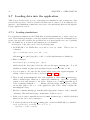
Loading data into the application . . . . . . . . .
2.7.1 Loading simulations . . . . . . . . . . . .
2.7.2 Adding the initial states to the definitions
2.7.3 Adding weight mapping to the definitions
2.7.4 Loading data into the repository . . . . . .
2.7.5 Description system . . . . . . . . . . . . .
.
.
.
.
.
.
.
.
.
.
.
3 Developer point of view
3.1 Architectural overview . . . . . . . . . . . . . . . .
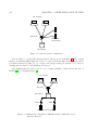
3.2 Top level component interconnections . . . . . . . .
3.3 Software packages used in the application . . . . . .
3.4 Python programming language . . . . . . . . . . . .
3.5 Brief introduction of YAML format . . . . . . . . .
3.6 YAML interface for MATLAB . . . . . . . . . . . .
3.7 Web browser part of the application . . . . . . . . .
3.7.1 jQuery . . . . . . . . . . . . . . . . . . . . .
3.7.2 Bootstrap . . . . . . . . . . . . . . . . . . .
3.7.3 Flot and graphs in the application in general
3.8 Web development – using a framework . . . . . . .
3.8.1 Django . . . . . . . . . . . . . . . . . . . . .
3.9 MATLAB . . . . . . . . . . . . . . . . . . . . . . .
3.9.1 How to call MATLAB from outside . . . . .
3.10 Data storage . . . . . . . . . . . . . . . . . . . . . .
3.11 What happens after clicking the Compute button .
3.12 Application components . . . . . . . . . . . . . . .
3.12.1 Data repository . . . . . . . . . . . . . . . .
3.12.2 Output series objects . . . . . . . . . . . . .
3.12.3 Task queue . . . . . . . . . . . . . . . . . .
3.12.4 Generic simulation . . . . . . . . . . . . . .
3.12.5 MPC simulation . . . . . . . . . . . . . . . .
3.12.6 MATLAB poller . . . . . . . . . . . . . . .
3.12.7 The MATLAB glue . . . . . . . . . . . . . .
3.12.8 Data transfer protocol for an assignment . .
.
.
.
.
.
.
.
.
.
.
.
.
.
.
.
.
.
.
.
.
.
.
.
.
.
.
.
.
.
.
.
.
.
.
.
.
.
.
.
.
.
.
.
.
.
.
.
.
.
.
.
.
.
.
.
.
.
.
.
.
.
.
.
.
.
.
.
.
.
.
.
.
.
.
.
.
.
.
.
.
.
.
.
.
.
.
.
.
.
.
.
.
.
.
.
.
.
.
.
.
.
.
.
.
.
.
.
.
.
.
.
.
.
.
.
.
.
.
.
.
.
.
.
.
.
.
.
.
.
.
.
.
.
.
.
.
.
.
.
.
.
.
.
.
.
.
.
.
.
.
.
.
.
.
.
.
.
.
.
.
.
.
.
.
.
.
.
.
.
.
.
.
.
.
.
.
.
.
.
.
.
.
.
.
.
.
.
.
.
.
.
.
.
.
.
.
.
.
.
.
.
.
.
.
.
.
.
.
.
.
.
.
.
.
.
.
.
.
.
.
.
.
.
.
.
.
.
.
.
.
.
.
.
.
.
.
.
.
.
.
.
.
.
.
.
.
.
.
.
.
.
.
.
.
.
.
.
.
.
.
.
.
.
.
.
.
.
.
.
.
.
.
.
.
.
.
.
.
.
.
.
.
.
.
.
.
.
.
.
.
.
.
.
.
.
.
.
.
.
.
.
.
.
.
.
.
.
.
.
.
.
.
.
.
.
.
.
.
.
.
.
.
.
.
.
.
.
.
.
.
.
.
.
.
.
.
.
.
.
.
.
.
.
.
.
.
.
.
.
.
.
.
.
.
.
.
.
.
.
.
.
.
.
.
.
.
.
.
.
.
.
.
.
.
.
.
.
.
.
.
.
.
.
.
.
.
.
.
.
.
.
.
.
.
.
.
.
.
.
.
.
.
.
.
.
.
.
27
28
31
32
35
38
38
40
40
41
41
.
.
.
.
.
.
.
.
.
.
.
.
.
.
.
.
.
.
.
.
.
.
.
.
.
43
43
43
45
45
46
47
48
49
50
50
50
53
53
54
54
55
56
56
57
57
59
60
61
61
62
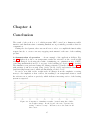
4 Conclusion
65
Bibliography
71
Content of the attached CD
I
Chapter 1
Introduction
Buildings as such consume approximately 40% of total energy. Nearly half of that is
put into HVAC (Heating, Ventilation and Air Conditioning), hence governments of many
states concerned about impacts of this fact on the environment issuing standards, regulating the consumption and promising further savings in this field for the future [36].
There are new houses built incessantly, which comply to these standards, but the
number of new buildings compared to the old ones is small and this ratio is changing
only slowly, thus engineers are looking for new ways to keep the trend of increasing the
savings by changing of structures which already exist.
It is possible to adjust or rebuild a part of the construction to achieve the goal,
but this is very costly. Another way of save up is to make the efficiency of energy
distribution in current buildings better, which can be done by engagement of Building
Automation Systems (BAS) or only by introducing new algorithms for existing ones
without an interference with physical aspects of a building. There were efforts of many
academic and industrial teams to implement various advanced control algorithms in the
area of HVAC [25, 31, 35, 30, 27].
1.1
Advanced control techniques for HVAC
There has been two main directions in the heating control research recently.
One group involves method of the artificial intelligence, specifically neural networks,
genetic algorithms, fuzzy methods and others.
The second group, which is in concern of this work, employs techniques based on
principles of the classical control theory, called Model Predictive Control (MPC). MPC is
in theory easy to formulate as it consists in direct application of optimization techniques
on the given control problem. It is widely used in many industry areas – see for instance
[33, 32, 34, 29] for further reading.
The idea behind MPC is to express a goal of the control by the terms of a cost function,
value of which can be called penalization. Minimization of the cost function results in a
control strategy, which also fulfils constraints given as a part of MPC problem formulation.
This optimization happens on the specific constant time interval, which is called prediction
1
2
CHAPTER 1. INTRODUCTION
horizon with the length specific for the control problem solved. Specifically for the HVAC,
the cost function is, roughly speaking, equivalent to energy consumed plus penalty for
some comfort requirement violation.
The key point, which really differs the technique from others is just mentioned MPC
factoring of given constraints into the control strategy, hence it predicts potential future
saturations and picks a control trajectory, which both minimizes the cost function and
does not violate the constraints all at once.
The technique heavily relies on availability of a controlled plant model, which makes
the process of plant model identification of a great importance.
To cover uncertainties and unpredictable disturbances of the controlled system, there
is a need of feedback to be integrated. So in the on-line implementations, the methodology
is applied as explained, but only the first point of the optimization result is used as an
input to the controlled system. Then in the next sampling period, the optimization is
performed again with the new measured data and the whole process is repeated.
1.2
Controlled plant
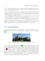
Specifically for this work, MPC is used for control of heating in CTU-FEE building in
Prague. Its description follows. Text and illustrations of this subsection are adopted from
[36].
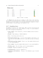
Figure 1.1: The building of Czech Technical University in Prague, Dejvice
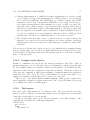
The building of the CTU uses Crittall [24] type ceiling radiant heating and cooling
system. In this system, the heating (or cooling) beams are embedded into the concrete
ceiling. A simplified scheme of the ceiling radiant heating system is illustrated in Figure 1.2. The source of heat is a vapor-liquid heat exchanger, which supplies the heating
water to the water container. A mixing occurs here, and the water is supplied to the
respective heating circuits. An accurate temperature control of the heating water for
respective circuits is achieved by a three-port valve with a servo drive. The heating water
is then supplied to the respective ceiling beams. There is one measurement point in a
reference room for every circuit. The set-point of the control valve is therefore the control
variable for the ceiling radiant heating system in each circuit.
1.2. CONTROLLED PLANT
outside
temperature
3
temperature of the input
water to the ceiling pipes
ceiling
radiant
heating
reference
room
temperature of the
ouput water from
container
inside temperature
heat
exchanger
temperature of the
output water from the
ceiling pipes
container
Figure 1.2: Simplified scheme of the ceiling radiant heating system
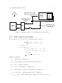
1.2.1
MPC problem formulation
Direct formulation of the problem of building heating control is:
min
u
N
−1
X
(|Rk uk |s + |Qk (yk − zk )|t )
k=0
subject to:
Fk xk + Gk uk ≤ hk
xk+1 = Axk + Buk + V vk k = 1 . . . Ny
yk = Cxk + Duk + W vk k = 1 . . . Ny
x0 = xinit
rk ≤ zk ≤ rk k = 1 . . . Ny
With these quantities:
• xk – system state of dimension nx
• uk – system input (controlled variables) of dimension nk
• yk – vector of system outputs ny
• vk – vector of disturbances of dimension nv
• zk – slack variable on the zone temperature of dimension nz
• s, t – norm order of particular parts of the cost function
• x0 , xinit – state at time 0, initial state, dimension is the same as for xk
4
CHAPTER 1. INTRODUCTION
• rk , rk – minimal and maximal reference variable for the system outputs, dimension
is the same as for zk
• N – prediction horizon, positive integer number
• k – discrete time, integer number, k ∈ 0 . . . N − 1
• A, B, C, D – system matrices of appropriate dimensions
• V, W – matrices of disturbance input of appropriate dimensions
• Qk , Rk – weighting matrices of appropriate dimensions which express trade-off between reference tracking and energy consumption
• Fk , Gk , hk – matrices/vector, of appropriate dimensions, defining constrains of system states and input variables
This is application of the technique just mentioned. Weighted energy equivalent is penalized in s-norm, while weighted reference band violation is penalized in t-norm. First
sharp inequality reflects the physical limits of the system. Second inequality constraints
the slack variable of reference band.
The slack variable is artificially introduced variable, which serves for penalizing given
variable, which is attached to, only when it escapes given interval (system output in our
case).
1.3
Current controller implementation
At the moment the development of the application started, there was an MPC runtime
(HVAC control system) established. The controller in this runtime is implemented in
MATLAB and takes into account:
• Disturbance predictions – This is a weather forecast, which includes mainly an
ambient temperature and also partly a solar radiation power.
• Considers future references – Controller has a knowledge of future requirements of
a temperature, which allows it to prepare controller plant for the reference change
before it starts.
• Keeps constraints of a plant – Takes into account maximal ratings of all controlled
variables (minimal and maximal water temperatures, maximal speed of temperature
change).
The system reads input data first. Data is used to formulate the optimization problem,
for which YALMIP toolbox [21] is employed. Then a solver is called to obtain the solution.
There is mainly sdpt3 solver [15] used, also SeDuMi solver [16] was engaged, but evinced
worse results mainly with longer prediction horizons. Computed results are eventually
written to disk.
1.3. CURRENT CONTROLLER IMPLEMENTATION
5
The MPC runtime stores the data and even communicates with PLC using YAML
(more in Section 3.5) files, stored locally on the disk of the machine, which performs
on-line computations. One of the key points of the application being developed is to
emulate this communication and use the system as just described for off-line simulations
with only small changes.
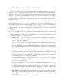
YAML files have special structure, convenient for the purpose of the controlling problem. To read the files, there is YAMLMatlab (see Section 3.6) interface used, which
implements a kind of inheritance and allows to merge several files into one data structure. Files are organized beginning with the most general level, where for instance the
variable classes are defined with their default items (for example maximal temperature).
The fields of these classes are then successively specified by another files as needed. For
example when there is some element of the class with the maximal water temperature
set and this value is different from the one defined in the class which the element comes
under, the value is overwritten by the one of the more specific class.
After YAMLMatlab merges the files, the structure is as follows (only important fields
stated):
• variables – Defines all possible variables which may occur with their default values,
constraints, units etc.
• data – Actual data, processed by the controller. Important part of the on-line
implementation, but not used in the application, because of inefficiency.
• controllers – Contains key-value map, which holds settings of all controllers,
defined in the system. Each value of this map is another map, containing these
key-value pairs:
– predictionHorizon – Prediction horizon length in seconds.
– solver – Specifies which solver is used for computation and its settings.
– costFunction – Key-value map, each item stands for a part, added to the
cost function. Adjusts the soft constraints.
∗ norm – Determines the norm of this cost function part.
∗ weight – Holds the value of weight of this part.
∗ refMin/refMax – When set, it sets constant minimal/maximal constraint
of the variable, weighted in the cost function. The band between values is
not penalized, locations outside are weighted by the value of weight field.
∗ refMinSchedule/refMaxSchedule – Same as preceding, but with a variable constraint. The value is a reference into data part of the structure,
where the constraint is stored.
– constraints – Hard constraints.
∗ refMin/refMax – When set, introduces a constraint on the specified variable, which must not be violated by a solver.
∗ refMinSchedule/refMaxSchedule – Same as preceding, but instead of
constant, uses variable as a constraint. The value is a reference into data
part of the structure, where the constraint is stored.
6
CHAPTER 1. INTRODUCTION
• models – Key-value structure, each item of it holds the information about one
model in the system.
• controlSamplingPeriod – Sampling period of the model discretization, in seconds.
• defaultInitialState – Vector of the state, which the model is initialized to.
In the current HVAC, there is also a script called ’MPC Viewer’, which reads the
results, and plots them on a web page, which serves as a diagnostic tool for the online
process.
Another group of YAML files is used to store the information about which data is
plotted and about grouping of these data into charts. The structure of these files is:
• Root of the file is a dictionary with only one key, named PlotDefinition. The
value under this key is a list, which contains a number of dictionaries. Structure of
each that dictionary is:
– Title – Determines the title of the chart.
– Variables – Groups variables, which should be displayed all in one figure. It
is a list of dictionaries, each of them with following items:
∗ ID – Identifies, which variable, specified in YAML definition files, will be
plotted.
∗ Color – Color to plot the series, expressed as a hexadecimal RRGGBB triplet.
∗ Description – Name of the series to be displayed in the legend.
1.3.1
The off-line simulation of the system
Running the system without the connection to the underlying PLC is used to tune the
controller, to explore energy savings and to study possible failure of the controller.
The simulations run are short-term, covering the length of the prediction horizon. This
strategy of studying the MPC is based on the idea that when the system behaves well on
one prediction horizon (typically three or four days long) in all characteristic situations
(heating up after a weekend, day-night transitions etc.), this induces that it will be likely
to behave well also in closed loop. This is in contrast in long-term approaches (BACTool
[3], for example), which evaluate a mean behaviour of the controlled system over a long
time in order of months or a year.
1.4
Motivation of the application
When the engineer wants to run a simulation of a control problem, he or she has many
possibilities, how to do that. The system plentifully mentioned throughout this work,
MATLAB, is only one example.
1.5. BASIC REQUIREMENTS FOR THE APPLICATION
7
The problems of these systems are often their complexity, paradoxically their featurerichness, need to learn special kind of de-facto programming language, which cause the
novice to be easily lost within.
Mentioned systems are often hard to maintain even for a lecturer during a speech,
presenting some control problem and their appearance can be confusing for a speech
participants, who can only watch what the lecturer does in addition.
There are some applets and simple tools easily found on the internet, dealing with
control engineering branch, even with MPC, but they are all actually textbook examples,
with no background in some real specific system, much less with the ability for user to
define his/her own control problem in some non-trivial way.
Another aspect is that specifically MPC simulations are known to be time consuming
even on some better hardware. Some tool could offer to perform a long-lasting simulation
from some very low-end netbook, but with the actual computation distributed to some
really powerful hardware, shared with other users of the application. This system could
moreover allow the user to run more simulations at the same time, which, distributed on
several computation cores, are finished faster than in the case they are run on a standard
desktop all at once.
1.5
Basic requirements for the application
The system will be operated using a web browser and, generally speaking, it will allow
to launch simulations on some remote computational core (currently MATLAB).
Specifically it will simulate one optimization step of a predictive controller on a defined
model-controller (building-MPC) pair from the set, loaded into the system. Subsequently
it will give an ability to clearly display the simulation results and especially to explore
changes in a behaviour of the controller in the dependency on its settings in an illustrative
way.
The work with the software can be divided into two base levels:
Manager level, which will make ordinary people to become familiar with the practice
in heating systems design with the MPC method by use of a simple interactive interface,
which will in fact allow them only:
• to display a prepared assignment template.
• to change one or at most a few simple parameters of a simulation (for example one
number, which for given simulation determines a trade-off between heating comfort
and heating cost).
• to launch the simulation.
• to display resulting data series in relation with the system inputs and compare more
results with each other.
• to be able to return to the assignment, change some parameter and launch the
simulation again.
8
CHAPTER 1. INTRODUCTION
Engineer level, which will serve to validate mathematical model of the building.
The user with an expert knowledge of the building will be able to show that the heating
system behaves correctly or poorly with the given conditions. This interface will be more
complex, with the functionality approximately same as the previous one, but in addition:
• There will be a possibility to combine various input data series with more freedom
and control over the settings.
• It will be possible to fine-tune the simulation settings, especially the weights of
particular variable penalization for the MPC strategy.
All results should be some way archived in the user’s workspace for further return to
the simulations already finished, in the future.
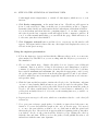
1.5.1
Structure of solved problem
For the purpose of the application design and its clearance, there was a data structure
sketched which captures the entities, important for the application. The structure as
mapped to the application has following parts:
Prediction horizon This is a constant floating point value in the units of hours, predefined to be between 8 and 168.
Initial conditions Setting, expressed by combobox filled with initial condition sets,
defined by administrator. There is also one item crossed out, which means that no initial
state will be provided to the simulation and it is in its responsibility to use some default.
The initial condition will be mostly an equilibrium or another interesting state.
Constraints This block contains hard constraint settings of the controller. It is a list
of variables for which you set the constraint. Each item of this list has minimal and
maximal value, which can be each fixed or variable. 1
Cost function This block is a bunch of cost function contributor variables. For each
there can be set:
• Norm – 1-norm, quadratic norm and infinity norm
• Weight – floating point number higher than zero.
2
• Minimal and maximal value – each can be either fixed or variable as in the
Constraints block.
1
At the time of writing this document, variable hard constraints are not yet implemented in underlying
MPC scripts
2
In current implementation of underlying MPC scripts, there is an effort to normalize weights, so
values between 0 and 1 should make the best sense.
1.5. BASIC REQUIREMENTS FOR THE APPLICATION
9
Disturbances List of input disturbance variables. Each has variable content – the data
series cut-out.
Overall weight This is simply a set of ’One big cost settings’ for the whole control
problem. When the simulation has the Manager interface set, it is remapped to the
weights in Cost function block, which are overwritten by these new values.
User description This is place where you should briefly and clearly describe specifics
of your current simulation setting to distinguish between more simulations created from
the same template.
10
CHAPTER 1. INTRODUCTION
Chapter 2
User manual
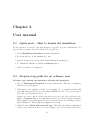
2.1
Quick start – How to launch the simulation
For the system to be usable, some user should be logged in. Log in by clicking the User
menu in the top right corner. It is labeled ’Not logged in’.
1. Select Simulations/Templates from the main menu.
2. From the list, choose the simulation to run.
3. In the following form, it is possible adjust simulation parameters.
4. To launch the simulation, click the Compute button.
5. Wait for results to be displayed.
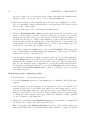
2.2
Step-by-step guide for an ordinary user
Creating copy, running the simulation, aborting the simulation
1. Choose Simulations/Templates from the main menu. The list of templates,
visible by you, will appear.
2. Click name of the template you like. For beginning, choose template marked with
green M, which will lead you to the simpler simulation form. Now you can explore
the form, read descriptions and so on.
If there are some controls on the form, they are greyed out. Moreover there is no
Save or Compute button. It is like this because you are just viewing a template.
This template is probably shared by more users and serves as a starting point for
their simulations. This is why the template is read-only.
3. Click the button Work with unsolved copy. This will copy whichever simulation
form you see and sets it up to be your working copy. You are then redirected to
11
12
CHAPTER 2. USER MANUAL
the form of that copy. You will notice that a button bar under the simulation title
changed because you are now able to do more with the simulation.
4. Fill in the description. Use something short and clear, say, ’emphasized economy’.
Choose some initial condition and use slider to set desired trade-off between comfort
and economy – slide it right.
5. Now you want only to save your changes, use Save button.
6. Navigate Simulations/My copies from the main menu and you will see your
newly created working copy there, described with text you entered. You can also
navigate the Template listing page again and you will notice that the number on
the button in the Copies column of the template you just copied increased by one.
Click the button with the number and you should again see your working copy
in the listing. Now use browser Back button or click on the working copy User
description to get back to the working copy form.
7. You want to launch the simulation process now; click Compute. This button will
save potential changes and then enqueue the simulation for processing. You will be
redirected to the Live computation log.
8. You can wait for simulation to finish or continue your work. To abort the simulation,
click the Abort button. You will be redirected back to the simulation form, but the
simulation will be marked as Aborted and will be read-only. This is because there
may be some messages in the computation log and some results already present.
To check the partial result and the log, you can click Result button in the button
bar. But now click Clear solution and you have your working copy as you would
never have started it.
Displaying results, comparing results
1. Repeat steps 1. . . 4 from the previous list.
2. Now click Compute and wait for the simulation to be finished. The Results page
appears.
3. Pan the figures by mouse dragging, use mousewheel to test zoom. Switch zoom
restriction buttons above the figure and explore how this changed the zoom behaviour, click magnifier buttons to perform wheel-less zoom. Finally click button
with the crossed circle to reset the view. Drag the figure (in the area near its title)
to change the order of figures on the page. This can be useful if you like to quickly
see two far figures on the same place.
4. Change series visibility using Displayed series dropdown menu. You must click
the checkboxes to achieve the effect, not their label.
5. Hide some figures using Displayed figures dropdown, located in the button bar
under the ’Results’ title. For example imagine that you like to compare North and
2.2. STEP-BY-STEP GUIDE FOR AN ORDINARY USER
13
South supply water temperatures, so switch off other figures, which are not of your
interest.
6. Click Series comparator on the main button bar. Checkboxes will appear in
front of each series label. Turn on checkboxes of series which you like to compare.
Remember that checkboxes will remain checked when figure with them is hidden –
if you check them and then hide the containing figure to do another comparison,
the series from the last comparison will still appear in the comparator window. If
you do not like manual unchecking, you can refresh the page, which will restore it
to the state just after it has finished.
7. Click Compare selected button and the Series comparator modal window will
appear. The figure inside behaves like any other figure and displays the series you
selected in the previous step.
Using the engineer presentation
1. Follow the first step of previous list with the difference that you choose some template marked by blue M. Now you are working with the Engineer presentation of
the simulation.
2. Choose some initial state. Simple edit fields does not deserve some additional
comments. But it would be boring if all references and disturbances would be
constant. So change Room temperatures from the Cost function block to both have
have variable minimum and maximum (choosing this in appropriate comboboxes),
choose the appropriate data series from another just-appeared combobox for them –
it will be named in some clear manner (typically it will contain the word ’reference’
and specifier ’min’).
3. Click the button with bar graph to initiate the Graph picker. At this time only turn
on some coloured synchronization button, say, green one and close the picker. Time
points are synchronized by pushing the value selected at the moment the picker is
closed to all others, synchronized by the same coloured button combination. Not
pulling it from lastly selected. So if you choose the starting time now, you will loose
your selection.
4. Repeat previous step for all series, which are somewhat related to each other (all
references).
5. Now open some reference graph picker, for which you just selected the sync combination. You can deal with the graph as the ones on Results page. If you need
to, zoom to the part which you want to choose, click button with the pencil and
then in the plot area. Green selection appears with its beginning in the point where
you clicked. Or choose the point from the Calendar picker clicking the edit box
with the date and time. When you close the picker, it will publish its value to all
subscribers with the same sync signature.
14
CHAPTER 2. USER MANUAL
6. Time point selections are persisted including the state of synchronization buttons,
so do not worry, if you need to do this ’clicking procedure’, you probably will have
to do it only once. Persist the form using the Save button.
7. Do the same steps for disturbances if there are more than one.
8. Launching the simulation is exactly the same process as described above.
Running multiple simulations, checking the queue
If you need to compare more simulation results, you will probably feel the advantage of
having more workers able to deal with your tasks.
1. Start some simulation. The knowledge of how to do it can be found in previous
lists.
2. When you are in Live computation log do not wait for the simulation to finish. Set
up another simulation using the main menu. Better said: Repeat from the first
step until you have enqueued all simulations you wanted.
3. You probably noticed white ’play’ arrow, which appeared on the right side of the
Simulations menu. Whenever the arrow is there, it means that you have some
tasks in the queue or some tasks just being computed on workers or both. When
all your tasks are done, the arrow disappears. This will happen when you navigate
to another page or automatically – the arrow state reloads itself every 30s.
4. If you have feeling that the computation takes too long, you can go for Processing/Task queue to see where in the queue you are. You can look for your user
name in Owner column or just look for content of Task column, which has a blue
colour. This means that the task is accessible by you hence it is probably your task
(unless you are an administrator – in that case, all tasks are yours in principle).
5. When all your tasks are finished, you can display their results all at once to be able
to compare them. Go to Simulations/My results. Sort the list clicking the Last
touched column twice in order to sort it descending by the time when tasks were
finished.
6. Choose tasks for result comparison turning on appropriate checkboxes on the left.
7. Click Show results at once, which will navigate you to the Results page, where
you can see results of all simulations selected. Now use techniques you learnt in
previous listings.
To revise: Hide resulting figures of all simulations you are not interested to. After
this step you will probably end up with simulation result block with one figure per
one simulation. Turn on the comparator and select series to compare. Then launch
the comparator dialog.
2.3. STEP-BY-STEP GUIDE FOR AN ADMINISTRATOR
2.3
15
Step-by-step guide for an administrator
Adding users and groups
The concept of users and groups in Django and so in the application is probably the same
you are used to. Groups are utilized basically to associate more templates to more users
in some comfortable way.
1. Select username/Django admin from the main menu, where username is the
name of the user currently logged in and there must be the sign (SU) after that
name, which indicates that the user is a superuser, otherwise the Django admin
choice will not be displayed. In the admin interface, choose Groups.
2. Create one group using Add user at the top right corner of the window.
3. Go to admin home (link at the top left corner of the window) and click Users.
4. Now you see the listing of all users registered in the system including additional
information about them. Add several users using Add user at the top right corner
of the window. Users you now added are ordinary users.
5. In the listing, click on each username of newly created users and in Groups block
select the group you just created. Then click Save. If you like to make the users
being administrators, check Staff status and Superuser status for them. But do not
activate this now, we need just ordinary users for the next instruction list.
Publishing templates to users
1. In Django administration, click Generic problems, then click on the simulation
you want to associate. The page you just navigated to can be also navigated from
the simulation form using Administer this simulation or from the listing of
simulations clicking the button with the icon of gear.
2. In the administration page of simulation, choose group you created in steps of
previous list in the Viewer users block. Additionally you can afterwards create
yet another users and associate them some simulations individually in the Viewer
groups block. At the end of each modification click Save.
3. Log out and then log in as some user you created. Check that he or she can see
simulations you associated him or her and that he or she can operate with them.
Remember that if you have turned on the is public flag of some simulation, this
simulation will appear in the listing of templates of every user (if it is a template)
even if you have not explicitly associated it. In addition if you set is public flag for
working copy (solved), it will appear in the listing of working copies (plus in the
listing results) of the associated user. The user then will not be able to delete it
because he or she will not be owner of this simulation (unless you set the user to
be the owner), which might be confusing for him or her.
16
CHAPTER 2. USER MANUAL
4. If you want to cancel all associations to users or groups of more templates, you can
do that as a bulk operation. In the Django admin, go to the Generic problem listing,
turn on checkboxes belonging to the simulations you like to cancel associations for
and then use appropriate action from the combobox labeled Actions, located above
the listing and click OK.
Setting up a template
When simulations are inserted to the system, they are set to some default state. The
script, assimilating the simulations, will make an effort to set up the simulation for
you, using supplied YAML files by setting weights, norms, prediction horizon, constant
maxima/minima and so, but will not be able to infer some details, for example which
disturbance and from which time you like to choose.
The approach to fine-tune the simulation follows.
1. Choose some template you want to set up. Go to its administration. You learnt
the knowledge of how to do so in previous instruction listings. You do not need to
choose a template, every simulation can be turned into a template and back, which
ability we will now utilize.
2. On the administration page, uncheck Is template flag and set Presentation to
Engineer, which will consequently allows you to edit largest possible set of parameters. The parameters will be still there if the choosen presentation will be
finally Manager. The key is that Manager presentation will hide the parameters,
but use them all as a resulting problem set-up unless something (some weights) gets
overriden by overall weights.
Just for case, remove all associations the simulation may have to users and groups.
Click Save and continue editing at the bottom of the page, then View on site,
which will lead you to the simulation form of the problem.
3. Set simulation parameters as you like, run several iterations of its computation to
check whether you set it correctly. Then clear the simulation results. Remember
to Save or Compute the simulation to persist changes you made.
4. Optionally – if you plan to make the simulation presentation to be Manager – go to
the administration page of the simulation and select Manager presentation. Then
again View on site. Now choose the default state of Overall weight sliders, then
– again – do not forget to persist the changes.
5. Finally go to the simulation administration again and check Is template there.
Additionally you can associate it some descriptor.
You now have your brand new template. Associate it to some users, log in using
their accounts and see whether it works as expected.
2.4. THE APPLICATION IN GENERAL – ORDINARY USER POINT OF VIEW 17
2.4
2.4.1
The application in general – Ordinary user
point of view
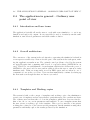
Introduction and base terms
The application basically allows the users to work with some simulation – to set it up,
launch it and explore its output. It can especially be used to iteratively run the same
simulation, tune selected parameters and track results evolution.
2.4.2
Overall architecture
The cornerstone of the system is the web interface, expressing the simulation backend in
a non-expert accessible way. Next noticeable part of the system is the task queue, making the application asynchronous. The optimal control problems, solved by the system
are typically quite time consuming with a need of a special software (MATLAB in our
case). This led to an establishment of a mechanism, which in fact delivers the power of
MATLAB to the user’s web browser and in addition allows the user to run more tasks
simultaneously. Tasks are temporarily stored in FIFO queue and are taken by one of
computation cores as the core is free. User can then immediately continue by setting up
the next task even though the first one has not yet ended.
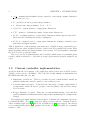
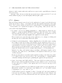
2.4.3
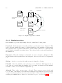
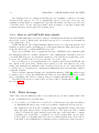
Templates and Working copies
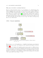
The system is built on the concept of templates and working copies. An administrator
creates a set of templates and associates them to particular users, who can then use them.
The ordinary user can then take a look at the templates, which have been associated to
him or her, choose one, set its parameters and launch it. To use a template means that
the user creates a working copy of the template. This copy becomes his or her private
working place, where he or she can set various parameters, run the simulation using these
parameters and finally explore the results produced by the simulation.
18
CHAPTER 2. USER MANUAL
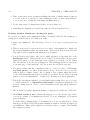
Results
Explore results
Templates
Choose template
to work with
Selected
template
Working
copy
Create copy to be
private for user
Working
copy
Launch computation
Figure 2.1: Simplified application workflow
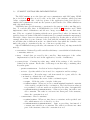
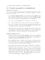
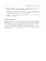
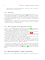
2.4.4
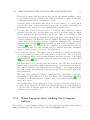
Simulation states
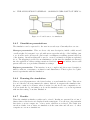
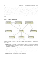
Each simulation goes through a simple lifecycle, which has following states:
Unsolved At the time user creates the working copy, the state is set to Unsolved. This
is the only state, which allows user to edit the parameters of the simulation. Other states
may signal presence of partial results and log items, which would not be consistent with
saved changes in simulation settings, hence other states disable saving and launching of
the simulation.
Enqueued When the simulation is launched, its state is changed to Enqueued. This
means that the task was pushed into the task queue, but not yet received by computation
core.
Solving As the core receives the task, its state is changed to Solving.
Finished After the simulation run, the state is set to Finished. This happens also in
case of an error, raised during the simulation. You can find out whether the task finished
normally or due to an error in the computation log.
Aborted There is also one more state – Aborted. There are more reasons for the task
to be aborted – the task is aborted when it is enqueued longer than its enqueued timeout
or is processed longer than its processing timeout, but as for user, the most obvious reason
is hitting the Abort button on the live simulation log page – see Section 2.6.11.
2.4. THE APPLICATION IN GENERAL – ORDINARY USER POINT OF VIEW 19
Figure 2.2: Possible states of a simulation
2.4.5
Simulation presentations
The simulation can be expressed to the user in several ways. Currently there are two:
Manager presentation This one shows only user description, initial conditions and
overall weights. It is meant for people without an expert knowledge of the building, just
to see how the trade-off between comfort and cost influences resulting system behaviour
of the heating. Overall weights will be used to create Cost function weights as explained
above. The mapping is created by an administrator at the time the simulation is inserted
into the application. Other settings, mentioned in Section 1.3.1 are hidden, but are still
present and serve as a predefined simulation settings.
Engineer presentation This interface is more complex and shows user description,
initial conditions, constraints, cost function and disturbances. This is a place for sophisticated experiments with the simulation.
2.4.6
Running the simulation
When you set all parameters to the desired values, you can launch the solver. This action
does not directly call some numerical routines. Instead, it enqueues the simulation into
the queue, common for all users, where it waits for some free-for-use computation core.
You can watch the log, informing you about the simulation state or you can experiment
with another setting or another simulation.
2.4.7
Results
When the simulation finishes, results can be viewed. Results are presented in a form of
charts, where related series are displayed in the same figure. You can view only particular
data series, you can compare two or more series, which are not related. The result view
can show results of more than one simulation at the same time and allows to do these
comparisons over more simulations.
20
CHAPTER 2. USER MANUAL
2.4.8
Simulation visibility
There can be simulations of more distinct systems or of a different kind in the application.
For the user not to be lost, while seeing all simulations in the system, there are some
relations between users and simulations possible. Moreover it is a good habit to found
some security rules, even simple, to increase user comfort (specifically others will not
silently change your simulation parameters and clear results and so on).
When you log in, you see only simulations, which were assigned to you by an administrator plus you see results and working copies, you have made.
After login you can typically see the list of templates, of which you have a read
privilege, because an administrator created a viewer relation between you or your user
group and these templates.
As you create a working copy, you are becoming an owner of the copy, which gives
you write access and allows you to enqueue it for computation.
2.5
2.5.1
The application in general – Administrator
point of view
Simulation visibility
One of the most noticeable differences that you are behaving as an owner to all simulations present in the system. That means you can view, edit, launch and abort foreign
simulations.
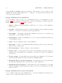
2.5.2
Administrator interface
The next big difference is that an administrator has access to the admin area, where some
additional settings of the system can be changed:
• Add, delete and change users and join them to groups.
• Add, delete and change user groups.
• Change some properties of simulations:
– Rename and delete.
– Assign template to users or groups.
– Change user description.
– Create, delete and assign simulation descriptor (simulation parameter legends,
general introduction).
– Change public flag of the simulation (turning it on make the simulation visible
for all users, even anonymous).
2.6. WALK THROUGH THE APPLICATION
21
– Change template flag of the simulation (turned on makes the simulation behave
like a template).
– Change simulation presentation (Manager, Engineer).
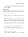
2.6
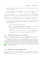
2.6.1
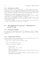
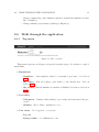
Walk through the application
Top menu
Figure 2.3: The top menu
This menu is present on all pages except the description page. It contains a couple of
useful links:
• Simulations
– Templates – List templates visible for currently logged user. See Section
2.6.2.
– My copies – List all working copies visible to the current user. More in
Section 2.6.3.
– My results – List all simulations, marked as Finished. Read more in Section
2.6.4.
• Processing
– Task queue – Display tasks waiting for processing and tasks just being processed.
– Workers – Show online computation cores.
• User menu – ’Not logged in’ or username
– Log out
– Django admin – for administrator only
22
CHAPTER 2. USER MANUAL
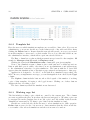
Figure 2.4: Templates listing
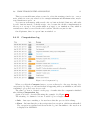
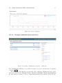
2.6.2
Template list
Here the user sees which simulation templates are accessible to him or her. If you are an
administrator, you can use checkboxes on the leftmost side of the table and delete them
clicking the Delete button. Beware that this removal will cascade on every copy created
from this template so users can loose their results. If you do not like this behaviour, use
the administrator interface, which will not perform cascaded deletion.
The Pre. column lets you know which presentation type is used for the template. M
stands for Manager view, E stands for Engineer view.
Clicking the item in the Simulation name column will open given template.
Next to the Simulation name column is place with buttons for additional actions:
Button with little gear is visible only when you are an administrator and will navigate
to the administrator interface for given simulation. The button with the ’i’ letter will
appear when the simulation has a description page assigned and navigates to that page.
Application is designed to be able to work with more simulation types than only
MPC. In case you implement a new type, you can distinguish it from others by the Type
column.
The Copies column includes buttons, whose label equals of the number of working
copies of that template, belonging to the logged in user. Clicking one of these buttons
displays the list of working copies.
The last column says when the simulation was last saved.
2.6.3
Working copy list
The list includes working copies, which are owned by the current user. The columns
are same regardless the place from where the list was navigated to (Working copies can
be navigated from the template list, from ’My copies’ and ’My results’ items from the
’Simulations’ menu and by ’Working copies’ button in the simulation form).
Checkboxes on the left side allows the user to select simulations for bulk operation.
Delete button serves for the obvious reason. Just remember that the deletion will also
cover results of the selected simulations and the action cannot be undone.
2.6. WALK THROUGH THE APPLICATION
23
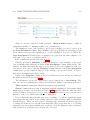
Figure 2.5: Working copies listing
There is one more button for bulk operation – Show results at once – which is
particularly useful for comparing results of more simulations.
The simulation form of the working copy is viewed clicking on a label or an icon in
the User description column. Every simulation has associated the user description text
block, which serves as a ’fine identification’ of every simulation. If you do not fill in the
User description field and create for example ten copies from the same template, you
will easily loose control over which is which.
Pre. column was described in section 2.6.2.
Clicking an item in Template column will navigate to the template of the given
copy. Remember this difference from the User description column, which leads to the
actual copy. Especially when the user does not annotate his or her simulation with user
descriptions, it is easy to click the Template column instead of the User description
column and copy the template instead of the existing copy by an accident. So try to
annotate your simulations when possible.
Right of the Template column is place for additional operation buttons, which are
the same as described in section 2.6.2
The information about who created the copy is found in the column Owner. The
user, who is not an administrator will probably find here himself or herself in most cases.
Time created column says when the particular copy was made.
Status column indicates what is happening with the simulation. Used terms, which
might appear in there are described in section 2.4.4 with the difference that the state
Solving is named Processing on worker name instead with worker name being the identification of the core, which deals with the computation.
It is worth mentioning that this page is not ’realtime’, e.g. when you find the status
here saying that the task is in processing, this label will not change until you manually
refresh the page. There are more pages containing some information which is expected
to change anon but are not refreshed automatically. These pages have the footer saying
when the page was generated which was an effort to hold the displayed data consistency
without the need of having each odd page auto-reloaded.
24
2.6.4
CHAPTER 2. USER MANUAL
Result list
This page looks the same as the one showing working copies of the user, but the content
is filtered to show only Finished and Aborted simulations.
2.6.5
Task queue
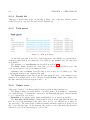
Figure 2.6: Task queue listing
As the title says, this is the view of the task queue. Specifically you can find here:
enqueued tasks, task in processing and done tasks for five minutes since the time they
were finished.
The meaning of column Status was described in section 2.6.3.
The Task column contains items of the form: user description (simulation name) and
each one navigates to the given simulation form.
Simulation has its Owner from the time it was created as a working copy. This
consequently indicates who enqueued the task.
The Last touch field informs about the time when the state of the simulation was
changed. For example when you see Enqueued in the Status column, this column gives
the time when the task was enqueued and so on.
2.6.6
Online cores
This is the overview of workers available in the system an their current jobs.
The Type column is actually matter of possible future. It is planned to implement
one additional type of ’equipment’ connected to the BuildingLAB queue, which is meant
to be a computation core starter.
Identifier is the unique string, which distinguishes one worker from another.
The Last sign of life before column is maybe relic from the past when the timeouts
have not yet been implemented and there was a need to see whether are workers are
’properly alive’. The value in this column determines when the application ’heard’ about
the core for the last time. At the moment, the worker record is automatically discarded
when it does not send any message for 30 seconds.
2.6. WALK THROUGH THE APPLICATION
25
Figure 2.7: Online cores listing
For Status maybe the name says everything. Possible values are Idle and Busy.
Here should be noted that when there is a task just being processed by the worker and
currently logged user has a right to view it, the Busy status will be displayed as a button
and will navigate to the just-being-processed simulation form.
2.6.7
Simulation form
All simulation forms have some common parts. There is an info about its state and
underneath is a button bar. Its content is different according to the current simulation
state. There can appear following buttons:
• Clear solution – Clear result and log of Finished simulation and set its state to
Working copy.
• Results – Open result page of finished simulation.
• Save – Persist changes made in the form.
• Work with unsolved copy – Copy the current simulation and navigate to its
form. If the the current simulation is solved, copy it without solution as a Working
copy.
• Work with copy from original – Create a copy of the template which was used
to create current simulation.
• Go to original – Open the template which was used to create current simulation.
• Working copies – Show all working copies from current simulation.
• Compute – Enqueue the simulation for processing.
• Computation log – Show live computation log.
• Administer this simulation – Navigate to the administrator page for current
simulation.
26
CHAPTER 2. USER MANUAL
Figure 2.8: The manager view
Underneath the bar you can find the text area to fill in your description. Fill in
something which describes what you changed in the form or what you are trying to show
using your simulation. Remember that first 128 characters of this field will appear in
User description column of table displaying working copies (Simulation listings and Task
queue) and you will use this description part to identify the simulation.
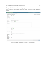
2.6.8
Simulation form – the manager view
Picture of the view was placed in the previous section. As said earlier, the specific of
the manager view is its simplicity. So the only parameters the user can change here are
Initial condition and Overall weights.
The latter is set using the slider and graphical illustration of trade-off between comfort
and economical aspects of the problem.
2.6. WALK THROUGH THE APPLICATION
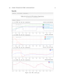
2.6.9
Simulation form – the engineer view
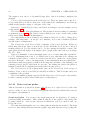
Figure 2.9: The engineer view
27
28
CHAPTER 2. USER MANUAL
The engineer view can be a bit mind-blowing place, but it is nothing complicated in
principle.
You see controls already known from Manager lab. There are many extra controls, so
it is possible that you will see help bars on the right if the administrator set them up,
which should explain content of each part of the form.
Best way to explain how does the form behave is perhaps to use the example as seen
on the picture 2.9.
The Simulation block is self-explanatory. The prediction horizon setting is constrained
as written in section 1.3.1. The Initial condition field is set to some concrete value, which
will be used during simulation initialization.
More interesting are the following blocks, which are tabbed to be able to change more
settings of the same kind – one tab per one constraint, one for each cost function addend
and the same for disturbances.
The Constraints block denotes hard constraints of the solved problem. Fields are
functioning almost the same as in next two blocks. Basically if you see the combobox
starting with word Use, the variable can be of both constant and variable content. The
appropriate field will change from simple edit to graph picker and back as you change
the Use... field.
There is a minimum of ’A2 north supply water’ set to be fixed with value specified to
be 15◦ C. Maximum value is set to be variable and you see that this choice changed an
edit field for fixed value to combobox for data series selection – in the case on the picture
the series ’Reference – max room temperature’ is used and finally there is graph picker –
small button with bar graph icon with text showing date and time of the starting point
currently selected (08/11/2011 14:06 in our case). By clicking the button the picker is
launched, which will be explained in detail in the following section.
The Cost function block is functionally same as the Constraints block except for
having a Norm combobox and Weight edit field in addition. This block introduces soft
constraints of the problem.
There are simulation inputs expressed in the Disturbances block can be only variable,
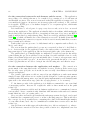
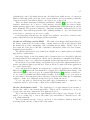
because constants would not have much sense for this purpose.
2.6.10
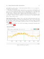
Data cut-out picker
This modal window as shown in picture 2.10, allows you to explore how does the data
series look like, zoom to see its details and pick the time interval, which will be used as
the input to the simulation.
Graph navigation You can move the graph using mouse by drag&drop. Zooming is
performed using mousewheel. Three leftmost buttons on the graph toolbar change the
zooming behaviour – they set the direction in which the view is zoomed in and out.
Follow the icons.
The buttons with magnifier are for zooming without using the mousewheel. The main
reason for introducing them was that the graph component used has a bug reading the
2.6. WALK THROUGH THE APPLICATION
29
mousewheel in some browsers, so when the mousewheel will not do as you expect it to
du, use these buttons instead.
The purpose of the button with crossed circle is to reset view to the default in case
you ’loose yourself’ during exploring. This can easily happen due to mousewheel bug
mentioned above, which by an accident sets the zooming parameters to such values that
the data cannot be displayed anymore using zooming and panning operations.
There always is a red data cursor, which allows the user to measure exact values found
in the figure. Measured values are updated on every mouse move and displayed in the
left top corner of the plot area.
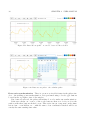
Time period selection Turning on the toggle button with pencil causes that every
mouse click in the graph area will move the starting time point to the location when
the user clicked. Time selection is represented by green area in the graph, its length
is automatically set to be the length of prediction horizon. For better explanation see
picture 2.11.
There is also possibility to choose the exact starting point using the datetime picker
as seen on picture 2.12.
Figure 2.10: Data cut-out picker
30
CHAPTER 2. USER MANUAL
Figure 2.11: Data cut-out picker – zoomed to better see the selection
Figure 2.12: Data cut-out picker – the calendar picker
Data series synchronization There is one more noticeable feature in the picker window – the starting point synchronization. It is performed using colored toggle buttons
located in the top right corner of the window.
If no button is selected, the picker will neither do nor be under any synchronization.
If the user checks one or more of the toggle buttons, then as soon as you close the
window with these buttons checked, every other series cut-out component on the simulation form – even hidden one – with the same colour combination checked will be set
exactly the same starting time value.
2.6. WALK THROUGH THE APPLICATION
31
This is very useful feature when you need to select the starting point for two or more
series, which are some way related as for example minimum and maximum value, maybe
some disturbances and so on.
You can very well manage with exactly only one button checked. Buttons could easily
be radio buttons instead of checkbox-type ones, because the checkbox implementation
allows you to set up to 128 synchronization groups for one simulation form, which is
certainly more than you need in the whole system. Checkboxes just for fun.
On all pictures, there is a green button switched on.
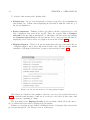
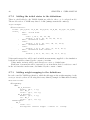
2.6.11
Computation log
Figure 2.13: Computation log
When you click the Compute button, you are redirected to the page showing Live
computation log. Here you can watch what is happening with your simulation, the table
containing log is polled every few seconds.
The same log view is obtained on the page of results after the computation finished
after clicking Computation log.
Again, it is best to describe this using the example. See Figure 2.13.
The meaning of columns is obvious. Possible log record types are:
• Info – Just says something to let user know that the process did not hung.
• Error – Informs that the worker script raised an exception, which was unhandled.
The exception is serialized and shown in the log, in form similar to the way how it
is displayed in MATLAB.
32
CHAPTER 2. USER MANUAL
• Debug – This will probably contain dump of some MATLAB variable or structure,
which will be displayed after clicking View record in the Message area.
• Wsnapshot – Signals that whole workspace has been just saved. The Message
area then contains the link, where .mat file can be downloaded and further be used
to track scripts action in case of an error or for an interest.
• Closure – This is mostly the last message of the log. It says how exactly the
computation was finished.
2.6.12
Results page
When the task is done it is possible to show its results. It happens automatically when
the user has the Live computation log displayed at the moment the simulation finishes,
which then causes the user to be automatically redirected to this page, otherwise the user
can open it from some page that contains working copies list by clicking an item in User
description column or clicking the Results button in the simulation form.
This page can show results of more than one simulation. In that case the results are
viewed one after the other – just imagine the page on the figure repeated several times
with different data.
2.6. WALK THROUGH THE APPLICATION
Figure 2.14: The result page
33
34
CHAPTER 2. USER MANUAL
To describe buttons under the ’Results’ title:
• Solution logs – Drops down a menu whose items correspond to shown simulations
and clicking one of them causes displaying modal window with the solution log of
the chosen simulation.
• Series comparator – Turning on this toggle button, checkbox appears before each
title of displayed data series in the legend. There also appears button Compare
selected beside the button just turned on. Checking some data series and clicking
the Compare selected button, the user fire the Series comparator modal window,
displaying selected series all in one graph as shown in the Picture 2.16.
• Displayed figures – This is a dropdown menu where the user can restrict the set
of displayed figures only to those important for him or her. The dropdown contains
identifiers of all figures divided into groups as shown in the Picture 2.15.
Figure 2.15: Dropdown menu for selecting displayed figures
The behaviour of figures is very similar to the Data cut-out picker described in section
2.6.10 – with the same meaning of buttons above the plot area, the red data cursor and
the same system of panning/zooming.
The new thing is the Displayed series dropdown menu, which allows the user to
choose which data series will be displayed in given figure.
If there is a description page defined, clicking the name of arbitrary data series in the
plot legend navigates to the Outputs section of that page.
2.6. WALK THROUGH THE APPLICATION
35
Figure 2.16: Series comparator
2.6.13
Django administration interface
Figure 2.17: Django administration interface – main page
The administration interface is accessible from the User menu, the interface is captured
on picture 2.17.
The function of the interface is expectable and consistent. Clicking the label on the
main page (specifically Groups, Users, Generic problems, Object descriptions)
the user will get a listing of object of that kind present in the system. There are also
36
CHAPTER 2. USER MANUAL
actions Add and Change with clear meaning. The interface does not allow to add
simulations, because their structure is too complex to be expressed in the interface in
some well arranged manner.
Django administration of simulations
As one example for all you can look over administration page of one simulation, see the
picture 2.18. The meaning of all buttons is obvious, the meaning of editable items was
briefly explained in section 2.6.7. Just to specify:
• Owner – Changes the user which is considered to be a creator of the simulation
being edited.
• Is public – When checked, the choice causes the simulation along with its potential
solution to be visible for anonymous (not-logged-in) users.
• Is template – Determines whether the simulation is treated as a working copy
(unchecked) or as a template (checked).
• Presentation – Allows an administrator to choose between available presentations
of the simulation form.
• Name - Allows editing the name of the simulation.
• Descriptor – Combobox determining which description will be used for given simulation. More on this below.
• User description – Allows a change of user description.
• Viewer users – Selects which users will see this simulation in their Templates
listing (in case the simulation is a template) or in My copies/My results listing in
case it is not.
• Viewer groups – Selects which user group will see the simulation. For all users
in given groups applies the same as written for Viewer users.
• Maximum time to wait for dequeuing – Sets the time in seconds, after which
the enqueued simulation will be aborted if no worker dequeues it.
• Maximum time for solution – Sets the time in seconds, in which the core dealing
with the simulation must manage its solution. If it does not manage it, the task
will be aborted.
Django administration of object descriptions
To be complete, this allows the administrator to relate the simulations with given descriptor. More on this in separate section below.
2.6. WALK THROUGH THE APPLICATION
37
Django administration of users and groups
These modules are present in the interface by default. Refer to the Django manual for
details.
Figure 2.18: Django administration interface – editing simulation
38
CHAPTER 2. USER MANUAL
2.7
Loading data into the application
This section describes the process of inserting new simulations and creating new data
series in the repository. Actions, described in this section, cannot be done using the web
interface. An administrator must have an access to the underlying database through the
Django application console.
2.7.1
Loading simulations
For creating new simulations, the YAML files, describing simulation for on-line control are
used. These instructions figure on the fact, that the system is cleaned from simulations as
next-to-last step will overwrite the specifications on workers but the new ones. Updating
the old definitions on workers is unfortunately not yet handled.
Assimilation of the data can be done in following steps:
1. In MATLAB, load YAML files, as would be done by on-line. This is done by
command:
spec = ReadYaml ( ’ main_file . yml ’ ,0 ,1);
with main file.yml being the root file of on-line implementation definitions.
2. Enter command
WriteYaml ( ’ spec_working . yml ’ , Spec )
which writes the data just loaded into the new file spec working.yml. Now all
simulation definitions (imported and mixed in) are written in this one file.
3. Now it is time to decorate the file by the initial states and weight mappings. If
adding of these is needed, refer to Sections 2.7.2 and 2.7.3.
4. There is a file in buildinglab folder of the application, called admin routines.py,
which contains helper functions to insert new simulations. Open the operating
system console and navigate to the folder. In first rows of admin routines.py is
a line, beginning with pth = ’.... Ensure, that the string, which follows, contain
an absolute path to the root of the application (the folder, which contains the
buildinglab folder).
5. Execute command manage.py syncdb (with appropriate changes of the command
on Linux). This will start Django maintenance Python console.
6. In the console, issue command execfile(’admin routines.py’), which loads helper
functions into the console namespace.
7. Load the specification file spec working.yml, created in MATLAB by command:
with open ( r " spec_working . yml " , ’r ’) as f :
specdict = yaml . load ( f )
2.7. LOADING DATA INTO THE APPLICATION
39
8. For given model-controller pair, which is to be inserted, launch command:
gensim = specAssimilator ( specdict , ’ controller_name ’ , ’ model_name ’)
where controller name and model name, respectively, are names of the model and
controller in the specification files. gensim variable now holds the instance of Django
model GenericSimulation of the simulation just inserted.
9. Load appropriate definition of simulation outputs for plotting:
with open ( r " s o m e _ p l o t _ d e f i n i t i o n . yml " , ’r ’) as f :
plotdef = yaml . load ( f )
10. Enter command:
plotAssimilator ( plotdef , gensim . c o n c r e t e _ p r o b l e m _ o b j e c t )
which associates given plotting metadata with the simulation. Repeat actions from
step 8 to insert all model-controller pairs wanted.
11. After the insertion, execute:
specDictClean ( specdict )
which clears all specifics of the on-line run (data series, reference settings, etc.).
12. Save the cleaned structure by command:
with open ( r " c le an ed _f or _m at la b . yml " , ’w ’) as f :
yaml . dump ( specdict , f )
13. In MATLAB, load the file cleaned for matlab.yml using command:
spec = ReadYaml ( ’ main_file . yml ’ ,0 ,1 ,0 ,1)
Please consider switches on the end of the command (it is different from the one in
step 1). Especially the last one is important, because it disables the YAML importer
form performing inheritance. If the switch is not present or is 0, inheritance will
pollute your cleaned data by defaults from higher-level definition classes, which will
issue no error, but will probably lead to strange simulation results.
14. Save spec variable as file Spec01.mat:
save ( ’ Spec01 ’ , ’ spec ’)
15. Finally distribute the file Spec01.mat to the worker machines, into the folder
blab/scripts, located in the root of worker SW equipment.
40
2.7.2
CHAPTER 2. USER MANUAL
Adding the initial states to the definitions
There is a field added to the YAML definitions, added to the root of a selected model.
The model section of YAML may then look like (unimportant fields omitted):
dejviceTempA1 :
...
BLinitialStates :
fields : [ A1_S_Room , A1_S_RW , A1_N_Room , A1_N_RW , A1_S_SW , A1_N_SW ]
states :
name : ’ Cooled down ’
value :
state : [ 19.5 , 24 , 19 , 24]
initial : [ 19.5 , 24 , 19 , 24 , 26 , 25.7]
name : ’ Overheated south ’
value :
initial : [ 23.5 , 28 , 21.5 , 26 , 35 , 25.9]
name : ’ Overheated north ’
value :
initial : [ 20.5 , 26 , 22.5 , 30 , 27.8 , 36.1]
name : ’ Overheated both circuits ’
value :
initial : [ 23.5 , 28 , 23.0 , 26 , 37.2 , 38.7]
...
Values under state key will be used as initial measurements, supplied to the simulation
backend as variables, named by the content of fields.
Values under initial will be used directly as a vector of initial state.
Each item of states list will be expressed as one item list in Initial conditions control
in the web interface under name, determined by the content of name.
2.7.3
Adding weight mapping to the definitions
In each controller YAML specification, which should support the weight mapping for the
manager interface, there is following dictionary defined (example for MPCcontrollerB3):
MPCcontrollerB3 :
...
BLweightMap :
MAP1 :
B3_S_RoomCost :
dstVec : [[1.0 , 0.0]]
src : HW_1
srcVec : [[0.0 , 100.0]]
B3_S_HeatCost :
dstVec : [[0.0 , 1.0]]
src : HW_1
srcVec : [[0.0 , 100.0]]
BLhiWeights :
HW_1 :
value : 50.0
description : Overall weight - comfort vs . economy
...
2.7. LOADING DATA INTO THE APPLICATION
41
In BLhiWeights dictionary, there are Overall weights defined, which will express themselves each as one slider. Currently there is always only one. The value field determines
the initial value of the slider. Description is a string, which identifies the slider in the
web interface.
The value from the manager interface slider is transmitted into MATLAB. It is always
between 0 and 100. The value is transformed using linear interpolation with the XY grid
created by srcVec, dstVec respectively. src field is the identification of the source slider
from the BLhiWeights section. Resulting value will be used as a weight for variable with
the name being the same as a name of the key the transformation is defined in.
To make things clear: In the example above, there will be one slider created, which
will be labeled ’Overall weight – comfort vs. economy’ and will have a default value 50.
This slider will be identified as HW1 in MATLAB. After the simulation is started, slider
value 0 is transformed to 1 and stored as a weight of B3 S RoomCost. If the slider is
on value 100, the resulting value will be 0. Numbers inside this interval will be linearly
interpolated. Value of B3 S HeatCost is obtained by the same way, but the slope the
slope of the interpolating function is opposite to the slope of the for B3 S RoomCost.
2.7.4
Loading data into the repository
1. Run the Django maintenance console and load admin routines.py as described in
the previous instructions.
2. Some way load the data into the Python console workspace. There are many ways
how to do it, it depends on the format the data is stored in. Before loading to the
application database, the data must be formed to list of lists. Inner list must have
exactly two items, first of them is time in milliseconds (UNIX time * 1000), second
one is the value of the variable in that time. Example:
data = [[1.0 ,2.0] ,[2.0 ,3.0] ,[3.0 , -2.0]]
3. Load the data into the system:
modrep . RepositoryItem . new ( data , ’ Name to identify the series ’)
There is a routine, called saveSomeData in admin routines.py, which creates simple sinusoid. Study its code for a basic idea about how to create and store the data
series.
2.7.5
Description system
There can be a description associated to each simulation. The description is stored as a
plain HTML file in some static folder of the application web server, accessible from the
internet. The file self should make sense as a whole, because it can be displayed in the
when user clicks the button with the ’i’ letter.
The same file is used as a source of concrete descriptions for setting blocks in simulation forms. See the grey boxes on the Picture 2.9.
42
CHAPTER 2. USER MANUAL
There is a method load of jQuery library (more info in Section 3.7.1), allowing AJAX
load of a file, content of which is parsed as HTML and used as a content of given DOM
element. Nodes in the description HTML file are labelled using HTML class attributes,
corresponding to the names of the adjustments blocks being described. load function
is then used to locate the parts of the file into the appropriate places. There are many
AJAX requests initiated, but all but the first one will be replied from the web browser
cache.
The URL path to the file is stored in the ObjectDescription model along with
path to the resolver Java Script file, which will be loaded before any description. The file
provides the resolveHelp(helpClass, helpIdent) function, through which all requests
for description are passed through, making it the extension point of mapping between
described blocks and the description HTML file. To describe particular simulation, create
appropriate HTML file, the ObjectDescription object and associate it to the simulation
being described.
The resolver function is called for every described element with following attributes:
• helpClass – Cathegory of description. Can be one of following:
– ’constraints’ – Description of some tab of the Constraints block.
– ’costfunction’ – Description of some tab of the Cost function block.
– ’disturbances’ – Description of some tab of the Disturbances block.
– ’simulation-settings’ – Description of Simulation settings block for the
engineer interface.
– ’simulation-settings-manager’ – Description of Simulation settings block
for the manager interface.
– ’simulation-description’ – Short description of a simulation as a whole.
– ’hiweight’ – Description of the overall weight.
• helpIdent – specifier of the concrete object being described.
Resolver matches the helpClass and helpIdent string pair to the selector for mentioned
jQuery load function, which it yields as a return value. See the jQuery documentation
for details.
There was an issue observed: When the path to the HTML description is stored as a
path to the directory, where an index.html file is stored and the path does not with a
slash, server will return a non-permanent redirection, causing the browser to reload the
same content of the description file many times (debugged with the Firebug extension of
the Firefox web browser). It is recommended to check the initiated connections using the
Java Script debugger, to eliminate possible waste of server resources.
Chapter 3
Developer point of view
3.1
Architectural overview
The heart of software is an application written in Django – see section 3.8.1 (web framework for Python programming language – see section 3.4). Data persistence is backed by
PostgreSQL relational database – section 3.10.
The application distributes computations on several cores (at the moment running
on MATLAB). Cores poll the database for tasks using HTTP protocol and saves results
there as computation finishes.
3.2
Top level component interconnections
The components mainly communicate over HTTP in the current configuration. However
the system uses well-established and proven technologies, which can easily scale.
The current configuration is in the picture 3.1. All participants of the system (workers,
web browsers) communicate with the application through HTTP, using only one web
server. The web application connects to the database running on the same machine via
the proprietary protocol of the database.
43
44
CHAPTER 3. DEVELOPER POINT OF VIEW
User computers
Web server
Computatioal
cores (workers)
SQL database
Figure 3.1: Current system configuration
It is possible to operate the system in the form, proposed in Figure 3.2. The design
figures on running lightweight web server on each worker machine, and so creates more
potential extension points for e.g. doing some preprocessing in Python code, but not
wasting the resources of the primary web server.
The lightweight web server can be one of many available, which allows the use of
WSGI [20], for example Fapws [6].
User computers
Web server
SQL database
LWSGI
LWSGI
Computatioal cores (workers)
Figure 3.2: Full system configuration. LWSGI stands for Light Web Server
Gateway Interface.
3.3. SOFTWARE PACKAGES USED IN THE APPLICATION
3.3
45
Software packages used in the application
The application uses mainly following software packages/products:
• Python 2.7.2 – main programming language of the application
• Django 1.3.1
• PostgreSQL 9.1.7
• Numpy 1.4.1 – for data series cut-out, resampling and time shifting
• Apache HTTP Server 2.2
• MATLAB R2011b
• SnakeYAML 1.9
• Java Virtual Machine 1.6.0-17 (part of MATLAB)
• GNU screen – for ability to keep workers running with detached terminal
3.4
Python programming language
This section could easily become a chapter, even a book. This section will mainly discuss
the language typing in short, because it was the most noticeable aspect of the language
throughout the project.
Just to be complete: Python is feature rich language, which allows both rapid prototyping and writing complex applications. It is an interpreted language and is easily
readable by humans.
During the research, there was a lot of time spared by searching through the web,
why there are people who dislike it and exalt PHP above, when we talk specifically
about the web development. No satisfactory reasons were found, maybe the one that the
Python language specification changes faster than it would be appropriate, resulting in
inter-version incompatibilities.
This cannot be judged without a try to rewrite any application for another Python
version, but one can dare to claim that in the matter of pure Python, this could be even
automated process. Problems come when there are some native extensions, which need
to be rewritten and compiled again. But web developer for common middle-scale sites
probably will not write native extensions, only may have problems such that the database
backend is not yet compiled for the newest python version, so cannot be used.
Hard to say, hopefully it is not such a big problem. 1
1
To be honest, the framework used in this work – Django – is not yet compatible with the last version
of Python, although the version is already out for a long time, so it is somewhat problematic, especially
when there is a lot of advanced language construct used – which in Django sure is.
46
CHAPTER 3. DEVELOPER POINT OF VIEW
As a dynamically typed language, people who came from the world of Java may
initially dislike Python, because Java is in principle strict in typing.
One possible reason of Java popularity can be its type safety and language strength in
the sense that a language tool (IDE, programming editor) can track nearly every variable
throughout the code, thus for instance automatic method renaming can be performed
and it can be sure (at least if the reflection was not used at this point) that the language
will allow proper tracking of the method being renamed or refactored. Java classes have
all precisely defined interface, which is one of its biggest strengths.
In Python, this is hardly possible, because there is no certainty that method of the
particular name will be on the same place next time. Application can delete the instance
variable or method on the fly and it is gone without generally no chance to know about
whether it happens at the development time. Python has no interfaces at all and although
they can be implemented as a kind of an extension, this would be probably called as ’non
Pythonic’ approach. The type system here is called duck typing, its principle says roughly
’If you see an animal, which quack like a duck and swims like a duck, then you can say
it is a duck.’ [26].
The fact that a programmer can define a method whenever wants and is not forced
to design against an interface has an implication of faster and cheaper development than
in Java. But it is not so simple. Both languages (typing systems) need a developer to
have some design skills.
In Java, application is designed against an interface. Developer will struggle with its
strictness and simplicity, because he or she will have to abstract a real world, which is
not so simple, in Java terms and constructs.
In Python, software is designed against a contract. This means struggling with the
exact opposite thing. It allows to do maybe too much, which can recoil on the developer
in the means of code mess and difficult refactoring, because it is easy to break the contract
even without knowing about it.
Both languages have their pros and cons, every one suit to some sort of problems.
Python is more feature rich and more flexible. It is a better language to learn something
with, because there is no need to deal with very constrained design possibilities and a
beginner can simply concentrate on technology he or she wants to master.
3.5
Brief introduction of YAML format
YAML [22] is according to its official site ’a human friendly data serialization standard
for all programming languages’.
In its simple form, it is very similar to the Python or Javascript format of dictionaries
and lists definition. In the full form, it can be annotated by metadata to determine,
which class was serialized. But full-featured YAML was not used throughout this work,
except for storing date and time records.
The format is well established and human-readable, which suits it particularly well
for academical usage, where is often needed to change the raw data by hand. In addition,
there are parsers for many languages
3.6. YAML INTERFACE FOR MATLAB
47
Its weakness can be storing some larger datasets, especially large number of classes,
annotated by its type. Parsing is then potentially slow and annotation data overhead
grows.
The format is a primary format for data storage in original MPC scripts.
An example of YAML file (Taken from [22]):
--Time : 2001 -11 -23 15:02:31 -5
User : ed
Warning :
A slightly different error
message .
--Date : 2001 -11 -23 15:03:17 -5
User : ed
Fatal :
Unknown variable " bar "
Stack :
- file : TopClass . py
line : 23
code : |
x = MoreObject ("345\ n ")
- file : MoreClass . py
line : 58
code : | foo = bar
3.6
YAML interface for MATLAB
At the beginning of the project, there was need to purify a way YAML files were read
and written by the MPC controller to get rid of some bugs and make it more transparent.
The implementation used and still uses SnakeYAML [17] . This library is written in
Java and basically transforms YAML text file into structure of Java lists and dictionaries,
filled with appropriate data types (Java strings, doubles, integers, date objects). It can
do lot more, but for the project, simplicity was of a strong importance.
So the goal was to transform this Java data structure to MATLAB one. It was not so
easy, because there is no direct mapping between list-dictionary-primitive structure and
all needed MATLAB types.
MATLAB has two kinds of matrices in base – common matrices (have all elements
of the same type) and cells (can store arbitrary data types). Matrices can have more
dimensions, cell matrices can contain another cell matrices and common matrices.
Moreover, there are MATLAB structures (better speaking maps), which have string
keys and each value can be of arbitrary type mentioned or another structure.
We had to restrict a set of expressible data structures with the needs of our specific
application taken into account. For the system model, there are matrices of maximal
order of two and data should look well arranged in YAML – column vectors ought to be
48
CHAPTER 3. DEVELOPER POINT OF VIEW
column and similarly for row vectors.
Thus when there is possibility to concatenate given list of lists to a matrix (same data
type, same count of elements in leaf lists), common matrix is created. This process works
up to the depth of two.
For example:
A:
- [7 ,8 ,9]
- [0 ,3 ,2]
B:
- [4]
- [5]
C:
- [1 ,2 ,3]
will create structure with one key A storing 2-to-3 matrix, key B storing two-element
column vector and C storing three-element row vector.
If the data types are incompatible (Date and number in the same list) or lengths of
inner lists are different, reader issues a cell matrix.
YAML writer was written to work the opposite way – data written from MATLAB to
YAML and read back should be the same as written.
There was also a requirement for the reader to support imports and mixins.
Both features mentioned are the same in principle. Mixin is a merge of two dictionaries, which are concatenated to one new dictionary, with child dictionary keys overwriting
the parent ones when they have a same name.
So in general, when there is a key named parent in the YAML dictionary, the dictionary, which contains it is considered to be a parent, the rest of the data is looked up for
another key of the name specified by the value of parent field and its value is used as a
child.
When there is an import key, the behaviour is almost the same with the difference
that the content of the file, with name contained in the import value is considered to be
a child.
See YAMLMatlab page [23] for further details.
3.7
Web browser part of the application
Web pages evolved a lot during past years. They are no longer only HTML documents,
rendered from static files. The trend is to make web pages to make user feels like he or
she works with the real desktop application. This involves client-side scripting to be used
intensively.
Today, the most widespread language to be run in a web browser is Java Script. It is
simple language, similar to Java in syntax, but has its own manners. Java Script is more
and more powerful, which allows the developer to write really sophisticated applications
like word processors and spreadsheet processors and run them in the browser.
Java Script itself is quite lightweight and not feature rich, hence many extensions were
3.7. WEB BROWSER PART OF THE APPLICATION
49
written to make routine tasks easier and less error-prone and to span differences between
various browsers.
Amongst others, the most widely known extensions are jQuery and MooTools, both
a little similar in purpose, but with slightly different philosophy.
3.7.1
jQuery
This Java Script extension was chosen for the application, because is probably the most
widely known and looking to its manual and tutorials signalled that this is the right
choice. Moreover the extension is used by Bootstrap library for its plugins interactivity.
It has small code footprint and is light as a basic package. But even the basic one
comes with really helpful utilities:
• Document object model (DOM) manipulation – Offers methods, which can very
simply do operations with the HTML document tree like add, delete, move, adding
and removing CSS classes in a cross-browser compatible way. It abstracts out lots
of browsers quirks and truly simplified the application development.
These features were used throughout the application, for example for hiding and
showing the arrow, indicating tasks in the queue.
• Advanced event management – jQuery simplifies the work with events, creating
user defined events and creating event handlers. In the application, there is lot of
event bubbling used, when events traverses the DOM tree up (bubbles) and triggers
event handlers on its way, registered for type of that event. It is possible to stop
this propagation and emit another event for instance. Or only prevent the event to
trigger its default behaviour (for example link navigation or form submission).
Instead of hooking each element, where something could happen, handler can be
attached to the common node of the DOM tree and captured events can be processed
on this (one) place.
Events are used almost everywhere in the application where some button is possible
to be clicked. There was a strong effort to use event bubbling, to optimize number
of handler bindings and thereupon optimizing the application responsiveness.
• Active Java Script And XML (AJAX) – The term AJAX is nowadays used more
likely for any connection initiated from the browser, which does not come from any
browser plug in (e.g. Flash or Java applet) and does not involve any page reload
or navigation.
jQuery again encapsulates browser differences in this technology and offers methods
that allows content to be loaded into some DOM node or to load JSON content,
both things in one or two lines of code.
AJAX transfer is used for dynamic loading of description blocks in the simulation
form and on polled pages. There is no page automatically reloaded. Instead only
part of the page is reloaded, which means better user experience (page and browser
50
CHAPTER 3. DEVELOPER POINT OF VIEW
suffers with almost no flickering and menus are operable whole time, no matter how
many times the content is reloaded).
3.7.2
Bootstrap
This is a library, giving the application its appearance [4]. Basically it is de-facto one
clever CSS file, with possibility to be extended with some jQuery interactive components.
The reason it was chosen for the application is that it is good looking, very easy to
use and lightweight. It rids the developer of a necessity of having deep knowledge of CSS
and various browser differences or bugs, so he or she can concentrate on the application
functionality itself.
The library is good for quick starts, however it is said to be non stylish and not much
extensible inside its code. Maybe it is a necessary compromise, because for example its
Java Script addon files are really minimalistic.
3.7.3
Flot and graphs in the application in general
Flot is a tool for rendering graphs using Java Script in the browser [7]. It is very featurerich and no such a good alternative was found on the internet. It has outstanding documentation including examples and fairly understandable API.
Its functionality was widen a bit to be able to reload displayed data on the fly as the
plot area is resized or panned for Data cut-out picker (see section 2.6.10).
In the picker, whenever user changes zoom or panning and does no such action for next
300ms, an AJAX request is sent for new data. The request includes new time starting
point, new time end point and size of a plot area in pixels.
Server then resamples the data to return approximately the number of data points,
which is equal to the number of the pixels, which saves bandwith.
When the user requests a view, which is zoomed out sufficiently to call for every n-th
data point from the database, decimation will take place already on the database level
(otherwise every small movement of the graph could result in transmitting of all data
form the database to the web server, which is 1.2MB now).
Decimation in PostgreSQL is achieved by first ordering the data by its time and then
selecting each n-th row using function computing modulo n. It needs a row number to
be determined, which functionality is unfortunately not a part of SQL standard. In the
application, PostgreSQL window function row number() [14] is used to determine the
number.
3.8
Web development – using a framework
This section is only a brief summary. The theme could be laid out over many thick books.
3.8. WEB DEVELOPMENT – USING A FRAMEWORK
51
Web development is probably the mainstream development activity done on the internet of today. This is maybe the biggest reason of why many programmers tend to
make their daily routine more pleasant. As a side effect, there were several techniques,
methodologies and concept established to reduce code repetition, increase component decoupling, increase decoupling between data, business layer and html presentation. Tools
for development considering such stuff and even more are concentrated into packages so
called frameworks.
Frameworks not only provide ’physical’ codebase for projects, but also provide ’philosophical’ knowledge base, e.g. how to organize the code, how to organize the data, how
the validation and request routing should be made, which is of the same importance
as the code library. They frequently allows the user to apply the Don’t-Repeat-Yourself
(DRY) principle more easily, which means in consequence less copy-paste operations and
less bugs.
There are several framework types, diversified by several criteria. Most dominant and
spoken are perhaps Model-View-Controller (MVC) frameworks, named by three main
components, which together constitute the application.
Frameworks can deal with sessions, authentication, even creating PDFs but they could
(or should) contain these tools in general:
• Model layer – This is where the metadata is defined, including relationships between the data and probably with the validation rules. The model is alpha and
omega of the MVC application.
If a developer define it well and used framework is ’well behaved’, then any new
operation with the data under that model is very likely to be implemented quite
fast, because the model logic will handle many important actions, sometimes simple, sometimes complicated ones, often tasks, which are repeated on many places
without a framework and hence are very error-prone.
• Object-relational mapper (ORM) – The model is often described in an objectoriented way, which is quite in a conflict with widely used relational database technology. We do not want to claim that ORM must be used, only that using of it could
make a developer’s life easier. Of course, ORM must be well designed, otherwise it
could turn itself from a rescuer to a nightmare.
The ORM basically maps every fetched row from the database to one mapped
object instance and vice versa. But it can sometimes map more instances per row
or more rows per instance too.
All queries are possible to be coded by hand in raw SQL, but this is said to be very
error-prone, often dangerous, last but not least a tedious work. A programmer must
properly handle quotation, carefully test all queries to be sure he or she has not
forgotten any punctuation somewhere. In raw SQL, there is no kind of SQL-builder
support.
• SQL-builder – This should be an implicit part of most of the ORMs. It is the
Swiss knife for querying against the Model. Specifically, imagine the developer
knows that he or she would like to query against table A, so in SQL he or she
would start
52
CHAPTER 3. DEVELOPER POINT OF VIEW
SELECT * FROM A
Then a program flow passes through some condition, where is decided that there
is a need to sort the rows by, say, day column, so appropriate ORDER BY clause is
added:
SELECT * FROM A ORDER BY day
Now the code passed to the place where was decided that the rows should be filtered
to contain only those with salary bigger than 1000. How to do that? There are
basically three approaches, maybe more:
– The last query can be some way split then inserted the WHERE clause to obtain
SELECT * FROM A WHERE salary > 1000 ORDER BY day
– Brand new SQL statement can be made for every possible branch. But imagine
how many branches there can be, how large part of them will be identical and
the work to do when there is a need to change this common part later.
– A programmer can use some SQL builder, where he or she could solve the
example easily with code similar to:
query = A . objects
...
query = query . order_by ( ’ day ’)
...
query = query . filter ( salary__gt = 1000)
...
# Another actions with query ...
In principle, the builder will incrementally create the SQL tree and then transform it to SQL string just before the database is to be hit.
The ORM will automatically instantiate objects of the Model including their
relationships. Ideally the builder plus ORM should constitute a transparent
system without user having to know that he or she actually uses a relational
database.
• Well established controller architecture – This is the mechanism, which maps
concrete URL to a method, which will handle the request, call appropriate methods
of model and renders the right response.
• Form management – Gathering informations from users is also one of the crucial
things. Framework handles the form with everything it involves. It creates appropriate fields and grabs data from the HTTP request, dealing with decoding them
from URL or POST data. It will validate data the user entered to check for its
correct data types, for various kinds of attacks and so on.
Frameworks can also go far that they generate the form automatically using informations from the Model. Coding forms in HTML and handling them manually is
really slutifying job and frameworks can make it fun. At least partially.
3.9. MATLAB
53
• The templating engine – Applies the DRY principle on HTML. Allows to establish HTML inheritance and to reuse parts of the code. As a result, HTML will
simplify with a better chance for bugs to be fixed and to make changes.
This can be said for middle to mega frameworks. There are also so called microframeworks, which has minimum functionality, leaving vast free space for developer’s creativity
to use only pure programming language or to use any libraries.
3.8.1
Django
Parts of a web framework were partly enumerated in the previous section, which was
done partly with Django in mind.
For the application, it would be best to emphasize following aspects of the framework:
• Model – Model is an integral part of Django and also probably the most useful
and beneficial one. It is an embodiment of Django datacentric philosophy and does
lots of things under the hood. All data entities are defined there including all their
attributes and associations using declarative style, which is in accordance with write
less, do more principle.
For example declaring a field to be a float field is one line of code for the application
developer, but model library of Django sets up validation for the data type, is able
to emit form field for this data field, generates SQL for creation of table for the
class, which includes this field and so on. Everything tries to do as transparently
as possible.
ORM of Django is simple to use, but lacks possibility of performing some more complicated tasks, which often leads to suboptimal approaches with complex queries.
• Templates – Django templating system tallies with the general description above.
It is maybe too feature-less, which was probably an intention (templates are often
written by non-programmers), but during the application development, there were
several features really missed, like more advanced conditions or very constrained
possibilities of calling python methods from the template.
• Forms – The framework is able to generate forms based on the model, ideally only
needing some more declarative description of how exactly to do that.
• Authentication – Seamlessly adds an information about logged user into the
request object, which is passed into each view method. Also provides autogenerated form for log in and many other useful tools.
3.9
MATLAB
MATLAB is well known and well-established computational system. It is not only a
clever calculator, it is de-facto programming language.
54
CHAPTER 3. DEVELOPER POINT OF VIEW
The language have not changed radically since its beginning so that it looks quite
ancient in some aspects. Good for compatibility, but not for people. It is very outstanding in many kinds of computations, especially the matrix ones, has very wide area
of libraries and toolboxes, but lags behind others in matter of ’modern’ features like
pointers/references, and is quite slow in many cases.
3.9.1
How to call MATLAB from outside
The fact is that while there is a variety of ways to call third-party libraries from MATLAB,
there is also a lack of official (and comfortable) ways how do so reversely, at least without
some additional toolbox.
MATLAB has the Java Virtual Machine built-in as its core component and the Java
language is well accessible, including most of third-party libraries. But again, there is no
clear and official way of calling MATLAB from Java.
There are possibilities how to bypass this shortage. MATLAB can be launched with
the statement wanted to evaluate entering it to the command line, but this is very slow
(one MATLAB start per one statement execution). Periodical file read and write operations are also possible, but it is slow as well and – not least – ugly.
Moreover there is no easy mechanism how to transfer data between MATLAB and
the outside world (even Java). Matrix can be passed to some Java function, also some
string, but starting from structures and cell arrays, developer is out of luck and needs
to specify ’protocol’ saying how to marshal and unmarshal every data structure which is
somewhat complex.
There is an undocumented feature, the Java-Matlab-Interface (JMI) [8], which is used
by many people to achieve the MATLAB call. There are some third-party libraries, which
try to encapsulate the solution of this problem, for example matlabcontrol [9].
The final decision is not to take somebody else’s solution. Details will be cleared later
in section 3.12.6.
3.10
Data storage
There came out some different points of view, when the project was consulted with other
people. Possibilities were generally these:
• Use text files, use YAML files, use CSV files – Filesystem is very fast, but using it
for BuildingLAB data storage would be very likely complicated and error-prone.
The application was from the beginning heavily experimental in the sense that
there was quite unclear what exactly it should do. The approach ’Take a bunch
of files, load them all, parse them all, take value here, take value there, compute
something, save another file...’ is suitable for one-shot scripts. But our case, since
it has begun, is something that has some not-entirely-trivial state, there will be
some kind of user authentication, structured data, possibly large data sets and so.
3.11. WHAT HAPPENS AFTER CLICKING THE COMPUTE BUTTON
55
There will be many relations between data anyway and manual handling of these
not well defined references, which are in addition very likely to change is very hard
to implement in filesystem, even harder to debug.
A schema, which could handle this, was to be designed with a lot of effort, but it
was cut off because of the decision that some technology, which is established for
handling the data needed is a better and much more flexible choice.
• Use some kind of non-relational database – Nowadays, these databases compete
with the relational ones. As their name says, they do not have relations, which
was recognized in the project design so far though. There is a possibility to mix
relational and non-relational databases together, but this would perhaps need lots
of time to manage for the first time and lots of skills to fine-tune and debug. On top
of that, more servers would be needed to install and administer. We concentrated
especially on MongoDB [10] during the initial research. Other possibilities can be
found at [28], where the systems are also compared. Non-relational databases are
extraordinary technology, and certainly will be considered next time, but finally
the idea of using them was rejected for the application.
• Use relational database – The purity of relational databases and the fact that they
are on the market for many years make them to be used very often even in new
projects which would be even beter suited with another kind of storage. PostgreSQL
[13] and MySQL [11] are (amongst others) an outstanding technology, both of these
incredibly available for free.
The final decision is to use the relational database only. We have been already
familiar with PostgreSQL an SQL at the time the project started and one more for
the relational database: the framework chosen – Django – was designed with the
idea that it will be used with such a database and the idea is grown throughout the
whole framework.
There are some packages for Django, which introduce other kinds of database.
Specifically for MongoDB, there is a project Django MongoDB Engine [5], which
according to its documentation does quite a nice job, nevertheless it have not convinced us to use it.
This is a final choice for the application storage, because we know the technology, we
are quite used to think its way and it can in fact handle all needs of the application,
to specify some: storing the application state, storing simulations, storing results,
task queue, data repository.
3.11
What happens after clicking the Compute
button
For a reader to become familiar with the core of the system, it is sketched, what happens
with the simulation form, when the user clicks the Compute button.
56
CHAPTER 3. DEVELOPER POINT OF VIEW
1. At first, the button behaves as the Save. This involves data validation (data types,
numeric value limits), then persisting of the simulation data.
2. New QueueItem object is created, which points to the simulation object using
generic relation. This means that object is now enqueued and waits for worker
to take it.
3. Some worker (Java poller running in MATLAB) with the name matching task aim
pattern reports its idle state during some poll sending appropriate HTTP request,
which dequeues the task and returns the task primary key as a response. This is
actually almost the whole function of the poller, which then polls with busy status
notification.
Dequeuing also means that there is an association between Equip object and the dequeued item, which serves for the purpose of determining which worker is processing
the task.
When worker polls with the busy state, it serves et first to inform the system that
worker is still alive. Every busy poll hit can also dequeue item, which is marked
as control. At the moment, control messages are used only to abort computations.
When the abort item is dequeued by poller, it performs JMI call causing currently
running MATLAB script to interrupt as the user hits Ctrl+C and then starts polling
with the idle status.
Because an abort request is just another item of the queue, all control items overtake
other items in the task queue.
4. MATLAB script is called, which uses urlread to download the assignment from the
server, using supplied primary key. On the server, the data structure of simulation
is recursively traversed, which results in a simulation assignment. The assignment
is serialized as YAML data and returned as a response.
5. The script looks up the assignment for information about specific script which
should be executed and executes it.
Now follow actions specific for the current implementation of MPC. The script flow is
explained in section 3.12.7.
3.12
Application components
3.12.1
Data repository
Simulations can be feed with either constant or variable data. In the case of the variable
data, we need some flexible source of it. In current MPC scripts implementation, the
data are stored just another YAML file. This is quite useful for short online data series,
but generally not sufficiently flexible. It has mainly these drawbacks:
3.12. APPLICATION COMPONENTS
57
• Current implementation of YAML file reading is disgustingly slow. It is not a fault
of the format self, but of the implementation of libraries used to read it, mainly
those written in MATLAB. The MATLAB code is highly recursive and YAML
structures could be deep. Unfortunately MATLAB does not support references, so
the recursion means that the data structures are copied over and over again. The
read takes time, which is equal or even longer than the actual problem solution.
This fact is causing failures in the online implementation, but users working with
the web application are usually annoyed when their request is fulfilled in tens of
seconds, not speaking about several minutes, which the solution of MPC problem
usually takes. The effort is to shrink this time to be as short as possible.
• The YAML format has quite a space overhead if used for storing floating point
numbers. It is even worse in storing information about date and time. In current
implementation, there is by guess more than half space consumed by useless time
metadata.
The repository holds the data, which are used to feed simulations by anything distinct
from a constant value. The repository is finally implemented as s single table in a relational database, holding time-value pairs and having foreign key to teh table containing
name of each data series.
3.12.2
Output series objects
Results of a simulation are stored into the database textfield as CSV data. There is
ResultItemSeries oject for each data series of each simulation, which is prepared with
the data textfield empty as a template, which is an information about which data the
application wants from the computation script after it finishes. When the solution is
ready after the computation, appropriate mappings of ResultItemSeries are updated,
saving the data. The object also stores an information about the series name to be
displayed in resulting graph legend and color used to plot the series.
There is also object named ResultItemSeriesGroup, which groups together series
where displaying of them in one figure makes sense. The object holds name of the group
to be displayed as a title of resulting figure.
3.12.3
Task queue
The queue self is implemented as one database table. The key moment is how the
queued content is dequeued, because this includes select and update in a non-standard
composition and should be done atomically.
In pure PostgreSQL, there can be used its extension of the SQL language. One
dequeuing shot would then look like this (simplified):
UPDATE queue
SET status =1
WHERE
id =( SELECT id
58
CHAPTER 3. DEVELOPER POINT OF VIEW
FROM queue
WHERE status =0
ORDER BY id ASC
LIMIT 1) AND
status =0
RETURNING *;
Every row is one enqueued item, which can have status 0 (enqueued) and 1 (dequeued).
The inner SELECT orders rows by their automatically generated primary key (which is
increasing sequence at least in PostgreSQL) and in efffect returns id of item which has
not been dequeued yet and has lowest id. Outer UPDATE takes the id returned and marks
the row as dequeued, changing its status to 1. Whenever there is an inner SELECT, the
entire query may not be longer atomic as a whole. So we added yet another check of
status field to ensure that the row was not dequeued by another process just between
the end of the SELECT and the beginning of the UPDATE.
Unfortunately, RETURNING clause is not part of SQL standard and to make the application to be potentially compatible with other databases, finally was used similar
double-checked solution (simplified):
UPDATE queue
SET status =1 , workerlock =%( wlock ) d
WHERE
id =( SELECT id
FROM queue
WHERE status =0
ORDER BY id ASC
LIMIT 1) AND
status =0;
SELECT * FROM queue
WHERE workerlock =%( wlock ) d
and then
UPDATE queue SET workerlock = NULL WHERE workerlock =%( wlock ) d
%(wlock)d is Python syntax and means that this string will be replaced by variable
wlock. This variable is a random number from large interval, which a dequeuing process
will use to actually mark the queue item for later selecting its content. The workerlock
has set a UNIQUE constraint to avoid collision. If the random number would be the same
as the one already in the database, the UPDATE will fail and the item will be dequeued
next time. The time when workerlock is not set to NULL is so short and the interval
from which the random number is chosen is so large that probability of collision is very
low.
There is a possibility of aiming a task to particular worker using pattern matching
against its name. Dequeuing SQL query includes LIKE clause against an expression saved
as a part of QueueItem object. The pattern field implicitly contains ’%’, meaning that
anybody can dequeue the task. But for example aborting a task employs this technique
to abort only the task chosen.
The mechanism is also good for debugging. There is a setting in Django configuration
file introduced, which allows the administrator to set whether user with particular name,
when logged, will automatically aim his or her tasks to particular worker.
3.12. APPLICATION COMPONENTS
59
Why (not) to do this in a relational database
However a relational database seems to be a best suitable tool to implement the queue
(And it in principle may be), in practice, relational databases can be fast at INSERT, can
be fast at DELETE, but probably will not be fast at both. If the application was largescale, there would be problems with responsiveness. Opinions like this can be found in
many articles. In one article for all, in [37] is said that any ’ephemeral data’ should not
go into a relational database. There are specialized key-value storages, log systems and
particularly messaging queue systems, which will serve way better. The article is a bit
too strict saying that even session data does not belong to the database, although doing
this is a very common habit.
3.12.4
Generic simulation
Figure 3.3: Polymorphic associations in the application. All associations
are one-to-one.
This is de-facto a core of the application, so a simplified class diagram, representing the
relationships between parts of the application and a parental relationship is seen in the
picture 3.3.
During the development of the application, there was an exertion to think about it as
being extensible, to look at it as a generic simulation platform. Moreover it was interesting
to see, how the ORM works and how it will perform. So the GenericProblem object was
established, which is base for all simulations, holding the data which is common for them,
trying to loose-couple the concrete simulation object from the task queue and other parts
of the system which it has nothing to do with.
60
CHAPTER 3. DEVELOPER POINT OF VIEW
The intention was to achieve such an architecture that as someone in future decide
that he or she would like to found a fuzzy or another regulator or completely different
simulation in a system, this implementation will not be overly painful.
Django has a built-in module ContentTypes which can provide such functionality. It
abstracts polymorphic relation using third table, where the name of a targeted table is
stored. At first sight the feature is very useful, but is exactly the one of the examples of
constructs not suiting for the relational databases, which is maybe one of the reasons that
the ORM facilities are even more restricted for polymorphic relations than for normal
ones.
3.12.5
MPC simulation
Figure 3.4: Class diagram of a mpcproblem module
This is a structure of classes, storing data about the concrete simulation. Their purpose
is following:
• MPCProblem – root of the concrete simulation. Holds some general informations
like prediction horizon length, model and controller name and script name to be
launched for computation.
• ResultItemSeriesGroup – The object, grouping somewhat related data series together.
• ResultItemSeries – Output of the simulation, where the data is stored in a
textfield (one series per object) as a CSV.
• HiWeightItem – Overall weight for the simulation.
3.12. APPLICATION COMPONENTS
61
• ConstraintItem – Object, reflecting the Constraints block of the engineer simulation form.
• DisturbanceItem – Represents the Disturbances block of the simulation form.
• CostFunctionItem – Represents the Cost function block of the simulation form.
• InitialCondition – Holds information about one possible setting of Initial condition. Selection of the state is indicated by existence of relation between this object
and MPCProblem.
• IitialConditionSet – Object, associating the MPCProblem with all its possible
Initial states.
3.12.6
MATLAB poller
Although recent versions of MATLAB have some operations implicitly paralelized, there
is no core support for threads in MATLAB language self. There is Paralel Computing
Toolbox, which could do the job, but it costs something and it is too strong tool for the
purpose. This imperfection can be part way eliminated using threads of built-in JVM.
The feature is not omnipotent. There is still only one thread of MATLAB interpreter,
but the Java thread may do some non-computational work, like to communicate, which
was used in the application.
There is a small class written in Java, which is launched in MATLAB and polls the
message queue every 5 seconds. The poller is as small and simple as possible, hence
minimizing needs of debugging in two environments (application and MATLAB side).
The communication handle was finally designed as a HTTP channel. The reason
was mainly the fact that HTTP is old but yet widely used. It is fast and libraries
implementing it mainly create some kind of abstraction and encapsulation above the
TCP/IP layer, making the development easier. MATLAB has a routine for performing
either GET and POST requests in its base libraries. Java also has this functionality built
in. Moreover if the communication will be maintained using HTTP, there is no need
to design any server side for MATLAB workers. They can directly call the web server
with peer written in the same way as the application. Workers are in fact behaving as
automated web browsers.
3.12.7
The MATLAB glue
The title of this section comprises the code written in the MATLAB language, which
connects the application with MPC backend (’glues’ them together). As written in the
previous section, communication over HTTP made things simpler, so the glue, once called
from the poller, does following steps:
1. Downloads the assignment. By another words, simply instructions about what it
shall do. The instructions are transmitted in YAML format of the form, described
62
CHAPTER 3. DEVELOPER POINT OF VIEW
in the next section and is interpreted by YAMLMatlab library – details in section
3.6.
2. Looks the assignment for the information about which script to run and launches
the script.
The script is specific for every kind of simulation. For currently implemented MPC, the
next steps are as follows:
1. Load workspace, needed for the computation. Workspace is stored locally on the
worker as a .mat file, which is a MATLAB native file format, can hold all its data
structures and IO operations with it are fast.
2. Get identifiers of simulation model and controller to know, which part of the data
just loaded to use.
3. In the data subtrees, specified by these identifiers, create or rewrite values according
to the information in the assignment.
4. If there are overall weights present in the assignment, perform remapping to lo-level
weights.
5. According to the assignment, download appropriate time series from the server.
These series are downloaded one by one by their dedicated HTTP channel in CSV
format, using MATLAB function urlwrite, saving it as a temporary file and then
the series are loaded into the workspace using dlmread.
6. Set initial conditions for the simulation, if provided in the assignment.
7. Call the simulation backend, which formulates the problem using YALMIP and
then solves it.
8. Upload resulting time series to the server, using the same principle as their read.
Series are sent in CSV format using POST request.
The script occasionally emits log messages about its progress as another special HTTP
requests. If there is an exception raised, the script will serialize it as YAML data and
sends it to the server as another log message.
3.12.8
Data transfer protocol for an assignment
First data transferred to MATLAB after the task processing is launched is the assignment,
which is a list of items which are essential for simulation to begin. As said in section 3.12.6,
data is transferred using HTTP, which carries YAML text data. Structure, serialized into
YAML is a list of dictionaries, each dictionary has following fields:
• type – Identifies, which kind of information the item holds.
• value – Holds content of the information.
3.12. APPLICATION COMPONENTS
63
These key set may be extended by some extra fields, when the information the item kind
needs it:
• name – When the information is targeted to some field in the simulation data structure, the target is specified here.
• target – When the target needs to be specified even more and the rest of the
information is very similar to another one, this field is the target fine-specifier.
The top-level list items can be of following types:
• script – in its value defines MATLAB script to be executed for task processing.
• controller – in its value selects, which simulation controller from the batch of
preloaded data will be used.
• model – in its value selects, which simulation model from the batch of preloaded
data will be operated.
• predictionHorizon – in its value carries length of the prediction horizon (floating
point number in the units of hours)
• outputseries – in its value key stores the primary key of the output data row in
the database. The output data will be saved in this row as CSV.
• initialConditions – in its value has a dictionary, which in its initial key holds
initial measurement values (to use with Kalman filtration for intial state estimation)
and in its state key holds directly the initial state vector. Both keys are optional.
• hiweight – has ’hi-level weight’ in its value.
• refMin/refMax – Determines the minimum/maximum of a variable in the value
field. Specifies the targeted entity using the target key. This key can route the
value to constraints or costFunction
• refMinSchedule/refMaxSchedule – The same as previous point, with the difference in value field, which is a dictionary pointing into the data repository and
specifying which data cut-out will be downloaded. The dictionary has following
keys:
– id – primary key of a data series in the repository
– t0 – starting time point of a data series
– t1 – end time point of a data series
– ts – sampling period in which the data are expected to be
– tsh – time point to which the first data record will be shifted (and the following
ones will be shifted by corresponding value)
All time entries are in milliseconds.
64
CHAPTER 3. DEVELOPER POINT OF VIEW
Chapter 4
Conclusion
The result of the work is a tool, which presents MPC control in a human-accessible
interface and distributes time consuming simulations on potentially powerful workers for
computation.
During the development, there was an effort not only to accomplish the functionality
request but also to create some way engaging environment for the user of the resulting
product.
A demonstration of operation – As an example of the application abilities, Figure 4.1 displays how the room temperature tracks the reference as the overall weight
setting is changed, by showing the results of simulating one optimization step of MPC,
controlling mathematical model of one part of the building (see Section 1.2 for details).
The simulation was performed using the Manager interface (described in Section 2.6.8),
with settings (comfort:economy) being (1:99), (50:50), (99:1) and variable disturbance
(ambient temperature) used, which was fluctuating around −10◦ C.
It can be seen that as the weight trade-off changes from the emphasis on saving
money to the emphasis on heat comfort, the resulting room temperature starts to track
the reference more and more precisely, which indicates increasing action of the heating
system as expected.
Figure 4.1: Comparison of simulation results, obtained using three different weight settings. In the legend: the ratio expresses the
setting ’comfort:economy’. References were the same in all
three cases.
65
66
CHAPTER 4. CONCLUSION
On the connection between the web browser and the server – The application
uses polling a lot, which is known to be a methodology, wasting a lot of both network
and machine resources. The reason it was used is that the application is supposed to be
very small-scale (approx. 20 users at once in average plus some workers), so the overhead
is acceptable. HTTP protocol is further designed to be a request-response, which suits
very well for polling.
It is ineffective to reload part of a page every few seconds, as it is done on several
places in the application. The application is finally fairly soft-realtime, which makes the
user feeling better, but induces an idea of rewriting at least part of it to use some HTTP
push (comet) technology rather than polling. There are several possibilities (Orbited [12],
APE [2],...), which can handle the socket abstraction very well. It finally seems like the
server is initiating the connection, response in the browser is nearly immediate, resource
usage is much more effective.
Push technologies are proven to be fully functional by companies such as Facebook,
Meebo and others.
The reason that the push technology was not even tried is that it looked likely to
be too heavy-weight for the application and so the author rather concentrated on more
important aspect of the application, like its design and philosophy of the framework.
The push technology is finally highly recommended, because at least the knowledge
gained during the project would have been excellent, it would establish a base for some
future soft-realtime larger-scale projects and finally the tool can not only represent control
technology, but a technology as is – in another words, present the knowhow of a control
technology plus that we are able to bring it into the life using nice and effective ways.
On the connection between the application and workers – The connection is
pretty much of the same kind as the one with the browser. Worker poll the server every
five seconds, every poll (the one from the browser as well) often initiates several SQL
queries and updates.
The ’passive’ task queue would not succeed in any slightly more rush environment
simply because SQL servers are not technologically designed to back responsive queues,
actually neither the unresponsive ones, but the queue implementation as is definitely suits
quite well to the relational storage (’nice theory, ugly practice’, to be accurate).
To the future growth of the application, it is highly recommended to use some kind
of messaging system. Reasons are roughly the same as these mentioned at the push
technology.
Messaging systems are widely used in business applications to communicate between
various parts, often to asynchronously distribute time intensive tasks such as document
transformations, video processing and so on.
Moreover, there was an idea spoken that the task queue system developed, can be used
to distribute the computational power for on-line controlling purposes. This would allow
the concept of a few powerful servers, computing the solution and much higher number
of some thin clients, used only for communication within these servers and controlled
technology.
One problem seen in this approach is that there is no failover safeguard, e.g. what to
do if the internet connection is broken. One possible solution is to implement some less
67
sophisticated control algorithm directly into the thin client, which in case of connection
failure would temporarily adopt the control (even with the worse performance), until the
connection is fixed. But this is entirely out of the scope of this work.
There are many messaging techniques established. AMQP [1] protocol is one representative, which uses one or more so called message brokers, which are servers, maintaining message queues and connections with communicating clients (message producers
and consumers). The system is designed to distribute thousands of messages per second,
brokers have often built-in persistence and journaling facilities to overcome restarts and
powerdowns, so messages are not lost so easily.
Some messaging systems have also higher level abilities out-of-the-box such as clustering, which increases the messaging system availability.
On the use of Django and its ORM – The author was disappointed many times by
the Django framework, as by the reading of many articles about, it had appeared that
the framework is really outstanding. But everything has its limits. Django often does
more than the developer would like, sometimes contrarywise lacks very basic feature,
frequently used elsewhere.
The ORM is subjectively very feature-less, slightly more complex queries are simply
impossible to build with it.
But again, Django is the best framework for beginners, has very clear philosophy and
absolutely marvellous documentation. Where the documentation eventually says nothing,
there tells the source code, which was frequently studied throughout the development.
We should not forget that Django was founded as a rapid development framework for
newsrooms, which is quire a specific area. Then, it did its job quite well in the application
for control engineering.
As for the next development, it is suggested to rewrite the application to utilize the
TurboGears [19] framework. It is much more complex and complicated than Django, but
offers the freedom to the developer. It contains SQLAlchemy [18], which is considered to
be one of the best ORMs and SQL builders available. It is designed to be open and it is
not rare that it offers integration more libraries, doing the same thing (more templating
engines, to name one), which allows the developer to make the choice.
To not only prise it, TurboGears has quite ugly documentation, compared to its
complexity and not only because of that it has a mild learning curve.
On the development itself – The application took approximately four months of
hard work to write to the current appearance. This is can be considered a good job for
a person who has never written the web application before.
The total time investment was approximately three times longer though. For the
author, it took this long to absorb all technologies and mainly to find the way to the
goal, which suits him.
The development was also a very good lesson of self-confidence, which is maybe the
most important outcome of this work for the author.
68
CHAPTER 4. CONCLUSION
Bibliography
[1] Advanced message queuing protocol.
http://www.amqp.org/. [Online; Accessed May 1, 2012].
[2] Ajax push engine – complete comet solution.
http://www.ape-project.org/. [Online; Accessed May 1, 2012].
[3] Bactool.
http://www.bactool.ethz.ch/. [Online; Accessed May 1, 2012].
[4] Bootstrap, from twitter.
http://twitter.github.com/bootstrap/. [Online; Accessed May 1, 2012].
[5] Django mongodb.
http://django-mongodb.org/. [Online; Accessed May 1, 2012].
[6] Fapws (fast asynchronous python web server).
http://www.fapws.org/. [Online; Accessed May 1, 2012].
[7] Flot: Attractive javascript plotting for jquery.
http://code.google.com/p/flot/. [Online; Accessed May 1, 2012].
[8] Java-to-matlab interface.
http://undocumentedmatlab.com/blog/jmi-java-to-matlab-interface/.
[Online; Accessed May 1, 2012].
[9] Matlabcontrol.
http://code.google.com/p/matlabcontrol/. [Online; Accessed May 1, 2012].
[10] Mongodb web site.
http://www.mongodb.org/. [Online; Accessed May 1, 2012].
[11] Mysql.
http://www.mysql.com/. [Online; Accessed May 1, 2012].
[12] Orbited: Real-time communication for the browser.
http://labs.gameclosure.com/orbited2/. [Online; Accessed May 1, 2012].
[13] Postgresql.
http://www.postgresql.org/. [Online; Accessed May 1, 2012].
69
70
BIBLIOGRAPHY
[14] Postgresql: Window functions.
http://www.postgresql.org/docs/8.4/static/functions-window.html.
[Online; Accessed May 1, 2012].
[15] sdpt3.
http://www.math.nus.edu.sg/~mattohkc/sdpt3.html. [Online; Accessed May 1,
2012].
[16] Sedumi.
http://sedumi.ie.lehigh.edu/. [Online; Accessed May 1, 2012].
[17] Snakeyaml.
http://code.google.com/p/snakeyaml/. [Online; Accessed May 1, 2012].
[18] Sqlalchemy – the database toolkit for pythonn.
http://www.sqlalchemy.org/. [Online; Accessed May 1, 2012].
[19] Turbogears web framework.
http://www.ape-project.org/. [Online; Accessed May 1, 2012].
[20] Wsgi (web server gateway interface).
http://www.wsgi.org/. [Online; Accessed May 1, 2012].
[21] Yalmip.
http://users.isy.liu.se/johanl/yalmip/. [Online; Accessed May 1, 2012].
[22] Yaml: Yaml ain’t markup language.
http://yaml.org/. [Online; Accessed May 1, 2012].
[23] yamlmatlab: Matlab reader and writer of yaml formated files.
http://code.google.com/p/yamlmatlab/. [Online; Accessed May 1, 2012].
[24] Richard Godfrey Crittall and Joseph Leslie Musgrave. Heating and cooling of
buildings. GB Patent No. 210880, April 1927.
[25] D. Gyalistras and M. Gwerder. Use of weather and occupancy forecasts for optimal
building climate control (opticontrol): Two years progress report. Technical report,
Terrestrial Systems Ecology ETH Zurich, Switzerland and Building Technologies
Division, Siemens Switzerland Ltd., Zug, Switzerland, 2010.
[26] Michael Heim. Exploring Indiana Highways: Exploring America’s Highway. 2007.
[ISBN 9780974435831].
[27] Raad Z. Homod, Khairul Salleh Mohamed Sahari, Haider A.F. Almurib, and
Farrukh Hafiz Nagi. Gradient auto-tuned takagi–sugeno fuzzy forward control of a
hvac system using predicted mean vote index. Energy and Buildings, (0), 2012.
[28] Kristóf Kovács. Cassandra vs mongodb vs couchdb vs redis vs riak vs hbase vs
membase vs neo4j comparison.
http://kkovacs.eu/cassandra-vs-mongodb-vs-couchdb-vs-redis. [Online;
Accessed May 1, 2012].
BIBLIOGRAPHY
71
[29] WH Kwon, AM Bruckstein, and T. Kailath. Stabilizing state-feedback design via
the moving horizon method. International Journal of Control, 37(3):631–643, 1983.
[30] Jingran Ma, S.J. Qin, Bo Li, and T. Salsbury. Economic model predictive control
for building energy systems. In Innovative Smart Grid Technologies (ISGT), 2011
IEEE PES, pages 1–6, jan. 2011.
[31] Y. Ma, A. Kelman, A. Daly, and F. Borrelli. Predictive control for energy efficient
buildings with thermal storage: Modeling, stimulation, and experiments. Control
Systems, IEEE, 32(1):44–64, feb. 2012.
[32] V. Peterka. Predictor-based self-tuning control. Automatica, 20(1):39 – 50, 1984.
[33] J. Richalet, A. Rault, J. L. Testud, and J. Papon. Algoritmic control of industrial
process. In Proceedings: Symposium on Identification and System Parameter
Estimation, Tbilisi, 1976. IFAC.
[34] J. Richalet, A. Rault, J.L. Testud, and J. Papon. Model predictive heuristic
control: Applications to industrial processes. Automatica, 14(5):413–428, 1978.
[35] Clara Verhelst, Filip Logist, Jan Van Impe, and Lieve Helsen. Study of the optimal
control problem formulation for modulating air-to-water heat pumps connected to
a residential floor heating system. Energy and Buildings, 45(0):43–53, 2012.
[36] Jan Široký, Frauke Oldewurtel, Jiřı́ Cigler, and Samuel Prı́vara. Experimental
analysis of model predictive control for an energy efficient building heating system.
Applied Energy, 88(9):3079–3087, 2011.
[37] Frank Wiles. Three things you should never put in your database.
http://www.revsys.com/blog/2012/may/01/
three-things-you-should-never-put-your-database/. [Online; Accessed May
1, 2012].
72
BIBLIOGRAPHY
Content of the attached CD
There is a CD attached to this work, which has following content:
• BuildingLAB web – BuildingLAB (web application)
• BuildingLAB worker – BuildingLAB (worker software)
• Text – Electronic version of this text.
I