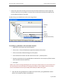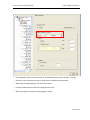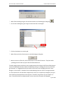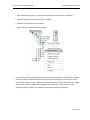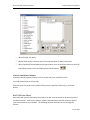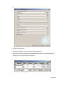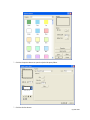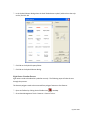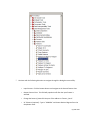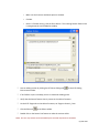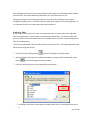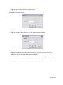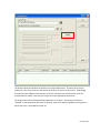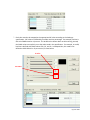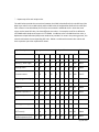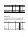
1
PLTS for ArcGIS - Nautical Solution
HAC Production Procedures
Contents
Introduction ___________________________________________________________________ 4
ArcMap Settings________________________________________________________________ 4
Toolbar Configurations __________________________________________________________________ 5
Maplex Label Engine ____________________________________________________________________ 7
Product Library_________________________________________________________________ 8
Setting up the Product Library permissions within an SDE environment ___________________________ 8
Setting up the Product Library users _______________________________________________________ 8
Configuring Product Library for HAC Production ______________________________________________ 9
Loading DNC VPF data into the Geodatabase _______________________________________________ 14
Adding New Product to Product Library ___________________________________________________ 17
Associating a geodatabase with an Product Instance _________________________________________ 19
Archiving DNC VPF data with product (optional)_____________________________________________ 20
Checking out a Product _________________________________________________________________ 20
Grid and Border Creation _______________________________________________________ 22
Grid Definitions (XML) examples _________________________________________________________ 23
AOI Origin Not in Lower Left (Optional) ____________________________________________________ 24
Checking the AOI Origin (Optional) _______________________________________________________ 25
Defining Grid Settings __________________________________________________________________ 26
Checking the Standard Parallel and Central Meridian (Optional) ________________________________ 26
Setting the Standard Parallel and Central Meridian __________________________________________ 28
Generate the UTM Grid (optional) ________________________________________________________ 28
Creating Grids for Charts with More than Four Sides (Optional) ________________________________ 36
Creating Grids for “Non-North Up” Panels (Optional) _________________________________________ 42
Creating Grids for Panels that Cross the 180° Meridian (optional) _______________________________ 43
Grid Edits (Optional) ___________________________________________________________________ 47
Add Grid Data (Optional) _______________________________________________________________ 52
Product and Document Settings __________________________________________________ 52
Chart Projection and Scale ______________________________________________________________ 52
Page Size ____________________________________________________________________________ 53
Updating Product Library _______________________________________________________________ 53
Activating Data Frames (Optional) ________________________________________________________ 56
Switching from Data to Layout View ______________________________________________________ 57
Remove Empty Feature Layers (Optional) __________________________________________________ 57
Table of Contents Organization (Optional) _________________________________________________ 58
Annotation ___________________________________________________________________ 59
PLTS for ArcGIS - Nautical Solution
HAC Production Procedures
Annotation Feature Class Setup __________________________________________________________ 59
Labels to Annotation Conversion _________________________________________________________ 61
Appending Annotation to Single Feature Class ______________________________________________ 63
Optimize Database Performance and Size __________________________________________________ 67
Review Unplaced Annotation ____________________________________________________________ 70
Add Missing Annotation (Optional) _______________________________________________________ 71
General Annotation Guidance ___________________________________________________________ 73
DNC/VPF Notes Check _________________________________________________________________ 73
Advanced Symbology __________________________________________________________ 77
Create Compass Rose Points ____________________________________________________________ 77
Flipping Buoy and Beacon Symbols (Optional) ______________________________________________ 83
Separation Area Symbology Setup (Optional) _______________________________________________ 87
Apply Visual Specifications ______________________________________________________________ 90
Change the Direction of the Light Flare and Traffic Separation Points ____________________________ 93
Symbolizing Reefs (Optional) ____________________________________________________________ 99
Embankment Symbol Adjustment (Optional) ______________________________________________ 104
Light Sector Creation Process ___________________________________________________________ 107
Quality Assurance & Quality Control _____________________________________________ 111
Background Images (Optional) __________________________________________________________ 112
Cartographic Finishing _________________________________________________________ 113
General Guidance for Annotation Cleanup ________________________________________________ 113
Symbology Edits _____________________________________________________________________ 114
Port Facilities Features ________________________________________________________________ 115
Masking ____________________________________________________________________ 115
Delete Unnecessary Masks _____________________________________________________________ 121
Page Layout _________________________________________________________________ 123
Layout View Setup ___________________________________________________________________ 123
Managing Elements __________________________________________________________________ 127
Add Surround Elements _______________________________________________________________ 129
Element Snapping ____________________________________________________________________ 130
Surround Elements List ________________________________________________________ 130
Simple Notes ________________________________________________________________________ 131
Notes Needing Edits __________________________________________________________________ 131
Surround Elements – Advanced _________________________________________________ 138
Note Information ____________________________________________________________________ 138
Scale Bars __________________________________________________________________________ 138
Source Diagram ______________________________________________________________________ 156
Exporting ___________________________________________________________________ 169
Color Separation _____________________________________________________________________ 174
Converting EPS file to PDF _____________________________________________________________ 180
Page 2 of 204
PLTS for ArcGIS - Nautical Solution
HAC Production Procedures
3rd Party Post export QA/QC ___________________________________________________________ 183
Archiving Products ____________________________________________________________ 186
Checking In Products to Product Library __________________________________________________ 186
Archiving Exported Files _______________________________________________________________ 189
Appendix A—Insets ___________________________________________________________ 189
Appendix B—Troubleshooting __________________________________________________ 196
Chart Export ________________________________________________________________________ 196
MXD Doctor Utility ___________________________________________________________________ 199
Invalid Product Configuration___________________________________________________________ 203
Compass Roses and VST _______________________________________________________________ 204
Page 3 of 204
PLTS for ArcGIS - Nautical Solution
HAC Production Procedures
Introduction
These production procedures guide you through all the basic steps required to produce a printready Nautical chart using VPF data. It provides the necessary steps to import data, symbolize it, and
finish a hard copy nautical chart. You should have a solid understanding of ArcGIS, Digital Nautical
Chart (DNC) VPF data, geodatabases, and projections. These procedures are also intended to be
used for creating Electronic products on demand (EPODs).
ArcMap Settings
The following ArcMap Extensions will be used for Production.
) Open ArcMap.
) Tools > Extensions… > Select the following:
o
Maplex: Provides an advanced label placement engine for ArcGIS.
o
PLTS Foundation Tools: Includes editing, import, export, and other tools. Most of
the tools used during the chart production process will come from the PLTS for
ArcGIS—Foundation extension.
o
PLTS MPS Atlas: Allows advanced map production capability.
o
PLTS Nautical Solution: Provides a variety of tools to produce spatial data for
hydrographic agency data models and specifications.
Page 4 of 204
PLTS for ArcGIS - Nautical Solution
)
HAC Production Procedures
Click Close.
Toolbar Configurations
It is highly recommended that the next steps be completed before chart production; however, it can
be done at any time during chart production depending on the necessity of the toolbars and the
amount of space on the computer screen.
In the last step, the user turned on the tool extensions so the tools could be used in ArcMap. The
next steps explain how to add the toolbars that contain the tools to the MXD.
NOTE: It is suggested that the Tools toolbar be placed away from the Layout toolbar. When in data view,
the Layout toolbar is inactive while the Tools toolbar is active. However, when in layout view, some of
Page 5 of 204
PLTS for ArcGIS - Nautical Solution
HAC Production Procedures
the tools on the Tools toolbar continue to remain active such as the Pan tool. This can create confusion
when working in layout view, since the Pan tool and the Layout Pan tool look similar. If the toolbars are
not already added to the MXD, it will be necessary to do so now.
) Go to the Tools menu and choose Customize. The Customize dialog box appears.
) The Toolbars tab should be active. There will be a check in the box next to the toolbar if it is
turned on.
) Click the check box next to the following toolbars to add them to ArcMap:
Page 6 of 204
PLTS for ArcGIS - Nautical Solution
HAC Production Procedures
o
Annotation: A core ArcMap toolbar that allows annotation editing.
o
Labeling: A core ArcMap toolbar used to modify the settings of the Maplex Label
Engine.
o
Layout: A core ArcMap toolbar that becomes active only when in layout view.
o
PLTS Editing: A PLTS for ArcGIS—Foundation toolbar with many of the core Foundation
editing tools.
o
PLTS Editing Advanced: A PLTS for ArcGIS—Foundation toolbar which has more robust
editing capabilities.
o
PLTS Editing Environment: A PLTS for ArcGIS—Foundation toolbar.
o
PLTS Grid Manager: A PLTS for ArcGIS—Foundation toolbar which is used during the
grid creation process.
o
PLTS Nautical DNC: The only PLTS for ArcGIS—Nautical Solution toolbar that is used
during chart production.
o
Representation: A core ArcMap toolbar that allows representation manipulation.
o
Standard: A core ArcMap toolbar that contains basic commands needed for using
ArcMap.
o
Tools: A core ArcMap toolbar that contains the basic tools for navigation within ArcMap
as well as other functionality.
) After verifying or adding the toolbars above, click the Close button to close the Customize
dialog box. These toolbars may be docked or moved, depending on the user's preference.
Maplex Label Engine
Maplex label engine supplies advanced automatic label placement functionality. Nautical charts rely
on Maplex to place the text on the charts in the most optimized location.
NOTE: This is a mandatory step. Failure to activate the Maplex Label Engine will alter the nautical feature
class layers.
) Click the Labeling drop-down menu on the Labeling toolbar and choose Use Maplex Label
Engine.
Page 7 of 204
PLTS for ArcGIS - Nautical Solution
HAC Production Procedures
Product Library
Note: For further information please refer to the Help menu and PLTS Desktop Help. Click on the Contents
tab and navigate to Managing maps and data with the product library, Getting started with the product
library, and An overview of the product library.
Product Library production workflow allows the user to store and organize their chart products as a
part of their production process. A single product may be checked out by an individual at any time
during production process in order to complete edits to the product before checking the edited
product into the product library for storage. If the user plans to produce and maintain products
over a long period of time than product library is the appropriate workflow.
Setting up the Product Library permissions within an SDE environment
Note: For further information please refer to the Help menu and PLTS Desktop Help. Click on the Contents
tab and navigate to Managing maps and data with the product library, Working with the product library,
Setting up the product library, and About product library permissions.
Within an SDE environment there are two different levels of permission settings, administrators and
users. The administrators have complete control over the product library structure, components,
and user permissions. These setting are accessible through ArcCatalog. To set up the product
library permissions within an SDE environment please refer to PLTS help.
Setting up the Product Library users
Note: For further information please refer to the Help menu and PLTS Desktop Help. Click on the Contents
tab and navigate to Managing maps and data with the product library, Working with the product library,
Setting up the product library, and Adding users to the product library.
The administrator has the ability to control the process of adding users, removing users and
assigning permissions to users within the product library. This process must be completed using the
administrator’s database connection. The administrator can create new accounts for the users who
will be accessing the product library and then apply their permissions once the individual is added.
The permissions levels that are available to the administrator are Not Available, Read Only, Check
In/Check Out and Edit level. To set up the product library users within an SDE environment please
refer to PLTS help.
Page 8 of 204
PLTS for ArcGIS - Nautical Solution
HAC Production Procedures
Configuring Product Library for HAC Production
Note: For further information please refer to the Help menu and PLTS Desktop Help. Click on the Contents
tab and navigate to Managing maps and data with the product library, Setting up the product library
database adding users to the product library or Setting up the product library with and SDE environment.
The product library example used in the HAC production procedures is based on a single user accessing
templates from the product library. For further information on configuring the product library to add
additional users or set up the product library in an SDE environment please refer to the help above.
The configuring of product library is only required once, if these steps have already been completed
they are not required for each new chart. The HAC Product Library database will contain four
product classes Approach, Coastal, General and Harbor, each with a template map document. Each
template has a preset list of the layers and symbols required to make the appropriate type of
product.
) Open ArcMap.
) Click Tools and choose Options.
The Options dialog box appears.
) Click Table of Contents Tab.
The Table of Contents tab appears.
) Scroll down the Table of Contents tabs window.
) Check Product Library check box.
) Click Ok.
) Click the Product Library tab.
The Data Management dialog box appears.
Page 9 of 204
PLTS for ArcGIS - Nautical Solution
HAC Production Procedures
) Click the cell next to Workspace.
) Click Workspace browse button.
The “Please browse to the location of the Product Library” dialog box appears.
) Navigate to the folder or SDE connection which the Product Library is located at.
) Select the Product Library database. If one does not exist, create a new a new geodatabase.
) Click Open. If prompted to upgrade, please select Yes.
) Click Ok.
The Data Management dialog box appears.
Page 10 of 204
PLTS for ArcGIS - Nautical Solution
HAC Production Procedures
) Click Ok.
) The Product Library appears.
) Right click on the “Product Library” node it the tree and click “New Solution”.
) Change the Name from “NewSolution” to “Nautical”
) Change Visible to True.
) Click OK.
) Right-click the “Nautical” solution and select “New Class” and fill out the following:
o Name: Approach.
o Alias: Approach.
o Description: Fill out a Description.
o Set Visibility to TRUE.
) Click on the + in front of Template to expand the template information.
Page 11 of 204
PLTS for ArcGIS - Nautical Solution
HAC Production Procedures
) Highlight and delete the “NewClass.mxd” as the File name.
) Click the small … (browse button) inside the File name location.
) Click the … (browse button) on the Browse For File dialog.
) Locate and select a template MXD and click Open.
) Enter a description.
) Click OK
) Repeat the process outlined above of added a new class and template MXD for the remaining
each product classes (Coastal, General, and Harbor).
) When completed the Product Library structure should look something like this:
Page 12 of 204
PLTS for ArcGIS - Nautical Solution
HAC Production Procedures
) Right-click on any of the product classes (Approach, Costal, General or Harbor) and click “New
Series”.
) Enter a name, alias and set visible to True. At least one series must exist under a product class. A
series is a way of subdividing a product class in to manageable pieces, typically based on
geographic extent.
Page 13 of 204
PLTS for ArcGIS - Nautical Solution
HAC Production Procedures
) Click OK.
) Repeat the steps outlined above to create additional series under the same product class or
different ones.
Loading DNC VPF data into the Geodatabase
) Open ArcCatalog
) Locate the appropriate scale geodatabase template (Approach.mdb, Coastal.mdb, General.mdb,
or Harbour.mdb)
) Select the geodatabase and right-click and choose Copy.
) Browse to a temporary folder location and paste the geodatabase template.
)
Right-click on the geodatabase template and choose Rename, enter the name of the Chart
being produced (i.e. 18704.mdb).
) Click Tools > Customize
) Click on the Toolbars tab, check PLTS, the PLTS toolbar is added.
) Click on the Commands tab, Under Categories select PLTS Import Export.
) On the right side of the Customize dialog, select Convert VPF Data to Geodatabase
) Drag and drop the command onto the PLTS toolbar.
) Close the Customize dialog.
) Click the Convert VPF Data to Geodatabase tool.
) Set the tool with the settings shown below, however ensure the Type of Scale is set
appropriately based on the chart being produced (Approach, General, Coastal, or Harbor):
Page 14 of 204
PLTS for ArcGIS - Nautical Solution
HAC Production Procedures
) Click Next>.
) Browse and select the folder for the DNC library (i.e. DNC13) for the VPF data path.
) Select library to import into geodatabase
Page 15 of 204
PLTS for ArcGIS - Nautical Solution
HAC Production Procedures
) Click Next>.
) Browse and select the chart geodatabase created earlier in a temporary folder location.
Page 16 of 204
PLTS for ArcGIS - Nautical Solution
HAC Production Procedures
) Click Next>.
) Review the summary information and click FINISH. This import process may take a few minutes.
) When asked to Review the log file, click Yes. Once done reviewing log, close the text file.
) Close ArcCatalog.
Adding New Product to Product Library
) In ArcMap add any existing shape file or feature classes to ArcMap which represent the
extents of the chart panels. For example you can use the Dqyarea feature class inside the
feature dataset inside the chart geodatabase.
) Select the feature which represents the charts Area of Interest (AOI)
Page 17 of 204
PLTS for ArcGIS - Nautical Solution
HAC Production Procedures
) On the Product Library tab right-click on the any of the newly added series and choose Batch
Import New Product. The Batch Import New Products dialog box appears.
) Click the Product drop-down and choose a field (i.e name) which will identity each
chart/products name.
) Keep the Repeating Product Values default option.
NOTE: If necessary, choose allow multiple instances per product. The Product Instance drop-down
becomes available to the user if this option is selected. Click on the field in which the user wants to use to
create the multiple instances.
) Click Ok.
NOTE: The Batch Import New Products can be performed on more than one chart at a time if required.
) The product features are created based on the AOI features selected.
Page 18 of 204
PLTS for ArcGIS - Nautical Solution
HAC Production Procedures
) If there are more than one AOI per instance they should be combined to create a single AOI.
Click the check box next to product’s instance. Start an edit session and use the merge tool to
join the adjacent features. Save edits.
Product Library tree should look similar to the image below.
Solution
Class
Series
Product
Instance
AOI (Area of Interest)
Associating a geodatabase with an Product Instance
) Right-click on the Instance and click Properties.
) Click on the + in front of Database to expand the database information.
) Click in the Location field and change it to File system.
) Click inside the File location text box and click the small … (browse) button.
) Browse to and select the chart geodatabase created earlier in the temporary folder location
which the DNC data was loaded into.
) Click Open.
NOTE: If you receive a message indicating the file is too large for Product Library or it cannot check in the
file at this time, the issue most likely is an existing lock on the file. Close ArcMap, remove any existing
locks on the database and the reopen ArcMap with a blank/new MXD and try again.
)
Now that the chart geodatabase is loaded into Product Library, the geodatabase created
earlier in the temporary folder can be deleted.
Page 19 of 204
PLTS for ArcGIS - Nautical Solution
HAC Production Procedures
Archiving DNC VPF data with product (optional)
) Using Windows browse and select the folder that contains the DNC library (i.e. DNC13) VPF
path.
) Compress (zip) the folder.
) Select the compressed file (zip file) and copy it.
) On the Product Library tab, select the product.
) Right-click and chose Manager Files.
) In the file manager dialog, right-click any of the blank area and chose Paste.
NOTE: The file is now archived and associated with a particular chart product inside Product Library. If
the file are needed again at a future date they can be accessed using the same tool.
Checking out a Product
Note: For further information please refer to the Help menu and PLTS Desktop Help. Click on the Contents
tab and navigate to Managing maps and data with the product library, Administering the product library,
Managing product library components, and Checking products in and out.
) Expand the Product Library tree if necessary.
) Right-click on one of the products and choose Check Out Product.
The Check Out dialog box appears.
) Click the browse button.
The Browse For Folder dialog box appears.
Page 20 of 204
PLTS for ArcGIS - Nautical Solution
HAC Production Procedures
) Navigate to the working folder location.
) Check on the Open check box.
) Click OK.
) The ArcMap save dialog box appears.
Page 21 of 204
PLTS for ArcGIS - Nautical Solution
HAC Production Procedures
) Click No, unless the document needs to be saved.
Note: The Product is now checked out of the Product Library, indicating and preventing other users from
make changes to the “official” copy of the map document and geodatabase, until checked back in by you.
) Select the Product Library tab in the TOC.
) Expand the tree view to see the AOI for the product instance.
) Click the check box to load the layer into ArcMap.
)
Right-click the AOI node in Product Library and click Zoom To. ArcMap will zoom to the
location of the chart.
)
Click on Tools > Customize.
)
Check on the Labeling toolbar, on the toolbars tab.
)
Close the Customize dialog.
) Click the Lock Labels button
, to stop the redrawing of labels. This will decrease the time it
takes to draw the labels as you navigate around the chart’s extent.
Grid and Border Creation
The following International Hydrographic Organization (IHO) INT 2 Grid styles are used Nautical
Chart production: E, F, G, H, J, K, L, and M. See INT 2 Chart Specifications of the I.H.O. (Borders,
Graduation, Grids and Linear Scales) for grid examples. Each letter designation above corresponds
to a specific chart scale range. For example, see table below (taken from INT 2 specs):
Page 22 of 204
PLTS for ArcGIS - Nautical Solution
HAC Production Procedures
NOTE: INT 2 E and F scale ranges have been modified for HAC purposes. So INT 2 E goes from 1 to 50,000
and INT 2 F goes from 50,001 to 100,000.
Grid Definitions (XML) examples
o
INT2_E_NorthEast_0-30000.xml: Interpreted as style E, the chart extents are in the northeast
hemisphere, and the scale range is 1–30,000.
o
INT2_E_NorthEast_30001-50000.xml: Interpreted as style E, the chart extents are in the
northeast hemisphere, and the scale range is 30,001–50,000.
o
INT2_F_NorthEast.xml: Interpreted as style F, the chart extents are in the northeast
hemisphere, and the scale range is 50,001–100,000.
o
UTM_Primary_25000-45000.xml: Interpreted as the UTM grid XML that has the purple color
and is used for charts with a scale range of 25,000–45,000.
o
UTM_Secondary_25000-45000.xml: Interpreted as the UTM grid XML that has the cyan color
and is used for charts with a scale range of 25,000–45,000.
Note: For charts that cross the prime meridian and/or equator:
o
INT2_E_Equator_East_1-30000.xml: Interpreted as style E, the chart extents cross the equator,
the chart is in the eastern hemisphere, and the scale range is 1–30,000.
o
INT2_E_PrimeMeridian_Equator_1-30000.xml: Interpreted as style E, the chart extents cross
the equator and the prime meridian, and the scale range is 1–30,000.
o
INT2_E_PrimeMeridian_North_1-30000.xml: Interpreted as style E, the chart extents cross the
prime meridian, the chart is in the northern hemisphere, and the scale range is
1–30,000.
Page 23 of 204
PLTS for ArcGIS - Nautical Solution
HAC Production Procedures
NOTE: Other XMLs can be interpreted in similar ways as described above.
Grids must be created for navigational purposes. The PLTS Grid Manager toolbar contains the tools
used to create and edit internal and external grids.
) Ensure that your PLTS MPS Atlas extension is turned on: Tools > Extensions and check PLTS MPS
Atlas, then Close.
) If necessary, add the Grid Manager toolbar to your ArcMap session. Click View > Toolbars > PLTS
Grid Manager. Dock it in a convenient location.
) Right-click the AOI feature in Product Library and click Select.
) From the Grid Manager toolbar, launch the Grid Creation Wizard
.
) Select the XML file appropriate for the chart (INT2_E, INT2_F, etc.). Make sure to choose the
XML based on whether it is in the eastern or western hemisphere
) Select the product database to save the grids into.
) Click next to GRD_ in the Dataset field and type a name “Grids”.
) For Extent, it should default to “Selected Polygon Features” but if not, select that option and
click Next.
NOTE: If the Grid Wizard gives you a warning message that the AOI Origin (from point) may not be lower
left , continue to section below, AOI origin not in lower left. If it does not, skip this section.
AOI Origin Not in Lower Left (Optional)
NOTE: If you do not have edit/write permission to your Product Library, you will not be able to conduct
the steps outlined below.
) Click No and close the Grid Creation Wizard.
) If necessary, add the PLTS Editing Environment toolbar View > Toolbars > PLTS Editing
Environment. Dock it to a convenient location.
Page 24 of 204
PLTS for ArcGIS - Nautical Solution
) Start an edit session
HAC Production Procedures
.
) If asked which folder or database do you want to edit data from, select the one which
represents the Product Library, and click OK.
) Select the AOI polygon if not already selected.
) From the Grid Manager Toolbar, select the Grid Origin Lower Left button.
) Click Yes to the dialog box with the warning message.
) Click Save Edits
) Stop editing
on the PLTS Editing Environment toolbar.
.
) Reselect the AOI polygon and click Grid Creation Wizard again to restart the process.
Checking the AOI Origin (Optional)
) Click the Edit tool
on the PLTS Editing toolbar.
) Using the Edit tool, double-click on the AOI feature to make the vertices appear.
) Click the Delete Vertices tool
on the PLTS Editing Advanced toolbar to make this tool active.
) Click and drag a box around the extra vertices and release the left mouse button. The vertices
present in the box will be deleted.
) Repeat these steps for each line segment that contains extra vertices until only the corner
vertices remain.
The starting vertex should always be in the lower left corner no matter which hemisphere the chart
is in. One way to check for this is to start an editing session, select only the AOI feature, click the
Sketch Properties button
, and when the Edit Sketch Properties menu appears, click the first
row in the menu. This should select the starting vertex. Another way to check is to start an editing
session and double-click on the AOI feature using the Edit tool button
found on the PLTS
Editing toolbar. The vertices should draw. If the red-square (ending) vertex is in the lower right
corner, the starting vertex would be in the lower left corner. If the red-square (ending) vertex or the
starting vertex is not in the proper location, create a new AOI to get the starting vertex in the lower
left corner and ending vertex (red square) in the lower right corner. Do this by creating a new AOI
Page 25 of 204
PLTS for ArcGIS - Nautical Solution
HAC Production Procedures
starting in the lower left corner and ending in the lower right corner going in a clockwise direction.
When creating the new AOI, snap to the current AOI.
) Click the PLTS Save Edits button and then the PLTS Stop Editing button on the PLTS Editing
Advanced toolbar.
Defining Grid Settings
) For Name, toggle the radio button to Name and type in a new name such as the name of the
panel or chart like <Panel_Name_A>, or use the Field and scroll to a field name from the
selected polygon feature.
) Set the scale option to the Custom radio button, and enter the chart’s scale (for example 25000)
and click Next.
) The Data Frame Rotation should remain as the default, Current Data Frame. Click Next.
o
Set the value of rotation to be the same as the panel OR
o
Select a new value for the rotation of the panel
o
See Help for more information on Data Frame Rotation
) For Conversion Options for the Primary and Ancillary Coordinate Systems, leave the defaults set
so that the Primary is set to Auto calculate, and the Ancillary is set to Accept the original
coordinate system. These can be changed at the summary page.
) Click Next.
) At the summary page, ensure that the correct XML is loaded and that the output database
location is correct.
) Check the Primary and Ancillary Coordinate systems, and update them if necessary:
Checking the Standard Parallel and Central Meridian (Optional)
The standard parallel and central meridian must be set on the grid for the chart to project correctly.
The first step is to find the standard parallel and central meridian values.
The standard parallel value can be found by going into the Dqyarea Attribute Table and looking at
the ref_lat attribute field.
Page 26 of 204
PLTS for ArcGIS - Nautical Solution
HAC Production Procedures
However, be aware that this value can sometimes be incorrect. To verify if it is correct, perform the
following (for northern hemisphere charts):
) Subtract the lower left latitude from the upper right latitude on the hard-copy chart.
) Divide the result by two.
) Add this result to the lower left latitude value.
) Convert this value to decimal degrees.
To verify if the ref_lat is correct for southern hemisphere charts, perform the following:
) Subtract the upper right latitude from the lower left latitude on the hard-copy chart.
) Divide the result by two.
) Add the result to the upper right latitude.
) Convert this value to decimal degrees and make the value negative.
The central meridian value cannot be found in the data, so it must be calculated manually. To
calculate the central meridian value for the western hemisphere, do the following:
) Subtract the upper right longitude on the chart from the lower left longitude on the chart.
) Divide the result by two.
) Add this value to the upper right longitude.
) Convert the results to decimal degrees (longitudes in the western hemisphere will be negative).
To calculate the central meridian value for the eastern hemisphere, do the following:
) Subtract the lower left longitude on the chart from the upper right longitude on the chart.
Page 27 of 204
PLTS for ArcGIS - Nautical Solution
HAC Production Procedures
) Divide the result by two.
) Add this value to the lower left longitude.
) Convert the results to decimal degrees.
Setting the Standard Parallel and Central Meridian
) In the tree view on the left, right-click the top-most node and select Primary Coordinate System.
) Click Select if you need to change the coordinate system.
) Click Modify if you need to make changes to the selected system.
) Click OK to apply and close the dialog box.
) Repeat steps to update/change the Ancillary Coordinate Systems if necessary.
) Click Create, keeping the default setting where each grid will be added to the Table of Contents
(TOC) as it is created.
) The grids will automatically be placed at the top of the TOC, be sure to keep them there.
) Click Close.
) In the table of contents, the EPT grid layer will need to be turned off. This is because these
points have a white color, which, when printed, will mask anything that is underneath them.
The layer ensures positional accuracy for annotation, as well as ends of lines, but do not need to
be visible on the chart. Uncheck the box for the EPT grid layer in the table of contents.
) Select the Product Library tab in the TOC.
) Expand the tree view to see the AOI for the product instance.
) Click off the check box to unload the layer from ArcMap.
) Save the MXD
using the name set by Product Library.
Generate the UTM Grid (optional)
If the chart has a scale between 1:25,000 and 1:300,000, a UTM grid must be created. The following
directions will aid the user in this process:
) Select the AOI extent again.
Page 28 of 204
PLTS for ArcGIS - Nautical Solution
) Click the Grid Creation Wizard button
HAC Production Procedures
on the PLTS Grid Manager toolbar.
The Grid Creation Wizard dialog box opens. The Storage area prompts the user to load an XML file
and save the edited XML into the user's geodatabase.
) In the Load area, click the Open File button
.
) Navigate to the location of the XML files.
) Select the XML file appropriate for the chart (e.g., UTM_East_25000-45000.xml). Make sure to
choose the XML based on whether it is in the eastern or western hemisphere.
) In the Save area in the Database field, click the Open File button
.
) Navigate to the location of the working geodatabase.
) Select the geodatabase and click OK to save the grid within that geodatabase.
o
In the Dataset field, notice that GRD_ is unavailable. GRD_ is the prefix given to every
grid created.
) Click next to GRD_ in the Dataset field and type a name that is meaningful for the XML (e.g.,
<chart number>_UTM).
) Click Next.
) For Extent, click Selected Polygon Features.
) Click Next.
o
The Name area prompts the user to either create a name for the grid or select a field
with a name already in it. In the Scale area, the user sets the scale of the chart so that it
creates the grid lines correctly.
) In the Name area, click the Field radio button; scroll down to and choose name in the right-hand
list.
) In the Scale area, click the Field radio button. Scroll down to and select scale in the right-hand
list.
Page 29 of 204
PLTS for ArcGIS - Nautical Solution
HAC Production Procedures
) Click Next.
) In the Data Frame Rotation area, make sure that Current Data Frame is selected and click Next.
This next panel has options for setting both the primary and ancillary coordinate systems.
) For Primary Coordinate System, click the Use data frame's projected coordinate system radio
button.
) For Ancillary Coordinate Systems, click the Auto calculate radio button.
Page 30 of 204
PLTS for ArcGIS - Nautical Solution
HAC Production Procedures
) Click Next.
o
It is important that the user review the grid creation properties before creating the
grid. First, verify that all data entered into the Grid Creation Wizard is correct.
) Right-click the XML on the Summary tab on the left side of the dialog box.
Page 31 of 204
PLTS for ArcGIS - Nautical Solution
HAC Production Procedures
) Check that the scale is set to the same scale of the chart, then click Primary Coordinate
System. The Spatial Reference Properties dialog box appears.
Page 32 of 204
PLTS for ArcGIS - Nautical Solution
HAC Production Procedures
) Click Select. The Browse for Coordinate System dialog box appears.
) Double-click the Projected Coordinate Systems folder.
) Double-click the UTM folder.
Page 33 of 204
PLTS for ArcGIS - Nautical Solution
HAC Production Procedures
) Double-click the WGS 1984 folder.
) Double-click the projection that matches the chart (e.g., WGS_1984_UTM Zone_17N.prj).
) Click the Add button.
) Check that the zone chosen is in the Name field on the Spatial Reference Properties dialog
box.
) Click OK to close the dialog box.
) A Grid Creation Wizard window appears. Click Apply to accept the default settings and close
the dialog box.
Page 34 of 204
PLTS for ArcGIS - Nautical Solution
HAC Production Procedures
) Click OK on the next window that appears.
) Click the Create button to create the UTM grid.
) Once the grid is created, click the Close button to exit the Grid Creation Wizard.
Page 35 of 204
PLTS for ArcGIS - Nautical Solution
HAC Production Procedures
) Edit the grid to make it chart specific.
Creating Grids for Charts with More than Four Sides (Optional)
After having completed the grid section above, follow these directions for modifying grids with
manual edits to match the chart extents that have more than four sides (“knock outs” or “doglegs”).
If your chart extent does not have more than four sides, you may skip this section.
) Reselect the AOI polygon in ArcMap if it’s not selected. Make sure it stays selected throughout
the following process.
) Open the Grid Designer
.
) In the tree view on the left, right-click on the topmost item (the name) and click Collapse.
) Select and expand Neatline01, right-click on it and click Collapse. Segments 01-Left, 02-Top, 03Right, and 04-Bottom should now be visible but collapsed; the other Neatlines are collapsed as
well.
Grid segments created by the Grid Manager need to start (ideally) in the lower left, and the
segments count up in a clock-wise fashion. All XML files provided with PLTS assume to have only 4
sides. Once this is reached, the last XML segment is repeated until all AOI segments are covered. In
the case of an AOI having more than 4 sides, segments that have the same orientation need to be
copied and pasted. See example image below.
Page 36 of 204
PLTS for ArcGIS - Nautical Solution
HAC Production Procedures
The blue numbers represent the actual number of segments. The red numbers represent the order
in which the segments need to be copied and pasted: starting from the lower left and rotating clockwise around the extent.
) Start from the lower left corner and number the segments on a scratch piece of paper similar to
the image above. In this example, segments 1, 2, and 3 need to be copied and reordered. The
final order for this example will be 1, 2, 1, 2, 3, 2, 3, and 4. It is expected that the chart created
will most likely not match this example, and will need to be adjusted accordingly.
) In the Grid Designer, right-click on the first segment and click Copy.
Page 37 of 204
PLTS for ArcGIS - Nautical Solution
HAC Production Procedures
) Right-click on Neatline01 and click Paste. Segment05-Left is added to the bottom of the list. It
may be necessary to select Neatline01 and collapse it after each time you paste or move a
segment.
) Right-click on Segment05-Left, and click Order > Move Up. Notice it is renumbered and is now
called Segment04-Left.
) Repeat the above step (move up) until this second Left segment is below the first Top segment
so that segments 1, 2, and 3 are Left, Top, Left.
Page 38 of 204
PLTS for ArcGIS - Nautical Solution
HAC Production Procedures
) Right-click on the Top segment and click Copy.
) Right-click on Neatline01 and click Paste. Segment06-Top is added to the list.
) Right-click on Segment06-Top, and click Order > Move up. Continue moving this Top segment up
until it is below the second Left segment. The order should now be Left, Top, Left, Top, Right,
and Bottom.
) Repeat the copy/paste steps for the Top segment, and move it below the Right segment.
) Repeat the copy/paste steps for the Right segment, and move it up until it is after the last Top
segment. The final order should be Left, Top, Left, Top, Right, Top, Right, and Bottom, with a
total of 8 segments. Again, please note this is for this example only and other situations may
require modifications.
Page 39 of 204
PLTS for ArcGIS - Nautical Solution
HAC Production Procedures
) Once the segments have been copied, pasted, and re-ordered, click the top node in the Grid
Designer. In the example shown, it would be the chart number.
) Click the Create button.
Page 40 of 204
PLTS for ArcGIS - Nautical Solution
HAC Production Procedures
) The program will ask you if you want to override what was already created. Click Yes.
) Zoom in and pan/scan (use tools from the Tools toolbar) the newly updated grid to ensure that
the corrections were successful. If any discrepancies are noted, open the Grid Designer again to
make corrections. If necessary, plot out a paper version of the grid for verification of its
accuracy.
Page 41 of 204
PLTS for ArcGIS - Nautical Solution
) Save the product MXD
HAC Production Procedures
.
Creating Grids for “Non-North Up” Panels (Optional)
All INT2 Grid XML files are designed for panels that have north at the top of the chart. If the panel
you are producing is not “north up”, you need to ensure the angle of the annotation meets the
desired appearance. Annotation rotation can be controlled using the Grid Designer or edited
interactively after the grid is created. Keeping that in mind, if the annotation is to remain parallel to
the grid lines, no adjustments are necessary, provided the input remains as “Current Data Frame”
and the data frame has been rotated. However, if the chart you’re making needs to have the
annotation remain parallel to the page, and not the data frame, then adjustments need to be made
to the XML file in the Grid Designer. Follow the below steps as an example of how to rotate the data
frame and maintain the text parallel to the page, not the grid lines.
) Open the product MXD in ArcMap.
) If necessary, zoom to the extent of the chart.
) If necessary, load the AOI polygon that was originally used to create the grids.
) Select the AOI polygon. Be sure that the polygon remains selected throughout the process.
) If necessary, add the Data Frame Tools toolbar and/or the PLTS Grid Manager toolbar to the
ArcMap session. Click View > Toolbars > Data Frame Tools, and dock it in a convenient location.
) On the Data Frame Tools toolbar, enter the numeric value of degrees rotated (clockwise from
North). Be sure to rotate it the exact same number of degrees.
Note: You can also click the Data Frame Rotation button, click-and-drag the mouse to rotate the Data
Frame so that the AOI polygon is now oriented in the same manner in which it will be viewed. For more
information, see help under Data Frame Rotation.
) It may be necessary to ensure that the polygon begins with the lower left corner; refer to that
section.
) Open the Grid Designer
from the PLTS Grid Manager toolbar.
) In the tree view, select each section’s annotation.
o
Change the option for rotation from Use Text Symbol Angle to Rotate to Data Frame.
o
Repeat as necessary for all the annotation.
) Click the top node of the tree (the grid name) and click Create.
Page 42 of 204
PLTS for ArcGIS - Nautical Solution
HAC Production Procedures
) Minimize the designer window, zoom in, pan and scan (use tools from the Tools toolbar) to see
if the desired results were achieved.
) If other charts will be produced with similar annotation changes, this XML can be saved to a
shared location and given a logical name so that it can be used again.
o
If necessary, click the top node again.
o
Save the grid to XML with a logical name.
Creating Grids for Panels that Cross the 180° Meridian (optional)
Typically features are split when crossing the 180th meridian. However, to create grids the span the
180 a single area of interest feature with single (part) geometry is required. The steps below
describe how that area of interest feature is created.
) Start a new ArcMap document.
) In ArcMap, select the Product Library tab in the TOC.
) Expand the tree view to see the AOI for the product instance.
) Click the check box to load the layer into ArcMap
) Select the Display tab in the TOC
) Access the data frame properties of the active data frame and select the Coordinate System tab.
) Under the Select a coordinate system browse to Predefined > Projected Coordinate Systems >
World > Mercator (world).
Page 43 of 204
PLTS for ArcGIS - Nautical Solution
HAC Production Procedures
) Select Mercator (world) and click the Modify…button
) Enter a Central Meridian value of 180 and click OK.
Page 44 of 204
PLTS for ArcGIS - Nautical Solution
HAC Production Procedures
) Click OK on the Data Frame Properties to apply the change.
NOTE: The AOI that was added to the data frame should now appear in the center of data view and two
parts of the AOI should now be adjacent.
) Right click the layer that displays the AOI (layer name many vary however format will appear
similar to: “Nautical::Chart::CGD17::c514”) and choose Data > Export Data
) In the Export Data dialog Use the same coordinate system as the data frame and browse to a
location to create the output shape file.
Page 45 of 204
PLTS for ArcGIS - Nautical Solution
HAC Production Procedures
) Click OK, when asked if you want to add the exported data to the map as a layer click Yes.
) Remove the Product Library AOI layer from TOC.
) Start an edit session on the Shape file source just created (Export_Output)
) Select the AOI feature.
) On the PLTS Editing Advanced toolbar click the “Simplify selected features” command.
NOTE: The feature will be merged into a single part feature and can be used for grid creation. If desired
the Shape file can be maintained for future use and processing inside Product Library using its file manger.
) On the PLTS Grid manager toolbar click the Grid Origin Lower Left command. If prompted to
update the feature, click Yes.
) Stop editing and save the edits.
) Start a new ArcMap document; don’t save change to exist document.
) Add the edited shape file back to ArcMap, select the feature and create the grid using the Grid
Creation Wizard.
NOTE: The MXDs used to create the AOI are not required to be kept, once the grid is created and saved in
the database it can be added to any ArcMap document using the Add Grid Data command.
Page 46 of 204
PLTS for ArcGIS - Nautical Solution
HAC Production Procedures
Grid Edits (Optional)
Most grids will need to have further editing done to them. There are several different kinds of edits,
some of which require the user of PLTS Grid Designer to adjust grid values, and there are some that
require manual editing.
An example of this is when working on a chart that does not have perfectly vertical or horizontal
sides. Notice in the image below that the grid ticks are not perfectly horizontal or vertical as they
should be. Tick marks are always drawn perpendicular to the neatline. Therefore, with a chart
similar to the one used in this example, the grid will have to be edited to make the tick marks
perfectly horizontal or vertical.
PLTS Grid Designer is the main method used to edit grids. Since edits vary from chart to chart, this
section will focus on basic PLTS Grid Designer use.
It is important that the user edit the grid first in PLTS Grid Designer. Once a final version is made
through PLTS Grid Designer, manual edits should be made. However, if the user needs to go back
Page 47 of 204
PLTS for ArcGIS - Nautical Solution
HAC Production Procedures
and rerun PLTS Grid Designer on the same grid, all manual edits will be overwritten and will need to
be redone. This is because the grid is created from a static XML file.
) Click the PLTS Grid Designer button
on the PLTS Grid Manager toolbar.
) In the left-hand column on the Grid Designer dialog box, click the title of the grid to activate it.
Notice in the Grid Properties area on the right that many of the fields are now populated with
information.
) To associate the feature on the chart with the item in Grid Designer, right-click on anything in
the left column of the Grid Designer dialog box and choose Select Component.
Page 48 of 204
PLTS for ArcGIS - Nautical Solution
HAC Production Procedures
This will select the different items in the PLTS Grid Designer on the map as they are clicked on the
Grid Designer dialog box.
) Make all necessary edits.
) If the gridline interval needs to be modified, click Gridline01 and set the proper interval under
the Interval tab. Gridline01 should represent longitude. To check, click the Direction tab and
ensure that it is set to North-South. The interval can be set in degrees, minutes, seconds, or
percentage.
Page 49 of 204
PLTS for ArcGIS - Nautical Solution
HAC Production Procedures
) Click Gridline02 and set the proper interval. Gridline02 should represent latitude. To check,
follow the same instructions as step 5, except that it should be set to East-West.
) When finished editing the grid, click the top title again.
) Click the Create button to create the new grid on the chart.
) When prompted to overwrite the existing grid, click Yes.
Page 50 of 204
PLTS for ArcGIS - Nautical Solution
HAC Production Procedures
) When finished editing the grid, click the Save button on the Grid Designer dialog box
.
) On the Save As dialog box, give the grid a new name that is meaningful.
) Click the Save button to save the grid.
) When finished, click the Close button on the Grid Designer dialog box.
) Make sure to turn off the CLP, PNT, and EPT layers in the table of contents. They have white
symbology that will mask any layers that fall underneath them.
The other editing option would be to start an editing session by clicking the PLTS Start Editing button
on the PLTS Editing Environment toolbar and deleting, moving, or changing the various parts of the
grid manually. It is suggested that this be used as a last resort, when changing the items in Grid
Designer is not an option. Examples of this include deleting excess tick lines or moving annotation.
It is also important to note that when a Dqyarea has a slant (it is not perfectly rectangular), the grid
ticks will always be perpendicular to the Dqyarea. Therefore, the grid ticks may also appear at a
slant. These will have to be edited manually, as this cannot be corrected in Grid Designer.
Page 51 of 204
PLTS for ArcGIS - Nautical Solution
HAC Production Procedures
Add Grid Data (Optional)
The Add Grid Data button allows the user to add an existing grid to the current ArcMap table of
contents with the correct symbology. If a grid dataset has already been created in the database and
found on the
needs to be added to the table of contents then click the Add Grid Data button
PLTS Grid Manager Toolbar. When the Add Grid Data window pops up click the browse
button
and when the ‘Database location for grid’ window appears navigate to the dataset
that has the grid. Single click on the dataset that is needed then click the OK button. After clicking
OK the user will be returned to the Add Grid Data window. Check the box next to the grid name that
is needed within the section Grid Names > Names (MAPIDs), uncheck the Zoom to grid(s) box, and
then click the Add button. The grid should automatically be added to the table of contents. Click the
Close button on the Add Grid Data window once the grid is added to the table of contents.
Note: Do not use the Add Data button
to add the grid into ArcMap. If this is done, the grid will
appear in the table of contents and incorrect symbology will be displayed for the individual feature
classes.
Product and Document Settings
Chart Projection and Scale
This step automatically re-projects and scales the panels. It is important to set this information
correctly, especially when it comes to creating and adjusting annotation placement and other
cartographic edits. The shapes of features and text placement need to be in the chart’s projection
and scale to ensure the desired placement is achieved, to reduce feature conflicts. This step will
override the current projection and scale of the MXD in favor of what was defined for the grid of the
chart.
NOTE: There are three locations where the projection and scale information for a chart’s panel can be set.
The grid, the data frame(s) in the MXD and the Product Library. The parameters defined in these three
locations should be the same. The process defined below ensures both the grid and data frame are
synchronized. When the product is checked back into the Product Library, Product Library will check to
ensure they match.
) Open the product MXD, if not already open.
) From the Grid Manager toolbar, click the Grid Layout View button
.
If more than one
grid is loaded into ArcMap’s table of contents select the one that has the chart’s primary
coordinate system.
Page 52 of 204
PLTS for ArcGIS - Nautical Solution
HAC Production Procedures
) Click OK to the warning dialog box.
) ArcMap automatically updates your grids, projection, standard parallel and meridian, and
switches to the Layout View.
) Right click on the Data Frame and select Reference Scale > Set Refereance Scale.
) Optional step: If you do not want to set your page size now, toggle back to the Data View, and
Save the product MXD
chart.
. You will need to do this however, before you print your hard-copy
Page Size
The page size has to be modified based on the scale of the chart and its geographic extent. It is
important to set this up now, so that it will not conflict with Layout features in future steps.
) From the menu toolbar in ArcMap, click File > Page and Print Setup.
) Uncheck the box Use Printer Paper Settings inside the Map Page Size box.
) In the Standard Sizes drop down inside the Page box, select the size which fits the chart (for
example, ANSI E).
) Choose the orientation of the chart as either Portrait or Landscape.
)
If nothing matches the chart measurements in the Standard Sizes box, enter the width and
height of the paper into their respective fields in the Page box.
) Select Centimeters from the Width and Height drop down boxes.
)
Click OK.
) Using the Select Element tool on the Drawing toolbar, click and drag the data frame to a location
on the page. More detail placement will be address later.
) Save the MXD
.
Updating Product Library
Note: For further information please refer to the Help menu and PLTS Desktop Help. Click on the Contents
tab and navigate to Managing maps and data with the product library, Administering the product library,
Managing product library components, and Checking products in and out.
Page 53 of 204
PLTS for ArcGIS - Nautical Solution
HAC Production Procedures
) Close ArcMap and restart it, to remove any applications locks on the file or database.
) Select the Product Library tab in the TOC in ArcMap.
) Expand the tree view to see the product.
) Right-click on the product and select Check in.
) You may receive a message indicating that there are conflicting values in the MXD you are about
to check in with the product properties as specified in Product Library. For example, the data
frame’s scale, reference scale, rotation or its spatial reference may have different values. Review
these values in both the MXD and Product Library to see which is correct, and choose the
appropriate option (typical it is to Update Product Library with map properties).
Page 54 of 204
PLTS for ArcGIS - Nautical Solution
HAC Production Procedures
) Click OK.
) Decide if you want to overwrite the current version, or to increase the minor draft version
number.
) Enter in comments of what you’ve done and why you’re checking it in/keeping it checked out.
) If you plan on continue working on your product (yes), make sure you check the box “Keep
checked out” so that you can resume making changes and edits to your product.
) When finished, click OK.
Page 55 of 204
PLTS for ArcGIS - Nautical Solution
HAC Production Procedures
) Click OK.
Activating Data Frames (Optional)
This is an optional step. These instructions should be used when a chart requires multiple data
frames in ArcMap. For example, a chart may have panels, plans, or insets that require a second or
third data frame. If the chart being produced only has one data frame, that data frame will already
be active.
) Right-click the main data frame in the table of contents.
) Choose Activate. The data frame label becomes boldface. This indicates that it is activated.
Page 56 of 204
PLTS for ArcGIS - Nautical Solution
HAC Production Procedures
Switching from Data to Layout View
This step may be completed several times throughout the chart production process. When edit
feature in the database it best one in data view, when working on the page layout, printing and
export, the layout view. It is recommended that the user become extremely familiar with this
process.
To make the extent of the chart display correctly in layout view, it is necessary to set a fixed scale
equal to the reference scale when the user switches from data view to layout view. This should
always be performed when switching from data view to layout view. Switching to layout view can be
perform at any point by clicking on the Grid Layout Tool
.
Remove Empty Feature Layers (Optional)
Removing empty feature layers makes the table of contents more manageable. The following
directions will aid the user in completing this process:
NOTE: Do not remove the CompassRoseP layer file at any time.
) Click the Remove Empty Feature Layers button on the PLTS TOC Manager toolbar.
Although this will remove empty feature layers, it will not remove group layer titles, only the +/- sign
next to the layer titles.
To remove the group layer titles:
) Right-click the empty group layer and click Remove.
Page 57 of 204
PLTS for ArcGIS - Nautical Solution
HAC Production Procedures
Table of Contents Organization (Optional)
For features to display properly, the table of contents in ArcMap needs to be organized correctly.
The order listed below, from topmost layer to bottommost layer, should be the proper arrangement
of the feature layers in the table of contents.
o
GRD_<chart number>_UTM (if chart contains a universal transverse Mercator [UTM] grid)
(top)
o
GRD_<chart number>_INT2
o
CompassRoseP
o
All_Annotation
o
Ecrtext
o
Mask layers
o
All points according to alphabetical order
o
All lines according to alphabetical order
o
All polygons according to alphabetical order (except those listed below)
o
EcrArea
o
ReefA
o
ForeshoA
o
SepartnA
o
Hydarea
o
Dqyarea (bottom)
Page 58 of 204
PLTS for ArcGIS - Nautical Solution
HAC Production Procedures
Annotation
Annotation Feature Class Setup
Currently, the MXD should have all the layers added and all the labels turned on that are necessary.
The labels may overlap in places and could be covered by lines. It is important for the labels to be
legible on the chart, therefore, the labels must be converted to annotation, adjusted if necessary,
and masked. This section focuses on that process. Before converting to annotation, double-check
that the Hydline labels are not too close together. If they are, the labels will need to be adjusted
accordingly. Also, ensure that the reference scale is set correctly for the All_Annotation and Ecrtext
feature classes. To check and modify the reference scale, follow these steps:
) Open ArcCatalog.
) Navigate to the geodatabase for your chart.
) Expand the geodatabase in the Catalog tree.
) Expand the feature dataset in the Catalog tree (DNCH, DNCA, DNCC, DNCG).
) Right-click the All_Annotation feature class and select Properties.
) Click the Annotation tab and examine the current reference scale. If incorrect, click the
Change button and set to the chart scale.
) Click OK on the Reference Scale window.
Page 59 of 204
PLTS for ArcGIS - Nautical Solution
HAC Production Procedures
) Click OK on the Feature Class Properties window.
) Click Yes on the new window that appears, asking are you sure you want to apply the new
reference scale.
) Repeat this procedure for the Ecrtext feature class.
Page 60 of 204
PLTS for ArcGIS - Nautical Solution
HAC Production Procedures
) Close ArcCatalog.
Labels to Annotation Conversion
NOTE: Ensure that all layers to be converted to annotation are turned on before completing the following
steps.
) Start ArcMap and reopen the chart mxd (File > 1<chart name>).then right-click the the main
data frame that stores the layers in the table of contents and select Convert Labels to
Annotation.
Use the following options in the Convert Labels to Annotation dialog box:
o
Store Annotation: In a database.
o
Create Annotation For: All features.
o
Convert unplaced labels to unplaced annotation: Checked.
o
Reference Scale: 1:<chart scale>.
Page 61 of 204
PLTS for ArcGIS - Nautical Solution
HAC Production Procedures
o
Feature Linked column: Uncheck all. Do a batch uncheck by unchecking the first layer in the
list, then scrolling down to the bottom, pressing the Ctrl key and unchecking the last layer.
All the check marks disappear.
o
Append column: Uncheck all. Use the Ctrl key in the same manner as above to do a batch
uncheck.
o
Annotation Feature Class column: Leave default values.
) Click the Convert button. Each feature class will have its own annotation feature class added to
the table of contents.
) If a warning is received indicating that the annotation feature class name already exists, rename
it in the list by appending a “2” to the entry in the far right column.
Page 62 of 204
PLTS for ArcGIS - Nautical Solution
HAC Production Procedures
Note: This process may take a few minutes, once completed annotation feature classes will be added to
the table of contents and the labels turned off.
Appending Annotation to Single Feature Class
To make editing of annotation easier, as well as organization of the table of contents more
manageable, it is suggested that one annotation feature class be used to house all the annotation
for the chart. To do this, the annotation must be appended to that single annotation class called
All_Annotation. To append all of the annotation for the chart into one feature class, the Append
Annotation Feature Classes tool in ArcToolbox must be used.
) While in ArcMap, click the ArcToolbox icon
.
) Go to Data Management Tools > Feature Class > Append Annotation Feature Classes.
) The Append Annotation Feature Classes window appears.
Page 63 of 204
PLTS for ArcGIS - Nautical Solution
HAC Production Procedures
) For the Input features text box, click the Browse button
and navigate to inside the
working feature dataset. All the annotation feature classes should become visible.
) To select all annotation feature classes, select the first one, press the Shift key on the
keyboard, and select the last annotation feature class. Unselect Ecrtext by holding down the
Ctrl key and selecting Ecrtext. Including Ecrtext in the append will cause duplication of the
Ecrtext features on the chart.
Page 64 of 204
PLTS for ArcGIS - Nautical Solution
HAC Production Procedures
) Click Add to close the Input features window.
) On the Append Annotation Feature Classes window, click the Browse button
Output Feature Class field.
next to the
) Select the All_Annotation annotation feature class.
) Click Save to return to the Append Annotation Feature Classes dialog box. The Reference Scale
field will automatically populate itself with the chart's scale after the Output feature class is set.
This may take a few moments.
Page 65 of 204
PLTS for ArcGIS - Nautical Solution
HAC Production Procedures
Many of the options will become unavailable.
) Check the Create a single annotation class box.
) Click OK.
) Once the process is finished running, click Close on the small window that pops up. The
annotation is now appended into one feature class.
Since the annotation is appended, it is no longer necessary to have the individual annotation feature
classes in the table of contents in ArcMap. The following steps will take the user through the
process of removing them:
) Select the first annotation feature class at the top of the table of contents.
) Hold down the Shift key on the keyboard.
) Select the last annotation feature class in the table of contents.
) Ensure All_Annotation and Ecrtext is not selected (Ctrl click to remove).
) Right-click and click Remove.
Page 66 of 204
PLTS for ArcGIS - Nautical Solution
HAC Production Procedures
All the annotation feature classes disappear from the table of contents.
) Save change to you MXD.
Optimize Database Performance and Size
To enhance redraw performance in ArcMap, the All_Annotation feature class can be projected to
match the on-the-fly projection of the chart. To convert the All_Annotation feature class to a
Mercator projection, follow the steps below:
) Click on the Grid Designer command on the Grid Manager toolbar.
Page 67 of 204
PLTS for ArcGIS - Nautical Solution
HAC Production Procedures
) Select the grid (top node) in the Grid Designer dialog.
) Click the Coordiante System button under Primary Coordiante System grouping, the coordinate
system of the grid, and in turn the chart is displayed.
) Click Save As.
) Browse to the file system location of the map document and database.
) Enter a name for the coordiante system file and click Save, this will create a file on the local
system that will be acccesed in a future steps.
) Click Cancel to close the Spatial Reference dialog.
) Click Close to close the Grid Designer dialog.
) Open ArcToolbox.
) In ArcToolbox, click Data Management Tools > Projections and Transformations > Feature >
Project.
) In the Input Dataset or Feature Class field, navigate to your geodatabase and select the
All_Annotation feature class.
The Input Coordinate System (optional) field will automatically be populated and unavailable.
) The Output Dataset or Feature Class field will also be automatically populated and will default to
your current geodatabase. The default naming convention will be All_Anno_Projected. If
desired, change the name of the new projected All_Annotation feature class.
) Click the
button to the right of the Output Coordinate System field to select the projection.
) On the Spatial Reference Properties window, click the Select button and navigate to file system
location of the map document and geodatabase where the coordinate system file was saved
previously.
) Select the PRJ file that was created as one of your Favorites earlier.
) Click OK.
) Leave the Geographic Transformation box empty and click OK.
Page 68 of 204
PLTS for ArcGIS - Nautical Solution
HAC Production Procedures
) The tool will run for several seconds.
) Remove the unprojected All_Annotation feature class and add the projected feature class.
) Save Change to the MXD and close ArcMap to remove any locks on the database.
) Open ArcCatalog to remove the extra annotation feature classes from the geodatabase.
) Click on Tools>Options.
) On the Contents tab, check on Feature Type under the “Which standard columns do you want to
show in Details View?”
) Click OK.
) Location your chart database in the tree view and select the feature dataset, all feature classes
will be displayed in the right of ArcCatalog.
) Click on the Feature Type column to soure based one feature type.
) Select all annotation feature classes, except All_Annotation_Projected and Ecrtext.
Page 69 of 204
PLTS for ArcGIS - Nautical Solution
HAC Production Procedures
) Delete the selected feature classes (insure All_Annotation_Projected and Ecrtext are not
selected, this may take a few minutes.
) Close ArcCatalog.
Review Unplaced Annotation
During the conversion process, the option to convert unplaced labels to annotation was used.
Unplaced annotation is text that was overlapping and therefore dropped from the map. In most
cases, this is the desired effect, but occasionally there may be unplaced annotation that needs to be
displayed.
) Open ArcMap and the chart mxd.
) Start and edit session; click the Unplaced Annotation button
on the Annotation toolbar.
) In the Show drop-down list, choose <Visible Annotation Layers>.
) Uncheck the box next to Visible Extent. Click the Search Now button.
) Review the list of unplaced annotation and determine if any significant text such as Sounding
labels or Light Legends are unplaced. Unplaced annotation from Depth Curve labels and other
insignificant features can likely remain that way.
) Add the annotation to the chart by right-clicking on it in the Unplaced Annotation dialog box and
selecting Place Annotation.
Page 70 of 204
PLTS for ArcGIS - Nautical Solution
HAC Production Procedures
Add Missing Annotation (Optional)
This is optional because not all charts may have missing annotation. Missing annotation, however,
is not the same thing as unplaced annotation. If annotation is missing, use the following steps to
add the annotation:
) Start an editing session by clicking the PLTS Start Editing button
Environment toolbar.
on the PLTS Editing
) Click the PLTS Target tab in the table of contents.
) Select the All_Annotation feature class on the PLTS Target tab.
Page 71 of 204
PLTS for ArcGIS - Nautical Solution
HAC Production Procedures
) On the Annotation toolbar, type in the text that needs to be added in the Text box.
) From the Symbol drop-down list on the Annotation toolbar, select the style for the text.
) Click the Construct Horizontal Annotation tool
on the Annotation toolbar.
) Click on the chart where the annotation needs to be added. The text should appear on the
chart.
) If the annotation just added needs to be corrected (or any annotation needs to be corrected
in general), select it with the Select Annotation tool
on the Annotation toolbar.
) Right-click the annotation string and choose Attributes from the menu that appears.
) Edit the text of the newly added annotation in the text box on the Annotation tab on the
Attributes window, if necessary. The font and text size can be adjusted as well.
Page 72 of 204
PLTS for ArcGIS - Nautical Solution
HAC Production Procedures
) When finished, click Apply.
) Repeat these steps as necessary until all missing annotation is added to the chart.
) When completely finished adding missing annotation, click the PLTS Save Edits then the PLTS
Stop Editing buttons on the PLTS Editing Environment toolbar.
General Annotation Guidance
Annotation describing water features, such as oceans and rivers, should be in italic.
Land and cultural features are not italic.
Some text sizes may need to be increased if they portray a significant feature (e.g., the Pacific
Ocean).
DNC/VPF Notes Check
Most notes will relate to information that needs to be put in the surrounds at the end of the chart
production process. Some notes, however, relate to individual layers and will need to be placed
next to those features as annotation. The following steps will help take the user through this
process:
Page 73 of 204
PLTS for ArcGIS - Nautical Solution
HAC Production Procedures
The Notes Editor tool—found on the PLTS Nautical DNC toolbar—must be used to look at the
notes.rat features of the chart.
) Start by setting the selectable layers. On the PLTS Editing Environment toolbar, click the Set
Selectable Layers button
.
) Click the Select All button on the Set Selectable Layers window that opens.
) Close the window by clicking the Close button.
) Make sure all the layers required for the chart are turned on in the table of contents.
) Click the Notes Editor button on the PLTS Nautical DNC toolbar.
Click the Select Features With Attached Notes tool within the Notes Editor window that opens.
NOTE: Although the standard Select Features button and the DNC Select Features With Attached Notes
button look identical, using the standard selection button does not select features with notes. The Select
Features With Attached Notes tool must be used.
Page 74 of 204
PLTS for ArcGIS - Nautical Solution
HAC Production Procedures
) Drag a box around all features on the chart to select all the data. All feature classes with
notes attached will appear inside the Notes Editor left column menu.
) Scroll down the list to see which layers have notes.
As stated before, some notes will be added as a surround. An example of something that would
need to be added as annotation is "Radio tower X has a height of 102 meters." Using annotation,
the user would place a "(102)" next to the tower specified.
If unsure to which object the note refers, click the note in the left-hand column. It will flash on the
map.
For directions on how to add annotation, see section on , Add Missing Annotation.
Page 75 of 204
Advanced Symbology
The Visual Specification set of tools (VST) allows the user to make more advanced symbolization of
features using feature class representations. VST is used to depict compass roses, light flare
rotation, buoy/beacon orientation, and traffic separation directional points. The following steps will
guide the user through the process of using VST to "finish" the symbology for these features.
) Copy the ePODS_M.style file into the path C:\Program Files\ArcGIS\Styles. This style
contains many additional symbols that are used during the chart production process.
NOTE: Ensure ePODS-M style file is properly installed before continuing.
Create Compass Rose Points
The following steps get the user started on VST use:
) On the hard-copy chart, find and take note of the coordinates of the existing compass roses
or the locations of where the compass roses will need to be.
NOTE: Compass rose placement—Whenever practical, a point shall be selected for compass rose
placement in every quadrant of a nautical chart subject to double folding. Chart size, shape of land areas,
and density will affect the number of points selected. Sufficient points shall be selected to ensure that all
navigable waters are within 18 inches of a compass rose.
) Measure to see how large the compass roses are on the hard-copy chart. These sizes must
be used when creating the chart.
) Make note of the coordinates of any additional compass roses that need to be added from
step 2 above.
NOTE: If possible, compass roses should not obstruct anything on the chart, especially features that are
the same color as the compass rose.
The following steps will guide the user through the process of creating the compass rose points on
the chart in ArcMap:
) If the CompassRoseP layer file is not loaded in the table of contents then click the Add Data
button
in ArcMap.
) Start an editing session by clicking the PLTS Start Editing button
Environment toolbar.
on the PLTS Editing
) Click the PLTS Target tab on the Table of Contents window.
Page 77 of 204
) In the Target field, select the CompassRoseP point feature class.
) In the Fields and Values columns on the PLTS Target tab in the table of contents, click the 5
Inches - 5 value next to the Diameter field.
) From the drop-down menu that appears, choose the correct diameter of the first compass
rose to be digitized.
) Click in the Values column for the Location field. Select the name for the location of the
compass rose on the chart.
Page 78 of 204
NOTE: Even if the default value is correct, click the drop-down menu and select the correct values.
The fields will turn blue to show that they have not yet been applied to the data that is to be
digitized.
) Click the Apply button on the PLTS Target tab in the table of contents to apply the attributes
to the feature that is going to be digitized.
NOTE: If the Apply button is not clicked, the attributes will not be linked to the feature to be digitized and
the attributes will have to be input manually on the PLTS Selection tab in the table of contents.
Page 79 of 204
NOTE: To verify that the attributes have been applied, the text for those attributes that were changed
turns from blue back to black.
) On the PLTS Editing toolbar, click the Create New Features In Target Layer button
.
NOTE: This automatically changes the cursor to a point instead of an arrow. The user should notice that
the sketch tool has also become activated when the Create New Features In Target Layer button is clicked
.
) In the ArcMap display window where the chart is drawn, click the location on the chart
where the compass rose needs to be placed. A point appears in this location.
) Repeat steps above for each compass rose that needs to be created. The attribute values
for the diameter and location of each compass rose should be adjusted accordingly since
each compass rose will be different.
) When finished creating all compass roses, click the PLTS Save Edits and then PLTS Stop
Editing buttons on the PLTS Editing Environment toolbar.
Open the attribute table
by right clicking on the CompassRoseP layer file in the table of contents and selecting Open
Attribute Table to verify that features have been added correctly.
The World Magnetic Model (WMM) Calculator will automatically populate the Magnetic Declination
and Variance (called Drift in the Calculator) in the attribute table for the compass rose points. The
following steps will show the user how to use the tool:
) Click the ArcToolbox icon
in ArcMap.
) Within ArcToolbox, navigate to PLTS Foundation Tools > Magnetic > Magnetic Calculator.
Page 80 of 204
) Double-click Magnetic Calculator to open it. The tool is robust and may take a minute to open.
) When the window appears, enter the information as shown below:
o
Input Feature Class or Raster Dataset: CompassRoseP (use the drop-down menu to
select it directly from the MXD).
o
Linear Unit: Meters.
o
Altitude: Click the Double radio button, and enter "0" as the value.
o
Date: Double-check that the date listed is the current date.
o
Output Declination Field (optional): The word "Declination" must be entered.
o
Output Annual Drift Field (optional): The word "Drift" must be entered.
o
Leave all other fields as default values.
Page 81 of 204
) Click OK to run the tool.
) Once the tool finishes running, click Close on the progress box.
) Open up the attribute table of the CompassRoseP point feature class to double-check that
the Declination and Drift fields were populated.
Page 82 of 204
Flipping Buoy and Beacon Symbols (Optional)
Buoys do not need to be flipped unless they are obstructing another black object such as a sounding.
Most charts will not require buoy flipping. In the event that buoys need to be flipped, follow the
directions below to use VST:
) Make sure the BuoybcnP layer file is in the ArcMap table of contents.
) Open the attribute table for the BuoybcnP object.
For example, if the buoy that needs to be flipped is a pillar buoy with a CCC of green, the user would
right-click on the BuoybcnP – Buoy Top Mark Pillar/Other/Unk Green CCC sublayer in the table of
contents and select Open Attribute Table.
) Scroll to the Symbol_Flip field in the attribute table.
on the PLTS Editing
) Start an editing session by clicking the PLTS Start Editing button
Environment toolbar.
Below and on the next page are two charts. One is the Base Letter with Base Picture chart. This
shows the four different bases the user can choose from when flipping the symbol; the letter A
stands for a spar buoy, B is an open buoy, C is a safe water buoy, and D is a filled buoy.
The second chart is called Topmark Number with Topmark Picture. The number above the topmark
picture is what the user would associate with that picture. For example, 1 is an East Mark topmark
and 2 is an Isolated Danger topmark.
Base Letter with Base Picture
A
B
C
D
Page 83 of 204
Topmark Number with Topmark Picture
1
2
3
4
5
6
7
8
9
10
11
12
13
14
15
16
17
18
19
20
21
22
Page 84 of 204
) For the BuoybcnP symbol to appear correctly on the chart using VST, the user must specify
which base symbol and which topmark (if any) should be used. The user specifies this in the
Symbol_Flip column of the BuoybcnP attribute table.
Here are examples of how the user might fill in this column with the appropriate symbol:
) The BuoybcnP that needs to be flipped has a Spar (A) base and an East Mark (1) topmark.
A
1
B
2
C
3
D
4
5
Therefore, the user would enter "A1" into the Symbol_Flip field.
Page 85 of 204
) The BuoybcnP that needs to be flipped is simply a safe water buoy.
A
B
C
D
Therefore, the user would use the chart above to see that a safe water buoy is C. The user would
type "C" in the Symbol_Flip column.
) The BuoybcnP that needs to be flipped is a filled buoy with a Diamond Over Ball topmark.
A
B
C
D
Page 86 of 204
21
22
Therefore, the user would enter "D21" into the Symbol_Flip field in the BuoybcnP attribute table.
NOTE: The letter must always come before the number for VST to understand which symbol to use. If
done the other way around, VST will fail.
) Find the symbol values using the charts above enter the letter followed by the number for
the symbol into the Symbol_Flip column.
) Repeat the step above until all symbols that need to be flipped have a value in their
Symbol_Flip field.
) Save edits and stop editing by clicking the PLTS Save Edits and then the PLTS Stop Editing
buttons on the PLTS Editing Environment toolbar.
Separation Area Symbology Setup (Optional)
Not all charts have SepartnP features. Therefore, this step is not necessary for all charts.
In the event that the user does have the SepartnP feature class, VST will need to be used to
symbolize the features correctly. It is important that the user follow all of the directions, or VST will
not symbolize the features correctly or at all.
Page 87 of 204
) In ArcMap, make sure that the SepartnP feature class has been added to the MXD.
) Click the PLTS Start Editing button
editing session.
on the PLTS Editing Environment toolbar to start an
) Right-click the SepartnP feature class and choose Open Attribute Table.
) Scroll all the way to the right in the attribute table.
) If the RotateAngle field is empty, right-click in it and select Field Calculator.
) When the Field Calculator window opens, in the Fields box, double-click dof.
) Click OK on the Field Calculator window.
The RotateAngle field should populate with the values from the dof field. It is necessary to do this
because VST will need those values to determine the rotation of the symbol. The dof field is of data
Page 88 of 204
type double, while VST will only read rotation values from a field type of float. The RotateAngle field
is a float field.
) In the ArrowType field, enter the type of arrow needed to be symbolized. The list of
available types is below.
NOTE: These types must be typed in correctly, or VST will not symbolize them correctly! Use copy/paste
for best results.
o
Straight Solid
o
Straight Dashed
o
Curved Right Solid
o
Curved Right Dashed
o
Curved Left Solid
o
Curved Left Dashed
NOTE: The name "Solid" indicates that the arrow symbol has solid lines creating it. The name "Dashed"
indicates that the arrow symbol has dash marks creating it. The name "Right" indicates that the
arrowhead points to the right, depicting a clockwise rotation of traffic. The name "Left" indicates that the
arrowhead points to the left, depicting a counterclockwise rotation of traffic. See Chart No. 1, section M,
page 52 for examples of these symbols.
) Once all fields are entered, click PLTS Save Edits and then PLTS Stop Editing on the PLTS
Editing Environment toolbar.
The SepartnP feature class is now ready to have VST run on it.
Page 89 of 204
Apply Visual Specifications
The following steps outline the last items that need to be completed for compass rose, light flare,
SepartnP (optional), and BuoybcnP (optional) symbol creation.
) Stop editing, if still in an editing session, open ArcToolbox, if it is not already open, by
clicking on the ArcToolbox icon
in ArcMap.
) Navigate to PLTS MPS-Atlas Tools > Visual Specification > Calculate Visual Specifications.
) Double-click Calculate Visual Specification to open the tool.
) From the Input Layers or Feature Classes drop-down menu, select the CompassRoseP point
feature class and the LightsP – Flare sublayer. If the chart has a SepartnP feature class, select
that from the drop-down menu as well. If the chart has BuoybcnP flips, select the BuoybcnP –
VST Flip sublayer from the BuoybcnP Group layer.
) Click the Browse button next to the Visual specification table location field.
) On the Visual specification table location window, navigate to the location of the working
geodatabase, select it, and click Add.
Page 90 of 204
In the Visual Specifications field, the following options should become available:
o
CompassRose
o
LightsP
o
SepartnP
o
BuoybcnP
) Check the option boxes next to the CompassRose and LightsP choices. If the chart has a
SepartnP feature class, check the SepartnP choice. If the chart has BuoybcnP flips, check the
BuoybcnP choice.
) The Calculate Visual Specifications window should look similar to the one below:
Page 91 of 204
NOTE: BuoybcnP and SepartnP are optional. Never check the TreeA option.
) Click the OK button. It will take some minutes to process.
) When the process is complete, click Close on the processing window that appears.
NOTE: It may be necessary to re-run VST on BuoybcnP – VST flip, SepartnP, CompassRoseP, or LightsP –
Flare. This would occur if the user made changes after the initial VST has been run. If this is the case then
the user should use the Drop Visual Specifications tool located in ArcToolbox > PLTS MPS-Atlas Tools >
Visual Specification > Drop Visual Specifications. Fill out the menu with ONLY the feature class that VST
would need to be processed again. For example, if BuoybcnP needs to have VST run on it again then
choose BuoybcnP – VST Flip for Input, the current database for table location, and check the BuoybcnP
box within the Visual Specifications section, then click OK. After the process has finished, run the
Calculate Visual Specifications tool on the BuoybcnP - VST flip feature class.
Page 92 of 204
) Ensure the compass rose is being labeled with the magnetic information.
) Convert the labels to annotation on the CompassRoseP layer, with the Append option to the
All_Annotation_Projected feature class.
Change the Direction of the Light Flare and Traffic Separation Points
Changing the direction of the light flares and traffic separation points is simple. Currently, the light
flare points in a northwest direction.
NOTE: The easiest way to rotate light flares and traffic separation points is to use the Rotate Tool
located on the Representation toolbar. To use the Rotate Tool start an editing session, click on the Select
Tool
button that is located on the Representation toolbar, select the feature that needs to be
rotated, then click the Rotate Tool button
and rotate the feature in any direction.
Page 93 of 204
For another option for the light flare direction to be changed, the user will need to add the number
of degrees the flare needs to move in the FlareAngle field in the LightsP-Flare attribute table.
For example, if the user wants to make the flare point southeast, simply enter "180" into the field,
and the flare will point southeast.
) Start an editing session by clicking the PLTS Start Editing button
Environment toolbar.
on the PLTS Editing
) Open the LightsP - Flare attribute table by right-clicking the layer in the table of contents and
selecting Open Attribute Table.
) In the FlareAngle field, enter the desired degree change.
) Close the attribute table.
) Click the PLTS Save Edits button and then the PLTS Stop Editing button on the PLTS Editing
Environment toolbar.
) Refresh the map.
Page 94 of 204
The flare automatically adjusts for the angle change.
The following values in table specify the desired flare direction and the value that needs to be
entered into the LightsP - Flare attribute table:
Table 10-1
Direction
Value
Direction
Number
N
45
S
225
NNE
68
SSW
248
Page 95 of 204
NE
90
SW
270
ENE
113
WSW
293
E
135
W
315
ESE
158
WNW
338
SE
180
NW
0
SSE
203
NNW
23
To change the angle of the traffic separation point, the user must change the value entered in the
RotateAngle field of the SepartnP attribute table.
) If not already in an editing session, start one by clicking the PLTS Start Editing button on the
PLTS Editing Environment toolbar.
) Right-click the SepartnP layer in the table of contents and choose Open Attribute Table.
) For the point that needs to have the value changed, enter the correct angle value into the
RotateAngle field. Use table below to find the correct value for the direction of the symbol.
) When finished entering all the angles, save the edits and stop editing by clicking the PLTS Save
Edits button and then the PLTS Stop Editing button on the PLTS Editing Environment toolbar.
) If the symbols do not automatically adjust to the correct angle, try refreshing the map. If that
does not work, double-click the SepartnP feature class in the table of contents.
) On the PLTS Calculated Representations tab, uncheck and recheck the Update Feature Class(es)
option.
) Click OK on the Layer Properties window. The symbology adjusts accordingly.
Table 10-2
Direction
Value
Direction
Number
N
0/360
S
180
NNE
23
SSW
203
Page 96 of 204
NE
45
SW
225
ENE
68
WSW
248
E
90
W
270
ESE
113
WNW
293
SE
135
NW
315
SSE
158
NNW
338
All symbols turn clockwise, regardless if the arrow points to the right or to the left. For example, the
picture below shows curved symbols with both right-pointing arrows and left-pointing arrows at 0°,
90°, 180°, and 270°. By using the visual below, the user can figure out which angle the arrow should
have. The angle of the traffic separation points can also (instead of using the rotate tool) be changed
in the SepartnP attribute table by simply right-clicking on the SepartnP layer file in the table of
contents, choosing Open Attribute Table, and inputting an angle in the rows under the RotateAngle
column.
Page 97 of 204
Right Curved
Left Curved
0°
90°
Page 98 of 204
Symbolizing Reefs (Optional)
Not all charts have reef features; check the ReefA feature class before proceeding. For reefs to be
displayed properly the overlapping section with the shoreline must be removed. This process is
accomplished with a series of geoprocessing tools.
) Inside of ArcMap, click the ArcToolbox icon
to open ArcToolbox.
) Go to Data Management Tools > Features > Feature To Line.
) Continue with the following directions to navigate through the dialog box successfully:
Page 99 of 204
o
Input Feature: Click the browse button and navigate to the ReefA feature class.
o
Output Feature Class: Click the browse button and navigate to the ReefL_Carto
feature class.
o
XY Tolerance (optional): Type in "0.0001" and choose Meters from the drop-down
menu.
o
Make sure the Preserve attributes option is checked.
o
Click OK.
o
Once it's finished running, click the Close button.
) Open the attribute table for the EcrArea feature class.
) Using the Select by Attributes under Options button select all land features with the query
example below.
Page 100 of 204
) Close EcrArea attribute table.
) In Toolbox go to Analysis Tools > Overlay > Erase.
Page 101 of 204
) Enter the following values:
o
Input Features: ReefL_Carto.
o
Erase Features: EcrArea.
o
Output Feature Class: <some location> ReefL_Carto_Erase.
o
XY Tolerance: 0.0001 Meters.
Page 102 of 204
) If the new ReefL_Carto_Erase feature class was added to ArcMap’s table of contents,
remove it.
) Access the Properties of the ReefL_Carto layer, select the Source Tab.
) Click the Set Data Source button and brose and select the ReefL_Carto_Erase feature class.
Page 103 of 204
) Click OK.
Now only the section of the reefs that is over water is displayed in the ReefL_Carto layer as a line
symbol.
) Save changes to your MXD.
Embankment Symbol Adjustment (Optional)
Depending on the location of the chart, there may or may not be embankments. If there are the
scale of the chart and the DNC data source can affect how the symbol is shown. There are two
embankment symbols one; one for large-scale charts and one for scale charts. Depending on the
chart, either symbol can be used to increase legibility. To decrees the sizes of the embankment
symbol use the steps below:
) Locate and expand the Lcrline Group 10K layer.
) Click once on the Use=Unknow symbol to open the Symbol Selection dialog.
Page 104 of 204
) Click the Save button to add the symbol to your personal style file.
) In the dialog that appears enter in the following information.
) Click OK.
) Click OK on the Symbol Selection dialog to close this window.
) Locate and expand the EmbankA layer.
) Click once on the DB090 symbol to open the Symbol Selection dialog.
Page 105 of 204
) Click the Properties button to open the Symbol Property Editor.
) Click the Outline button.
Page 106 of 204
) In the Symbol Selector dialog select the Small Embankment symbol (add to the to the style
earlier) and click OK.
) Click OK on the Symbol Property Editor.
) Click OK on the Symbol Selector dialog.
Light Sector Creation Process
Light sectors need to be edited to symbolize correctly. The following steps will take the user
through that process:
The SectorA polygons need to be converted from polygon features to line features.
) Open ArcToolbox by clicking the ArcToolbox icon
in ArcMap.
) Go to Data Management Tools > Features > Feature To Line.
Page 107 of 204
) Continue with the following directions to navigate through the dialog box successfully:
o
Input Feature: Click the browse button and navigate to the SectorA feature class.
o
Output Feature Class: This field will populate itself after the input feature is
selected.
o
Change the SectorA_FeatureToLine part of the address to "SectorL_Carto".
o
XY Tolerance (optional): Type in "0.000001" and choose Decimal degrees from the
drop-down menu.
Page 108 of 204
o
Make sure the Preserve attributes option is checked.
o
Click OK.
o
Once it's finished running, click the Close button. The resulting SectorL feature class
is now geometries and is added to ArcMap.
) Start an editing session by clicking the PLTS Start Editing tool
Environment toolbar.
on the PLTS Editing
) If ArcToolbox is open in ArcMap, close it to maximize drawing space.
) Verify that the SectorL feature class is present in the table of contents.
) On the PLTS Target tab on the table of contents, set Target to SectorL_Carto.
) Click the Edit tool
on the Editor toolbar.
) Double-click on the SectorL line feature to make the vertices visible.
NOTE: The user may need to set the selectable layers such that only SectorL is selectable.
Page 109 of 204
) On the Editor toolbar, click the Splits Linear Feature tool
.
) Click on a corner vertex to split the line feature there.
) Verify that the split was made by clicking on one of the lines to the right or left of the vertex.
) Double-click again on the SectorL line feature to make the vertices visible. Continue splitting
the line feature at all corner vertices or locations where there will need to be a change
between SectorL colors.
) Once all splits are made, right-click the SectorL feature class in the table of contents and
select Open Attribute Table. The Color column will be used to symbolize the SectorL feature
class.
) For each line, click the box in the Color field. A drop-down menu becomes available. The
color choices available are as follows: blue (B), red (R), green (G), misc. (Misc), orange (O),
violet (V), white (W), and yellow (Y).
NOTE: Misc should be used when a color is not present and only requires black dashed lines.
) Once all the attribution changes have been made, click the PLTS Save Edits button and then the
PLTS Stop Editing button on the PLTS Editing Environment toolbar.
Page 110 of 204
) Close the attribute table. By adding the color values exactly as above, the arc portions of the
sector will be symbolized with the proper colors in the following steps:
) Turn off both the SectorL and SectorA feature classes by right-clicking the check marks next to
their names in the table of contents.
) Click the Add Data button
on the Standard toolbar.
) Navigate to the location of the layer files on the computer.
) Click the SectorL_Carto layer file.
) Click OK. The layer file is added to the table of contents, but the data source needs to be set.
) Click the red exclamation mark next to the SectorL_Carto layer. The Set Data Source dialog box
opens.
) Navigate to the location of the SectorL feature class and select it.
) Click Add to close the Set Data Source dialog box. The SectorL_Carto layer appears on the chart
correctly symbolized.
Quality Assurance & Quality Control
) Plot out a scaled version of your chart.
Page 111 of 204
) Review the chart for areas of conflict, overprint and over-crowding, specifically for text
placement and representation overrides and the position and correctness of the surrounds.
Write on the page margins what steps need to be followed.
) Once the chart has been thoroughly examined, identify the same features on screen, and make
the necessary changes to the data and/or layout.
Background Images (Optional)
If there is the need to put a rectified TIFF (.tiff) image in the background of the MXD, a transparency
will need to be applied to the polygon layers in the chart so that the TIFF image can be seen through
the layers.
) Move the TIFF to the top of the table of contents.
) Right-click the TIFF and select Properties.
) On the Layer Properties window, click the Display tab.
) On the bottom left corner of the Display tab, set the transparency between 50 and
60 percent. (This value can be adjusted according to user preference.)
Page 112 of 204
Cartographic Finishing
General Guidance for Annotation Cleanup
o
Water features: Italicize annotation that is associated with water features.
o
Geonames: Adjust size and placement of important geonames (e.g., Pacific Ocean).
o
Hydro features: Occasionally, depth curve labels will either need to be removed or added. As
mentioned earlier, never move sounding depth annotation.
o
Navigation features: Adjust annotation placement for aids to navigation that require it such as
overlapping or poorly placed light legends. Light flares may also need to be rotated; VST can be
utilized. Also, ensure that all light and buoy annotation is outside of dredged channels.
o
Relief features: Occasionally the chart may depict a triangulation point that does not have its
own attribute in DNC (they are collected as relief points). If this is the case, a representation
would have to be created.
It is necessary to make sure annotation does not overlap, especially if it relates to a sounding.
Sounding and bottom characteristic annotation should never be moved from its original locations. If
sounding or bottom characteristic annotation is overlapped by another feature, the other feature
must be adjusted.
Annotation can overlap lines if the colors are different. For example, black annotation can overlap
purple limit lines but not a black route line. If the same colors overlap, the annotation will need to
be masked.
The steps below will guide the user in the event that annotation must be moved:
) Click the PLTS Start Editing button
) Use the Edit Annotation tool
on the PLTS Editing Environment toolbar.
on the Annotation toolbar to select an item of annotation.
) Drag the annotation to a better placement location.
) Once all annotation changes are made, click the PLTS Save Edits and then PLTS Stop Editing
buttons on the PLTS Editing Environment toolbar.
Page 113 of 204
Edits regarding the annotation text string should be made using the core Attributes button added in
previous steps. See section Add Missing Annotation, for more information on this.
Changing annotation text and moving annotation may need to be repeated as the chart goes
through the QA/QC process. Annotation edits will make up the majority of the finishing process, so
it is important that the user understands how to edit annotation.
Symbology Edits
It may not be necessary for every chart, but occasionally there are symbols where the alignment
affects navigation safety. One example is an Anchoring Prohibited limit. The Anchor symbol and
tick marks need to face inward toward the area. Examples of lines that often need to be flipped are
limits and embankments.
To fix this example problem, the user will have to manually flip the line. The following directions will
aid the user through the process:
) Click the PLTS Start Editing button
on the PLTS Editing Environment toolbar.
) Make the feature that needs to be edited selectable by clicking the PLTS Set Selectable Layers
button
on the PLTS Editing Environment toolbar.
) Click the Clear All button on the Set Selectable Layers window.
) Scroll down to the feature that needs to be edited and select it by checking the box next to
it.
Page 114 of 204
) Click the Edit tool
on the Editor toolbar to select it.
) Double-click on the line feature that needs to be flipped so that the vertices are visible.
) Temporarily add the PLTS Editing Advanced toolbar to the session by right-clicking in the
gray space and selecting it from the toolbar list that appears.
) Click the Flip button to flip the line.
) When finished editing, click the PLTS Save Edits and then the PLTS Stop Editing buttons on the
PLTS Editing Environment toolbar.
Port Facilities Features
Adjust annotation size and placement of port facilities. A common issue is that port features have
both lines and areas, which can cause duplicate labels to be placed. Duplicate labels will need to be
deleted. The following directions explain how to do this:
) Click the PLTS Start Editing button
) Click the Edit Annotation button
on the PLTS Editing Environment toolbar.
on the Annotation toolbar.
) Click on the duplicate piece of annotation to select it.
) Right-click and click Delete.
) When all duplicate labels are deleted, click the PLTS Save Edits and then the PLTS Stop Editing
buttons on the PLTS Editing Environment toolbar.
Masking
Once annotation editing is completed, it is necessary to mask the annotation. Masking uses a
polygon feature class around the annotation to "mask" features and provide improved chart
readability.
Page 115 of 204
In the event there is a need to move annotation after the masking process, both the annotation and
the mask that surrounds it will have to be moved.
It is important to note that while a polygon masking feature class will be created in this process, it is
suggested that only annotation be masked using this feature class. If additional features need to be
masked outside the Annotation feature class, additional feature outline mask feature classes should
be made for every instance.
) Ensure that you are not in an editing session.
) Click the ArcToolbox icon
in ArcMap.
) Navigate to Cartography Tools > Masking Tools > Feature Outline Masks.
) Follow these directions on the dialog box:
o
Input Layer: All_Annotation feature class (use the drop-down arrow and not the Browse
button to select the annotation layer).
Page 116 of 204
o
Output Feature Class: Navigate to the location of the feature dataset and give it a name
like Anno_Mask.
o
Reference Scale: Should be unavailable and set to the chart's scale.
o
Calculation coordinate system will be set because the annotation was reprojected.
o
Margin: Enter ".7" in the first box and leave the default Points from the drop-down
menu.
o
Mask Kind: CONVEX_HULL.
o
Create masks for unplaced annotation: ALL_FEATURES.
o
Transfer Attributes (optional): Leave as the default.
) Click OK to run the masking process.
) When the tool finishes running, click Close.
Page 117 of 204
There are a few modifications to the mask feature class that need to be made for it to function
properly.
) In the table of contents in ArcMap, click the fill symbol of the mask layer to open the Symbol
Selector window.
) On the left-hand side of the dialog box should be various colors displayed for the user to choose
from. Choose the option named Hollow.
Page 118 of 204
) On the right side, change Outline Color to No Color.
) Click OK to close the Layer Properties dialog box.
) Click the data frame to select it in the ArcMap table of contents.
) Right-click it and select Advanced Drawing Options.
Page 119 of 204
) At the top of the window, check the option for Draw using masking options specified below.
Page 120 of 204
) In the Masking Layers column, select the Anno_Mask feature class.
) In the Masked Layers column, check all of the line feature class boxes except any of CoastL
or LimbndyL layers.
) Do not select any lines that are purple on the chart, which usually includes limit lines. Do
make sure to select the interior GLN lines.
) When finished checking all the correct boxes, click OK to close the window. The masks
should create a buffer between the annotation and lines on the chart.
Note: Is recommended to turn off masking when it is not required, and only enable it before printing and
exporting to ensure faster draw types.
Delete Unnecessary Masks
Occasionally a chart may have too many masks, which will cause redrawing to slow. Unnecessary
masks include those around a piece of annotation that does not touch any line object. Do not
delete any masks whose annotation touches a line. To delete masks, follow the directions below:
Page 121 of 204
) Start an editing session by clicking the PLTS Start Editing button
Environment toolbar.
on the PLTS Editing
) On the PLTS Editing Environment toolbar, click the Set Selectable Layers button
.
) Make sure that only the annotation masking feature class is selectable. Click Close when
finished.
) Zoom to a section on the chart where annotation does not cover lines.
) Use the selection tool to select the masks.
) Click the
on the standard menu or the delete on the keyboard to remove the masks.
) Repeat as needed, deleting any unnecessary masks.
) When finished, click the PLTS Save Edits button followed by the PLTS Stop Editing button on
the PLTS Editing Environment toolbar.
Page 122 of 204
Page Layout
During the following steps, the user will be adding and customizing surrounds on the chart. Not all
surrounds listed may be needed on every chart, as variations occur from chart to chart.The user
must be in layout view to add surrounds.
Layout View Setup
The layout view needs to be set up for surround placement.
) Turn off all layer in ArcMap’s table of content (TOC) except the Grid grouped layers (starting
with a “GRD”). This will speed up the draw when working in the page layout, as the
geographic data does not need be edited any more.
on the Grid Manager toolbar. If more than one grid is loaded
) Click the Grid Layout tool
into ArcMap’s table of contents select the one the has the chart’s primary coordinate
system.
Note: Now that you are in Layout view be sure to navigate (pan and zoom) using the Layout toolbar
controls, the other navigate commands will change the scale and extent of the chart.
) Add a guide on one of the rulers by clicking on the ruler.
) Right-click on the guide just added and click Options.
Page 123 of 204
) On the Options window, click the Layout View tab.
) Check all of the boxes in the Appearance section except Stretch contents when window is
resized.
) Check the Show box.
) Choose Centimeters from the Units drop-down menu.
) Choose 0.1 cm from the Smallest Division drop-down menu.
) Check the Guides box in the Snap elements to section, and leave all the other boxes
unchecked.
) Set Snap Tolerance to 0.1 cm (equivalent to 1 mm).
Page 124 of 204
) Click OK to exit the Options dialog box.
Since surrounds will be placed according to the a particular border or surround style sheet, it is
important that the user have these documents available before adding the guides. Guides will
generally be placed at 1 mm, 2 mm, and 5 mm away from the outermost grid segment line of the
chart and will run parallel to this border. It is suggested that the user begin in the upper left corner
of the chart and work clockwise from corner to corner, adding guides as necessary. It is also
suggested that the user zoom in to the area where the guides are being added so that millimeter
divisions on the side rulers are easily visible.
Page 125 of 204
) Once the guide options are set and the documents necessary for guide placement are
obtained, guides are ready to be placed.
) Click on the ruler in layout view to add a guide. This will set a blue ruler guide in view.
) Repeat this step for every guide that needs to be added to layout view.
) In the event that a guide is placed incorrectly, do the following:
o
Pause the mouse pointer over it until the double-sided mouse arrow becomes visible.
o
Left-click the guide.
o
Drag it to the correct location.
One way of making sure the guides are the correct distance apart is by checking the distance with
the measurement pop-up window:
) Click and hold a guide. In the upper left-hand corner of layout view, a box should appear
stating the location measurement of the guide.
For example, if the user can visibly tell the ruler sits at 13.6 cm, the box would read
13.6 Centimeters. This can then be used to double-check the measurements to make sure the
guides are 1, 2, or 5 mm apart.
Page 126 of 204
If the guides do not show at any time, go to the View menu and select Guides. If at any time the
guides need to be turned off, go to the View menu and deselect Guides.
Managing Elements
Once elements are place they can be managed using the elements tab.
) Click Tools> Options select the Table Of Contents tab to enable the tab.
) Scroll through the list can check on Elements.
Page 127 of 204
) Click OK.
) Click on the Elements tab at the bottom of the table of contents.
) Right click on any element in the list to access commands like locking/unlocking and the
element properties.
) Once the data frame is positioned, it is highly suggested that is locked. Locate all the data
frames (globe), right click and select Lock Elements. This will prevent unintended moving or
adjusting of the element.
Page 128 of 204
Add Surround Elements
Once all the guides are in their correct locations, surround elements can be added. The following
steps will take the user through this process:
) Open up Database Elements from Insert > PLTS > Database Element
) Click the Browse button to navigate to the location of the Elements.mdb database or the
Product Library database if the elements are stored with the products.
) Once found, click it, and click the Select button to close the Select Workspace dialog box.
) In the bottom left column there are several different choices to choose from such as
Aeronautical and Defense.
) Double-click Nautical.
) Double-click HAC.
) Double-click Charting. A list of various elements appears.
Page 129 of 204
) Scroll down the list to find the element that is needed, click it, and click Insert. Repeat for
every element that is required for the particular chart.
Element Snapping
The purpose of the guides is to aid in the proper placement of elements by allowing the elements to
snap directly to them. However, unless the element has a premade border around it, the element
will have to be nudged so that the text falls directly on the guide. Only those elements with a
premade border can simply snap into position.
To nudge elements, make sure the element (and only the element) is selected. Then use the up,
down, left, and right arrow keys on the keyboard to nudge it in the right direction.
Elements can also be nudged by right-clicking them, scrolling to Nudge, and choosing the desired
direction.
Surround Elements List
This section describes the various surrounds and how to edit them.
Page 130 of 204
Not all these surround elements will be necessary for every chart because each is different. The
hard-copy chart is the best guide for deciding which notes to place. All notes that exist on the hardcopy chart should be added to the MXD; however, the values may need to be adjusted. Data will
also need to be checked for additional notes. Use the information in the subsection titled Notes
Check in section 9.0, Annotation, as a guide for this process.
Simple Notes
The following notes simply need to be inserted and placed on the chart: This may be unique pre
each agency.
o
"6 inch" Reference Scale Bar
o
Buoyage Note (Region A or B)
o
Depth Conversion Scale
o
IHO Soundings Note
o
Limited Distribution Note—Bottom right
o
Limited Distribution Note—Upper left
o
Logarithmic Speed Scale—Upper right
o
Logarithmic Speed Scale—Lower left
o
Prudent Mariner Warning
o
Publication and Copyright Note
o
Soundings Note
o
Users Note
Notes Needing Edits
The following notes require editing:
Caution (single note or multiple notes)
) Add this element to the chart. Then adjust the text as needed using the following directions:
) Right-click on the surround and choose Ungroup.
Page 131 of 204
) Double-click on any part of the element to open the Properties dialog box.
) Click the Text tab and make any necessary changes to the text (change wording, italics, font,
font size, etc.).
) When finished, click OK.
) Repeat this process as necessary for any other text part of the surround element.
) Once edits are finished, click one element to select it. While holding down the Shift key, click
the other elements. Right-click on any of the selected text elements and click Align then Align
Center.
) Once the element parts are aligned, right-click the still-selected elements and click Group.
) Reposition the element as necessary on the chart according to the specification manual.
Chart Number NE and SE
) Add this element to the chart. Adjust the text of the chart by using the following directions:
) Double-click on any part of the element to open the Properties dialog box.
) Click the Text tab and make any necessary changes to the text (change wording, italics, font,
font size, etc.).
) When finished, click OK.
) Reposition the element as necessary on the chart according to the specification manual.
Chart Number NW
) Add this element to the chart. Adjust the text of the chart by using the following directions:
) Double-click on any part of the element to open the Properties dialog box.
) Click the Text tab and make any necessary changes to the text (change wording, italics, font,
font size, etc.).
) When finished, click OK.
) Reposition the element as necessary on the chart according to the specification manual.
Page 132 of 204
Chart Number SW
) Add this element to the chart. Adjust the text of the chart by using the following directions:
) Double-click on any part of the element to open the Properties dialog box.
) Click the Text tab and make any necessary changes to the text (change wording, italics, font,
font size, etc.).
) When finished, click OK.
) Reposition the element as necessary on the chart according to the specification manual.
Edition Number and Date
) Add this element to the chart. Adjust the text of the chart by using the following directions:
) Double-click on any part of the element to open the Properties dialog box.
) Click the Text tab and make any necessary changes to the text (change wording, italics, font,
font size, etc.).
) When finished, click OK.
) Reposition the element as necessary on the chart according to the specification manual.
First Edition Date
) Add this element to the chart. Adjust the text of the chart by using the following directions:
) Double-click on any part of the element to open the Properties dialog box.
) Click the Text tab and make any necessary changes to the text (change wording, italics, font,
font size, etc.).
) When finished, click OK.
) Right-click on the element, click Align, and click Align to Margins.
) Right-click on the element, click Align, and click Align Center.
Page 133 of 204
This will align the first edition date with the center of the chart.
General Note (multiple notes or single note)
) Add this element to the chart. Adjust the text of the chart by using the following directions:
) Right-click on the surround and choose Ungroup.
) Double-click on any part of the element to open the Properties dialog box.
) Click the Text tab and make any necessary changes to the text (change wording, italics, font,
font size, etc.).
) When finished, click OK.
Repeat this process as necessary for any other text part of the surround element.
) Once edits are finished, click on one element to select it. While holding down the Shift key, click
on the other elements. Right-click on any of the selected text elements and click Align then
Align Center.
) Once the element parts are aligned, right-click on the still-selected elements and click Group.
) Reposition the element as necessary on the chart according to the specification manual.
Glossary (more than one option)
) Add this element to the chart. Adjust the text of the chart by using the following directions:
) Right-click on the surround and choose Ungroup.
) Double-click on any part of the element to open the Properties dialog box.
) Click the Text tab and make any necessary changes to the text (change wording, italics, font,
font size, etc.).
) When finished, click OK.
Repeat this process as necessary for any other text part of the surround element.
Page 134 of 204
) Once edits are finished, click on one element to select it. While holding down the Shift key, click
on the other elements. Right-click on any of the selected text elements and click Align then
Align Center.
) Once the element parts are aligned, right-click on the still-selected elements and click Group.
) Reposition the element as necessary on the chart according to the specification manual.
Horizontal Datum Note
) Add this element to the chart. Adjust the text of the chart by using the following directions:
) Right-click on the surround and choose Ungroup.
) Double-click on any part of the element to open the Properties dialog box.
) Click the Text tab and make any necessary changes to the text (change wording, italics, font,
font size, etc.).
) When finished, click OK.
Repeat this process as necessary for any other text part of the surround element.
) Once edits are finished, click on one element to select it. While holding down the Shift key, click
on the other elements. Right-click on any of the selected text elements and click Align then
Align Center.
) Once the element parts are aligned, right-click on the still-selected elements and click Group.
) Reposition the element as necessary on the chart according to the specification manual.
Main Title (various options)
) Add this element to the chart. Adjust the text of the chart by using the following directions:
) Right-click on the surround and choose Ungroup.
) Double-click on any part of the element to open the Properties dialog box.
) Click the Text tab and make any necessary changes to the text (change wording, italics, font,
font size, etc.).
Page 135 of 204
) When finished, click OK.
Repeat this process as necessary for any other text part of the surround element.
) Once edits are finished, click on one element to select it. While holding down the Shift key, click
on the other elements. Right-click on any of the selected text elements and click Align then
Align Center.
) Once the element parts are aligned, right-click on the still-selected elements and click Group.
) Reposition the element as necessary on the chart according to the specification manual.
Neatline Dimensions
) Add this element to the chart. Adjust the text of the chart by using the following directions:
) Right-click on the surround and choose Ungroup.
) Double-click on any part of the element to open the Properties dialog box.
) Click the Text tab and make any necessary changes to the text (change wording, italics, font,
font size, etc.).
) When finished, click OK.
Repeat this process as necessary for any other text part of the surround element.
) Once edits are finished, click on one element to select it. While holding down the Shift key, click
on the other elements. Right-click on any of the selected text elements and click Align then
Align Center.
) Once the element parts are aligned, right-click on the still-selected elements and click Group.
) Reposition the element as necessary on the chart according to the specification manual.
Tidal Info Table (more than one option)
) Add this element to the chart.
) Right-click on the surround and choose Ungroup.
Page 136 of 204
) Double-click on any part of the element to open the Properties dialog box.
) Click the Text tab and make any necessary changes to the text (change wording, italics, font,
font size, etc.).
) When finished, click OK.
Repeat this process as necessary for any other text part of the surround element.
) Once edits are finished, click on one element to select it. While holding down the Shift key, click
on the other elements. Right-click on any of the selected text elements and click Align then
Align Center.
) Once the element parts are aligned, right-click on the still-selected elements and click Group.
) Reposition the element as necessary on the chart according to the specification manual.
Title (lower right)
) Add this element to the chart.
) Right-click on the surround and choose Ungroup.
) Double-click on any part of the element to open the Properties dialog box.
) Click the Text tab and make any necessary changes to the text (change wording, italics, font,
font size, etc.).
) When finished, click OK.
Repeat this process as necessary for any other text part of the surround element.
) Once edits are finished, click on one element to select it. While holding down the Shift key, click
on the other elements. Right-click on any of the selected text elements and click Align then
Align Center.
) Once the element parts are aligned, right-click on the still-selected elements and click Group.
) Reposition the element as necessary on the chart according to the specification manual.
Page 137 of 204
Surround Elements – Advanced
Note Information
In the event that a note needs to be created because it does not exist, first see if there is an existing
element similar to that which needs to be created. This will save time, and make the note creation
process easier.
) Continue with the following steps to add and edit a note. Add the element to the chart.
) Right-click on the surround and choose Ungroup.
) Double-click on any part of the element to open the Properties dialog box.
) Click the Text tab and make any necessary changes to the text (change wording, italics, font,
font size, etc.).
) When finished, click OK.
Repeat this process as necessary for any other text part of the surround element.
) Once edits are finished, click on one element to select it. While holding down the Shift key, click
on the other elements. Right-click on any of the selected text elements and click Align then
Align Center.
) Once the element parts are aligned, right-click on the still-selected elements and click Group.
) Reposition the element as necessary on the chart according to the specification manual.
Scale Bars
Each agency will produce unique scalebars for their nautical charts. You will have to take your own
measurements, and determine the size (height and width) as well the line weight, text size and
placement as well as font type. The following steps are simply an example to show the process of
making a scalebar that will be to scale for your chart. Use them as a guildline only.
) Open the above saved MXD in ArcMap.
Page 138 of 204
) If necessary, toggle over from the Data View to the Layout View.
) From the Layout toolbar, click the Zoom In button
to add the scale bar.
, and zoom to the area in which you want
) Create a new table by clicking Insert > PLTS > Foundation > Graphic Table.
) Select Interactive from the Available formats in the New Table dialog box that appears.
Page 139 of 204
) Click OK.
) Right-click on the newly created table, and select Properties.
Page 140 of 204
The Table Properties dialog box opens.
Page 141 of 204
) From the Table Properties dialog box, click the Unit Scaling tab.
) At the top of the dialog box, check the Enable Unit Scaling box—this should light up the rest of
the drop-down lists so they are available.
) Ensure that your Map scale is set to your reference scale.
) Leave all default check boxes checked.
Page 142 of 204
) Click Apply.
) Select the Table Format tab, and click the Table Design button.
Page 143 of 204
) The Interactive Table Design window opens, comprised of a solitary cell.
Page 144 of 204
) Right-click in the solitary cell and select Add > Rows.
The Add Rows dialog box appears.
) Type 2 and click OK.
) Right-click and select Add > Columns. The Add Columns dialog box appears.
) Type 10 and click OK.
) Adjust the number of columns and rows accordingly for the scale bar you are creating (if it
differs from the one seen at the beginning of this section).
) In the Table Layout pane, select all the cells in the middle row and right-click Properties.
Page 145 of 204
) Set the width of the cells to be that of the Nautical Miles (or other user-defined units). In this
example, the scale bar cell width is 2 Nautical miles.
) Keeping the middle row selected, change the height to the appropriate size according to the
product specification. To do this, change the units from Nautical Miles (real-world units) to
Millimeters (page units) and adjust the height to the correct specifications. In this example, the
scale bar is 1.5mm high. The middle row will be displayed as the scale bar, while the top and
bottom rows will display the text.
Page 146 of 204
) Set properties for the outline of the middle row according to the scale bar specifications. Each
agency’s requirements will vary, as well the scale of each chart. To do this, toggle to the Border
Tab, and adjust the line weight, color etc.
) Click Apply to view the results. Make adjustments as needed, then click OK.
) Select the cells in the top row.
) Right-click to access the properties dialog box.
) Select the Format tab.
) Check the Merge Cells check box.
Page 147 of 204
) Click the Border tab.
) Turn off the vertical and top horizontal borders—be sure to leave the bottom outline.
Page 148 of 204
) Click OK.
) Select and right-click on the cells in the bottom row (do not merge this row of cells) to open the
Properties.
) Turn off the vertical and bottom horizontal borders from the Border tab.
) Click OK.
) Insert Line Elements in columns that require a centerline in cells in the middle row.
o
Right-click on the cell and select Add Element > Line.
o
Click Change Symbol > Properties.
o
From the Type drop-down, select Cartographic Line symbol.
o
Select the radio button Butt for Line Caps and Miter for Line Joins.
o
Click OK through the dialog boxes.
o
Repeat as necessary for other cells.
Page 149 of 204
) Add the text element “Nautical Miles” to the top row of merged cells and set to the appropriate
font and size.
o
Select the top row.
o
Right-click > Add Element > Text.
o
Type Nautical Miles.
Page 150 of 204
o
Click the Change Symbol button and adjust the font size to 5 or 6 (the default is 12
points), or whichever size meets your agency’s standard.
o
When satisfied, click the Alignment tab to ensure it is centered both horizontally and
vertically.
o
Click OK to apply changes.
) To adjust the row height, keep the top row selected.
o
Right-click > Properties.
o
If necessary, change the units from Nautical Miles to Points, Millimeters or some other
page unit and adjust accordingly.
o
For example, if the above-added text was at 5 or 6 points, the appropriate row height
may be 7 or 8 points (2.5 or 3mm).
) Click OK.
) Repeat step 37 to adjust the row height for the bottom row.
) Select the fifth column of the bottom row, right-click in the cell and click Add Element > Text.
) Use the Character Map to insert “½”.
o
Open the Character Map by clicking Start > Programs > Accessories > System Tools >
Character Map.
o
From the Character Map, select the ½ symbol, click Select, and then click Copy.
Page 151 of 204
o
Back in ArcMap, add the ½ symbol as the text for that cell (right-click > Add Text
element, Ctrl + v to paste).
o
Select the Alignment tab.
o
Set the Horizontal alignment to Right and leave the Vertical alignment as Center.
Page 152 of 204
) To offset the text more:
o
From the Interactive Table Design window, change the units from Nautical Miles to
Points.
o
In the Elements pane, select the text element, right-click and select Properties.
o
Click the Margins tab, and type a negative Right Margin value. An example might be 0.8.
Page 153 of 204
o
Click Apply to view the results, repeating as necessary until the text is offset to the
desired effect.
o
Repeat for other text as necessary.
) Click OK.
) In the first column of bottom row, right-click in the cell and click Add Element > Text.
) Type the number 1.
) Select the Alignment tab in the text element’s Properties dialog box.
) Set the Horizontal to Left and the Vertical to Center.
Page 154 of 204
) In the sixth column of the bottom row, add a text element for the “0” that appears at the
bottom center of the scale bar. Set it to the Left Horizontally, and Centered Vertically.
) Click Apply to view changes in the Layout View.
) Make any necessary adjustments until all elements have the desired effect.
) Click OK to all dialogs and the Interactive Table Design window when finished.
) Use the Select Elements tool
(found on the Tools and Draw toolbars) to place the finished
scale bar in a logical location on the chart, within or below the title block, for example.
) Save the MXD
.
Note: You can also save this newly created element to a geodatabase using Database Element for future
use on other charts.
Page 155 of 204
Source Diagram
NOTE: This is necessary if a chart is based on data from more than one source.
The source diagram is a miniature representation of the chart and geographically illustrates the
location of the various sources used in the compilation of the chart. It is keyed to the source listing.
Source Diagram Creation
The following steps will take the user through the process of creating the source diagram.
)
Go to the Main menu toolbar > ‘Insert’ > ‘Data Frame’
)
Right click on the ‘New Data Frame’ on the Display tab in the table of contents and choose
‘Activate’
Page 156 of 204
) Click the ‘Add Data’ button on the ‘Standard’ toolbar.
)
Select the Dqyarea and EcrArea feature classes from the GDB that has the data. Depending
on the chart, other layers may need to be added to make it a small representation of the
chart.
)
Click ‘OK’ to add the data.
)
Set the draw order of the source diagram so that any extra features draw on top of the
Dqyarea, this sits on top of Ecrarea.
)
The Reference Scale must be set. Go to ‘View’ > ‘Data Frame Properties’ > ‘General’ tab
Page 157 of 204
)
Go to ‘Units’ > ‘Display’
)
Choose ‘Meters’ from the drop down menu.
)
In the ‘Reference Scale’ field, type in the reference scale of the chart.
) To adjust the size of the Source Diagram, the scale of the chart must be changed (this is NOT
the same as the reference scale!) Change the scale to 10 times the scale of the hard copy
chart. For example, if the Chart scale is 1:25,000 then make the Source Diagram Data Frame
scale 1:250,000 or smaller. Double click on the Data Frame to open the ‘Properties’ dialog.
)
Click on the ‘Data Frame’ tab.
Page 158 of 204
)
Under ‘Extent’ choose ’Fixed Scale’ and set it to ‘1:250,000’ (or whatever the chart scale
should be)
Note: The longest side of the Source Diagram’s inner neat line according to specs 10 centimeters . This is
why the scale might have to be adjusted slightly smaller than 1:250, 0000, from using the example above.
) If the panel/chart is landscape enter 10 cm for the width, if portrait 10 cm for the height.
)
Click ‘OK’ to close the ‘Properties’ window.
Page 159 of 204
)
Switch to Layout View in not already there by clicking on the ‘Layout View’ button.
Generalization (Optional)
The following steps are not required for all charts. If a chart has an intricate coastline, generalizing
may cause features to lose too much detail. The following steps will take the user through the
process of generalizing the coastline.
) Open ArcToolbox > ‘Data Management Tools’ > ‘Generalization’
) Click on the ‘Simplify Polygon Tool’
) Enter the following information into the ‘Simplify Polygon’ dialog box:
o
‘Input Features’: EcrArea
o
‘Output Feature Class’: (leave default name)
Page 160 of 204
o
‘Simplification Algorithm’: Bend_Simplify
o
‘Reference Baselinet’: (Different numbers can be used. The higher the number the more
generalization, the lower the number the less generalization. It is suggested the user start
with 100 METERS).
o
Handling Topological Errors: RESOLVE_ERRORS.
)
Leave everything else to its default setting. Click ‘OK’ on the menu to run the process.
)
Close the small dialog box once the process has finished running. It will create the new
EcrArea feature class and add it to the ArcMap session.
) Remove the “non-generalized” EcrArea layer from the table of contents.
Source Diagram Symbolization
Page 161 of 204
)
In the ArcMap Table of Contents, click on the fill symbol for the Dqyarea.
)
In the left column listing the various colors, choose ‘Hollow’
)
On the right side of the dialog, change the ‘Outline Width’ to 0.43
)
Click ‘OK’
)
Double click on the EcrArea layer to open it’s ‘Properties’ dialog.
)
Click on the ‘Symbology’ tab
)
In the ‘Value Field’ drop down menu, change the option to ‘fcode’ and then click the ‘Add
All Values’ button.
Page 162 of 204
)
Double click on the fill color for land (GroundSurface) in the ‘Symbol Selector’ window click
the ‘Fill Color’ drop down menu.
)
Select ‘More colors’
)
Use the CMYK value with only ‘K’ (black) at 12% and all the other values at 0%.
Page 163 of 204
)
Click ‘OK’ to exit the ‘Color Selector’ window.
)
Change the ‘Outline Color’ to ‘Black’
Page 164 of 204
)
Change the ‘Outline Width to .43
)
Click ‘OK’
)
Double click on the fill color for water and change the fill color to ‘Hollow’ and the ‘Outline
Color’ to ‘No color’ using the steps listed above.
)
If other layers were added, adjust their fill color as necessary. Land features should be a
CYMK value of K=12% and water features should be either ‘Hollow’ or ‘No Color.’ Change
the color to either ‘Black’ or ‘No Color’ and adjust the width as necessary.
Source Diagram Finishing
Use the Data Frame outline to make the outer border.
) Double click on the Data Frame in the table of contents to open the ‘Data Frame Properties’
menu > ‘Frame’ tab > ‘Border’ drop down menu > Use a line weight of 1.0, click OK.
)
Using the Selection tool on the Drawing toolbar size the data frame to align with the extent
of the data.
) Open the data frame properties.
) The outer border is approximately 0.5 cmaway (on all sides) from the Neat line [Dqyarea]. On
the Size and Position tab, add 0.5 cm to the existing Width and Height values.
) Enter the “Source Diagram” for the Element Name
) Click OK
Page 165 of 204
Once the Source Diagram box is complete data wise, it is necessary to add text labels.
) Add the ‘Draw’ toolbar to ArcMap by right clicking in the gray space at the top of the ArcMap
interface and selecting ‘Draw’
) Select the ‘New Text’ tool.
) Change the Text according to specifications required for the letters (i.e. A, B, C, etc.). Do this by
double clicking on the text to open it’s ‘Properties’ dialog.
Page 166 of 204
)
In the ‘Text’ field enter the A, B, C, etc. letter.
)
Click the ‘Change Symbol…’ button to change the font and text size.
)
When finished, click ‘OK’
)
Once the A, B, C, etc. text is added, add the ‘Source Diagram’ label. Using the ‘New Text’ tool
on the ‘Draw’ toolbar, add another text box.
)
Double click on it to open the ‘Properties’ dialog.
Page 167 of 204
)
Type in the word ‘SOURCE DIAGRAM’
)
Change the font to that listed in the spec book by clicking the ‘Change Symbol…’ button.
)
When finished click the ‘OK’ button.
)
Position the text so that it fits between the inner neat line and the outer border on the top of
the diagram
) Save the MXD.
Source Listing (multiple or single source)
NOTE: This step should be done after the Source Diagram is created because this surround will have to
align with the Source Diagram.
Page 168 of 204
) Add this element to the chart.
) Right-click on the surround and choose Ungroup.
) Double-click on any part of the element to open the Properties dialog box.
) Click on the Text tab and make any necessary changes to the text (change wording, italics,
font, font size, etc.).
) When finished, click OK.
Repeat this process as necessary for any other text part of the surround element.
) Once edits are finished, click on one element to select it. While holding down the Shift key, click
on the other elements. Right-click on any of the selected text elements and click Align then
Align Center.
) Once the element parts are aligned, right-click on the still-selected elements and click Group.
) Reposition the element as necessary on the chart according to the specification manual.
) Save the MXD.
Exporting
Once the chart has gone through the quality control process and is ready to go to print, it must first
be exported to an encapsulated PostScript (EPS) file. The EPS format allows the chart to go through
the color separation and subsequent print process. The following steps describe this process:
)
Turn on all layer in the table of contents.
)
Ensure that any TIFF images in your MXD are turned off, and that CLP, PNT, and EPT grid
layers are also off.
)
Ensure you are in layout view, zoomed to the whole page.
) Remove the guides from the view by going to View > Guides. They will not be removed
completely, only the lines coming from the guides will be shut off.
Page 169 of 204
) Right-click in the gray toolbar docking space at the top of ArcMap.
) Under customize location the transparency tool for PLTS Symbology and QA.
) Click the Apply Transparency To Polygon Layers button on the PLTS Symbology and QA toolbar.
) When the Transparency window appears, type "0" into the Percent (%) box and click OK.
Page 170 of 204
This removes any transparency that may have been set earlier from the polygon layers. Failure to
remove transparency will cause the polygon layers to rasterize. When this happens, ArcMap needs
a lot of memory to export the chart. Often there is not enough memory on the computer, so the
chart will not export.
) Navigate to the File drop-down menu and click Export Map.
Page 171 of 204
) Enter the following information on the Export Map window:
o
File name: <chart number>.eps
o
Save as type: EPS (*.eps)
o
Options area, General tab:
Page 172 of 204
o
Resolution: 300 dpi
o
Output Image Quality (Resample Ratio): Best
o
Ratio: 1:1
o
Options area, Format tab:
Page 173 of 204
o
Destination Colorspace: CMYK
o
PS Language Level: 3
o
Image Compression: LZW
o
Picture Symbol: Rasterize layers with bitmap markers/fills
o
Convert Marker Symbols to Polygons: Unchecked
o
Embed All Document Fonts: Unchecked
) Click Save.
Color Separation
Once the chart is successfully exported to EPS format, it is ready for the color separation process.
Color separation entails decomposing the file into separate standard printing colors (SPC) for use in
printing the chart for mass dissemination. The workflow below describes the process of separating
the chart so each color can be printed with its own ink during the print process. This is completed
using the SeeSpotColor utility present in PLTS for ArcGIS—Foundation. Once the file is separated, it
is converted to a color-separated PDF file that is used for printing.
There are many advantages to using a PDF file format over the traditional separated TIFFs
methodology: it provides an industry-standard file format, only one file needs to be created versus
separate TIFFs for each SPC color, and the files are small in size and therefore easily transferable.
) Navigate to the PLTS menu and click Map Production System then See Spot Color. The
SeeSpotColor utility is launched.
Page 174 of 204
) Click the folder icon
next to the Input EPS file field and navigate to the EPS file exported in
the previous step. Click the Open button.
) Once the EPS file is loaded, the Analyze button becomes active. Click this button to analyze the
contents of the EPS file.
Page 175 of 204
The Analyze button breaks down the EPS file into unique CMYK colors. The total count of color
references in the file is present on the bottom of the form, as are the unique colors. Even though
there will be many different colors present in the file, nautical charts reuse the same colors for
multiple features, which is why only the unique colors are displayed at the bottom.
The unique colors will be decomposed by CMYK value in the layers. These colors will then be
"mapped" to the appropriate spot color for printing. Spot colors specify individual printing colors in
which each color is printed with its own ink.
Page 176 of 204
) Each color needs to be mapped to the appropriate SPC value according to the hardcopy
specification. SPC colors are defined by a number and tint percentage. For example, land tint is
SPC color 58600 tinted to 12 percent. The ArcGIS color selector does not allow tinting; instead,
the CMYK values are explicitly set to the values used in the specification. For example, in ArcGIS,
land tint is defined with CMYK values of 0, 0, 0, and 12. In SeeSpotColor, this needs to be
defined as 0 0 0 100 with a 12 percent tint, as seen below:
K value
Tint value
Page 177 of 204
) Repeat step 4 for each unique color.
The table below provides the conversions between the CMYK values defined in the ArcGIS layer (the
Map Layer column in the table below) and the CMYK value in SeeSpotColor (defined in the See Spot
Color column in the table below) for all colors encountered in ePODS-M charts. Note that some
colors use the same SPC color, but have different tint values. For example, Land Tint is defined as
12% 58600 while Roads and Contours is 67% 58600. In addition to the new CMYK and tint value, a
Replacement Spot Definition (RSD) name needs to be provided. For ease in the printing process, this
name should match the corresponding SPC color. Below is a table with common color values and
their respective spot color replacement names:
Layer Description
Map Layer
See Spot Color
RSD*
C
M
Y
K
C
M
Y
K
Tint
SPC Color
Black
0
0
0
100
0
0
0
100
100
58600
Blue (e.g., sector light)
80
80
0
0
80
80
0
0
100
46351
Built-Up Areas
0
0
0
21
0
0
0
100
21
58600
Foreshore Areas
21
0
0
12
21
0
0
12
100
Foreshore
Flats**
Green (e.g., sector light)
80
0
60
0
80
0
60
0
100
49733
Inland Water
31
0
0
0
100
0
0
0
31
48253
Land Tint
0
0
0
12
0
0
0
100
12
58600
Nautical Purple #1***
60
95
40
0
50
85
0
10
100
96532
Nautical Purple #2***
50
85
0
10
50
85
0
10
100
96532
Open Water
21
0
0
0
100
0
0
0
21
48253
Red (e.g., sector light)
60
95
40
0
50
85
0
10
100
96532
Roads and Contours
(67% screen)
0
0
0
67
0
0
0
100
67
58600
16
26
0
3
50
85
0
10
31
46351
Traffic Separation (31%
Page 178 of 204
Layer Description
Map Layer
See Spot Color
RSD*
purple)
UTM Grid (primary)
60
95
40
0
50
85
0
10
100
96532
UTM Grid (secondary)
100
0
0
0
100
0
0
0
100
48253
Violet (e.g., sector light)
38
88
0
0
38
88
0
0
100
95151
White
0
0
0
0
0
0
0
0
0
Mask
Yellow (e.g., sector light) 0
0
100
0
0
0
100 0
100
57377
* RSD stands for Replacement Spot Definition on the SeeSpotColor interface.
** Foreshore areas are different because they are composed of a combination of Land Tint and
Open Water. At this time these colors cannot be isolated, therefore the SPC color should be
annotated "Foreshore Flats".
*** Nautical Purple applies to many DNC features, including compass roses, surround notes, limits,
and red lights, which are not the traditional red color because of red-light readability issues.
The table below displays unique "rogue" colors that may be encountered during the process:
Layer
Description
NGA Seal
NGA Seal
Compass Rose
Map Layer
See Spot Color
C
M
Y
K
95.29
4
95.29
4
95.68
6
0
0
50
0
0
0
98.43
1
60
94.90
2
40
0
C
0
M
*RSD
Y
K
Tint
SPC Color
0
10
0
100
58600
0
0
10
0
100
58600
85
0
10
100
96532
0
Once the colors are mapped, the end result should appear as below:
Page 179 of 204
Note that some colors may appear as decimals or may be closely related to the traditional color. In
the example above, inland water was portrayed with a CMYK value of 24, 8, 0, 0. In this case, the
values should be mapped to the correct color (31% cyan).
) After verifying the mapping, click the Save
button to save the color mapping to a Spot Color
Set (SCS) file. This file stores the mapping settings for reuse at a later time. When Save is
clicked, a form will appear asking for the name and location to save the file to; choose a logical
name based on the chart being produced.
) If the Spot Color Set has already been created, click the
button to load an existing SCS file.
) Once all of the properties of the form are populated, click OK to save the file to a new Spot Color
EPS file. The utility automatically appends a "_spot" to the file name. Choose a logical location
to save the EPS file and click Save.
Converting EPS file to PDF
Once the spot color EPS file has been created, it will be necessary to convert the file to PDF format.
This is accomplished by using the Adobe Distiller application, which is bundled with the Adobe
Acrobat Professional suite.
) Open the Adobe Distiller program by going to Start > Programs > Acrobat Distiller.
) Before distilling the EPS file, some critical settings need to be verified or changed. In Distiller, go
to Settings > Edit Adobe PDF Settings, as seen below:
Page 180 of 204
) On the Adobe PDF Settings form, go to the Fonts setting on the left side of the form.
) In the lower right of the form under Never Embed, while holding down the Shift key, click
the first font, then scroll to the bottom (still holding down Shift) and select the last font.
After doing this, all the fonts in the list should be selected.
) Click the Remove button in the bottom right as seen below.
Page 181 of 204
) In the Font Source section, hold down the Ctrl key and click the following fonts in the list to
select multiple:
o
All Arial font variations
o
The ESRICARTOPT font
o
All PLTS font variations
o
All Times New Roman font variations
) Once the fonts are selected, click the topmost Add button to move the fonts from the Font
Source section to the Always Embed section. The form should now appear as shown below:
Page 182 of 204
) Once this is complete, click the Save As button, name the file "ESRI-Nautical", and save it to the
default location. This file is a *.joboptions file, and once it is saved, it will be available from a
pull-down list for reuse, so the steps above only need to be completed once. Once the job
options file is saved, click OK to return to the main form.
) On the main Distiller form, select File > Open. A form will appear; change Files of type from
PostScript files (*.ps) to EPS files (*.eps), then navigate to the location of the previously created
_spot EPS file.
) Once located, click Open, and the distilling process will begin. The PDF will be created in the
same folder as the EPS file. The PDF is now ready for the QA/QC process.
3rd Party Post export QA/QC
There are a couple of checks that need to be made to ensure that the chart was properly exported.
These involve using Adobe Acrobat and the measuring tools in that program.
) Open the spot PDF using Adobe Acrobat 7.0 (or higher version) Professional.
) Go to the Tools menu > Measuring > Distance Tool.
) Make sure that Measurement Markup on the Distance Tool window is checked.
) The pointer will become a plus sign. Click on the bottom left neatline corner.
) Click on the bottom right neatline corner. The neatline measurement appears. This should
be used to double-check that the chart exported to the correct size.
Page 183 of 204
) Use the measurement tool to check the top right to bottom right corner neatline
measurement as well.
Page 184 of 204
) Measure both of the 6-inch Scale Bar elements to ensure that each correctly measures 6
inches in length.
) From the main menu, choose Advanced > Output Preview.
) When the Output Preview dialog box appears, leave everything at the default values.
Page 185 of 204
) A crosshair becomes available. Using the crosshair, pause on the various colors on the spot
PDF and make sure they match with those used in the color separation process (see red
circle above). For example, when pausing on the land tint, the user should see 12% on the
same level as 58600.
Archiving Products
Checking In Products to Product Library
Page 186 of 204
) Start a new ArcMap document, to remove any applications locks on the file or database.
) Select the Product Library tab in the TOC in ArcMap.
) Expand the tree view to see the product.
) Right-click on the product and select Check in.
) You may receive a message indicating that there are conflicting values in the MXD you are about
to check in with the product properties as specified in Product Library. For example, the data
frame’s scale, reference scale, rotation or its spatial reference may have different values. Review
these values in both the MXD and Product Library to see which is correct, and choose the
appropriate option (typical it is to Update Product Library with map properties).
Page 187 of 204
) Click OK.
) Enter in comments of what you’ve done..
) As this is the last step and there will be no more edits ensure the “Keep Checked Out” “Keep
Local Copy” are both off.
) When finished, click OK.
Page 188 of 204
Archiving Exported Files
) Using Windows, browse and select the PDF created previously.
) Copy this file (ctrl + c).
) On the Product Library tab, select the product.
) Right-click and chose Manage Files.
) In the file manager dialog, right-click any of the blank area and chose Paste.
Appendix A—Insets
The way to create insets varies depending on the size, shape, and location of the inset on the chart.
This appendix is merely a guide as to what the user could possibly do to create an inset for a chart.
Much of the processing that will have to be done is already outlined in previous sections of this
document and should be referenced for further information.
Depending upon user preference, a separate geodatabase can be created to house all the inset data,
or the user can simply use the same geodatabase that was used for the main chart plan. Here are
some instances where using the same geodatabase will not work:
o
Compass roses must be created for the inset.
o
LightsP, BuoybcnP, or SepartnP needs to be rotated/symbolized using VST.
o
The inset is of a shape other than a rectangle or square.
The reason for this is because VST will change the symbology not only for the inset but also for the
main chart panel. If the inset is an odd shape, it will need to be clipped to the extent of the inset
area to keep it from symbolizing outside the grid area over the other plans.
However, if none of the above exists with the chart, and the same geodatabase is used, there are a
few things that will need to change. In addition to these notes, some notes below pertain to all
insets regardless of how they're done. It will be made clear when this occurs:
Page 189 of 204
) A copy of the All_Annotation feature class will need to be made within the working geodatabase
and working dataset if the same geodatabase is used. The reason for this is because the scale of
the inset will be different from that of the main chart plan. Instructions on how to do this are
below
) Open ArcCatalog.
) Navigate to the location of the working geodatabase > feature dataset > All_Annotation feature
class.
) Right-click the All_Annotation feature class and select Copy.
) Right-click the feature dataset and select Paste.
) When the Data Transfer window appears, there will be text in red. In the Target Name
column, in the Feature class row, the word All_Annotation should be red. Select this red
text and type in "Inset_Annotation".
Page 190 of 204
) Ignore the rest of the red text and click OK.
) The Data Transfer Progress window appears. When it's finished running, the new
Inset_Annotation feature class appears in the feature dataset.
) Right-click the Inset_Annotation feature class and choose Properties.
) Click the Annotation tab.
) In the Reference Scale field, click the Change button.
Page 191 of 204
) In the Reference Scale window, enter the correct scale for the inset and click OK.
) Click OK on the Feature Class Properties window.
) When prompted if the user wants to change the reference scale, click Yes.
Page 192 of 204
The annotation is now ready for use in the inset data frame.
) All masking done on the main plan of the chart cannot be reused on the inset, regardless if the
same geodatabase is used as the main chart plan or not. This is due to the change of scale, and
therefore size of the features on the chart. Therefore, all masking will need to be redone on the
inset. For information on how to do this, see section 11.2, Masking, in this User Manual.
) For the inset to appear correctly on the chart, a new data frame will need to be used to house all
the inset data. The data frame can then be sized down to hug the outer neatline of the grid
while in layout view as long as the inset is rectangular or square in shape. This will keep any
extra data in the geodatabase that falls outside the grid from appearing on the chart and relieve
the user from having to clip the data to the grid extent if the inset is rectangular in shape.
Page 193 of 204
Notice above, the corner extents of the data frame are pulled to the corners of the outside grid
neatline.
If the inset is not rectangular or square in shape, the user will need to make sure the data frame
doesn't have a background or a border. To do this, follow these steps:
) Add the new data frame by clicking the Insert menu and selecting Data Frame.
) Double-click the data frame to open the Data Frame Properties window.
) Click the Frame tab.
) Under the Border, Background, and Drop Shadow sections, make sure that None is selected
from the large drop-down menus.
Page 194 of 204
) Click OK when finished.
) Grids will need to be re-created for the inset. However, it is also important to double-check that
the buffer mask created with the grid goes out to the full extent of the grid. This is important
because the mask keeps any nongrid features in the grid area from drawing. Simply using the
selection tool and selecting the mask feature should show whether it extends to the full extent
of the grid. In the event that it doesn't extend to the full extent of the grid it will need to be
edited. Use the following directions to do so:
) Start an editing session by clicking the PLTS Start Editing tool on the PLTS Editing Environment
toolbar.
) Click the Edit tool on the Editor toolbar.
) Double-click on the mask to make the vertices appear.
) Click on one of the corner vertices and drag it to the outer neatline corner of the grid.
Page 195 of 204
) Repeat this step with the other three corners of the mask.
) When finished dragging the mask to the correct size, click PLTS Save Edits and then PLTS Stop
Editing on the PLTS Editing Environment toolbar.
Appendix B—Troubleshooting
Chart Export
Depending on the complexity of the chart, the user may experience difficulty exporting the chart to
PDF. In general, exporting from ArcMap to PDF should not take more than
20 minutes. The number of mask features is the most common cause of export problems.
To check the number of mask features, do the following:
) In ArcMap, open the attribute table for the mask features that you created. At the bottom
left corner of the window, click the Go To Last Record button.
Page 196 of 204
The number that appears in the record box will indicate how many mask features are present in the
feature class.
) Since there may be multiple masking feature classes, ensure that the total number of masks
from the various feature classes is less than 2,000 features.
If the total number of mask features exceeds 2,000 features, all unnecessary mask features should
be removed. To remove unnecessary masks, use the following directions:
) Click the Set Selectable Layers button on the PLTS Editing Environment toolbar. Click Clear
All and click the individual mask features to make them selectable.
) Start editing by clicking the Edit tool on the Editor Toolbar.
) Soundings are the most commonly masked features. Start out in open water, and remove
masks for features that clearly do not need to be masked.
) Generally, removing unnecessary masks in open water will decrease the total number of
features enough to influence the export process. If more masks need to be completed,
move into more complex/shoreline areas and remove any masks that are unnecessary.
) When a sufficient number of mask features are removed, save your edits and stop editing.
If you have an export that runs all the way through, but you receive an error message that says
"Cannot Map Metafile," or your PDF is created but contains a black box in one of the corners, you
will need to adjust the registry settings on your computer.
When exporting from ArcMap, a temporary .emf file is created in your Temp folder. The registry
settings control how large that .emf file can get before it splits to another one. Multiple .emf files
can be created from a single export. If your registry settings are set too small, you will see the
"black box" in your PDF file. If it is set too large, you could get the Cannot Map Metafile error. The
goal is to find the middle number where neither occur. Here is how you edit the settings to find this
number.
NOTE: The default registry setting is 100 MB and should be used in most cases. Changing this should only
occur when you have these two problems listed above.
) Make sure all ArcGIS sessions are closed before changing any of these settings.
Page 197 of 204
) Navigate to the Output_Registry_Size_Setting folder on your computer.
) Double-click the OutputSizeLimit64MB.reg and click Yes twice.
) With that installed, go to Start > Run. Type in "regedit".
) On the Registry Editor window, click the + signs next to HKEY_CURRENT_USER folder >
Software > ESRI > Display.
) Right-click OutputSizeLimit and click Modify.
Page 198 of 204
) On the Edit DWORD Value window, select the Decimal option under Base.
) In the Value Data text box, change the number to something larger than 100,000,000.
Always start with the default setting, but keep the following in mind:
) When you are seeing PDFs with black boxes, you want to increase the registry.
) When you are getting Cannot Map Metafile errors, you want to decrease the registry.
To remove the settings and get back to default, just delete OutputSizeLimit from the display folder.
MXD Doctor Utility
The MXD Doctor utility is an ArcGIS developer tool that can analyze ArcMap document (MXD) files
for various errors. If possible, the utility will transfer the contents of the MXD to a new MXD. This
utility is particularly useful if you have a broken or corrupted MXD and you are unable to open the
MXD in ArcMap. It is also useful if the file size of your MXD increases significantly. An MXD that is
more than 10 MB in size should probably be run through MXD Doctor to increase performance.
Page 199 of 204
NOTE: Before you run the MXD Doctor tool, make sure to create a backup copy of the MXD that will be
analyzed.
) Ensure that the MXD to be analyzed is not open in ArcMap.
) Navigate to the local MXDDoctor.exe application and double-click it.
) The utility will remind you to back up your documents. Click Yes to continue.
) Under the Diagnosis tab, click the Browse button to navigate to the MXD file.
Page 200 of 204
) When the MXD is loaded, there are several elements of the MXD that will be analyzed:
o
Data frames
o
Page layout
o
VBA project
o
Style gallery
o
Thumbnail preview
Under the Document Status section, the results of the analysis will be displayed for each element
using the following symbols:
Page 201 of 204
Recoverable
Recoverable, although not completely
Unable to determine status
Not recoverable
Not present
) Generally, the document status for an ESRI Nautical MXD will be the following:
) Click the Treatment tab to create a new, repaired MXD.
) Click the Browse button to designate the location and name of the new MXD.
) Check the check box for the Transfer all non broken option under Treatment Options.
Page 202 of 204
) Click the Fix Document button at the bottom of the MXD Doctor window. The utility may take a
few minutes to run.
) When the status window on the right side shows Treatment complete, close the MXD Doctor
utility and open the newly created MXD.
NOTE: The new MXD will open in layout view. If your MXD was in data view before running MXD Doctor,
make sure to change it back.
Invalid Product Configuration
Upon opening an ESRI Nautical MXD in ArcMap, users will often receive the following message:
Page 203 of 204
This error message is essentially harmless; however, there is a method that may solve the problem.
) In ArcMap, go to Tools > Customize > Toolbars tab.
) Add the PLTS Nautical toolbar.
) Make sure some data is added to the table of contents.
) Click the Relationship Manager button (last button on the toolbar).
) The same error appears. Click OK. The Relationship Manager dockable window is added.
) Close it down.
This should resolve the error and you should not see the error message the next time you open the
MXD.
Compass Roses and VST
In the event that the compass roses labels or symbology is not drawing in ArcMap or there are VST
problems with LightsP, BuoybcnP, or SepartnP, the user should follow the instructions given in a that
section.
Page 204 of 204