Download RESEARCH CENTER

KING SAUD UNIVERISTY
COLLEGE OF ENGINEERING
RESEARCH CENTER
Final Research Report No. 55/426
PCLAB Manual
By
Dr. Emad Ali
2 1427 H
3
2006 G
Table of Contents
Content
Page
CHAPTER 1: INTRODUCTION
1
1.1 Objectives
1
1.2 What is MATLAB
1
1.3 Basic Operations and Commands
1
1.4 Introduction to SIMULINK
13
1.5 Installing PCLAB
22
1.6 Overview of PCLAB Structure
23
CHAPTER 2: CASE STUDIES
27
2.1 Introduction
27
2.2 Forced Circulation Evaporator Unit
27
2.3 Ethylene Polymerization Reactor
31
2.4 Ethylene Dimerization Reactor
35
2.5 Double Effect Evaporator
40
2.6 Multi-Stage Flash Desalination
45
2.7 Two CSTRs in Series
51
2.8 Fluid Catalytic Cracking Unit
54
CHAPTER 3: THEORETICAL BACKGROUND
60
3.1 Introduction
60
3.2 Steady State Analysis
61
3.3 Dynamic Analysis
63
CHAPTER 4: STEADY STATE DISTURBACNE SENSTIVITY ANALYSIS
70
4.1 Introduction
70
4.2 Open-loop Mode
71
4.3 Closed-loop Mode
73
CHPATER 5: OPEN-LOOP DYNAMIC ANALYSIS
76
5.1 Introduction
76
5.2 First-order System’s Dynamic analysis
76
ii
5.3 Second-order system Dynamics
86
CHAPTER 6: CLOSED_LOOP DYNAMICS
91
6.1 Introduction
91
6.2 Controller Tuning
91
6.3 Testing the ZN and CC PID settings through Simulation
99
CHAPTER 7: MULTIVARIABLE SYSTEMS
7.1 Multi Control Loops
103
103
CHAPTER 8: ADVANCED CONTROL STRUCTURES
109
8.1 Cascade Control
109
8.2 Feed Forward Controller (FCC)
114
REFERENCES
118
APPENDIX A: SPECIAL FEATURES
120
APPENDIX B: TUTORIALS
126
iii
List of Tables
Page
Table 5.1: Calculated values of the characteristic parameters for positive
step change
77
Table 5.2: Calculated values of the characteristic parameters for negative
step change
80
Table 5.3: Comparison of the values of characteristic parameters
81
Table 5.4: Calculated values of the characteristic parameters for 1% step change 81
Table 5.5: Calculated characteristic parameters for the polyethylene process
86
Table 6.1: Cohen-Coon Formulas
88
Table 6.2: Ziegler-Nichols formula
89
Table 6.3: Estimated Parameter values for a PID controller
92
Table 6.4: Parameters used for the PID controller
94
Table 7.1: Estimated Parameter values for a PID controller
100
Table 8.1: Comparison between Feedback and feed forward controllers
110
Table 8.2: FFC tuning values
111
iv
List of Figures
Page
Figure 1.1: SIMULINK Library Browser
14
Figure 1.2: SIMULINK Continuous Blocks
15
Figure 1.3: SIMULINK Sources Library
15
Figure 1.4: SIMULINK Sinks Library
16
Figure 1.5: Development of an Open-loop Simulation
17
Figure 1.6: SIMULINK Math Library
18
Figure 1.7: SIMULINK Additional Linear Library
18
Figure 1.8: Block Diagram for Feedback Control of the Van de Vusse CSTR
19
Figure 1.9: Measured Output & Manipulated Input Responses to a Unit
Set point Change.
20
Figure 1.10: Transport Delay Icon
21
Figure 1.11: Saturation Element
21
Figure 1.12: Block Diagram with Saturation and Time-Delay Elements
21
Figure 1.13: Main menu of the PCLAB software
23
Figure 1.14: Process description help option
24
Figure 1.15: User guide help option
24
Figure 1.16: Evaporator menu
25
Figure 2.1: Flow sheet of Forced circulation Evaporator Process
28
Figure 2.2: Polymerization Reactor
31
Figure 2.3: Ethylene Dimerization Reactor
35
Figure 2.4: Two Effect Evaporator
39
Figure 2.5: Flow Sheet for the MSF process
43
Figure 2.5b: Single Stage
44
Figure 2.6: Flow Sheet for two CSTRs in series
48
Figure 2.7: Flow sheet for FFCU process
Figure 3.1: Output response for a step change for first order system,
(a) with time delay, (b) without time delay
51
Figure 3.2: Output response to a step change for second order system
60
Figure 3.3: Typical Feedback control configuration
61
Figure 3.4: Typical Block diagram for Feedback Control
62
Figure 3.5: Feed-forward Control configuration
63
Figure 3.6: FFC block diagram
64
Figure 3.7: Cascade control configuration
65
Figure 4.1: Steady State Disturbance Module for Evaporator Process
66
v
59
Figure 4.2: SSDSA menu for the evaporator process
67
Figure 4.3: SSDSA results for open loop test
68
Figure 4.4: SSDSA menu for the closed-loop test case
69
Figure 4.5: Output responses to disturbance in feed temperature when the
coolant flow rate is used as manipulated variable
70
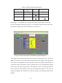
Figure 5.1: Open Loop Evaporator Process menu
73
Figure 5.2: Block Parameter window for feed flow input
73
Figure 5.3: Simulation Parameter window for stop time change
74
Figure 5.4: Output showing the height of tank versus time
74
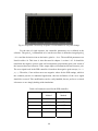
Figure 5.5: Part of Output showing the height of tank versus time
75
Figure 5.6: Output showing the change in concentration with time
77
Figure 5.7: Level Properties window for saving data to a workspace
79
Figure 5.8: Output showing the height of tank versus time
80
Figure 5.9: Polyethylene Process Menu
83
Figure 5.10: Process Flow Diagram of the Polyethylene system
84
Figure 5.11: Block Parameter for hydrogen flow, FH moles/s
84
Figure 5.12: Simulation Results of the Open Loop Polyethylene Reactor
85
Figure 6.1: Process flow sheet of closed-loop evaporator process
89
Figure 6.2: Block Parameter for changing the PID controller settings
90
Figure 6.3: Plot of Concentration with time for a unit step change in P100
90
Figure 6.4: Block Parameter for changing the set point
91
Figure 6.5: Block Parameter for PID controller
91
Figure 6.6: System responses to set point change at gain of –320
93
Figure 6.7: System response to set point change at gain of –350
93
Figure 6.8: Expanded Closed-loop response of concentration to set-point change 93
Figure 6.9: Response of Evaporator Process to set point change using
Cohen-Coon settings
96
Figure 6.10: Response of Evaporator Process to set point change using
Ziegler-Nichols settings
96
Figure 6.11: Effect of Feed Flow disturbance on concentration in open-loop
System
97
Figure 6.12: Effect of feed flow disturbance on concentration in closed-loop
system with Cohen-Coon settings
97
Figure 6.13: Effect of feed flow disturbance on concentration in closed-loop
system with Ziegler-Nichols settings
98
Figure 7.1: Evaporator Process with two control loops
99
vi
Figure 7.2: Open-loop response to disturbance in feed concentration
100
Figure 7.3: Closed-loop response to disturbance in feed concentration
101
Figure 7.4: Closed loop response to disturbance using improved PI settings
101
Figure 7.5: Open loop response for a step change in the steam pressure
104
Figure 8.1: The MSF Process Menu
105
Figure 8.2: Single loop control for MSF process
106
Figure 8.3: Cascade Control Structure for MSF process
107
Figure 8.4: The open loop response for TB0 to step change in Ws
108
Figure 8.5: Product response to disturbance in feed temperature
108
Figure 8.6: Product response to disturbance when single loop is involved
109
Figure 8.7: Product response to disturbance when cascade control is involved
109
Figure 8.8: Feed forward Controller Structure for the Evaporator Process
111
Figure 8.9: FFC structure for Evaporator process showing parameter dialog box
112
Figure 8.10: Process response to step change in the feed concentration
113
vii
Acknowledgment
The investigator would like to thank the general directorate of research center at the
college of engineering for their support, continuous follow up and patience throughout
the project duration. I would like to emphasize the benefit and advantage of this
program, which enables the scientist and scholars to manifest their research ideas into
realistic application.
viii
ABSTRACT
A user manual for the Process Control Laboratory (PCLAB) software is
composed. The PCLAB is a MATLAB-based computer program that simulates certain
chemical processes for dynamic analysis and control. The manual consists of eight
chapters and two appendices. The manual is organized such that the first chapter gives
and overview of the MATLAB basic functions, SIMULINK, and PCLAB. The second
chapter introduces the user to the case studies which comprises of seven common
industrial processes. Brief theoretical background regarding dynamic analysis and
control is discussed in chapter three. Chapter four addresses the steady state disturbance
sensitivity analysis. Chapter five and six cover the open-loop and closed-loop dynamic
analysis, respectively. Chapter seven addresses the control of multivariable systems
while chapter eight investigate advanced topics such as cascade and feed-forward
control configuration.
‫الملخص‬
‫تم اعداد دليل المستخدم لبرنامج مختبر عمليات التحكم )بي سي الب( الذي يعتمد على البرنامج الھندسي ماتالب و‬
.‫ يتكون الكتيب من ثمانية ابواب و ملحقان‬.‫يعنى بمحاكاة العمليات الكيميائيه لدراسة سلوكھا الدينامي و التحكم فيھا‬
‫ و اما الباب الثاني فيستعرض سبع‬.‫يھتم الباب األول يتقديم كل من برنامج ماتالب و سميولنك و بي سي الب‬
‫ و في الباب الثالث يتم تقديم األسس النظريه و‬.‫عمليات تصنيع كيميائيه و التي ستسخدم كاساس للدراسات التجريبيه‬
‫ فيما يخص تحليل حساسية اإلطضرابات في حالة‬.‫المعادالت الرياضيه الخاصه بالتحكم و ديناميكية العمليات‬
‫اإلستقرار فتناقش في الباب الرابع بينما يختص الباب الخامس و السادس بعرض الدروس الخاصه بالتحليل الدينامي‬
‫ كما يخصص الباب السابع لمعالجة عمليات التحكم متعددة المتغيرات و الباب الثامن‬.‫للدائرة المفتوحة و المغلقه‬
.‫لعمليات التحكم المتقدمه مثل الدوائر المركبه و التغذيه األماميه‬
ix
CHAPTER 1: INTRODUCTION
1.1 OBJECTIVES
The PCLAB software is developed based on MATLAB tools and functions
including SIMULINK (a graphical simulation Toolbox). Therefore, the aim of this
chapter is to introduce the student to MATLAB and SIMULINK as well as explain the
basic operations and installation of the PCLAB software. A brief description of
MATLAB and SIMULINK will be presented, further information can be found in
printed document or online documents provided by MATLAB Inc.
1.2 WHAT IS MATLAB
MATLAB is developed by Math Works Inc. It contains over 200 mathematical
subprograms that enables the engineer to solve a broad range of mathematical problems
including complex arithmetic, eigen-value problems, differential equations, linear and
non-linear systems and many other special functions.
MATLAB is a powerful tool that is widely applied to solve many problems in
process control and dynamics. In order to be able to fully apply PCLAB, one must be
familiar with MATLAB commands. A few examples of the MATLAB commands are
given below to familiarize the user with the software and as one practices, he becomes
exposed to more and more commands.
When the software is loaded to the computer memory, the prompt ‘>>’ is
displayed. The program is in an interactive command mode. If an expression is entered
with the correct syntax, it is processed immediately and the result displayed on the
screen. The tutorials below are intended to introduce the reader to MATLAB so as to
give the students handy experience with the features that are essential to understanding
and evaluation of the software.
1.3 BASIC OPERATIONS AND COMMANDS
The four elementary arithmetic operations in MATLAB are done by the
operators +, -, *, /, and ^, where, ^ , stands for power operator: For example, type the
following and then press ‘Enter’ key and observe the result.
1
»2+3*4^(1-1/5)
The operator \ is for left division. For example, try:
»2/4
»2\4
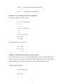
Example 1. Using MATLAB as a calculator
At the prompt type 4321+8765
>>4321+8765 (hit enter)
Ans = 13086
Or try to solve the expression 2*3+4/5*1.5+11
>>2*3+4/5*1.5+11 (hit enter)
ans = 18.2
MATLAB easily handles complex and infinite numbers:
»sqrt( -1)
Ans = 0 + 1.0000i
Both i and j stand for the complex number (that is square root of –1) unless another
value is assigned to them. Also the variable pi represents the ratio of the circumference
of a circle to its diameter (i.e., 3.141592653.. .). If an expression cannot be evaluated,
MATLAB returns NaN, which stands for Not-a-Number:
The equality sign is used to assign values to variables:
»a = 2
»b = 3*a
If no name is introduced, result of the expression is saved in a variable named ans:
»a+b
If you do not want to see the result of the command, put a semicolon at the end of it:
»a+b;
2
You can see the value of the variable by simply typing it:
»a
MATLAB is case sensitive. This means MATLAB distinguishes between upper
and lower case variables. In MATLAB all computations are done in double precision.
However, the result of calculation is normally shown with only 5 digits. The format
command may be used to switch between different output display formats:
»c = exp(pi)
»format long, c
»format short e, c
»format long e, c
»format short, c
The clc command clears the command window and homes the cursor:
»clc
Remember that by using the up arrow key you can see the commands you have entered
so far in each session. If you need to call a certain command that has been used already,
just type its first letter (or first letters) and then use the up arrow key to call that
command.
Several navigational commands from DOS and UNIX may be executed from the
MATLAB Command Window, such as cd, dir, mkdir, pwd, Is. For example:
»cd d:\matlab\toolbox
»cd 'c:\Program Files\Numerical Methods\Chapterl '
The single quotation mark (') is needed in the last command because of the presence of
blank spaces in the name of the directory.
3
1.3.1 Vectors and Matrices
MATLAB is designed to make operations on matrices as easy as possible. Most
of the variables in MATLAB are considered as matrices. A scalar number is a l x l
matrix and a vector is a 1 x n (or n x 1) matrix. Introducing a matrix is also done by an
equality sign:
»m = [1 2 3; 4, 5, 6]
Note that elements of a row may be separated either by a space or a comma, and the
rows may be separated by a semicolon or carriage return (i.e., a new line). Elements of a
matrix can be called or replaced individually:
»m(1,3)
»m(2,1) = 7
Matrices may combine together to form new matrices:
»n = [m; m]
»o = [n, n]
The transpose of a matrix results from interchanging its rows and columns. This can be
done by putting a single quote after a matrix:
»m = [m; 7, 8, 9]'
A very useful syntax in MATLAB is the colon operator that produces a row vector:
»v = -1:4
The default increment is 1, but the user can change it if required:
»w = [-1:0.5:4; 8:-1:-2; 1:11]
A very common use of the colon notation is to refer to rows, columns, or a part of the
matrix:
»w(:,5)
»w(1,:)
»w(2:3,4:7)
4
»w(2,8:end)
Two useful array functions are size, which gives the size of the array, and length, which
gives the maximum length of the array:
»size(w)
»length(w)
1.3.2 Array Arithmetic
Multiplying a scalar to an array, multiplies all the elements by the scalar:
»a = [1, 2, 4; 2:4; 4:0.5:5], 2*a
Only two arrays of the same size may be added or subtracted:
»b = ones(3); a-b
»c = ones(3,1); a-c
Adding a scalar to an array results in adding the scalar to all the elements of the array:
»a+2
Vector and matrix multiplication requires that the sizes match:
»a*b
»c'*a
To perform an operation on an array element-by-element, use a "." before the operator:
»a.*b
»a^2
»a.^2
» l./a
Some useful matrix functions are:
»det(a)
determinant of a square matrix
»inv(a)
inverse of matrix
»rank(a)
rank of matrix
»eig(a)
eigenvalues and eigenvectors of square matrix
5
»poly(a)
characteristic polynomial of matrix
»svd(a)
singular value decomposition
Example 2. Using MATLAB for matrix calculations
Enter the example below at the prompt
>> b = [1 2;3 4] (hit enter)
b= 1 2
3 4
c = [5 6; 7 8] ( hit enter)
c= 5 6
7 8
>> d = b*c (hit enter)
ans = 19 22
43 50
To find the transpose of d, type d’
>> d’ (enter)
ans = 19 43
22 50
Example 3 Using MATLAB elementary math functions
The software also has several elementary math functions. These include trigonometric
functions, exponential functions and other built-in matrix functions like determinant,
rank and null-space. Examples of trigonometric and exponential functions are:
Trigonometric functions
>> cos(2) (hit enter)
ans= -0.4161
6
>>sin(pi) (hit enter)
ans = 1.2246e-16
Exponential functions
>>exp(1)
(hit enter)
ans = 2.7183
>>log(2)
(hit enter)
ans = 0.6931
1.3.3 Graphics
The program also has outstanding graphic capabilities. It can be done with automatic
scaling or within defined scales as shown in the example below
>> x = -10: .1 :10;
>>plot ( x.^2 )
>>figure
>>plot (x, x.^2 )
>>figure
1.3.3.1 Plotting graphs
2-D Graphs: Functions with one independent variable can easily be visualized in
MATLAB:
»x = linspace(0,2); y = x.*exp(-x);
»plot(y)
plots y versus their index
»plot(x,y)
plots y against x
»grid
adds grid lines to the current axes
»grid
removes the grid lines
»xlabel('x')
adds text below the x-axis
»ylabel('y')
adds text besides the y-axis
»title('y = x*exp( -x)')
adds text at the top of the graph
»gtext('anywhere')
places text with mouse
7
»text(1,0.2,’(1,0.2)’)
places text at the specific point
You can use symbols instead of lines. You can also plot more than one function in a
graph:
»plot(x,y,'.' ,x, x.*sin(x))
Also, more than one graph can be shown in different frames:
»subplot(2,1,1), plot(x,x.*cos(x))
»subplot(2,1,2), plot(x,x.*sin(x))
Axis limits can be seen and modified using the axis command:
»axis
»axis([0, 1.5,0, 1.5])
Before continuing, clear the graphic window:
»clf
Another easy way to plot a function is:
»fplot('x*exp(-x)',[0,2])
The function to be plotted may also be a user-defined function.
1.3.4 Scripts and Functions
The programs written in the language of MATLAB should be saved with the
extension of "m", from where the name of m-file comes. When using the editor of
MATLAB, it automatically saves your files with the "m" extension. Otherwise, one
should be sure to save them with the "m" extension. M-files can be in the form of
scripts and functions and could be executed in the MATLAB workspace.
A script is simply a series of MATLAB commands that could have been entered
in the workspace. When typing the name of the script, the commands will be executed
in their sequential order as if they were individually typed in the workspace. For
example, let us calculate the volume of an ideal gas as a function of pressure and
temperature. Type the following commands in the editor and save it as "myscript.m":
8
% A sample script file
disp(' Calculating the volume of an ideal gas.')
R = 8314;
% Gas constant
t = input(' Vector of temperatures (K) = ');
p = input(' Pressure (bar) = ')*le5;
v = R *t/p;
% Ideal gas law
% Plotting the results plot(t,v)
xlabel('T (K)')
ylabel('V (m^3/kmol)')
title('Ideal gas volume vs temperature')
The symbol % indicates that this line contains comments. The % sign, and what comes
after it in that line, will be ignored at the time of execution. Return to the MATLAB
command window and type:
»myscript
Input the required data and see the results.
1.3.5 Flow Control
MATLAB has several flow control structures that allow the program to make
decisions or control its execution sequence. These structures are for, if, while, and
switch which we describe briefly below:
If….(else…) end -The if command enables the program to make decision about what
commands to execute:
x=input(' x= ');
if x >= 0
y = x^2
end
9
You can also define an else clause, which is executed if the condition in the if statement
is not true:
x = input(' x = ');
if x>=0
y = x^2
else
y = -x^2
end
for….end –The for command allows the script to cause a command, or a series of
commands, to be executed several times:
k=0;
for x = 0:0.2:1
k=k+l
y(k) = exp( -x)
end
while…end -The while statement causes the program to execute a group of commands
until some condition is no longer true:
x=0;
while x<l
y= sin(x)
x = x+0.1;
end
switch…case….end -When a variable may have several values and the program has to
execute different commands based on different values of the variable, a switch-case
structure is easier to use than a nested if structure:
a = input('a = '); switch a case 1
disp('One'); case 2
disp('Two')
10
case 3
disp('Three')
end
Two useful commands in programming are break and pause. You can use the break
command to jump out of a loop before it is completed. The pause command will cause
the program to wait for a key to be pressed before continuing:
k=0;
for x = 0:0.2:1
if k>3
break
end
k = k+l
y(k) = exp( -x)
pause
end
1.3.6 Data Export and Import
There are different ways you can save your data in MATLAB. Let us first
generate some data:
»a = magic(3); b = magic(4);
The following command saves all the variables in the MATLAB workspace in the file
"f1.mat':
»save f1
If you need to save just some of the variables, list their names after the file name. The
following saves only a in the file "f2.mat":
»save f2 a
The files generated above have the extension ".mat" and could be retrieved only by
MATLAB.
11
To use your data elsewhere you may want to save your data as text:
»save f3 b -ascii
Here, the file "f 3" is a text file with no extension.
You can load your data into the MATLAB workspace using the Load command. If the
file to be loaded is generated by MATLAB (carrying ".mat" extension), the variables
will appear in the workspace with their name at the time they were saved:
»clear
»load fl
12
1.4 INTRODUCTION TO SIMULINK
SIMULINK is an interactive programming environment within MATLAB
which provides graphical interface to MATLAB programs. The program is user-friendly
and one can run simulations of linear and nonlinear systems interactively. The system
can then be analyzed and the results easily visualized by simple click-and-drag of
mouse operations.
Although the standard MATLAB package is useful for analysis of linear
systems, SIMULINK is far more useful for the simulation of control system. It enables
the rapid construction and simulation of control block diagrams. In order to make it easy
for learning SIMULINK, the reader is taken through different tutorials. The goal of the
tutorial is to introduce the use of SIMULINK for control system simulation. The
tutorials are divided into sections namely; Background, Open-loop Simulations, Closedloop Simulations
1.4.1 Background
The first step is to startup MATLAB on the machine you are using. In the Launch
Pad window of the MATLAB desktop, select SIMULINK and then the SIMULINK
Library Browser. This is done through the steps below:
1. In your PC, double click the MATLAB icon. As a result, a MATLAB command
window pops up and becomes ready for operation.
2. Change the operating directory to the subdirectory under which a specific
tutorial exist by typing, At the MATLAB command prompt, the following:
>> cd C:\workshop\simulink\MPC
(This will put you in the subdirectory designated for Model predictive
simulations)
Or
>> cd C:\workshop\simulink\ident
13
(This will put you in the subdirectory designated for identification simulations)
Or
>> cd C:\workshop\simulink\phlink
(This will put you in the subdirectory designated for pH process simulations)
etc…
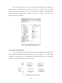
While in the SIMULINK Library Browser number of options are listed, as shown in
Figure 1.1. Notice in this figure that Continuous has been highlighted; this will provide a
list of continuous function blocks available. Selecting Continuous will provide the list
of blocks shown in Figure 1.2. The ones that we often use are Transfer Fcn and StateSpace.
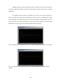
Fig. 1.1 SIMULINK Library Browser
14
Fig. 1.2 SIMULINK Continuous Blocks.
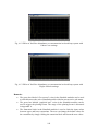
Selecting the Sources icon yields the library shown in Fig. 1.3. The most
commonly used sources are Clock (which is used to generate a time vector), and Step
(which generates a step input).
Fig. 1.3 SIMULINK Sources Library
15
The Sinks icon from Fig. 1.1 can be selected to reveal the set of sinks icons
shown in Fig. 1.4. The one that we use most often is the To Workspace icon. A variable
passed to this icon is written to a vector in the MATLAB workspace. The default data
method should be changed from “structure” to “matrix” in order to save data in an
appropriate form for plotting.
Fig. 1.4 SIMULINK Sinks Library.
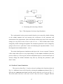
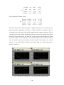
1.4.2 Open-Loop Simulation
A user now has enough information to generate an open-loop simulation. The
Clock, simout, step and Transfer function blocks can be dragged to a model (.mdl)
workspace, as shown in Fig. 1.5a. Renaming the blocks and variables, and connecting
the blocks, produces the model shown in Fig. 1.5b.
a. Placement of function blocks
16
b. Renaming and connecting of blocks
Fig. 1.5 Development of an Open-loop Simulation
The s-polynomials in the process transfer function were entered by double-clicking
on the transfer function icon and entering the coefficients for the numerator and
denominator of the polynomials. Notice also that the default step (used for the step input
change) is to step from a value of 0 to a value of 1 at t = 1. These default values can be
changed by double-clicking the step icon. The simulation parameters can be changed by
going to the Simulation “pull-down” menu and modifying the stop time (default = 10) or
the integration solver method (default = ode45).
The reader should generate simulations and observe the “inverse response” behavior
of the output with respect to a step input change. Use the subplot command to place the
process output (y) on the top plot, and the manipulated input (u) on the bottom plot. If
desired, change the default simulation stop time by selecting the parameters “pull
down” menu.
1.4.3 Feedback Control Simulation
The Math icon from Fig. 1.2 can be selected, resulting in the functions shown in
Fig. 1.6. Additional icons can be found by selecting the Simulink Extras icon in Fig. 1.1.
Selecting the Additional Linear icon from this group yields the set of icons in Fig. 1.7.
The most useful icon here is the PID Controller. Any icon can be “dragged” into the
17
untitled model workspace. In Fig. 1.8 we show the preliminary stage of the construction
of a control block diagram, where icons have been dragged from their respective
libraries into the untitled model workspace.
Fig. 1.6 SIMULINK Math Library.
Fig. 1.7 SIMULINK Additional Linear Library.
18
The labels (names below each icon) can easily be changed. The default
parameters for each icon are changed by double clicking the icon and entering new
parameter values. Also, connections can be made between the outputs of one icon and
inputs of another. Fig. 1.8b shows how the icons from Fig. 1.8a have been changed and
linked together to form a feedback control block diagram.
It should be noted that the form of the PID control law used by the SIMULINK
PID Controller icon is not the typical form that we use as process control engineers. The
form can be found by double-clicking the icon to reveal the following controller transfer
function representation while we normally deal with the following PID structure P = kc,
I = kcI, D = kcD.
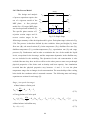
Fig. 1.8. Block Diagram for Feedback Control of the Van de Vusse CSTR
The s-polynomials in the process transfer function were entered by doubleclicking on the transfer function and entering the coefficients for the numerator and
denominator polynomials.
Notice also that the default step (used for the step set-point change) is to step
from a value of 0 to a value of 1 at t = 1. These default values can be changed by
double-clicking the step icon. The simulation parameters can be changed by going to
the Simulation “pull-down” menu and modifying the stop time (default = 10) or the
integration solver method (default = ode45).
19
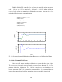
Double click the PID controller box and enter the controller tuning parameters
of kc = 1.89 and τI = 1.23 by entering P = 1.89 and I = 1.89/1.23 in the default PID
Controller block and run the simulation by clicking the start button. Generate Fig. 1.9 by
typing the following on the command window.
» subplot(2,1,1),plot(t,r,'--',t,y)
» xlabel('t (min)')
» ylabel('y (mol/l)')
» subplot(2,1,2),plot(t,u)
» xlabel('t (min)')
» ylabel('u (min^-1)')
1.5
y (mole/l)
1
0.5
0
-0.5
0
1
2
3
4
5
t (min)
6
7
8
9
10
0
1
2
3
4
5
t (min)
6
7
8
9
10
u (1/min)
3
2
1
0
Fig. 1.9. Measured Output & Manipulated Input Responses to a Unit Set point Change.
1.4.4 Other Commonly Used Icons
Often you will want to simulate the behavior of systems that have time delays.
The Transport Delay icon can be selected from the Continuous library shown in Fig. 1.2. The
transport delay icon is shown in Fig. 1.10. Our experience is that simulations can
become somewhat “flaky” if 0 is entered for a transport delay. We recommend that you
remove the transport delay block for simulations where no time-delay is involved.
20
Fig. 1.10 Transport Delay Icon
Manipulated variables are often constrained to between minimum (0 flow, for example)
and maximum (fully open valve) values. A saturation icon from the Nonlinear library can
be used to simulate this behavior. The saturation icon is shown in Fig. 1.11.
Fig. 1.11. Saturation Element
Actuators (valves) and sensors (measurement devices) often have additional dynamic
lags that can be simulated by transfer functions. These can be placed on the block
diagram in the same fashion that a transfer function was used to represent the process
earlier.
It should be noted that icons can be “flipped” or “rotated” by selecting the icon
and going to the format “pull-down” menu and selecting Flip Block or Rotate Block. The
block diagram of Fig. 1.8 has been extended to include the saturation element and
transport delay, as shown in Fig. 1.12.
Fig. 1.12. Block Diagram with Saturation and Time-Delay Elements
21
The default data method for the “to workspace” blocks (r,t,u,y in Fig. 1.12) must be
changed from “structure” to “matrix” in order to save data in an appropriate form for
plotting.
In conclusion, SIMULINK is a very powerful block diagram simulation
language. Simple simulations, including the majority of those used as examples in this
textbook, can be set-up rapidly (in a matter of minutes). The goal of this module was to
provide enough of an introduction to get you started on the development of open- and
closed-loop simulations. With experience, the development of these simulations will
become second-nature. It is recommended that you perform the simulations shown in
this module, as well as other exercises, to rapidly acquire these simulation skills.
1.5 INSTALLING PCLAB
For better performance, simply copy the PCLAB folder into your local hard
disk. Then either add this directory to your MATLAB path using the path command or
choose to work from the designated directory for PCLAB using the cd command. Note
that the working directory can be adjusted directly from the menu of the MATLAB
Command Window. PCLAB works for MATLAB version 5.3 and higher.
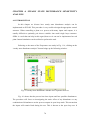
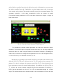
Fig. 1.13 Main menu of the PCLAB software
22
To start PCLAB, first lunch your MATLAB. Once in the MATLAB program,
use the path browser to change to PCLAB subdirectory. Then type mainmenu at the
MATLAB command prompt, this will take you to the itemized menu of PCLAB from
which you can select the case study you want to work on. Fig. 1.13 shows the main
menu of PCLAB.
1.6 OVERVIEW OF PCLAB STRUCTURE
PCLAB is interactive simulation software for process control analysis and
training. The process control module contains several exercises that cover basic concept
of process dynamic and control. These exercises can be carried out on simulated
processes that are very common in the chemical engineering industry such as distillation
columns, reactors and evaporators. The exercises are unified for all case studies. This
means that the user can choose a relevant case study and work on the pre-designed
exercises. PCLAB is based on menu structure that allows the user to navigate through
various case studies each of which has its own submenu that comprises the designated
exercises. By practicing on these tutorials, the user then learns different aspects of
dynamic analysis and control design.
The structure of the software is designed in a user–friendly, menu-driven
framework such that the process engineer can easily navigate through the various parts
of the program, carry out simulation experiments, visualize the results and draw
conclusions on the effect of different design parameters, and control configurations.
There is a Main menu (Fig. 1.13) that allows the user to choose from different
case studies. The case studies covered by the current version of PCLAB are as follows:
1. Forced-Circulation Evaporator
2. Polyethylene Reactor
3. Fluid catalytic Cracking Unit
4. Ethylene Dimerization Process
5. Double Effect Evaporator
6. Two-CSTR in Series
7. Multi-Stage Flash Desalination Plant
23
These basic case studies represents the heart of the chemical engineering industry
can be used in combination with the exercises to generate a whole lot of scenarios that
will enhance the understanding of the basics of control process analyses.
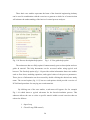
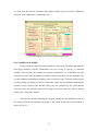
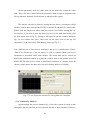
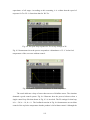
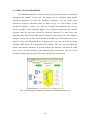
Fig. 1.14 Process description help option
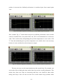
Fig. 1.15 User guide help option
The main menu has two Help option’s buttons namely process description and user
guide & tutorial. The help documents can be accessed online using typical web
browser. The first help option (fig. 1.14) provides online information about case studies
such as flow sheet, modeling equations, and typical values of the process parameters.
These pieces of information can be accessed by double clicking the desired case study
name. The second option (fig. 1.15) has two sub-options which provide overview of
PCLAB and procedure for carrying out certain tutorials.
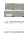
By clicking one of the case studies, a sub menu will appear. See for example
Fig. 1.16 which shows a typical sub-menu for the forced-circulation process. This
submenu allows the user to select a specific tutorial within several exercises that are
ordered as follows:
1. Open-Loop
2. Closed-Loop (PID control)
24
3. Multi-Loop (PID control)
4. Feed Forward Control
5. Steady State Disturbance Analysis
6. System Identification.
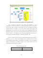
Fig. 1.16 Evaporator menu
The aforementioned exercise focuses on the following objectives:
•
Modeling of the process
•
Controller design and tuning
•
Sensitivity analysis and system identification
The Tutorial is organized in such a way as to lead the user to the proper
understanding of process dynamics. First the process is developed for steady state
predictions. Since chemical process systems do not reach steady state instantaneously,
accurate modeling must capture both the steady state and transient behavior of the
system. The transient behavior is the time-dependent trajectory of an output in response
to a particular input or class of inputs. After that control synthesis is the nest step,
where the control structures are selected and tuned. Finally the designed controlled
system is analyzed for proper performance. Future versions of the software can examine
advance control algorithms such as Internal Model Control (IMC) as well as Model
Predictive Control (MPC).
25
The sub menu in Fig. 1.16 has additional navigation buttons. The “process
description” button allows the user to access a document file containing the description
of the current active (selected) case study. The yellow button simply closes the current
submenu and returns the user to the main menu.
PCLAB also includes additional features which will be discussed as we progress
in the manual.
26
CHAPTER 2: CASE STUDIES
2.1 INTRODUCTION
In this chapter, the modeling of the basic case studies (representing the heart of
the chemical engineering industry) is undertaken. Tutorials and exercises that can be
carried out upon these case studies will be discussed in other chapters. These modules
(case studies) are clearly defined and all involved parameters are explained. It is
important to understand the mathematical development of the models as they represent
the basis to which the exercises will be referred to. The mathematical models developed
here for each case study are core to the process transfer functions that will be used with
differing controller algorithms and are classical examples from literature.
As listed earlier, these case studies are;
8. Forced-Circulation Evaporator
9. Polyethylene Reactor
10. Waste Water Treatment Unit
11. Ethylene Dimerization Process
12. Double Effect Evaporator
13. Two-CSTR in Series
14. Multi-Stage Flash Desalination Plant
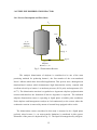
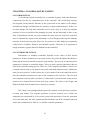
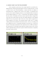
2.2 FORCED-CIRCULATION EVAPORTOR UNIT
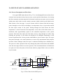
2.2.1 Process Description and Flow sheet
The forced-circulation evaporator is a common processing unit in sugar mills,
alumina production and paper manufacture. This process is used to concentrate a dilute
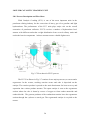
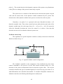
liquor by evaporating its solvent (usually water) as shown in the Fig. 2.1.
A feed stream with solute of concentration C1 (mass percentage) is mixed with
high volumetric recycle flow rate and fed to a vertical evaporator (heat exchanger). The
solution will pass through the tube. A saturated steam is used to heat up the mixture by
condensing on the outer surface of the tubes. The liquor which passes up inside the tube
27
boils and then passes to a separator vessel. In the separator, the liquid and vapor are
separated at constant temperature and pressure. The liquid is recycled with some being
drawn off as product with solute concentration of C2. The vapor is usually condensed
with water. Water is used as the coolant.
F4
Separator
Cooling
water
F200 T200
Steam
L2
F5
P 100 F100 T100
P2
F3
Product
Feed
F1 C1 T1
F2 C2 T2
Fig. 2.1 Flow sheet of Forced Circulation Evaporator Process
2.2.2 The Process Model
ρA
dL2
= F1 − F4 − F2
dt
M
dC 2
= F1C1 − F2 C 2
dt
W
(2.1)
(2.2)
(2.3)
dP2
= F4 − F5
dt
Additional relations:
28
(2.4)
T2 = 0.5616P2 + 0.3126C 2 + 48.43
T3 = 0.507 P2 + 55.0
(2.5)
F2 = F1 − F4
(2.6)
F4 = [Q100 − F1Cp (T2 − T1 )] / λ
(2.7)
T100 = 0.1538P100 + 90.0
(2.8)
Q100 = F100 λs = UA1 (T100 − T2 )
(2.9)
Q200 = F200 Cp (T201 − T200 ) = UA2 (T3 − 0.5 * (T200 + T201 ))
(2.10)
F5 = Q200 λ
(2.11)
UA1 = 0.16( F1 + F3 )
(2.12)
2.2.3 Process Parameters and Variables
Variable
Description
Value
Units
F1
Feed flow rate
10.0
kg/min
F2
Product flow rate
2.0
kg/min
F3
Circulating flow rate
50.0
kg/min
F4
Vapor flow rate
8.0
kg/min
F5
Condensate flow rate
8.0
kg/min
C1
Feed composition
5.0
Percent
C2
Product composition
25.0
Percent
T1
Feed temperature
40.0
C
T2
Product temperature
84.6
C
29
T3
Vapor temperature
80.6
C
L2
Separator level
1.0
m
P2
Operating pressure
50.5
kPa
F100
Steam flow rate
9.3
kg/min
T100
Steam temperature
119.9
C
P100
Steam pressure
194.7
kPa
Q100
Heater duty
339.0
kW
F200
Cooling water flow rate
208.0
Kg/min
T200
Cooling water inlet temperature
25.0
C
T201
Cooling water outlet temperature
46.1
C
Q200
Condenser duty
307.9
kW
ρA
Mass holdup in the separator
20
kg/m
M
Solute holdup
20
kg
W
Constant
4
kg/kPa
λ
Latent heat of vaporization of water
38.5
kW/kg
UA2
Heat transfer coefficient times the heat 6.84
kW/K
transfer area
λs is the latent heat of steam which is calculated from a given correlation as a function
of the saturation temperature.
30
2.3 ETHYLENE POLYMERIZATION REACTOR
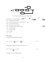
2.3.1 Process Description and Flow sheet
Polyethylene is considered the world largest produced synthetic commodity polymer.
The polyethylene reactor process
P M1, P M2, P H2, P N2
is depicted in Fig. 2.2. The
Bt
process model was developed by
McAuley et al. [12] and is given
below.
Fg
The major components of the
process are: (a) feed gas which is
partly
Fc
combined
with
the
recycled gas before entering the
bubbling fluidized bed, the other
part of the fresh feed gas is used
to introduce the Ziegler-Natta
Op
Tgi
a product withdrawal system
Tg
which is controlled in order to
FM1, FM2, FH2, FN2
Fw, Twi
Two
catalyst; (b) a catalyst feeder; (c)
maintain a constant bed height
Tf
inside
the
recycling
Fig. 2.2 Polymerization Reactor
reactor;
which
(d)
includes
gas
a
cyclone and a compressor; (e) reactor with catalyst disengagement zone. Four major
components are fed to the reactor. The gaseous species are Ethylene (monomer), Butene
(comonomer), hydrogen and nitrogen. The nitrogen is used to carry the catalyst powder
and maintain the desired column pressure. In this process, the bed temperature is
controlled by manipulating the feed temperature of the cooling water. The total pressure
is controlled by manipulating the bleed flow. And the bed height is regulated by the
discharge system. The discharge system operates periodically, i.e. the outlet flow valve
opens every time the bed level exceeds certain limit.
31
2.3.2 The Process Model
Vg
dC M 1
= FM 1 − x M 1 Bt − RM 1
dt
(2.13)
Vg
dC M 2
= FM 2 − x M 2 Bt − RM 2
dt
(2.14)
Vg
dC H
= FH − x H Bt − R H
dt
(2.15)
Vg
dC N
= FN − x N Bt
dt
(2.16)
dYc
= Fc ac − k d Yc − O pYc / Bw
dt
( M r Cp r + BwCp p )
M g Cp g
dTg
dt
(2.17)
dT
= HF + HG − HR − HT − HP
dt
= Fg Cp g (Tgi − Tg ) + Fw Cp w (Twi − Two )
Pt = (C M 1 + C M 2 + C H + C N ) RT
Tgi = (
(2.18)
(2.19)
(2.20)
Pt
) (1−η) / η T
Pt + ΔP
(2.21)
FwCp w (Twi − Two ) = 0.5UA[(Two + Twi ) − (Tgi + Tg )]
(2.22)
HF = ( FM 1Cp M 1 + FM 2 Cp M 2 + FH Cp H + FN Cp N )(T f − Tref )
(2.23)
HG = Fg Cp g (Tg − Tref )
(2.24)
HT = ( Fg + Bt )Cp g (T − Tref )
(2.25)
HP = O p Cp p (T − Tref )
(2.26)
HR = M w1 RM 1ΔH r
(2.27)
O p = M w1 RM 1 + M w 2 RM 2
(2.28)
RM 1 = C M 1Yc k p1e
E
− (1 / T −1 / Tref )
R
RM 2 = C M 2Yc k p 2 e
(2.29)
E
− (1 / T −1 / Tref )
R
(2.30)
32
Cp g = ∑ xi Cpi
(2.31)
2.3.3 Process Parameters and Variables
Variable
Description
Value
Units
ac
Active site concentration
0.548
mole/kg
Bw
Mass of the polymer in the bed
70.0
tonne
Bt
Bleed flow rate
10.39
mole/s
CM1
Concentration of monomer,
297.06
mole/m3
CM2
Concentration of co-monomer
116.17
mole/m3
CN
Concentration nitrogen
166.23
mole/m3
CH
Concentration of hydrogen
105.78
mole/m3
CpM1
Heat capacity of monomer
11
cal/mole K
CpM2
Heat capacity of co-monomer
24
cal/mole K
CpH
Heat capacity of hydrogen
7.7
cal/mole K
CpN
Heat capacity of nitrogen,
6.9
cal/mole K
Cpw
Heat capacity of recycle gas and water
18.0
cal/mole K
Cpp
Heat capacity of polymer,
0.85
cal/g K
E
Activation energy for propagation,
9000
cal/mole
Fc
Catalyst flow rate
2.0
kg/s
Fw
Cooling water flow rate,
5.6x105
mole/s
Fg
recycle flow rate,
8500
mole/s
FM1
Monomer flow rate,
131.13
mole/s
FM2
co-monomer flow rate,
3.51
mole/s
FN
hydrogen flow rate,
1.6
mole/s
FH
nitrogen flow rate,
2.52
mole/s
kd
Deactivation rate constant,
0.0
1/s
kp 1
Propagation rate constant for monomer
85.0
L/mole s
kp 2
Propagation rate constant for co-monomer,
3.0
L/mole s
Mw
Water holdup in the heat exchanger,
2x106
mole
MrCpr
Thermal capacitance of the reaction vessel,
14x106
kcal/K
Op
Polymer outlet rate,
3.6434
kg/s
Pt
Total pressure,
20.0
atm
PM1
Partial pressure of monomer
8.67
atm
33
PM2
Partial pressure of co-monomer
3.39
atm
PN
Partial pressure of nitrogen
4.8525
atm
PH
Partial pressure of hydrogen,
3.0875
R
atm
-6
Ideal Gas constant,
82.6x10
atm
mole
T
Bed temperature,
82
o
C
Tf
feed temperature,
25
o
C
Tref
reference temperature,
87
o
C
Tgi
Temperature of recycle stream before cooling
136
o
C
C
Tg
Temperature of recycle stream after cooling,
51.7
o
Twi
Cooling water temperature before cooling,
20
o
C
Two
Cooling water temperature after cooling,
35
o
C
Yc
Number of moles of catalyst site, mole
5.849
mole
ΔHr
Heat of reaction
-894
cal/g
The system has two internal (built-in) PI control loops which are set as:
Control loop
kc
τI
Pt Æ Bt
10
10
T Æ Tw
3
20
34
m3/K
2.4 ETHYLENE DIMERIZATION REACTOR
2.4.1 Process Description and Flow Sheet
TR
W, Tc
F, Tf
Ethylene
Catalyst
W, Tco
(1-β)Q, T
Q, T
Ethylene
Butene, C6, C8
\
βQ, T
Fig. 2.3 Dimerization Reactor
The catalytic dimerization of ethylene is considered to be one of the most
promising methods for producing butene-1, the first member of the even-numbered
linear 1-alkenes which have diversified applications. This process uses a homogeneous
titanium-based catalyst which demonstrates high dimerization activity coupled with
excellent selectivity to butene-1 at moderate pressure (20-30 psia) and temperature (5060 oC). The dimerization reaction is regarded as a degenerate ethylene polymerization
reaction and therefore the formation of heavier oligomers is expected. The industrial
ethylene diemrization reactor is operating in liquid phase at bubble point conditions.
Fresh ethylene and homogenous catalyst are fed continuously to the reactor where the
exothermic reaction is removed by means of external loop equipped with a cooler.
The dimerization reactor considered in this study is assumed to be a liquid phase
perfectly mixed reactor, i.e. no mass transfer limitation is considered in this system.
Schematic of the process is depicted in Fig. 2.3. The liquid is homogenized by a high re35
circulation rate around the reactor through a heat exchange used to remove the high
exothermic heat of reaction. The model uses the Homo- and Co-polymerization
mechanisms suggested by Galtier et. al. [9]. The reaction stages; initiation, propagation
and termination are of first order kinetics with respect to each reactant.
Initiation and propagation stages:
K + C 2 n → KC 2 n ,
n ≥1
KC 2 m + C 2 n → KC 2 ( n + m )
n, m ≥ 1
(2.32)
(2.33)
The rate of initiation and propagation, which also represent the rate of disappearance of
C2n in these stages, have the following rate equation:
∞
ra2 n = a 2 n [C 2 n ]∑ [ KC 2 m ]
(2.34)
m=0
Termination stage:
KC 2 m + C 2 n → K + C 2 ( n + m ) , n, m ≥ 1
(2.35)
The chain termination reactions, which are assumed to occur in parallel with the growth
reactions have the following rate equations:
∞
rb2 n = b2 n [C 2 n ]∑ [ KC 2 m ]
(2.36)
m =1
The rate constants are defined as follows:
a2 = a20 e
1 1
− E1 ( − )
T Tr
36
(2.37)
a4 = a40 e
b4 = a 40 e
1 1
− E1 ( − )
T Tr
(2.38)
1 1
− E1 ( − )
T Tr
(2.39)
b2 = b20 a2 e
(2.40)
1 1
− E2 ( − )
T Tr
Based on the above assumptions and the assumed reaction kinetics, the resulted
dynamic model of the dimerization process is presented in the following [1],[6].
2.4.2 The Process Model
V
dC4
= −QβC4 − V [(−b2C2 + a4C4 + b4C4 ) K 2 + a4C4 K + b4C4 K 4 ]
dt
(2.41)
V
dC 2
= FC 2 f − QβC 2 − V [a 2 C 2 ( K + K 2 + K 4 ) + b2 C 2 ( K 2 + K 4 + K 6 )]
dt
(2.42)
V
dC6
= − FC6 + V [b4C4 K 2 + b2C2 K 4 ]
dt
(2.43)
V
dC8
= − FC8 + V [b4C 4 K 4 + b2C2 K 6 ]
dt
(2.44)
V
dK
= FK f − QβK − V [(a 2 C 2 + a 4 C 4 ) K + b2 C 2 ( K 2 + K 4 + K 6 ) + b4 C 4 ( K 2 + K 4 )]
dt
(2.45)
VρC p
dT
= Fρ f C pf (T f − Tr ) + Q (1 − β ) ρC p (TR − Tr ) − QρC p (T − Tr ) + V (r2 (−ΔH1 ) + r4 (−ΔH 2 ))
dt
Vc ρC p
dTR
= Q (1 − β ) ρC p (T − TR ) − UA(TRav − Tcav )
dt
(2.46)
(2.47)
V
dK 2
= −QβK 2 + V [a 2 C 2 K − (a 2 C 2 + a 4 C 4 + b2 C 2 + b4 C 4 ) K 2 ]
dt
(2.48)
V
dK 4
= −QβK 4 + V [a 2 C 2 K 2 − (a 2 C 2 + b2 C 2 + b4 C 4 ) K 4 + a 4 C 4 K ]
dt
(2.49)
V
dK 6
= −Qβ K 6 + V [a 2 C 2 K 4 − b2 C 2 K 6 + a 4 C 4 K 2 )]
dt
(2.50)
where
37
T + TR
2
(2.51)
Tc + Tco
2
(2.52)
TRav =
Tcav =
The dynamic of the outlet temperature of the coolant fluid is not included and
alternatively it is obtained by solving the steady-state equation:
(2.53)
WCp w (Tco − Tc ) = U h Ac (TRav − Tcav )
2.4.3 Process Parameters and Variables
Variable Description
a2
Value Units
(m3/mole s).
Rate constant for consumption of component C2 in the
initiation and propagation
a4
(m3/mole s).
Rate constant for consumption of component C4 in the
initiation and propagation
b2
(m3/mole s).
Rate constant for consumption of component C2 in the
termination stage
b4
(m3/mole s).
Rate constant for consumption of component C4 in the
termination stage
Cp
Heat capacity of reactor mixture
0.55
(cal/gm, oC)
Cpf
Heat capacity of feed
0.55
(cal/gm, oC)
Cpw
Heat capacity of water
1.0
(cal/gm, oC)
C4
Butene-1 concentrations,
8700
(mole/m3)
C2
ethylene concentrations,
1065
(mole/m3)
C2f
Ethylene concentration at the feed
25000 (mole/m3)
E1
Activation energy for initiation & propagation reactions -6000 K
E2
Activation energy for the termination reaction
3000
F
Reactor fresh feed
0.004 (m3/s)
K
Catalyst
1.122 (mole/m3)
K2
Catalyst activator for C2
0.1345 (mole/m3)
K4
catalyst activator for C4
0.0178 (mole/m3)
K6
Catalyst activator for C6
0.0028 (mole/m3)
38
K
Kf
Catalyst concentration at the fresh feed
1.25
(mole/m3)
Q
Product flow rate
F/β
(m3/s)
Tc
Inlet coolant temperature
0.0
(oC)
Tf
Feed temperature
30.0
(oC)
Tr
Reference temperature
25.0
(oC)
T
Reactor temperature
67.0
(oC)
TR
Recycle temperature
43.0
(oC)
UhAc
Heat transfer coefficient times heat transfer area
27500 (cal s oC)
V
Reactor volume (m3)
500
m3
Vc
Cooler volume
50
m3
W
Coolant flow rate,
500
(kg/s)
ρ
Mixture density
500
Kg/m3
Heat of reaction
25000 Cal/mole
Recycle ratio
0.02
ΔΗri
β
39
2.5 DOUBLE EFFECT EVAPORATOR
2.5.1 Process Description and Flow Sheet
A schematic flow sheet of the process is shown in Fig. 2.4. A solution of
triethylene glycol in water is fed to the first effect at flow rate F, solute concentration
Cf, and temperature Tf. The solution s concentrated in the first effect using steam at flow
rate Ws, generating the overhead vapor stream O1 and the concentrated bottom stream B1
with solute concentration C1. The bottom stream B1 is fed to the tube side of the second
O2
Phase
separator
second
effect
first effect
steam
Sf
condenser
cooling water
P2
T2
w2
O2
condensate
O ,1T1
P1
T1
w1
condensate
condensate
F, Cf , Tf
B ,1C ,1T1
B2
C2
T2
Product
Fig. 2.4 Two Effect Evaporator
effect at a lower pressure, while the overhead stream O1 is fed to the shell side. The
bottom stream B2, which is the product stream, leaves the second effect with solute
concentration C2. The overhead stream O2 from the second effect is condensed and
released as condensate. W1 and W2 are the liquid holdups, whereas P1, T1 and P2, T2 are
the pressures and temperatures in the first and second effects, respectively.
A standard modeling procedure was followed to develop a dynamic model for the
process using the following assumptions:
1. The steam chests, tune walls and so on have negligible heat capacity.
2. The temperature T2 is held constant by pressure controller.
40
3. The overhead vapor streams leaving each of the effects have negligible solute
concentration compared to the respective bottom liquid streams.
4. Vapor holdup in each effect is negligible.
Here, assumption 2 is relaxed. The stream O2 is fixed and the temperature T2 is
evaluated such that it respects the algebraic energy balance on the second effect. In the
original model, O1 is determined from the energy balance on the first effect. Here, O1 is
determined from the pressure difference between the two effects. In addition, the bottom
streams B1 and B2 are used to control the liquid holdups W1 and W2.
2.5.2 The Process Model
dW1
= F − B1 − O1
dt
(2.54)
W1
dC1
= F (C f − C1 ) − O1C1
dt
(2.55)
W1
dh1
= F ( h f − h1 ) − O1 ( H v1 − h1 ) + Q1 − L1
dt
(2.56)
dW2
= B1 − B2 − O2
dt
W2
(2.57)
dC 2
= B1 (C1 − C 2 ) − O2 C 2
dt
O2 ( H v 2 − h2 +
(2.58)
∂h2
∂h
C 2 ) = B1 (h1 − h2 ) + Q2 − L2 + 2 B1 (C 2 − C1 )
∂C 2
∂C 2
(2.59)
Additional relations:
hi = f (Ti )
(2.60)
41
H i = f (Ti )
(2.61)
Q1 = U1 A1 (Ts1 − T1 ) = Ws λ
(2.62)
Q2 = U 2 A2 (T1 − T2 )
(2.63)
L1 = hw1 A1 (Tw − T1 )
(2.64)
L2 = hw2 A2 (Tw − T2 )
(2.65)
O1 = kv ( P1 − P2 )
(2.66)
P1 = f (T1 )
(2.67)
P2 = f (T2 )
(2.68)
Level Controllers:
B1 = B1i + k c1 (r1 − W1 )
(2.69)
B2 = B2i + k c 2 (r2 − W2 )
(2.70)
Notes:
The current model is different than the original one in the following aspects:
•
The overhead flow out of the first effect is defined in the original model by the
heat transfer equation, which can be calculates as the amount vaporized at the
given temperature of the first effect. In this model it is defined by the pressure
difference between the two effects, i.e. (2.66).
42
•
The overhead flow out of the second effect is defined in the original model by
the heat balance equation around the second effect (2.59). In this model it is
defined as manipulated variable.
•
The temperature of the second effect is fixed in the original model. Here it is
given by (2.59) after modification as follows:
W2
dh2
∂h
∂h
= −O2 ( H v 2 − h2 + 2 C 2 ) + B1 (h1 − h2 ) + Q2 − L2 + 2 B1 (C 2 − C1 )
dt
∂C 2
∂C 2
•
The specific enthalpy of Equation 2.60 & 2.61 are determined from an
empirical correlations developed by the author of the original model. Here,
common enthalpy correlations for water are used.
•
In the current model, water vapor pressure correlations are included in order to
calculate the vapor flow rate in (2.66).
•
The proportional controllers, (2.69 & 2.70) are used here where indicated to
control the liquid level in the corresponding effects.
•
The sensitivity of the enthalpy of the solution
∂h
∂c
is given by empirical relation
in the original model. Here, it is estimated from enthalpy correlation for brine.
2.5.3 Process Parameters and Variables
Variable Description
Value
Units
A1
Heat transfer area of 1st effect
ft2
A2
Heat transfer area of 2ed effect
4.6
ft2
B1
Bottom stream of 1st effect
3.315
lb/min
B2
Bottom stream of 2ed effect
1.715
lb/min
C1
Solute concentration in 1st effect
4.8262
Wt%
C2
Solute concentration in 2ed effect
9.3307
Wt%
Cf
Solute concentration in the feed
3.2
Wt%
F
Feed flow rate
5
lb/min
hf
Enthalpy of the feed
Btu/lb
hi
Liquid enthalpy in the ith effect
Btu/lb
Hi
Vapor enthalpy in the ith effect
Btu/lb
43
hwi
Heat transfer coefficient in the ith effect
0
kv
Valve coefficient
1.7824
L1
Heat loss in the 1st effect
ed
Btu/minF ft2
0
Btu/lb
L2
Heat loss in the 2 effect
0
Btu/lb
O1
Overhead stream of the 1st effect
1.7
Lb/min
O2
Overhead stream of the 2ed effect
1.6
Lb/min
P1
Operating pressure in the 1st effect
25
psi
P2
Operating pressure in the 2ed effect
7.5
psi
T1
Temperature in the 1st effect
225
o
F
F
ed
T2
Temperature in the 2 effect
160
o
Tf
Feed temperature
190
o
F
Tw
Wall temperature
77
o
F
U
Heat transfer coefficient
5.2345
Btu/minF ft2
W1
Liquid holdup in the 1st effect
30
Lb
ed
W2
Liquid holdup in the 2 effect
35
Lb
λ
Latent heat of vaporization of water
948
Btu/lb
44
2.6 MULTI-STAGE FLASH DESALINATION
2.6.1 Process Description and Flow Sheet
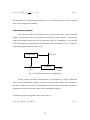
In a typical MSF plant shown in Fig. 2.5 we can distinguish between three basic
sections: heat rejection section, heat recovery section and the brine heater. On leaving
the first (warmest) rejection stage the feed stream is split into two parts, reject sea water
which passes back to the sea and a make up stream, which is then recycled back to the
flash section of the last stage. A recycle stream, which is drawn from the last stage,
passes through a series of heat exchangers, its temperature rises as it proceeds towards
the heat input section of the plant. Passing through the brine heater the brine
temperature is raised from the feed temperature at the inlet of the brine heater to a
maximum value approximately equals to the saturation temperature at the system
pressure. The brine then enters the first heat recovery stage through an orifice thus
reducing the pressure. As the brine was already at its saturation temperature it will
become superheated for a lower pressure and flashes to give off water vapor. The vapor
then passes through a wire mesh (demister) to remove any entertainment brine droplets
and onto a heat exchanger where the vapor is condensed and drips into a distillate tray.
The process is then repeated all the way through the plant as both brine and distillate
enter the next stage which is at a lower pressure. The concentrated brine is divided into
two parts as it leaves the plant, a blow-down, which is pumped back to the sea and the
recycle stream.
Reject Flow
Condenser tubes
Steam
Condensate
Sea water feed
Distillate
Distillate trays
Makeup
Flashing Brine
Recycle Brine
Brine Heater
Recovery section
Rejection Section
Fig. 2.5 Flow Sheet for the MSF process
45
Blowdown
2.6.2 The Process Model
The design and analysis
Stage j
TCj
TCj-1
of process operation requires the
use of a rigorous model of the
MSF plant.
A first principle
Dj-1
TDj-1
Dj
TDj
model for a 22 stages MSF plant
was developed and validated [2].
The specific plant consists of 3
Pj
Bj-1
TBj-1
Xj-1
Vj
Lj
rejection section stages and 19
Bj
TBj
Xj
Fig. 2.5b Single Stage
recover section stages. In the
following a summary of the developed model is given. Each plant stage is shown in Fig.
2.5b. The process is therefore defined by nine variables: brine pool height (Lj), brine
flow rate (Bj), salt mass fraction (Xj), brine temperature (TBj), distillate flow rate (Dj),
distillate temperature (TDj), coolant temperature (TCj), vaporization rate (Vj) and stage
pressure (Pj). Furthermore and in order to minimize the size of the model the liquid
levels, except that for the last stage, and the temperature dynamics in the distillate tray
are not included in the modeling. The dynamics for the salt concentration is also
excluded because they have no direct effect on the other process states except through
physical properties of the brine such as density and heat capacity. Our simulations
revealed that the physical properties vary between +1 and –1 % over the plant
temperature range due to changes in salt concentration. The mass holdup of the cooling
brine inside the condenser tubes is assumed constant. The following mass and energy
equations are written for each stage [2]:
Stage j (except the last stage)
• Mass balance of brine pool
ρ B , j AB
dL j
dt
= B j −1 − B j − V j
(2.71)
• Energy balance of brine pool
ρ B , j AB L j Cp B, j
dTBj
dt
= B j −1Cp B , j (TB , j −1 − TB , j ) − V j (λ c, j − Cp B , j (TB , j − To ))
(2.72)
• Mass balance in distillate tray
(2.73)
D j = D j −1 + V j
46
• Energy balance of condenser tubes
M C , j CpC , j
dTC , j
dt
= B0 CpC , j (TC , j +1 − TC , j ) + U j AHC ΔT j
(2.74)
U j AHC ΔT j = V j λ j
(2.75)
(for the rejection section the see water feed WF is used instead of B0 in (2.74))
Last stage, N
• Mass balance in brine pool
ρ B, j AB
dL N
= B N −1 − B N − V N + Wmk − B0
dt
(2.76)
• Energy balance in brine pool
ρ B , j AB LN Cp B , j
dTB , N
dt
= B N −1Cp B , j (TB , N −1 − TB , N ) − V N (λ N − Cp B , j (TB , N − To ))
(2.77)
+ Wmk Cp B , j (TC ,3 − TB , N )
• Mass balance in distillate tray
(2.78)
D N = D N −1 + V N
• Energy balance of condenser tubes
dTC , N
M C , N CpC , N
dt
= WF CpC , N (TF − TC , N ) + U N AHR ΔTN
U N AHR ΔTN = VN λ N
(2.79)
(2.80)
Splitter
WF = Rej + Wmk
(2.81)
Brine Heater
• Energy Balance equation
M BH Cp B, j
dTB 0
= B0 (CpC ,1TC ,1 − Cp B 0TB 0 ) + Ws λ s
dt
Additional relations:
47
(2.82)
In the above model equations the brine flow and the brine level in each stage are
correlated as follows:
(2.83)
B j = wL j K j ρ B , j ( P j −1 − P j + ρ B , j g ( L j − Ch j ))
Similarly, the distillate flow is correlated to the distillate level as follows:
(2.84)
D j = C D , j ρ D , j gL D , j
The temperature difference used in the above energy balances is defined as follows:
ΔTi = TB ,i − 0.5(TC ,i + TC ,i +1 )
(2.85)
Note that λj is computed at TBj while λc,j is computed at the distillate temperature, which
is assumed to be equal TBj minus the boiling point rise at the jth stage (BPRj). In the
original model [2-4], the physical properties for each stage in the above model, i.e.
ρ, Cp, λ, U , M c , M BH , BPR and the vapor pressure (P) are estimated through empirical
correlation.. Industrial values were used for the plant design parameters such as C, h,
AB, AHC, AHR and w. Moreover, realistic values for the size and number of tubes were
used in computing U, Mc and MBH. The definition of all parameters of the model
equations is given in the next table.
2.6.3 Process parameters and variables
Variable Description
Value
Units
1260
m2
AB
Cross sectional area for the brine chamber,
AHR
Heat transfer area for condenser tube at the rejection 7919.1
m2
sections
AHC
Heat transfer area for condenser tube at the recover 77314.8
m2
sections
B
Inter stage Brine flow rate
Calc
ton/min
B0
Recycle brine flow rates
217.257
ton/min
48
BD
blow-down flow rates
29.3
ton/min
C
Orifice contraction coefficient
0.625
CD
Discharge coefficient for the distillate tray
1.0
CpC,
Heat capacity for the brine in the condenser tube
Calc.
kJ/kg oC
CpB
Heat capacity for the brine in the flash chamber,
Calc.
kJ/kg oC
D
Distillate flow rate
Calc.
ton/min
g
Gravitational constant
9.8
h
Orifice height
0.11
K
Orifice discharge coefficient
0.68
L
Brine level
Calc.
m
LD
distillate level
Calc.
m
MC
Liquid holdup for the condenser tube
23654.0
Kg
MBH
Liquid holdup for the brine heater
34736.09 Kg
N
Total number of stages
22
P
Vapor pressure
Calc.
Bar
Rej
Reject flow rate,
95.35
ton/min
To
Reference temperature
0
o
C
TF
Sea Water feed temperature
35
o
C
TB
Brine temperature
Calc.
o
C
TC
condenser temperature
Calc.
o
C
C
C
m
Ts
Steam temperature
98.1
o
TB0
Top brine temperature,
93
o
U
Overall heat transfer coefficient for the condenser tube 35
kJ/min
o
Us
Overall heat transfer coefficient for the brine heater
49.5
C m2
kJ/min
o
C m2
V
Vapor rate, ton/min
Calc.
ton/min
X
Salt concentration
Calc/
kg/kg
WD
distillate product flow rate
19.2
ton/min
WF
Seawater feed flow rate respectively,
143.816
ton/min
Ws
Steam flow rate
2.452
ton/min
Wmk
Make up flow rate,
48.466
ton/min
w
Orifice width
0.5
m
49
wN
Orifice width for stage N
3
m
ρB
Density of brine
Calc/
kg/m3
ρD
Density of Distillate
1000
kg/m3
λ
Latent heat for vaporization,
Calc.
kJ/kg
λc
Latent
distillate Calc.
kJ/kg
Calc.
kJ/kg
heat
for
vaporization
at
the
temperature
λs
Latent heat for steam,
50
2.7 TWO CSTRs IN SERIES
2.7.1 Process Description and Flow Sheet
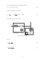
Consider two CSTRs in series with an intermediate mixer as shown in Fig. 2.6. A
chemical exothermic reaction of the form of: A Æ B takes place in the liquid phase. The
reaction rate is considered to be first order in the reactant species. The feed to the first
reactor is a pure species A with volumetric flow rate Q11 at ambient temperature. The
liquid inside the reactor converts partially to species B. The heat released from the
chemical reaction is removed by cooling water with volumetric flow rate Qcw1 and
temperature Tcw1. The outlet of the first reactor has a volumetric flow rate Q1 and
temperature T1, and it is mixed with a fresh feed of pure component A. The product of
the mixer is then fed to another reactor where the same first order reaction takes place.
Water at ambient temperature is also used to cool the second reactor. The outlet flow
rates are considered to be driven by the hydrostatic pressure in each tank, thus it related
to the square root of the liquid holdup inside the reactor.
Fig. 2.6 Flow Sheet for two CSTRs in series
2.7.2 The Process Model
The following modeling equations are taken from [7]. State variables are used to
describe the process variables. The definition of the states is given in section 2.7.3.
51
x&1 = Q11 − K v1 x1
(2.86)
x1 x& 2 = Q11 (C11 − x2 ) − K1 x1 x2
(2.87)
x1 x& 3 = K1 x1 x 2 ΔH + Q11 (T11 − x3 ) − UA1 ( x3 − x 4 )
(2.88)
V j1 x& 4 = Qcw1 (Tcw1 − x 4 ) + UA1 ( x3 − x 4 )
(2.89)
x& 5 = Q12 + K v1 x1 − K v 2 x5
(2.90)
x5 x& 6 = Q12 (C12 − x6 ) − K 2 x5 x6 + K v1 x1 ( x2 − x6 )
(2.91)
x1 x& 7 = K 2 x5 x6 ΔH + Q12 (T12 − x7 ) + K v1 x1 ( x3 − x7 ) − UA2 ( x7 − x8 )
(2.92)
(2.93)
V j 2 x& 8 = Qcw 2 (Tcw 2 − x8 ) + UA2 ( x 7 − x8 )
Additional relations:
K1 = k 0 exp(− E RT1 )
(2.94)
K 2 = k 0 exp(− E RT2 )
(2.95)
2.7.3 Process parameters and variables
Variable Description
Value
Units
C11
Feed concentration for component A
20
mole/m3
C12
Feed concentration for component A
20
mole/m3
E/R
Activation energy
600
K
Kv1
Orifice constant for valve 1
0.16
m3./2/s
Kv2
Orifice constant for valve 2
0.256
m3./2/s
k0
Pre-exponential factor
2.7x108
1/s
k1
Reaction rate in CSTR 1
1/s
k2
Reaction rate in CSTR 2
1/s
Q11
Feed rate for CSTR 1
0.339
52
m3/s
Q12
Feed rate for mixer
0.261
m3/s
Qcw1
Cooling water feed rate to CSTR 1
0.45
m3/s
Qcw1
Cooling water feed rate to CSTR 1
0.272
m3/s
T11
Feed temperature to CSTR 1
300.0
K
T12
Feed temperature to CSTR 2
300.0
K
Tcw1
Cooling water temperature to CSTR 1
300.0
K
Tcw2
Cooling water temperature to CSTR 2
300.0
K
UA1
Heat transfer coefficient times the heat 0.35
m3/s
transfer area for CSTR 1
UA2
Heat transfer coefficient times the heat 0.35
m3/s
transfer area for CSTR 2
Vj1
Cooling jacket volume for CSTR 1
1.0
m3
Vj1
Cooling jacket volume for CSTR 2
1.0
m3
x1
Liquid holdup in CSTR 1
4.4891016 m
x2
concentration of component A in CSTR1
0.0840220 mole/m3
x3
Temperature in CSTR1
362.99526 K
x4
Temperature of coolant in CSTR1
327.56042 K
x5
Liquid holdup in CSTR 2
5.4931641 m
x6
concentration of component A in CSTR2
0.0503550 mole/m3
x7
Temperature in CSTR2
362.99495 K
x8
Temperature of coolant in CSTR2
335.44732 K
ΔH
Heat of reaction
5
53
m3 K/mole
2.8 FLUID CATALYTIC CRACKING UNIT
2.8.1 Process Description and Flow Sheet
Fluid Catalytic Cracking (FCC) is one of the most important units in the
petroleum refining industry for the conversion of heavy gas oil to gasoline and light
hydrocarbons. The performance of the FCC units plays major role on the overall
economics of petroleum refineries. FCCU receives a number of hydrocarbon feedstreams with different molecular weight distribution from several refinery units and
cracks the heavier components in these streams to more valuable lighter ones.
Fig. 2.7 Flow sheet for FFCU process
The FCCU as Shown in Fig. 2.7 consists of two major processes; a reactor and a
regenerator. In the reactor, cracking reaction occurs and coke is deposited on the
catalyst. The reaction product is passed to the main fractionator for heat recovery and
separation into various product streams. The spent catalyst is sent to the regenerator
section where the coke is burnt by excess of oxygen to form carbon monoxide and
carbon dioxide. The gaseous products of the combustion reaction leave the regenerator
section through the cyclones as stack gas. The regenerated catalyst is recycled to the
reactor.
54
The catalyst is transferred back and forth between the reactor and regenerator
through the catalyst U-bend. Air is injected at the bottom of the regenerator lift pipe to
assist the circulation of the catalyst. Further detailed description of the process can be
found in [13].
2.8.2 The Process Model
The process dynamic equation can be found in the previous reference [13]. The model
equations are lengthy that we believe not to include them.
2.8.3 Process Parameters and Variables*
Variable
Description
Value
Cco
Concentration of carbon monoxide in 37
Units
Type
ppm
State/output
ppm
State/output
stack gas
CO2
Concentration of Oxygen in stack gas 0
Crgc
Weight
fraction
of
coke
on 0.0008475 ICFM
State/output
regenerated catalyst
Csc
Weight fraction of coke on spent 0.0078
ICFM
State/output
ICFM
algebraic
catalyst
Fsucca
Combustion air blower inlet suction 49465
flow
Fsucla
Lift air blower inlet suction flow
11750
ICFM
algebraic
Fsucwg
Wet gas compressor suction flow
19011
ICFM
algebraic
Fsurca
Combustion air blower inlet surge 45100
ICFM
constant
flow
Fsurla
Lift air blower inlet surge flow
9571.6
ICFM
algebraic
Fsurwg
Wet gas compressor surge flow
11700
ICFM
constant
Fair
Air flow rate into regenrator
75.5375
lb/s
algebraic
F1
Flow of wash oil to reactor riser
13.8
lb/s
input
F2
Flow of diesel to reactor riser
0.0
lb/s
input
F3
Fresh feed flow rate to reactor riser
126
lb/s
input
F4
Slurry flow rate to reactor riser
5.25
lb/s
input
F5
Fuel flow rate to furnace
34
lb/s
input
55
F6
Combustion air blower throughput,
60.9656
lb/s
algebraic
F7
Combustion air flow to regenerator
60.9656
lb/s
Algebraic
F8
lift air blower throughput
14.5719
lb/s
algebraic
F9
Combustion air flow to regenerator
14.5719
lb/s
algebraic
F10
spill air flow to regenerator
0.0
lb/s
algebraic
F11
Wet gas flow to the vapor recovery
mole/s
Algebraic
lb/s
Algebraic
lb/s
Algebraic
lb/s
Algebraic
lb/s
algebraic
lb/s
Algebraic
lb/s
Algebraic
1.1275
unit
Fv6
Flow through combustion air blower 60.1634
suction valve,
Fv7
Flow through combustion air blower 0
vent valve,
Fv8
Flow through lift air blower vent 0
valve,
Fv11
Flow through wet gas compressor 1.1275
suction valve
Fv12
Flow through wet gas compressor 0
vent valve
Fv13
Flow through wet gas compressor 0
anti-surge valve
Lsp
Level of catalyst in standpipe
10.1596
ft
Algebraic
n
Amount of gas
246.25
mole
state
Pblp
Pressure at bottom of lift pipe
32.1
Psia
Algebraic
P1
Combustion
suction 14.6421
Psia
State
surge 35.2159
Psia
State
air
blower
pressure
P2
Combustion
air
blower
pressure
P3
Lift air blower discharge pressure
40.5944
Psia
state
P4
Reactor Pressure
32.8244
Psia
algebraic
P5
Reactor fractionation pressure
23.3244
Psia
State
P6
Regenerator Pressure
29.6707
Psia
State
P7
Wet gas compressor suction pressure 22.4988
psia
State
Tcyc
Regenerator cyclone temperature
1279.2
o
F
State
992.6582
o
F
State
Tr
Reactor temperature
56
Treg
Regenerator bed temperature
1286.4
o
F
State
T1
Fresh feed temperature to furnace
460.9
o
F
Input
T2
Fresh feed temperature to reactor
667.2611
o
F
state
1607.6
o
F
State
T3
Furnace firebox temperature
V6
Combustion air blower suction valve 1
Input
position
V7
Combustion air blower vent valve 0
Input
position
V8
Lift air blower vent valve position
0
Input
V9
Spill air valve position
0
Input
Vl
List air steam valve
0.4313
Input
V11
Wet gas compressor suction valve 0.95
Input
position
V12
Wet gas flare valve position
0
Input
V13
Wet gas compressor vent valve 0
Input
position
V14
Stack gas valve position
0.612
Input
Wr
Inventory of catalyst in reactor
101696.89 lb
state
Wreg
Inventory of catalyst in regenerator
273763.07 lb
State
Wsp
Inventory of catalyst in regenerator 3200.27
lb
State
lb/ft3
State
spent pipe
ρlift
Density of catalyst in lift pipe
3.2
* definition and numerical values of various process parameters are given in the cited
reference.
The system has three major PI control loops which are set as:
Control loop
kc
τI
P4 Æ V11
0.1
0.04
ΔP Æ V14
0.08
0.03
Fair Æ Vl
0.01
0.0025
57
The process has several equipment and operational constraints as follows:
Flows:
0 ≤ F1 ≤ 17
0 ≤ F2 ≤ 16
0 ≤ F3 ≤ 144
0 ≤ F4 ≤ 10
0 ≤ F5 ≤ 20
Valves:
0 ≤ Vi ≤ 1;
i = 1,14
Vessels:
P6 < 39.7 psig
P5 < 39.7 psig
Compressor surge limit (level: 10)
Lift air:
Fsuc – Fsur > 0
Combustion air
Fsuc – Fsurg > 0
Wet gas
Fsuc – Fsur < 0
Total combustion in regenerator (level: 9.5)
CO,sg > 1.5%
Treg > 1265 oF
Or
Tcyc – Treg < 20 oF
Tcyc < 1310 oF
CCO,sg < 350 ppm
58
Differential pressure: (level 8)
–5.0 ≤ ΔP ≤ –2.0 psi
Standpipe level: (level lower limit = 10, upper limit = 8)
0 ≤ Lsp ≤ 20 ft
Riser Temperature: (level 10)
Tr ≤ 995 oF
Furnace Temperature: (level 9)
T3 ≤ 1700 oF
59
CAHAPTER 3: THEORETICAL BACKGROUND
3.1 INTRODUCTION
As mentioned in Chapter 1 and 2, PCLAB deals with exercises that deal with
steady state and dynamic analysis of the process. The analysis is essential part of the
controller design. In this chapter, the reader will be introduced to some of the terms that
will be encountered in most of the exercises to be performed.
The modeling of industrial processes usually starts with a balance on a
conserved quantity mass or energy. Mass and energy balances are very important for the
engineer to describe the process mathematically. This balance can be written as:
Total flow rate of
(mass/energy)
the system
Total
flow
rate
of
Accumulation rate of
into – (mass/energy) out of the =
system
(mass/energy) within (3.1)
system
As we can imagine, in writing these balances and all other auxiliary equations,
we must make use of almost every area of process engineering, such as
thermodynamics, heat transfer, fluid flow, mass transfer, reaction engineering, etc. This
makes the modeling of industrial processes most interesting and challenging. After
characterizing the system by the model, it is then necessary to analyze the behavior of
the system in terms of its variables that affect the controlled parameter, or the effect of
disturbances that surface to affect the controlled parameter with time. When these
variables are known, steps are then taken to keep them in check through the
development of control algorithms.
Applying (3.1) usually results in nonlinear ODE equations which can be
linearized and converted into transfer function in the form of:
y ( s) =
First Order with Dead Time (FODT):
60
ke −θs
u(s)
τs + 1
(3.2)
y ( s) =
Second Order with Dead Time (SODT):
ke −θs
u ( s)
τ 2 s 2 + 2ζτs + 1
(3.3)
3.2 STEADY STATE ANALYSIS
From (3.1), we conclude that the analysis of a process control system requires an
understanding of the overall system behavior and the reflection of this behavior in the
properties of the system elements. These properties are highlighted during steady state
conditions where, the accumulation term in the above equation goes to zero. The state
variables do not change with time and the input is then directly related to the output.
This leads to the definition of the steady state gain as:
K=Change in output/Change in input
(3.4)
This relation is useful to determine the effect of manipulated and load variables
on the controlled variable of a process. Thus the relation characterizes the effect that a
change in an input variable has on an output variable. Implicit in this characterization is
the fact that changes in the controlled variable can be calculated by summing up the
changes in all the manipulated and load variables multiplied by a constant gain
coefficient. This superposition applies only to linear systems. Steady state models are
frequently used to determine set points for controllers whose measured variables are
dynamic multiple-input computed variables. They are used to adjust the set points of
unit operations performance variable..
3.2.1 Steady State Disturbance Sensitivity Analysis
Steady state disturbance analysis is a tool developed by (Yi and Luyben, [17]) to
study the controllability and further the control structure of a given process. It is more
suitable for nonlinear processes where the effect of process disturbance on the plant
steady state operating condition is investigated.
Steady State disturbance sensitivity analysis can be carried out in two modes:
Open loop
Closed loop
61
In the open loop mode, steady state disturbance analysis illustrates how much a
chosen process output changes at steady state for various different values of a given
disturbance when all the manipulated variable are fixed at their corresponding steady
state values. In this case, the severity and nonlinearity of the disturbance impact on a
certain process output can be investigated. Moreover, one can compare the effect of the
designated disturbance on several process outputs and find out which one is the most
influenced.
In the closed loop mode, the steady state disturbance sensitivity analysis (ssdsa)
demonstrates how much a specific input or a group of inputs should change to keep a
controlled output or group of controlled outputs at its set point at steady state for
various values of a given disturbance while the other inputs are fixed. Given certain
constrains on the inputs, one can select the most appropriate input to regulate a specific
output under the influence of a particular disturbance.
The steady state disturbance analysis (SSDA) is obtained by solving the static
version of the process model for different values of a pre-specified disturbance with a
set of particular outputs and all the inputs, except those used as manipulated variable,
are fixed. The numerical solution is carried out using fsolve m-function of MATLAB.
Further discussion and analysis of this tool will be discussed in a later chapter.
3.3 DYNAMIC ANALYSIS
The word dynamic conveys the idea of a time variation which can result from a
number of unspecified or unknown influences; the word variable simply relates the
capacity to vary from these influences. In process control we are interested in those
dynamic variables which require regulation in some industrial application. Typical
examples are: temperature, pressure, flow rate, level, force, light intensity, and
humidity. Dynamic analysis can be performed in open-loop model and closed-loop
mode.
3.2.1 Open-loop Dynamic Analysis
In open-loop dynamic analysis no control algorithm is involved. Therefore the
dynamic response of a process variable to forced input variation can be studied.
62
Dynamic response is a measure of the systems reaction, as a function of time, in
correcting transient inputs, or adjusting to a new set point. In this case, the dynamic
analysis is useful to understand the dynamic behavior of a process and to characterize
the process dynamic parameters such as time constant, damping factor, period of
oscillation and dead time.
When a FODT process is subject to a step change in its input variable, it
responds as shown in Fig. 3.1. The output reaction can be recorded and plotted to infer
the system parameter. The figure shows how estimate the gain, time constant and dead
time directly from the transient response. This procedure is known as reaction curve
method.
Fig. 3.1: Output response for a step change for first order system, (a) with time delay,
(b) without time delay
Accordingly, the time constant is estimated directly from the response curve while the
static gain is simply:
k=
Δx
Δu
(3.5)
63
Similarly, when the input variable is stepped, the output of an under-damped
second order system responds as shown in Fig. 3.2. From the recorded data, it is easy to
identify the system parameters as follows:
Static gain: k =
xss
Δu
Damping ratio: solve
A
B
= exp(
Natural period of oscillation: τ =
− 2πς
ψ
for ζ .
)
Tψ
2π
Where ψ = 1 − ς 2
Fig. 3.2: Output response to a step change for second order system
3.2.2 Closed-loop Dynamic Analysis
The evaluation of system performance simply reflects the ability of a process
control loop to regulate some dynamic variable in the process. Such regulation is
specified through two criteria. The first criterion is the system error of the system in
maintaining the controlled dynamic variable at the specific value defined by the set
64
point CSP .The second criterion is the dynamic response of the system to any disturbance
of the process or change of the process control loop set point.
The system error is a measure of the inherent error between the system set point
value and the actual value of the dynamic variable maintained by the system. The
desired value of the dynamic variable in the process is referred to as the set point.
Generally, a set point CSP is expressed with some allowable deviation ± ΔC
about the nominal value. Thus, when control has been achieved the actual value of the
dynamic variable may be in the range from (CSP – ΔC) to (CSP + ΔC). Of course the
wider the allowable deviation the easier the control is to achieve. Note that this
deviation can never be less than the inherent system error.
Feedback control loop
The regulation of a specific dynamic variable is usually carried out in feed back
fashion as shown in fig. 3.3.
Fig. 3.3 Typical Feedback control configuration
The feedback controller is the component of the feedback loop that issues
control commands to the process (via the final control element) based on e, the
deviation of the process measurement from its desired set point value. The way the
controller calculates the type of command signal to be issued for any given value of e is
what differentiates one controller from another. To consider all dynamic elements of a
feedback controller, the following block diagram is usually used:
65
Fig. 3.4 Typical Block diagram for Feedback Control
According to fig. 3.4, the following are defined:
Gc(s) = controller transfer function.
Gv(s) = final control element (valve transfer function).
Gp(s) = process transfer function.
Gd(s) = disturbance transfer function.
Gm(s) = measurement device transfer function.
C(s) = controller signal.
ym(s) = measured output.
ysp(s) = set point.
e(s) = error .
PID controller
The operating equation for PID controller is:
⎡
1
C (t ) = K C ⎢ e (t ) +
τI
⎣
t
∫ e ( t ) dt + τ
0
D
de ⎤
⎥ + CS
dt ⎦
(3.6)
Taking Laplace transform of the above equation we get:
⎛
⎞
1
+ τ D s ⎟⎟ e ( s )
C ( t ) = K C ⎜⎜ 1 +
τIs
⎝
⎠
(3.7)
The transfer function for PID controller is:
66
⎛
⎞
1
G C ( s ) = K C ⎜⎜ 1 +
+ τ D s ⎟⎟
τIs
⎝
⎠
(3.8)
The parameter Kc is called proportional; gain, τD is called the derivative time constant
and τI is the integral time constant.
Feed-forward system
The objective of the feed-forward control is to keep the values of the controlled
output as its defined values. It is configured such that predictive action is taken on the
controlled variable, thus it does not wait until the effect of a disturbance is already felt
in the system but acts appropriately in anticipation of the disturbance. Fig. 3.5 depicts a
typical feed forward control element [16].
Controller
Manipulated
variable
Disturbance
Process
Controlled
variable
Fig. 3.5 Feed-forward Control configuration
In this control, the direct measurement of a disturbance is used to adjust the
values of the manipulated variable to achieve a desired output value. The controller is
the active element that receives the information from the measured parameter and takes
appropriate action to adjust the values of the manipulated variable.
Consider the open-loop systems to be in the form of:
y ( s) = G p ( s)u ( s ) + Gd ( s )d ( s )
(3.9)
67
Let ysp be the desired set point for the controlled variable:
y sp ( s ) = G p ( s )u ( s ) + Gd ( s )d ( s )
(3.10)
The feed forward controller is therefore:
⎡ 1 sp
⎤ G (s)
≡ Gsp y sp − d ( s ) Gc
u ( s) = ⎢
y − d ( s )⎥ d
G
(
)
G
s
⎣ d
⎦ p
[
]
(3.11)
And the block diagram with FFC looks:
d
ysp
_
Gsp
+
Process
Gc
Gd
+
Feedforward control
mechanism
GP
+
y
Fig. 3.6: FFC block diagram
Therefore,
Gsp =
1 τds +1
=
Gd
kd
(3.12)
Gc =
Gd kd τ p s + 1
=
Gp k p τ d s + 1
(3.13)
68
Cascade Control
A cascade or multi-loop control is a way of minimizing a disturbance that enters
a slow process. It has two sets of controllers, a primary and a secondary. Instead of
adjusting the final control element such as a valve, the output of a primary controller is
the set point of a secondary control loop. Thus cascade control uses the output of the
primary controller to manipulate the set-point of the secondary controller as if it were
the final control element. The block diagram for a cascade controller is shown in Fig.
3.7[16].
r1
+
_
r2
GcI
+
_
GcII
v
GpII
dII
+
y2
+
GpI
dI
+
+
y1
Secondary Loop
Primary Loop
Fig. 3.7 Cascade control configuration
The reasons for using this type of control are as follows:
•
Allow faster secondary controller to handle disturbances in the secondary loop.
•
Allow secondary controller to handle non-linear valve and other final control
element problems.
•
Allow operator to directly control secondary loop during certain modes of
operation (such as startup).
Requirements:
Secondary loop process dynamics must be at least four times as fast as primary loop
process dynamics.
•
Secondary loop must have influence over the primary loop.
•
Secondary loop must be measured and controllable.
Cascade control can be used when there are several measurement signals and one
control variable. It is particularly useful when there are significant dynamics, e.g. long
dead times or long time constants between the control variable and the process variable.
69
CHAPTER 4: STEADY STATE DISTURBANCE SENSETIVITY
ANALYSIS
4.1 INTRODUCTION
In this chapter we discuss how steady state disturbance analysis can be
implemented on PCLAB. This procedure is very useful to design the appropriate control
structure. When controlling a plant or a process with many inputs and outputs, it is
usually difficult to optimally pair theses variables into multi single loops structure.
SSDA is a tool that can help in this regard, however it can not be implemented on real
plant. Instead simulation can be utilized to perform the task.
Referring to the menu of the Evaporator case study in Fig. 1.16, clicking on the
“steady state disturbance analysis” button brings up the following window:
Fig. 4.1 Steady State Disturbance Module for Evaporator Process
Fig. 4.1 shows that the process has three inputs and four possible disturbances.
The procedure will focus on investigating the static effect of any disturbance or any
combination of disturbances on the process outputs in open-loop mode. This means that
the inputs will remain fixed during the test. This is known as the open loop test. It
70
reveals which process output is affected the most and which one is affected in nonlinear
fashion. One can also run the test in closed-loop mode. In this case, an output should be
selected as the controlled variable and a corresponding input should be selected to be
the manipulated variable. The test will then examine the effectiveness of the chosen
input to maintain the controlled variable at its nominal value in steady state when the
process is under the influence of a range of disturbance values.
To start the procedure, one can simply click on the green button or the start
button on Fig. 4.1. By doing so, the following SSAD menu pops up:
Fig. 4.2 SSDSA menu for the evaporator process.
The menu in Fig. 4.1 has six steps that lead to carry out the SSDA analysis
procedure as discussed in the following sections.
4.2 OPEN-LOOP MODE
First the user should select one of the four possible disturbances by marking the
appropriate check box. Let us say the feed temperature. Note that the other case studies
will have different list of disturbance variables. Next mark the open-loop check box.
The third step controls the test range. For example, if the nominal value for the feed
temperature is T0 = 40 oC and using step size of 0.1 and number of steps of 10 then the
disturbance value will have the following range during the test:
71
Increasing the number of steps at the same step size will increase the
temperature range to be covered. The above values for the step size and number of steps
cover a ±50% range which is good enough from practice point of view. Decreasing the
step size will help in producing smoother response curves but it will decrease the
overall range. Therefore, if one decreases the step size for better resolution, he should
also increase the number of steps to maintain the same operating range. It should be
noted though that smaller step size requires higher computational load.
In the open-loop mode, steps 4 and 5 must be by passed. If you by mistake
marked one of the boxes in step 4 or 5 , you will receive an error message which will be
displayed in the warning box. Now press the run button and look at the results shown in
Fig. 4.3.
Fig. 4.3 SSDSA results for open loop test.
Fig. 4.3 illustrates how the four main process outputs respond at steady state to
changes in the feed temperature from 20 to 60 oC. It is obvious that the liquid level in
the separator unit is not affected by this type of disturbance. Thus in the open loop
mode, the user can gain information about the directional, magnitude and nonlinearity
effect of a disturbance. For example as a directional effect, both C2 and P2 will increase
when the feed temperature increase while the outlet flow rate F2 will decrease. One can
also observe that the solute concentration (C2) received the highest (magnitude) impact.
Moreover, all outputs are altered linearly with the temperature variation. Thus, the user
72
can learn how the process operation and product quality may get seriously influenced
when the feed temperature is changing freely.
Fig. 4.4 SSDSA menu for the closed-loop test case
4.3 CLOSED LOOP MODE
In this test mode, the user should unmark the open-loop checkbox and mark the
close-loop checkbox instead. Furthermore the user needs to specify a controlled
variable. Let us choose for example the output concentration C2. In addition, the user
should select one of the manipulated variables listed in Step-Box 4 as the candidate one.
Let the candidate manipulated variable be the coolant flow rate. The user has the choice
to either change the upper and lower permissible values for the candidate manipulated
variable or leave them at their default values. See for example Fig. 4.4. Note that the
user can restore the default values for the upper and lower limit any time by simply
clicking the “reset limit” button.
After the user finishes marking the required checkboxes in the SSDSA menu, he
can simply click the run button in Step-Box 6. The result for the above specification is
shown in Fig. 4.5.
73
(a)
(b)
Fig. 4.5 Output responses to disturbance in feed temperature when the coolant flow rate is
used as manipulated variable
By inspecting the output response in Fig. 4.5a, we can observe that the
controlled variable C2 is well maintained at the nominal value. Note that a red color is
used for the controlled variable to distinguish it from the other uncontrolled outputs.
Because the evaporator pressure is not controlled, it increases as expected with
disturbance but this time with a larger magnitude. On the other hand, the feedback
control helped in making the output flow rate changes slightly with disturbance.
More important is the response of the manipulated variable. The red lines in the
right plot of Fig.4.5b shows the upper and lower limits for the coolant flow rate which is
set at 400 and 100 respectively. The white line represents the response of the coolant
flow rate to disturbances in order to maintain C2 at nominal value. For large
disturbances, i.e. when the feed temperature exceeds 55 oC, the coolant flow should be
reduced slightly below the lower limit in order to reject the effect of the disturbance.
However, at feed temperature below 30 oC, the coolant flow rate must be increased by
many folds, especially below 25 oC, to maintain the required operation. Low feed
temperature requires higher steam pressure to provide enough heat of evaporization
which in turn increases the process temperature. As a result large amount of coolant
flow is needed to absorb the extra heat and to cool down the vapor.
74
One can conclude that the coolant flow rate is a good manipulated variable for
controlling the product concentration at moderate to high disturbances in the feed
temperature. However, the coolant flow is recommended at low feed temperature. The
user can test other candidate manipulated variable and can also repeat the procedure for
the other controlled variables. At the end, the user can build up a satisfactory control
structure for the process, i.e. can select the appropriate input-output pairing
configuration.
The SSDSA can be studied for each loop individually and consequently the
appropriate structure can be determined. This approach however ignores the cross loop
interaction. Alternatively, one can conduct the SSDSA method over all process
variables and determine the best design structure
75
CAHAPTER 5: OPEN-LOOP DYNAMIC ANALYSIS
5.1 INTRODUCTION
Of the seven systems that were defined in chapter 2, some follow the response of
first order systems, others follow that of second order systems and yet others follow
those of higher order systems. In this chapter we will practice the responses of some of
these systems to input manipulations or disturbances. The response of an output
parameter to changes in an input parameter with time is referred to as system dynamics.
Normally the input parameter must behave in a certain defined fashion like step, ramp
or sinusoidal.
As discussed in the previous chapter, dynamic analysis can be performed on an
open-loop model as well as on a closed-loop model. For systems that mimic first order
dynamics, system parameters like gain, time constant and dead time can be computed.
These parameters are typical to system response to a step change in the input
Here, it is intended to perform the computations of these parameters using the
PCLAB software described in chapter one. This will provide a hands-on application and
will enable the reader to calculate the parameters that characterize the system.
5.2 FIRST-ORDER SYSTEM’S DYNAMIC ANALYSIS
In order to run the software, recall how you were instructed to lunch PCLAB in
chapter one. Follow the same steps till you arrive at Fig. 1.13. Using the main menu of
this figure, choose the Forced Circulation Evaporator to get Fig. 1.16, and then from
this menu choose the first item on the menu to get Fig. 5.1.
Fig. 5.1 shows the open-loop configuration of an evaporator process. The blue
colors to the left indicate input parameters. There are seven of them as defined in the
chapter on modeling. These include temperature, flow rates, pressure and the
concentrations defining the process. The red-colored items to the right represent the
output parameters that are important to process performance. These four parameters
represent the level, pressure, flow and concentration for the evaporator. The yellow
portion in the middle, represent the process itself. Observe the green icons on the
76
top left, one of which can take you back to the menu and the other to the interactive
graphic tool. The coloration code is typical for all the case studies available in the
software.
Fig. 5.1 Open Loop Evaporator Process menu
Double clicking on any of the input boxes, will give you access the seven inputs
described earlier. For instance, if you need to make a change on the feed flow rate to
the evaporator, double click on the third input box, designated by F1. A Block
Parameter window will appear, as shown in Fig. 5.2.
Fig. 5.2 Block Parameter window for feed flow input
77
Note that the current flow rate is 10 kg/min. To change this number simply use
the mouse to highlight the number 10 by right clicking the mouse, hold and drag
slightly to the right until the number 10 is fully highlighted, then release the mouse.
Now type in the number 11 and press the OK button. This way, a 10% step increase
in the inlet flow is attributed to F1.
After effecting this change, press on the run icon or press simulation and then
start. Note that in this case the 300 seconds allotted may not be enough, so click on
Simulation then Parameters to get Fig. 4.3. Using the parameter menu option (see
Appendix A.3), the stop time of this run should be changed from 300 seconds to 400
seconds. This will enable you to capture enough time for steady state operation. Use
the same procedure as in changing the value of the Block Parameter window,
change the run time from 300 to 400 seconds.
Now run the simulation by pressing on the start button in the simulation menu.
After the 400 seconds has elapsed, the run will be complete. Click on the first output
icon for level to view Fig. 5.4. The input has changed step-wise from 10 to 11
kg/min. The output response of the tank to this change is seen to rise steadily to
attain a new steady state value. Observe the dead time represented by the flat portion
of Fig. 5.4. In this region, the liquid height in the tank does not change with time. In
order to read the numerical value of the time during which the system stayed flat,
choose the first icon on the top left. Click this icon to allow you enlarge the scale
and read the corresponding value on the x-axis as shown in Fig. 5.5. The enlarged
portion shows the output response beginning after 10 seconds.
78
Fig. 5.3 Simulation Parameter window for stop time change
Fig. 5.4 Output showing the height of tank versus time
The region or period is known as the dead time during which the system does not
respond to any input change or disturbance. One can then use the plot of Fig. 5.4 to
calculate the process gain and the time constant as per (3.2) and (3.3).
79
Fig. 5.5 Part of Output showing the height of tank versus time
The gain is defined as the change in output over the change in the input. This
ratio is given by (5.1) for the liquid level
Lss − L0
F2 − F0
(5.1)
Where L0, is the initial level of the tank and Lss the final tank level. F0 is the
initial flow and F2 the final flow.
This gives a value of 0.089 m-min/kg as the steady state gain. This value of
the gain tells us that the for a ten percent change in the input flow rate the liquid
level in the storage tank of the evaporator process will change by about 9 percent.
Or for a unit step change in the input the tank level will increase by 0.089m.
Similarly, the time constant, τp, of the process can also be calculated from the
graph. Refer to Fig. 3.1 to refresh your memory on some of these calculations. To
do this calculation, the change in the output from the initial steady state to the final
steady state value is calculated through (5.2) below.
ΔL = Lss − L0
(5.2)
80
ΔL, is calculated as (1.05-0.961) to get 0.089m. Now apply (5.3) to get the level of the
tank at one time constant.
Lλ P = L0 + 0.632* ΔL = 1.017248
(5.3)
Double click on the first red output icon to revisit Fig. 5.4. Then use the icon
with binoculars to auto-scale your plot. Now use the three zoom options to the top left
of your plot to vary the y-axis until you read the height of 1.017m. Note the
corresponding reading on the x-axis as 46.5 seconds. This gives you the value of λp for
the process.
Now look at the output concentration icon by double clicking on it. Enlarge the
graph to obtain Fig. 5.6. Notice how the concentration response falls rapidly to a new
level of concentration as against the rise in the level of the tank. Using the same
methodology, the gain for the concentration icon was calculated as –7.03 %-min/kg.
This means for a unit step change in the input flow, the concentration falls seven
percentage points. From this it is clear that process gains can be negative. The time
constant was calculated as 17.05 seconds. The concentration response is therefore seen
to be 2.7 times faster than the level response.
Table 5.1 Calculated values of the characteristic parameters for positive step change
Kp
τp
td
0.089
46.5
10
Concentration -7.03
17.05
10
Pressure
-0.4472
46.2
10
Flow
0.033
37.5
0
Level
Table 5.1 was generated for all the four output parameters that were calculated
using the procedure above. The graphs of the outputs were plotted separately and the
81
values of Kp, , τp and td were all calculated from the graphs based on 10% change in
the input flow.
Fig. 5.6 Output showing the change in concentration with time
If Kp is large the system becomes very sensitive and a small change in the
input forcing function will result in a very large response. The output concentration
has the largest gain and therefore a small change in the input flow will result in a big
change in the concentration. On the other hand, The outlet flow has the smallest
gain of 0.033, so if large changes are made in the input flow, the outlet flow will not
be unduly disturbed. It is possible for the gain parameter to be negative. If it is
negative, then the next steady state value will be lower than the initial steady state
and the curve will be seen to fall to the new value as in the cases of pressure and
concentration. However, if the gain is positive, then the response curve rises and
settles at a higher new value.
The time constant, is a measure of how fast a particular parameter responds to
an input forcing function. The concentration parameter has the smallest time
constant and therefore it is the most sensitive to changes in the inlet flow. The
pressure and the flow both respond within the same magnitude of time.
82
All the parameters show the same value for the dead time except the outlet
flow. This is the time it takes before the parameters start or begin to respond to the
forcing function. Probably, this dead time is inherent in the system.
The analysis can also be done by storing the raw data to a workspace which
could be used in other software like EXCEL or the MATLAB itself. To achieve this,
double click the output icon whose data you wish to store before starting the run.
For instance, if you wish to store the data of the level in the tank, then double click
the first output icon of Fig. 5.1. Doing so will open for you the window similar to
Fig. 5.4 but without any plots. Then click on the sixth icon on the top left
(Properties). Next, click on the Data History icon to get Fig. 5.7.
Now, mark the box of ‘Save data to workspace’ and give it a variable name. Choose
“Matrix” for Format box. Click on ‘Apply’ or ‘OK’ to continue. Make your run or
simulation as described earlier and continue. The stored data can be viewed on
MATLAB command window by typing the variable name at the prompt option of
MATLAB. The data will be stored in MATLAB workspace as a matrix under the
chosen variable name. the data can be saved for further analysis or plotting.
Fig. 5.7 Level Properties window for saving data to a workspace
5.2.1 Nonlinearity Analysis
Approximating the process dynamics by a first order system is based on that
assumption that the physical process responds linearly to input variation. However,
83
this is not true for most chemical processes except at a very narrow operating
region. Therefore, it is necessary to use small process perturbation in order to obtain
faithful process parameters, i.e. static gain and time constant. However, the input
perturbation should be large enough to create reasonable signal to noise ratio. In this
sense, the appropriate procedure for identifying the process parameters is a trial-anderror. This will be explained in the next paragraphs.
Now, let us see what happens when the step change is –10%. This is done the
same way by invoking the Block Parameter of F1 and changing the flow rate from
10 to 9 kg/min. Fig. 5.8 is the graph for the response of the tank to the input forcing
function. From the graph, there is an immediate inverse response before the curve
picks up to respond normally. Similar to the previous paragraph, the parameters of
this run are captured and listed in Table 5.2
Fig. 5.8 Output showing the height of tank versus time
Table 5.2 Calculated values of the characteristic parameters for negative step change
Kp
τp
td
-0.05
111.2
10
Concentration -20.1
28.8
10
Pressure
0.26
116
10
Flow
-0.0235
118
0
Level
84
Table 5.2 still shows the concentration output parameter to be the most
sensitive with a time constant of 28.8 seconds. The gain is seen to be very high
reaching 20.1 % for a step change of –10 %.
The gain and the time constant
parameters in Table 5.3 are different from those in Table 5.2 and 5.1 for an input step
change of 10% and –10%. It should be noted that the dead time was not affected by
the step change because it is intrinsic property of the process. Moreover, the dead time
incorporated by ad hoc method.
For linear systems, the process parameters must have the same absolute
magnitude for the same magnitude of step change. Therefore the systems dynamics
for 10% step change do not exhibit linearity in that region. Since linearity is the
basis of these calculations, further tests need to be carried out to establish the
existence of linearity. One can also check the process linear behavior through testing
the plant for step changes of specific proportional magnitudes. In this case, the
calculated process parameters should have the same proportional magnitudes.
Otherwise the process is said to behave nonlinearly.
Table 5.3 Comparison of the values of the characteristic parameters
Kp
τp
td
+10% step change
0.089
46.5
10
-10% Step Change
-0.05
111.2
10
In order to establish this linearity, the step changes were reduced by ten orders
of magnitude. Instead of an increment of 1 kg/min on the flow rate, an increment of
0.1 kg/min was made. The module is simulated and the corresponding process
parameters were estimated as shown in Table 5.4. The step change was then doubled
to an increment of 0.2 kg/min. using the same procedure outlined above, Table 5.4
was produced. In this region an approximation of linearity can be assumed because
the values of the gains are close to each other at 0.058 and 0.06 m-min/kg
respectively, while the time constants are also close to 30 seconds.
85
Table 5.4 Calculated values of the characteristic parameters for 1% step change.
Step Change Step Change
0.1 kg/min
0.2 kg/min
L0
0.9604
0.9604
Lss
0.9662
0.9729
ΔL
0.0058
0.0125
0.632ΔL
0.00367
0.0079
L0 + 0.632ΔL
0.9641
0.9683
Lτ
0.9641
0.9683
τ
27.6
30
Kp
0.058
0.06
5.3 SECOND ORDER SYSTEM DYNAMICS
Let us now look at the open-loop response of second order systems. These
systems are known to have differential equations of the form given in (3.3). The
Laplace transform of this differential equation yields a second order transfer function
given by the equation below.
y(s)
Kp
= G(s) = 2 2
u(s)
τ s + 2ζτ p s + 1
(5.4)
Where:
y(s) is the system output
u(s) is the input forcing function
Kp is the system gain
τp is the natural period of the system
ζ is the damping coefficient
Second order systems occur in nature. Such systems are said to be inherently
second order. They can be derived from a multi-capacity system, such as two first
86
order systems in series through which material or energy flow. Many closed-loop
systems also exhibit second order behavior.
In this chapter, the dynamic behavior of these systems is to be studied based on
step changes in the input forcing function. When there is an input forcing function, the
response of these systems follows that of the transfer (5.4). The key parameter of this
equation is the damping factor. Depending on the value of the damping factor, the
system can be overdamped, critically damped or underdamped.
Fig. 3.2 shows a typical output response of an under-damped second order
system to a step change in the input. From the data generated by simulating the
system, its characteristic parameters can be calculated as shown in the Figure.
In this case, the Polyethylene Reactor example is to be used to make the
necessary parametric calculations. To do this, revisit Fig. 1.13 and choose the
Polyethylene example on the menu by clicking on it to get Fig. 5.9. The figure shows
the Polyethylene Process Menu. Choose the second item on the menu (Polyethylene
(stable)) by simply clicking on it. This leads to the process flow sheet of the
polyethylene process as shown in Fig. 5.10. Remember, the coloration code discussed
earlier still applies.
Fig. 5.9 Polyethylene Process Menu
87
Double click on the input parameter of the recycle flow rate Fg, to obtain the
Block Parameter icon. Then increase this recycle flow from 8500 to 9020 moles/s. After
this is done, close the Block parameter icon for the recycle and double click that for
hydrogen flow, FH to obtain Fig. 5.11. Once this is displayed on your screen use the
keyboard to enter 2.2 moles/s instead of the 1.16. Press the enter button for the system
to accept this entry. Now, run the simulation as the same way it was done in the first
part of the chapter. When the run button is pressed, PCLAB will run your simulation
based on the values of the new parameters that were entered.
Fig. 5.10 Process Flow Diagram of the Polyethylene system
After the run is complete, double click on the last red icon to the right of your screen,
the temperature T, to get Fig. 5.12. The graph shows the plot of output bed temperature
versus time for a typical second order system. The nature of the graph resembles that of
Fig. 3.2. Applying the definitions used in the Figure, A is found by subtracting the
steady state height (T) from the maximum reading of 122.65 oC as shown in Table 5.5.
B is similarly calculated as the ultimate value of the response. Then the ratio of A/B
gave the overshoot. The period is also calculated by taking the time elapsed between
two consecutive crests. Using the equations and the appropriate figures of Chapter 3,
Table 5.6 was generated. The overshoot is the ratio of the maximum amount by which
88
the response exceeded its ultimate value to the ultimate value of the response. It is
related to the damping factor through the equation shown in the Table. It increases with
decreasing ζ and as ζ approaches 1, the overshoot takes the value of zero and the
system response is described as being critically damped.
Fig. 5.11 Block Parameter for hydrogen flow, FH moles/s
Fig. 5.12 Simulation Results of the Open Loop Polyethylene Reactor.
The system seems to have a very large time constant of 11515 seconds. The
static gain of 26.5 seems to be equally large. This shows that the system has very large
capacitance. Good design engineers are able to reduce these parameters so that the
system can have quick response.
Other parameters that can be calculated from the graph are the rise time and the
response time. Since the system took a response time of 2.29x105 seconds to reach its
ultimate value with equally large value of the rise time (found to be 22,200 seconds),
then the system is expected to have large capacitance. The system seems to have a very
large time constant of 11515 seconds. The static gain of 26.5 seems to be equally large.
89
This shows that the system has very large capacitance. Good design engineers are able
to reduce these parameters so that the system can have quick response.
Other parameters that can be calculated from the graph are the rise time and the
response time. Since the system took a response time of 2.29x105 seconds to reach its
ultimate value with equally large value of the rise time (found to be 22,200 seconds),
then the system is expected to have large capacitance.
Table 5.5 Calculated characteristic parameters for the Polyethylene Process
Parameter
Equation
Value from Graph
A
122.65-99.9
22.75
B
99.9
99.9
OVERSHOOT
A/B
0.2277
DECAY RATIO
(OVERSHOOT)2
.0519
4
87600
4
T2
8.76*10
T1
1.52*10
15200
T
T2-T1
72400
Tn
ζ
τ
Kp
Tψ
11515
2π
exp(
−2πς
ψ
0.03621
)
Tψ
11515
2π
xss
Δu
26.5
Remarks:
•
The green box labeled “Go to menu” shown in the Simulink Module can be used
to switch between the active Simulink module with the current active sub menu.
•
The green box labeled “graphical tool” shown in the Simulink Module can be
used to trigger the plotting forum. The usage of the plotting forum is discussed
in Appendix A.
90
CHAPTER 6: CLOSED-LOOP DYNAMICS
6.1 INTRODUCTION
A closed-loop system normally has a controller together with other hardware
components, but the key component here is the controller. The closed-loop response
also depends on the transfer function of the system and on the nature of the change.
Normally the change is divided into two, namely, set point and disturbance. If there is a
set point change, the feed back controller acts in such a way as to keep the ultimate
response as close as possible to the changing set point. On the other hand, if there is any
form of disturbance but the set point remains the same, then the feed back controller
tries to eliminate the impact of the disturbance or load changes and keeps the ultimate
response at the desired set point. However, the presence of other hardware components
could lead to oscillatory behavior and unstable systems. Therefore it is important to
design controller systems that will eliminate all the instability.
6.2 CONTROLLER TUNING
Performance of feedback controllers depends on the values of their chosen
parameters. If these parameters are properly chosen, they offer the highest flexibility to
achieving the desired controlled response and stability. The process of choosing these
parameters is known as controller tuning. There are three general approaches that are
used in the controller tuning process. These are; Time integral performance criteria, Use
of simple criteria such as one quarter decay ratio and Semi-empirical rules, which have
been proven in practice. In this section use is to be made of the semi-empirical rules to
tune the controller parameters on some of the examples in the exercises. The two main
semi-empirical rules used here are those of Cohen and Coon also known as the process
reaction curve method derived from open-loop systems. The other is the Ziegler and
Nichols method derived mainly from closed-loop systems.
The Cohen-Coon tuning method requires the response of an open-loop system to
an input step change. The response generates a process reaction curve, which can
adequately be represented by a first order system with dead time. From the generated
curve, the static gain, the time constant and the dead time can all be estimated and used
in the rules summarized in Table 6.1 to find the controller parameters.
91
The Ziegler-Nichols is based on frequency response analysis. It requires the
generation of two key process parameters from a closed-loop system with a proportional
controller. The two parameters are obtained by increasing the gain of the proportional
controller until the closed-loop system exhibits sustained oscillations of constant
amplitude. The period of these oscillations is defined as the ultimate period (Pu). The
controller gain at which these oscillations occur is referred to as the ultimate gain (Ku).
It is these two parameters that are used in conjunction with the equations of Table 6.2 to
arrive at the tuned parameters for use in the controller.
These two semi-empirical methods will be used to calculate Controller
parameters for a PID controller on the Evaporation process. The values obtained will be
compared with each other and used to run the processes mentioned in order to draw
conclusions on the superiority (if any) of one method over the other.
Table 6.1 Cohen-Coon Formulas.[16]
Controller
Type
P
PI
PID
Controller Gain
Kc
⎛ 1 ⎞⎛τ p ⎞⎛
td
Kc = ⎜
1+
⎜ K ⎟⎟ ⎜ t ⎟ ⎜⎜ 3τ
p
⎝ p ⎠⎝ d ⎠⎝
⎛ 1
Kc = ⎜
⎜K
⎝ p
⎞⎛τ p
⎟⎟ ⎜
⎠ ⎝ td
⎛ 1
Kc = ⎜
⎜K
⎝ p
Reset time
τI
⎞
⎟⎟
⎠
⎞⎛ 9
td
⎟ ⎜⎜ +
⎠ ⎝ 10 12τ p
⎞⎛τ p
⎟⎟ ⎜
⎠ ⎝ td
⎞ ⎛ 4 td
⎟ ⎜⎜ +
⎠ ⎝ 3 4τ p
Derivative Time
τD
⎞
⎟⎟
⎠
⎛ 30 + 3td ⎞
⎜
τp ⎟
τ I = td ⎜
⎟
⎜⎜ 9 + 20td ⎟⎟
τp ⎠
⎝
⎛ 32 + 6td ⎞
⎜
τp ⎟
τ I = td ⎜
⎟
⎜⎜ 13 + 8td ⎟⎟
τp ⎠
⎝
⎞
⎟⎟
⎠
τ D = td
11 +
4
2td
τp
Let us now revisit Fig. 1.13. Using the same steps described in chapter 5, the open-loop
response for the evaporator process could be used to obtain Table 5.5 and the values of
this table (for the gain, time constant and the dead time) are plugged into the equations
of Table 6.1 to obtain the Cohen-Coon controller parameters. Another way of obtaining
the open-loop parameters of Table 5.5 is to run the single closed-loop module in an
open-loop mode fashion as discussed in the following sections.
92
Table 6.2 Ziegler-Nichols Formula [16]
Controller Type Controller Gain Reset time Derivative Time
Kc
τI
τD
P
K c = 0.5K u
PI
P
K c = 0.45K u
τI = u
1.2
PID
P
P
K c = 0.6 K u
τI = u
τD = u
2
8
Revisit Fig. 1.13 of chapter one. Using the main menu of this figure, choose the
Forced Circulation Evaporator to get Fig. 1.16, and then from this menu choose the
second item (Single-loop control Evaporator) to get Fig. 6.1.
Fig. 6.1 Process flow sheet of closed-loop evaporator process.
This figure represents the closed-loop set up for the evaporator process. Notice the
addition of two new color codes different from the previous figures. The light green
color code is the designation for the controller, in this case using a PID controller to
control the outlet concentration of the evaporator process. The manipulated variable
in this case is the feed steam pressure. The light blue color code represents that for
the set point. The loop pairing is chosen for demonstration purposes. The user can
simply reconfigure the control loop to link any output to any input presented in the
module.
93
6.2.1 Selecting the Coon and Cohen Parameters (CC)
Should there be a need for the open-loop parameters, the reader can simply run the
simulation open-loop mode. To do so, double click the PID controller Box (green
Box) and enter zero for all controller parameters as shown in Fig. 6.2.
Fig. 6.2 Block Parameter for changing the PID controller settings
Afterward, inset a step change in the desired manipulated variable, say the steam
pressure. The step change should be well known value as discussed in chapter 5.
Here, the steam pressure was stepped by 1 kPa. Now, run the simulation the usual
way and observe the simulation results for the controlled variable which is the
product concentration. The plot of the response of the controlled variable is shown
in the designated scope box given in Fig. 6.3. From this response calculate the
open-loop parameters as discussed in chapter 5. The parameters calculated for this
run, i.e. kp, τp and td, are given in Table 6.3. Using these values in the Coon and
Cohen formula of Table 6.2, the PID controller settings are calculated in listed in
table 6.3
94
Fig. 6.3 Plot of Concentration with time for a unit step change in P100
6.2.2 Ziegler and Nichols Method (ZN)
To obtain the parameters for the Ziegler-Nichols controller settings it is necessary to
make two changes on the closed-loop process. First double click on the set-point icon of
Fig. 6.1 to obtain Fig. 6.4. Change the set point value by highlighting the current value
and type 26.3156 (set point change of unity).
Fig. 6.4 Block Parameter for changing the set point
This way a set point change is introduced. Press the enter button to apply this change to
the process. Now double Click the block parameter for the PID controller icon. For the
proportional band enter the value –320 by highlighting the current value and typing on
it. Then change the settings for the reset time and the derivative time to read zero as
shown in Fig. 6.5.
95
Fig. 6.5 Block Parameter for PID controller
Again, run the simulation the usual way and observe the result shown in Fig. 6.6. It
portrays the response of a set-point change in concentration. As the concentration rises
to the new set point, the response starts to oscillate, but slowly the oscillation dies away
and begins to stabilize like a typical second order system discussed in the previous
chapter. Since the oscillation is not a sustained one, it is necessary to make a second
guess of the proportional gain. To do this, again double click the light green PID
Controller representation to get Fig. 6.5. When you obtain the Block Parameter icon,
change the value of the proportional gain from –320 to –350. Press the OK button and
rerun the simulation. Observe the response on your screen similar to Fig. 6.7. Notice
that this time around the concentration rises to the new set point but with a sustained
oscillation of constant amplitude. This occurs only at the proportional band settings of (350). The value then becomes our Ku. From the figure, the period of the sustained
cycling is taken as the average time of two successive crests. To do this, the graph of
Fig. 6.7 is expanded using the left top most icon to drag and enclose an expanded region
with the help of the mouse to obtain Fig. 6.8. The time interval for a complete cycle was
found to 94 seconds. Therefore Pu was assigned the value of 94 seconds. Using the
equations of Table 6.2, the values for the controller parameters were then calculated and
allocated to the PID block parameter. The calculated controller parameter values for the
two methods are shown on Table 6.3.
96
Table 6.3 Estimated Parameter values for a PID controller
Cohen-Coon Method
Ziegler-Nichols Method
td
10
τ
61.62
kp
-0.018
ku
-
-350
Pu
-
94
kc
-469.15
-206
τI
23.06
47
τD
3.532
11.75
Fig. 6.6 System responses to set point change at gain of –320
Fig. 6.7 System response to set point change at gain of –350
97
Fig. 6.8 Expanded Closed-loop response of concentration to set-point change
For the sake of rigid response, the controller parameters are re-defined in the
software. The gain, kc, is maintained as is, but the reset time is defined as integral gain kI
= kc/τI and the derivative time as derivative gain kD = kcτD. The modified parameters are
listed in table 6.4. This issue is also discussed in chapter 1 section 1.4.3. It should be
noted that the negative process gain and consequently proportional gain is the result of
the increase/decrease behavior of the output-input (concentration-Steam Pressure) pair.
The error signal used in the PID controller is based on the negative gain concept, i.e. e =
ysp – y. Therefore, if one wishes not to use negative values for the PID settings, which is
the common practice in industrial application, then the definition of the error signal
should be reversed. This modification can be easily handled, but we prefer to overlook
it because we are simply dealing with simulations.
Table 6.4 Parameters used for the PID controller
Cohen-Coon
Ziegler-Nichols
Method
Method
kc
-469.15
-206
τI
23.06
47
τD
3.532
11.75
kc/τI
-4.99
-4.39
-406.2
-2421
kc/τD
98
6.3 TESTING THE ZN AND CC PID SETTINGS THROUGH SIMULATION
Using the values obtained in Table 6.3, the response of the process to set point
changes and disturbances was tested. To do this the parameters to be used are
recalculated to satisfy the requirement of the software. The values of these parameters
are as given in Table 6.4. If these parameters are used and the response is unsatisfactory
(highly oscillatory), the rule of thumb is to divide kc by two and recalculate the other
parameters by this new definition for the software. This is repeated until a satisfactory
response is achieved.
For the set point change, double clicking on the set point icon of Fig. 6.1. The
set point Block Parameter similar to Fig. 6.4 was obtained. The set point value was
stepped from 25.316 to 26.316 by typing the new value. Press the enter button to
complete this operation.
Now double click the PID controller icon to get the PID Block Parameter similar
to Fig. 6.5. Then using the curser to highlight the parameter spaces enter the values for
Proportional gain, Reset time gain and Derivative time gain for the Cohen-Coon settings
as given in the last three rows of Table 6.4. Press enter and run the simulation to
produce Fig. 6.9. Note in the response shown in Fig. 6.9, the CC proportional gain is
divided by two because the original value produced very oscillatory response. Repeat
the same steps for the Ziegler-Nichols settings to produce Fig. 6.10.
For the same set point change, Fig. 6.9 shows the product concentration rising to
as high as 26.81 %. Then after two decays it settled at a steady state value of 26.316 %,
showing no offset at all. The figure gave a rise time of about 60 seconds and a response
time of close to 500 seconds. Fig. 6.10 produced almost a similar response. There was
an overshoot but no decay, with a similar rise time to that of Fig. 6.9 but a faster
response time of about 300 seconds. Not only did both settings produce similar
responses but also the final steady state concentration values of 26.316 % for CohenCoon settings and 26.315 % for the Ziegler-Nichols settings are in very good
agreement.
99
Judging from the responses depicted in Fig. 6.9 and 6.10, the only conclusion we
can draw is that both methods provided excellent guesses for the values of the controller
parameters.
In feedback control systems, controllers do not only act to keep responses as
close as possible the desired set point changes but they also try to eliminate the impact
of load changes from achieving the desired set point changes. Having already looked at
how effectively our controller settings can cope with set point change, will an incoming
disturbance sway the system from achieving the desired set point?
Fig. 6.9 Response of Evaporator Process to set point change using Cohen-Coon settings
Fig. 6.10 Response of Evaporator Process to set point change using Ziegler-Nichol
settings
100
To find out, the set point is maintained at its original value of 25.316 % and a
disturbance introduced. Using Fig. 6.1, any of the input parameters (blue) can act as a
disturbance. In this case the feed flow F1 was chosen as the disturbance parameter. The
flow was increased by a step change of 0.1 kg/min. This is done by double clicking on
the F1 icon to obtain a block parameter, from where the change is effected. Fig. 6.11
shows the open-loop response of the concentration to this disturbance. The open-loop
response shows the concentration rising from the value of 25.316 % to a new steady
state value of 26.36 % without limitation.
Fig. 6.12 and 6.13 show the controlled-responses to a 0.1 kg/min step change in
F1, the feed flow rate. Note how in both responses, the concentration rapidly rose to
approach the value of the open loop response but was quickly brought back to the set
point value of 25.316 %. Just like the set point response, the two graphs of the closedloop system showed responses different from that of the open-loop response. Note the
similarity between the responses of Fig. 6.12 and 6.13. The response controlled by the
ZN settings settled faster with a response time of about 250 seconds as against 500
seconds for the CC settings. In both cases, the disturbance swiftly increased the
concentration (as shown in the beginning of the two graphs) but the controllers acted
immediately to bring back the concentration to the set point value of 25.316 %.
As concluded earlier, the controller setting parameters of both Cohen-Coon and
Ziegler-Nichols are equally effective.
Fig. 6.11 Effect of Feed Flow disturbance on concentration in open-loop system
101
Fig. 6.12 Effect of feed flow disturbance on concentration in closed-loop system with
Cohen-Coon settings
Fig. 6.13 Effect of feed flow disturbance on concentration in closed-loop system with
Ziegler-Nichols settings
Remarks:
•
•
•
The green box labeled “Go to menu” exists in the Simulink modules can be used
to switch between the active Simulink module with the current active sub menu.
The green box labeled “graphical tool” exists in the Simulink modules can be
used to trigger the plotting forum. The usage of the plotting forum is discussed
in Appendix A.
The Saturation block in the Simulink modules is used to limit the input values
between upper and lower constraints. The user can change the default values for
the constraints by simply clicking the saturation block and insert the new values.
102
CHAPTER 7: MULTIVARIABLE SYSTEMS
7.1 MULTI CONTROL LOOPS
In chapter 6, the concept of single feedback control loop was discussed. Usually
all chemical processes particularly the case studies presented in PCLAB have several
process outputs. It is common practice that each input-output pair is linked through a
single control loop. Therefore, the overall control system of a typical process or plant
will contain multi single control loops. This idea is the scope of PCLAB exercise that
will be discussed in this section.
Refer again to Fig. 1.16, one can simply choose the multiloop control option, By
doing so, the following Simulink window pops up:
Fig. 7.1 Evaporator Process with two control loops
Fig. 7.1 shows two independent control loops. One loop pair the output
concentration with the steam pressure and the other loop pairs the liquid level with the
coolant flow rate. These two loops are chosen arbitrary simply for demonstration
purposes. This means that the user can create as many control loops as the number of
process outputs which is four in this case study. Moreover, the user can change the loop
pairing, for example one can choose one of the available inputs (i.e., F100, F1, F200,
T200) as the manipulated variable instead of P100 to control the product concentration.
The modifications discussed above can be carried out by simple mouse operations.
103
However, it is suggested that only expert users can do so. The concept of selecting
appropriate controlled variables, manipulated variables and pair them together is known
as control structure design. This issue will be discussed later in this section.
7.1.1. Tuning of Multi Control Loops
As far as tuning is considered, the user can tune each loop independently using
the procedure discussed in chapter 6. Following the Ziegler-Nichols procedure used in
chapter 6 for each loop and with the aid of Table 6.2, the calculated PI settings are listed
in table 7.1. Note that the ZN method is applied to each loop while the other loop is in
open mode.
Table 7.1 Estimated Parameter values for a PID controller
Loop 1
Loop 2
Ku
800
-350
Pu
50
94
Kc
360
-157.5
τI
41.6
78.3
KI
8.6
-2
Next we examine the performance of the two control loops system. Let us
introduce a disturbance in the form of a step change of magnitude 0.2% in the feed
concentration, C1. The process response in open-loop mode, i.e. with both controllers
are disabled is shown in Fig. 7.2.
Fig. 7.2 Open-loop response to disturbance in feed concentration
104
It is obvious from Fig. 7.2 that the variation in the feed concentration affects only the
output concentration. Now we repeat the simulation but with both control loops
activated using the PI settings listed in table 7.1. The result is shown in Fig. 7.3.
Fig. 7.3 Closed-loop response to disturbance in feed concentration
Fig. 7.3 illustrates that the response of the process is unstable despite the
existence of the control system. This finding is not surprising because the loops were
tuned independently ignoring their interaction. It is true that each loop will perform
excellently when the other loop is open. However when both loops are active, the cross
loop interaction is magnified causing poor and even unstable process dynamic behavior.
A possible remedy is to fine tune both control loops. For example, if we cut down the PI
settings of Table 6.1 by factor of 4 we obtain the results shown in Fig. 7.4.
Fig. 7.4 Closed loop response to disturbance using improved PI settings.
There is no doubt that the resulting feedback response is much enhanced however it still
suffers from oscillation. One can keep fine tuning the PI setting till desired performance
is obtained.
105
Alternatively, one can use other tuning methods available for multi control loops
system. Among these methods is the Biggest Log Modulus (BLT) proposed by Luyben
[10]. The attractive feature of this procedure is simplicity since it includes designing
only one parameter used as a de-tuning factor for all control loops. However, the
resulted controller performance is conservative since the de-tuning factor is determined
such that it provides tradeoff between stability and performance. Another design
method is the Sequential Loop Closing (SLC) [11]. In this case, the loops are tuned
individually but closed one after another so that interaction caused by closing a previous
loop is accounted for during tuning the current loop. One drawback of such method is
that interaction is taken care of in one direction only. This means that interaction
brought by closing a current loop into all previous loops is not accounted for.
Discussing these methods is out of scope. Nevertheless, users are encouraged to use the
PCLAB platform to test these various procedures reported in literature and compare
them.
7.1.2 Control Structure Design
As mentioned earlier control configuration which means selecting the controlled
variables and their appropriate manipulated variables in multiloop’s framework is an
important design step for any successful control system. The control of a process with
many variables can also be handled through multivariable control approach which
requires advanced control strategies. The latter is out of the scope of the PCLAB.
There are several techniques available for control structure design [5]. The
SSDSA method discussed in chapter 4 can also be used for control configuration. The
SSDSA can be studied for each loop individually and consequently the appropriate
structure can be determined. This approach however ignores the cross loop interaction.
Alternatively, one can conduct the SSDSA method over all process variables and
determine the best design structure. However, the method is based on steady state
behavior only. Moreover, it is designed for a specific disturbance variable and hence
may not necessarily work for other disturbances.
Another way to design a multivariable system is to use the concept of loop
interaction. A Multivariable process is said to have interaction when process input affect
more than one process output. The degree of interaction can be quantified by the so
106
called Relative Gain Array (RGA). Let K be the steady-state gain matrix of the process.
Let K+ be the transpose of the inverse of the steady state gain matrix:
K + = ( K −1 ) T
The elements of the RGA can be obtained as follows:
λ ij = kij kij+
The most important properties of the RGA are as follows:
1. The elements of the RGA across any row, or down any column sum up to 1.
2. λij is dimensionless.
3. The value of λij is a measure of the steady-state interaction:
a. λij = 1, implies that uj affects yi without interacting with the other
control loops. The system is completely decoupled.
b. λij = 0, means that uj has absolutely no effect on yi. Thus, yi can not
be controlled by uj.
c. 0 < λij < 1, means an interaction exists, the smaller λij, the larger the
interaction is.
d. λij < 0, indicates strong opposite effect compared to its effect when
other loops are open. Such input/output pairing is potentially
unstable and should be avoided.
Based on the above results, RGA pairing rule is: pair input and output variables that
have positive RGA elements and closets to one.
To compute the RGA, we can do the following steps:
Step 1: step the feed pressure, P100 by amount say 1 kPa with all control loops are
disabled and record the reaction curve as shown in Fig. 7.5
Step 2: Using the response in Fig. 7.5 compute the steady state gain for all outputs
as explained in chapter 5 and insert in the RGA matrix as the first column.
Step 3: Repeat step 1 and 2 for the other inputs, say F100, T200, F200. The final
RGA matrix is:
107
⎡− 0.018
⎢ − 0.02
K =⎢
⎢ 0.0037
⎢
⎣ 0.0015
− 2.0 0.017 − 0.35⎤
10.4
0.01
− 0.2 ⎥⎥
10.7 − 0.08
1.4 ⎥
⎥
− 0.8 0.0067 − 0.12⎦
The resulted RGA matrix is thus:
4.76 ⎤
⎡ 0.3161 0.1164 − 4.19
⎢0.0505 0.8704 0.332 − 0.253⎥
⎥
K =⎢
⎢ 0.096 0.2933 17.99
− 17.38 ⎥
⎥
⎢
⎣0.5374 0.28 − 13.133 13.87 ⎦
The RGA matrix shows that the system is highly interacting. It is obvious that the
third and fourth manipulated variables, i.e. F200 and T200, are collinear. We can
see that they have the same effect on all output but at the opposite direction. This is
expected because the coolant temperature and its flow has the same thermal effect
but at the reverse directions. The first MV can be used to control either the liquid
level (first output) or the output flow rate (fourth output). The second MV can be
used to control product concentration (second output). Nevertheless, the control
structure is not well defined. Another input, other than the coolant temperature,
shall be examined.
Fig. 7.5 Open loop response for a step change in the steam pressure
108
CHAPTER 8: ADVANCED CONTROL STRUCTURES
8.1 CASCADE CONTROL
Cascade control is one of the most successful configurations to improve the
performances of the single-loop feedback control. It can provide more effective control
by reducing both the maximum deviations and integral error for the disturbances
response.
The concept of cascade control was introduced in chapter 3. The block diagram
for cascade control is shown in Fig. 3.6 which consists of two control loops; the inner
and the outer loop. The primary (also called outer, master) controller maintains the
primary variable, say y1 at its set point by adjusting the set point ysp2 of the secondary
controller. The secondary (also called inner, slave) controller responds both to the
output of the primary controller and to the secondary controlled variable y2.
The key point in cascade control is the selection of secondary variable. Two
guidelines must be observed:
• The secondary variable must indicate the occurrence of an important disturbance
• The secondary variable dynamics must be faster than that of the primary variable.
Let us study the cascade control through an example. In the main menu shown in Fig.
1.13, select “Multi-stage Flash Desalination” . This will bring the following submenu:
Fig. 8.1 The MSF Process Menu
109
Selecting “Singleloop control” in the MSF menu shown in Fig. 8.1 will bring up the
following Simulink module:
Fig. 8.2 Single loop control for MSF process
The module shown in Fig. 8.2 illustrates a control loop that regulates the top brine
temperature, TB0 by manipulating the steam mass flow rate, Ws. The top brine
temperature plays important role in the MSF operation as it affects the production rate,
Wd significantly. Since the distillate product Wd, is the main output of the MSF, one
may try to control the distillate product via manipulating the top brine temperature.
However, the control objective can not be achieved directly. Therefore, one can work
through a cascade loop. Selecting “cascade control” in Fig. 8.1 will activate the module
shown in Fig. 8.3. The module shown in Fig. 8.3 contains a cascade control loop. The
inner loop in that cascade structure is the TB0-Ws control loop. This is the standard loop
shown in Fig. 8.2. However, the set point of this loop is adjusted from an outer loop,
which is the one designated for controlling the distillate product. Hence, the outer loop
has Wd as its controlled variable and TBsp0 as its manipulated variable.
Cascade control can use the standard PID feedback controllers in the two loops.
The secondary loop must have the proportional mode but it does not require the reset
mode. Integral model may be used in the secondary controller if it is desired to
suppress completely the disturbance entering the primary or when the primary controller
is not in operation (sensor not functioning or calibrated, etc). Derivative modes are not
110
advised in the secondary loop since the derivative action is designed to overcome some
lag in the controller loop and if applied to set point changes may result in excessive
valve motion and overshoot. The cascade controller is tuned in a sequential manner. The
secondary controller is first tuned satisfactorily before the primary is tuned.
Conventional tuning guidelines for PID, such those discussed in chapter 6, apply for
both control loops.
Fig. 8.3 Cascade Control Structure for MSF process
For satisfactory cascade control application, the inner loop must have faster
dynamics. To check the speed of response to the inner loop, one can step change the
steam mass flow rate with all loops disabled. As mentioned in chapter 6, disabling the
control loop is achieved by settings all PID parameters to zero in the designated boxes,
i.e. PID controller for TB0 and PID controller for Wd.
Introducing a step change in the steam mass flow rate result in the reaction curve
depicted in Fig. 8.4. The curve indicates that the TB0-Ws loop has a time constant of 20
minutes. It is hard to estimate the response speed of the Wd-TB0 loop because the top
brine temperature can not be stepped independently. Nevertheless, the effect of Ws on
TB0 is direct and its time constant controlled by the heat capacitance of the brine reboiler. On the other hand, the effect of TB0 on Wd is transmitted through the 19 flash
stages. This means that the time constant would be the accumulation of mass and heat
111
capacitance of all stages. According to this reasoning, it is evident that the speed of
response for TB0-Ws is faster than that for Wd-TB0.
Fig. 8.4 The open loop response for TB0 to step change in Ws.
Fig. 8.5 demonstrates how the process responds to a disturbance of -5 oC in the feed
temperature of the sea water without control.
Fig 8.5 Product response to disturbance in feed temperature.
The result indicates a drop of more than one ton of distillate water. The situation
demands a good control system. Fig. 8.6 illustrates how the process behaves when a
single control loop like that shown in Fig. 8.2 is involved. The PI settings for that loop
is kc = 50, kI = 10, kd = 0. The feedback reaction in Fig. 8.6 demonstrates an excellent
control of the top brine temperature but the product is left without control. Although the
112
product is increased, the feedback performance is considered poor from control point
view.
Fig. 8.6 Product response to disturbance when single loop is involved
Now examine Fig. 8.7 which shows the process feedback performance when cascade
control is installed. Here, the product flow rate, Wd is well maintained at its reference
value. This is achieved by manipulating the top brine temperature to a new value of 88
o
C. Note that maintaining the top brine temperature at its initial value is not necessary
because it is not considered as a desired process output.
Fig. 8.7 Product response to disturbance when cascade control is involved.
The user can carry several control analysis on this cascade loop. For example, one
can test the effect of tuning the inner and/or outer loop on the overall performance. This
teaches how these two loops are interacting and hence care should be taken when
tuning such loops. One can also test how the overall control loop performs when
113
disturbances enter the process. This teaches him how cascade loop in comparison to
conventional loop can improve the feedback performance. Innovative users can create
similar cascade control structure for the other case studies and examine their
performance.
8.2 FEED FORWARD CONTROLLER (FFC)
Feed forward control attempts to enhance the performance of the single loop
feedback control by making use of an additional measurement of process input as
shown in Fig. 3.5. The implementation block diagram for FFC is shown in Fig. 3.6 and
the design equation is given by (3.12) and (3.13). Feed-Forward should be used when
feedback control does not provide satisfactory performance and a measured feedforward variable is available. Comparison between the feedback and feed forward
controllers is listed below.
Table 8.1 Comparison between Feedback and feed forward controllers
Advantages
disadvantages
Feed-Forward
1. acts before the effect of a disturbance 1. Requires identification of all possible
has been felt by the system
disturbances and their measurement.
2. Is good for slow systems
2. Can not cope with unmeasured
3. It does not introduce instability in the
disturbances.
closed-loop response
3. Sensitive to process parameter
variation.
4. Require good knowledge of the process
model
Feedback
1. Does not require identification of all
1. It waits until the effect of disturbance is
possible disturbances and their
felt by the system.
measurement.
2. It is unsatisfactory for slow systems.
3. It may create instability in the closed2. It is insensitive to modeling error.
3. It is insensitive to parameter changes.
loop response.
All case studies of the PCLAB contain feed forward design tutorial. For
demonstration purposes we will examine the feed forward controller design for the
evaporator process. Refer to the evaporator menu shown in Fig. 1.16 and select the feed
forward controller. The following Simulink module shall appear:
114
Fig. 8.8 feed forward Controller Structure for the Evaporator Process
Fig. 8.8 depicts a single FFC loop linking the disturbance C1 (feed
concentration) with the steam pressure. It should be noted this structure is not unique.
The user can create, or replace it with, another FFC loop. According to the design
equation discussed in chapter 3, the feed forward control block require the
determination of the static gain and time constant for the manipulated variable and
disturbance variable. These values can be inserted directly into the feed forward block
as shown in Fig. 8.9. The dialog box for the feed forward controller shown in Fig. 8.9
can be activated by double clicking the “feedforward controller” icon.
In order to complete the FFC design, one needs to determine the value of the FFC
parameters, i.e. kp, kd, τp and τd. these parameters can be computed using the reaction
curve method discussed in chapter 3 and implemented in chapter 5. By step testing the
product concentration to pre-defined changes in the steam pressure and feed
concentration, the following were estimated:
Table 8.2 FFC tuning values
C-P100
kp = –0.018; τp = 64 s
C-C1
kd = 4.75; τd = 22 s
115
Next we insert these values in the feed forward parameter block and test the process for
a step change of 0.2% in the feed concentration C1. Fig. 8.10 illustrates the process
response to the load change. Part (a) of the figure shows how the product concentration
moves away from its nominal value when no controller of any type is involved. Part (b)
demonstrates that the product concentration performance can be improved when a
typical feedback controller is used. A typical PI controller is used with the controller
gain and integral time magnitudes are set to the values found by Ziegler-Nichols
method as listed in table 6.3. The last part of the figure depicts the process performance
when FFC is implemented using the tuning values listed in Table 8.2. One can observe
that the FFC response has less overshoot and faster settling time than those of the
feedback controller. Nevertheless, FFC is expected to provide much superior
performance than that of the feedback. The unsatisfactory performance of the FFC may
contributed to the accuracy of the estimated parameters in Table 8.2.
Fig. 8.9 FFC structure for Evaporator process showing the parameter dialog box.
116
(a)
(b)
(c )
Fig. 8.10 Process response to step change in the feed concentration
117
REFERENCES
1. E. Ali; and K. Alhumaizi, “Temperature Control of Ethylene to Butene-1
Dimerization Reactor”, Ind. Eng. Chem. Res., 39, pp.1320-1329, 2000.
2. E. Ali; A. Ajbar and K. Al-humaizi, “Robust Control of Industrial Multi Stage
Flash Desalination Processes”, Desalination, 114, pp. 289-302, 1997.
3. E. Ali “Understanding Industrial MSF Operation I: Stability and Steady State
Analysis”, Desalination, 143, No. 1, pp. 53-72, 2002.
4. E. Ali “Understanding Industrial MSF Operation II: Optimization and Dynamic
Analysis”, Desalination, 143, No. 1, pp. 73-91, 2002.
5. E. Ali; A. Abasaeed; and S. Al-zahrani, "Optimization and Control of Industrial
Gas Phase Ethylene Polymerization Reactors", Ind. & Eng. Chem. Res., 37, pp.
3414-3423, 1998.
6. K. I. Alhumaizi, “Stability Analysis of the Ethylene Dimerization Reactor for
the Selective Production of Butene-1”, IChemE, 78, pp. 492-498, 2000.
7. Y. Cao; and D. Biss, “An Extension of Singular Value Analysis for Assessing
Manipulated Variable Constraints”, J. Process Control, 6, pp. 34-45, 1996.
8. P. Daoutidis; and A. Kumar "Structural Analysis and Output Feedback Control
of Nonlinear Multivariable Processes", AIChE, 40, pp. 647-660, 1994.
9. P. A.Galtier; A. A. Forestiere; Y. H. Glaize; and J. P. Wauquire “Mathematical
Modeling of Ethylene Oligomerization”, Chem. Eng. Sci., 43, pp. 1855-1860,
1988.
10. W. L. Luyben, “Simple Method for Tuning SISO Controllers in Multivariable
Systems” Ind. Eng. Chem. Proc. Des. Dev., 25, pp. 654-660, 1986.
11. J.M.
Maciehowski,
Multivariable
feedback
Design,
Addison
Wesley,
Workingham, UK, 1986.
12. K.B. McAuley; D.A. McDonald; and P.J. Mclellan, “Effects of Operating
Conditions on Stability of Gas-phase Polyethylene Reactors” AIChE J., 41, pp.
868-879, 1995.
13. R. C. McFarlane; R. C. Reineman; J.F. Bartee; and C. Georgakis, “Dynamic
Simulator for a Model IV Fluid Catalytic Cracking Unit” Comp. Chem. Eng.,
17, pp. 275-300, 1993.
14. R. B. Newell; and P. L. Lee, Applied Process Control - A Case Study, PrenticeHall, Sydney, 1989.
118
15. R.B. Newell; and G. Fisher, "Model Development, Reduction, and Experiment
Evaluation for an Evaporator", Ind. Eng. Chem. Proc. Des. Develop. 11, pp.
213-223, 1972.
16. G. Stephanopolous, Chemical Process Control: Introduction to Theory and
Practice”, Prentice-Hall, NJ, 1984.
17. C. Yi; and W. Luyben, “Evaluation of Plant-Wide Control Structures by SteadyState Disturbance Sensitivity Analysis”, Ind. Eng. Chem. Res., 34, pp. 23932405, 1995.
119
APPENDIX A: SPECIAL FEATURES
A.1 PROCESS PARAMETERS
As discussed in chapter 2, each case study is comprised of differential equations
with pre-specified parameter’s values. Some key process parameters, which are believed
to have important effect on the process behavior, are made accessible for modification.
To access these parameters, one can simply double click on the process flow sheet
shown inside the yellow box in any given Simulink module. Figure A.1 shows an
example of accessing the process parameters for the evaporator process.
Fig. A.1 Accessing the process Parameter dialog Box
Specifically, the dialog box for the evaporator process contains that the initial
value of the states, the heat capacity of the fluid, the overall heat transfer coefficient and
the latent heat of the steam. The user can change the value of the designated process
parameter directly. However, the user must run the simulation for open loop mode for
enough long time to assure that the process reaches a new steady state. The new steady
state values of the process states must be recorded in a separate sheet. The user should
then access the process parameter box again and replace the initial value of the states
with the newly obtained ones.
120
A.2 ADDING NOISE TO OUTPUT MEASUREMENT
All the simulation results shown in the manual depicted very smooth curves.
Industrial practice indicates that output signals are always corrupted with noise. To add
a realistic touch to the PCLAB simulations, a feature that allow the addition of
measurement noise is adopted in this version of the software. As mentioned in the
previous section, double clicking the yellow box in any Simulink module will open the
process parameter dialog box, i.e. Fig. A.1. At the bottom of the parameter list appears
the noise variance. The number of the noise variance equals the number of outputs. The
order of the noise variance follows the order of the outputs appearance in the Simulink
module. The user can specify the value of the noise variance which is supposed to be
trivial compared to the variance of the measured output. Usually, noise is a random
variable generated from mechanical and electrical sources. Since we are dealing with
pure simulation, the noise is incorporated artificially to the data. Fig. A.2 shows the
response of the product concentration in the evaporator process to 10kPa step change in
the steam pressure. The left hand side plot depicts the response when no noise is preset
while the right hand side plot shows the response with the measurement is corrupted by
noise whose variance is 0.001.
Fig. A.2 concentration response to step change in steam pressure
121
A.3 SIMULATION PARAMETER
All Simulink modules are simulated by pressing the start button as mentioned
throughout the manual. In this case, the module will be simulated using default
simulation parameters. To alter the simulation parameter, one can simply select
parameters from the simulation menu as shown in Fig. A.3. This concept is also
discussed in chapter 1 section 1.4.2. The user can adjust the simulation time, see Fig.
A4. For example, if the simulation length is not enough to capture the full transient
response, then the Stop time should be increased. Moreover, in some cases, the
simulation may crash because the dynamic equations of the process are stiff or hard to
integrate. In this case, the user should try different ODE solver. The current solver as it
appears in Fig. A4 is Dormand-Prince. Pointing at the solver type box will reveal the
available ODE solvers in a drop-down menu fashion. The user can also adjust the
relative and absolute tolerance. In general reducing the tolerance will make the ODE
easy to solve, but the resolution of the simulation plot will degrade. The user is also
allowed to change the type of the solver from variable-step to fixed step.
Fig. A3 Selecting the parameters option in the simulation menu item
122
Fig. A4 the parameter adjustment dialog box
A.4 GRAPHICAL TOOL
All Simulink modules comprising the case studies allow for visualization of the
transient response through the Scope box. However, the Scope shows only the result of
the current simulation. Relying solely on the Scope capability, the user can not compare
the result of different simulations in one screen. For this reason, we have added the
graphical tool to allow the user to plot his results in a single screen. The graphical tool
can be activated from any Simulink module by clicking the green box entitled
“graphical tool”. By doing so, the following window pop up:
(a)
(b)
123
(c)
(d)
(e)
(f)
Fig. A5 Plotting Forum Options
Before starting the drawing, one should save his data containing the results of
different simulation in a single matrix. The data matrix should have the sampling points
in the first column. The following subsequent columns should contain the results for
diverse simulations. After creation of the data file, the user starts uploading the data file
by choosing load from the Data menu item, see Fig. A5a. By doing so, a new dialog
box called “Load Data file” appears as in Fig. A5b pointing at the current PCLAB home
directory. The user can select and load the desired data file or navigate through other
directories for his desired data file. Next, the user can select “plot all var” as in Fig.
A5c, which in turn draws all the data stored in the loaded file as shown in Fig. A5d.
Alternatively, one can chose “plot selected var” which brings up the window shown in
Fig. A5e. By inserting the number 2 to select the third column of the loaded data file,
the plotting forum will be filled out by the response of the corresponding data signal.
If one tends to plot all results in a single box, then he should use the “plot selected var”
option. Every time the user selects a specific variable index, it will be plotted in the
124
screen on top of the previous plot. Repeating this procedure will draw all variables in a
single plotting box. The menu toolbar of the plotting forum has additional options such
changing the axis scale, changing the foreground and background colors, adding labels,
clearing the forum and a pointer. The latter can be used to point at a specific point of the
plot and grip its local value.
125
APPENDIX B: TUTORIALS
B.1 SSDSA Open-loop tutorial: Exploring Steady State Behavior of an MSF Plant
Case study
Objective: To study the steady state disturbance sensitivity analysis of an MSF in the
open loop mode.
Note: In this tutorial, the MSF process is considered as an example. Similar procedure
applies to other case studies.
Process description:
For detail description of the process, its main variables and schematic of the
flow sheet refer to chapter 2.
Here we analyze the static behavior of the MSF plant to variation in the process
inputs (disturbances). This shows how the measured variable responds at steady state to
a range of changes in the feed conditions. This analysis is essential for understanding
the disturbance detrimental, severity and nonlinearity effect on the process. Specifically,
the steady state behavior of the distillate product, Wd, Blow Down flow (BD), Top brine
temperature TB0, last stage level and temperature (LB22, TB22) can be examined in the
simulink module.
Launching the SSDSA simulation module
At the main menu of the PCCL, select the MSF case study. In the sub menu,
select steady state disturbance analysis. A new simulink window, that shows the MSF in
open-loop mode, pops up. One typical steady state operating condition for the input
variables is shown in the corresponding boxes of the block diagram. Record these
steady state values on the work sheet. To launch the SSDSA menu, simply click the
start button.
Tutorial Procedure:
(1)
Select one of the available disturbances by marking its checkbox.
(2)
Select the open loop mode.
(3)
Select appropriate step size and number of steps.
(4)
Run the simulation by clicking the run button.
(5)
Examine the generated plots.
(6)
Discuss your results and make conclusions.
126
B.2 SSDSA Closed-loop tutorial: Exploring Steady State Behavior of an MSF
Plant Case study
Objective: To study the steady state disturbance sensitivity analysis of an MSF in the
closed loop mode.
Note: In this tutorial, the MSF process is considered as an example. Similar procedure
applies to other case studies.
Process description:
For detail description of the process, its main variables and schematic of the
flow sheet refer to chapter 2.
Here we analyze the closed-loop static behavior of the MSF plant to variation in
the process inputs (disturbances). This show how the measured variable responds at
steady state to a range of changes in the feed conditions while certain inputs are used as
manipulated variables, i.e. allowed to vary to compensate (counteract) for the
disturbance effect. This analysis is essential for understanding the ability and efficiency
of the chosen manipulated variable to control the process. Single loop and multiloops
can be investigated.
Launching the SSDSA simulation module
At the main menu of the PCCL, select the MSF case study. In the sub menu,
select steady state disturbance analysis. A new simulink window, that shows the MSF in
open-loop mode, pops up. One typical steady state operating condition for the input
variables is shown in the corresponding boxes of the block diagram. Record these
steady state values on the work sheet. To launch the SSDSA menu, simply click the
start button.
Tutorial Procedure:
1. Select one of the available disturbances by marking its checkbox.
2. Select the closed loop mode.
3. Select appropriate step size and number of steps.
4. Select appropriate manipulated and controlled variable pair.
5. Run the simulation by clicking the run button.
6. Examine the generated plots.
7. Discuss your results and make conclusions.
Additional steps:
8. Repeat the above procedure for the same controlled variable but with another
manipulated variable.
9. Compare the results for the two different manipulated variables and make a
conclusion.
127
10. The user can reexamine all possible manipulated variables for the same controlled
variable and comes up with the best input-output pair.
Additional steps:
11. The user can study the multivariable framework by selecting two controlled variable
and two manipulated variable simultaneously and run the simulation.
12. The user shall examine the results, discuss them and draw conclusions.
128
B.3 Open-loop tutorial: Exploring Dynamics of an MSF Plant Case study
Objective: To study the open loop dynamic behavior of an MSF plant and to fit the step
test data to a first order plus dead time model.
Note: In this tutorial, the MSF process is considered as an example. Similar procedure
applies to other case studies.
Process description:
For detail description of the process, its main variables and schematic of the
flow sheet refer to chapter 2.
Here we analyze the dynamic behavior of the MSF plant to variation in the
process inputs. This show how the measured variable responds in time to changes in the
feed conditions. This analysis is essential for understanding the dynamic characteristic
of the process and for controller design. Specifically, the trend of the distillate product,
Wd, Blow Down flow (BD), Top brine temperature TB0, last stage level and temperature
(LB22, TB22) can be examined in the simulink module.
Launching the open-loop simulation module
At the main menu of the PCCL, select the MSF case study. In the sub menu,
select MSF or MSF with level control. A new simulink window, that shows the MSF in
open-loop mode, pops up. One typical steady state operating condition for the input
variables is shown in the corresponding boxes of the block diagram. Record these
steady state values on the work sheet. To examine the steady state value of the outputs
at this operating condition, simply click the start button. Watch the output trend by
clicking the designated scope icon to monitor the measured process variables.
For clear view of the output trend, the plotting scale shown in the scope can be
adjusted either by clicking the left-button of the mouse on the edge of the data curve or
by clicking the auto-scale button in the toolbar menu.
Tutorial Procedure:
1. Step the steam flow, Ws by a specific amount, say ΔWs, click the start button and
watch the temperature responds until it reaches a new steady state value. Record the
step in the steam flow and the new Top Brine Temperature steady state value on the
work sheet.
Note:
To step a specific input, simply double click the step function box that corresponds
to the desired input. A new dialog box called "Block parameters" appears at which
you can change the numerical value of the step input by entering a non-zero value
for the "final value". You can also set the time at which the step change starts.
Pressing ok will close the dialog box and save the changes.
Some of the case studies do not have a designated step block. In this case, one can
still impose step changes by directly clicking the desired input block. As a result, a
block parameter dialog box pops up allowing the user to alter the value of the
specific input variable.
129
2. Compute the steady state gain, the dead time if applicable and the response time as
described in the work sheet.
To estimate the final (steady state) value of the process output from the trend shown
in the scope, simply draw a square around the end of the simulation using the leftbutton of the mouse. This will expand (zoom-in) that specific region. To get more
precise value for the steady state, point at the curve and click the left button. This
will increase the resolution of the y-axis. Similarly, to better estimate t63.2, expand
the region at which y63.2 occurs using the same technique just described. Pointing the
mouse on the curve and clicking the left button once more, the resolution of y-axis
and x-axis will increases allowing more accurate reading of t63.2.
3. Repeat step 3 using exactly the same amount of step change, ΔWs, but with negative
value. Record your results and compute the dynamic parameters as in the previous
step.
4. The two steps in the steam flow were both the same in magnitude. Are the computed
model parameters, i.e. Kp and τp, the same for these two steps? How/why are they
different? Does the process dynamic behave linearly?
5. Repeat steps 3 to 8 for the other process inputs, i.e. B0 (recycle flow rate), Tf
(seawater feed temperature).
6. Based on the above analysis can you conclude upon which process input has the
most effect on the process temperature? Can you determine which process input has
the slowest impact on the process dynamics?
7. To further assess the linearity of the process dynamics, carry out two different but
proportional step changes with specific ratio. Examine the resulted static gains and
time constant. Are the calculated process parameters proportional to each others
with the same given ratio?
Ideas
Innovative user can test the process dynamics for input functions other than step
changes. The user can utilize the simulink library to includes, pulse, sine, ramp, etc
signals.
130
Work sheet (Effect of Ws on TB0)
Initial steady state:
Tfss =
Wsss =
B0ss =
Positive step change
TB0ss =
Negative step change
ΔWs =
ΔWs =
New final value of TB0 =
New final value of TB0 =
Δu = ΔWs
Δu = ΔWs
Δy = TB0 – TB0ss
Δy = TB0 – TB0ss
Kp = Δy/Δu =
Kp = Δy/Δu =
tstart =
tstart =
TB063.2 = TB0ss + 0.632(Δy) =
TB063.2 = TB0ss + 0.632(Δy) =
t63.2 =
t63.2 =
τ = t63.2 - tstart =
τ = t63.2 - tstart =
tstep =
tstep =
θ = tstep – tstart =
θ = tstep – tstart =
131
Work sheet (Effect of Tf on TB0)
Initial steady state:
Tfss =
Wsss =
B0ss =
Positive step change
TB0ss =
Negative step change
Δ Tf =
Δ Tf =
New final value of TB0 =
New final value of TB0 =
Δu = Δ Tf
Δu = Δ Tf
Δy = TB0 – TB0ss
Δy = TB0 – TB0ss
Kp = Δy/Δu =
Kp = Δy/Δu =
tstart =
tstart =
TB063.2 = TB0ss + 0.632(Δy) =
TB063.2 = TB0ss + 0.632(Δy) =
t63.2 =
t63.2 =
τ = t63.2 - tstart =
τ = t63.2 - tstart =
tstep =
tstep =
θ = tstep – tstart =
θ = tstep – tstart =
132
Work sheet (Effect of B0 on TB0)
Initial steady state:
Tfss =
Wsss =
B0ss =
Positive step change
TB0ss =
Negative step change
ΔB0 =
ΔB0 =
New final value of TB0 =
New final value of TB0 =
Δu = ΔB0
Δu = ΔB0
Δy = TB0 – TB0ss
Δy = TB0 – TB0ss
Kp = Δy/Δu =
Kp = Δy/Δu =
tstart =
tstart =
TB063.2 = TB0ss + 0.632(Δy) =
TB063.2 = TB0ss + 0.632(Δy) =
t63.2 =
t63.2 =
τ = t63.2 - tstart =
τ = t63.2 - tstart =
tstep =
tstep =
θ = tstep – tstart =
θ = tstep – tstart =
133
B.4 Single-Loop PI Control Tutorial (1): PI Control of an MSF plant
Objective: To design and test a PI controller of an MSF plant for set point change and
disturbance rejection.
Note: In this tutorial, the MSF process is considered as an example. Similar procedure
applies to other case studies.
Process description:
For detail description of the process, its main variables and schematic of the
flow sheet refer to chapter 2. Here we analyze the dynamic behavior of the MSF plant
under a single PI control loop.
All controllers should be designed for a specific level of operation, which
include specifying an expected or desired value for set point and typical or baseline for
important process parameters. Here we consider controlling the top brine temperature of
an MSF plant. The main possible manipulated variable is the steam feed rate to brine
heater.
A standard Proportional-Integral control algorithm will be used. It is therefore,
necessary to determine the controller parameters, i.e. kc (controller gain) and τI (integral
time). Next the performance of the controller can be examined through simulation for
tracking different set point changes and to reject possible disturbances. To simulate real
practice, the PI control is implemented in discrete time fashion with sampling time of 5
minutes.
There are several methods for determining the PI parameter values. One method
is the reaction curve method. This method utilizes the process model parameters
determined in the previous Open-loop Workshop tutorial. These values can be fitted in
predefined tuning formula such as the Coon and Cohen formula. Record your result:
Coon and Cohen formula:
1 τ
kc =
[0.9 + θ / 12τ]
kp θ
,
τI =
θ[30 + 3(θ / τ)]
9 + 20(θ / τ)
τI =
kc =
If no dead time is observed, approximate the settings by:
1
kp
τI = τ
kc =
Tutorial Procedure
1. At the main menu of the PCCL, select the MSF case study. In the sub menu, select
MSF with single-loop control. A new simulink window, that shows the MSF in
134
closed-loop mode, pops up. Make sure that the controller parameters are set at zero.
When the controller parameters are zero, the process will operate in open loop
mode, i.e. without a controller. Click the start button to simulate the process. View
the process response at the scope box and record the initial set point of the top brine
temperature:
TB0 setpoint =
If the simulation need adjustment follow the instruction under "fixing the simulation
time" at the end of this handout.
2. Enter the value of the controller gain and time integral computed in step 1 above in
the designated boxes. Note that the reciprocal of the time integral multiplied by the
sampling time should be entered in the KI box. Enter the initial set point value in the
"set point" box. Rerun the simulation by clicking the start button. Watch the closedloop response in the scope box. The output response shall remain at the recorded
value above.
Set point test:
3. Explore the controller performance for set point change. Enter a new set point of 94
o
C in the set point box, run the simulation and observe the temperature closed-loop
response.
To change the set point value, simply double click the "set point" box. When a new
dialog box appears, enter your desired value in the space called "constant value".
One can also examine the time response of the other outputs and the steam flow
rate. At this given values for kc and τI, does the temperature reach its new set pint
exactly? Note that the final value of the temperature should be higher than the set
point by amount of 0.046. Is the response fast enough?
4. Try different larger values for kc at fixed τI and re-examine the closed-loop
response. Try different larger values for τI at fixed kc and examine the closed-loop
response. In which case, the response is faster?
Disturbance test:
5. Explore the controller performance for regulatory problem. Re-enter the temperature
set point of step 2 (without the decimal digits) in the designated box. Click the step
box of the feed temperature. Add +5 to the given value. Close the dialog box by
clicking ok. This step change simulates a sudden increase in the feed temperature.
Set the controller gain and time integral to zero. Simulate the process under
disturbance without controller. Observe the temperature response.
6. Re-enter the PI controller parameter values found in step 1 above. Click the start
button and watch the top brine temperature responds. Discuss how the controller
improves the regulatory response.
7. Repeat step 7-8 using a disturbance of magnitude of -5 in the feed temperature.
135
In the case of disturbance rejection, does bringing the top brine temperature to its
original set point, brings also the distillate product to its original set point? why not?
Sampling time test:
All the above simulation was carried out at a specific sampling time of 5 minute.
The choice of the sampling time plays an important role in the controller performance.
To examine such a role, change the simulation sampling time. Double click the "time"
box and change the sampling time to, say 10. Double click the large MSF box. When a
new simulink model appears, double click the "signal generator" box. Update the period
to 10.
After closing all dialog boxes, the new sampling time is activated. Run the closed-loop
simulation (steps 4-9) again and observe the effect of the new sampling time on the
control performance.
Idea
Innovative user can test different control structure, i.e. different output-input pairing.
Fixing the simulation time:
If the process response is fast, i.e. the simulation time is larger than the apparent
dynamic of the process, change the simulation time. On the toolbar menu, open the
"simulation" and select "parameters". A dialog box for simulation parameter comes up.
Change the value of "Stop time" to your desired value.
136
B.5 Single-Loop PI Control Tutorial (2): PI Control of an MSF plant
Objective: To build intuition about PI tuning by trial and error method and experience
the advantage and drawback of such a method.
Process description:
For detail description of the process, its main variables and schematic of the
flow sheet refer to chapter 2. Here we analyze the dynamic behavior of the MSF plant
under a single PI control loop.
In previous tutorial, the controller parameters, i.e. kc (controller gain) and τI
(integral time) were determined by the reaction curve method. The reaction curve
method requires building information about the process model. The reaction curve
method requires stepping the process. Sometimes, it takes long time for the process to
settle to another steady state value. During which disturbances may also occur.
Moreover, some processes may not exhibit regular dynamic similar to that of a firstorder system.
For this reason, PI controller can be tuned by the continuous cycling method as
described here. The PI controller is applied in discrete time fashion with sampling time
of 5 minute.
Tutorial procedure
1. Use the same MSF module with single loop control. Set controller integral time to
zero. Therefore, the integral action will be disabled. Select arbitrary value for kc.
Similarly, select an arbitrary value for the set point. Click the start button to
simulate the process. View the top brine temperature response at the scope box.
2. Repeat the previous step repeatedly. Each time increase the value of kc gradually.
Observe the temperature closed-loop response at each new value of kc. When you
observe a continuous cycling of the temperature response with steady amplitude,
record the following information:
The ultimate controller gain, ku =
The ultimate gain is the controller gain at which the continuous cycling is observed.
The ultimate period, Tu =
The ultimate period is the period of oscillation for the obtained continuous cycling.
Using these ultimate values, compute the PI parameters as follows:
kc = ku/2.2
ki = 1.2Ts/Tu
Where Ts is the sampling time. For clear capturing of the ultimate period of
oscillation, you may need to zoom-in onto specific portion of the temperature
response shown in the scope box. To zoom-in, simply point on the temperature
curve, press the left-button of the mouse, draw a rectangular around the region to
be zoomed, release the mouse button. An expanded plot of the zoomed-in region
137
will appear in the scope, from which you can estimate the cycling period.
Clicking the mouse once more will increase the axis resolution even more
allowing for better estimation of the numerical value.
3. Enter the computed values of the controller settings in their designated boxes.
Explore the controller performance for set point change. Enter a value in the set
point box, run the simulation and observe the temperature closed-loop response.
Repeat the simulation for other set point values.
4. Explore the controller performance for regulatory problem. Re-enter the
temperature set point of step 2 (obtained in previous Workshop (Tut_msf2)) in
the designated box. Click the step box of the feed temperature (Tf). When the
dialog box pops up, enter 5 for step time, 0 for initial value, +5 for final value
and 5 for sample time. Close the dialog box by clicking ok. This step change
simulates a sudden increase in the temperature of the seawater feed stream. Set
the controller gain and time integral to zero. Simulate the process under
disturbance without controller. Observe the process response.
5. Re-enter the PI controller parameter values found in step 2 above. Click the start
button and watch the temperature responds. Compare the results with those
obtained in the previous workshop, i.e. when the PI controller was tuned using
reaction curve method.
The controller settings found in step 2 above are for set point change. Repeat the
same procedure, but for disturbance rejection. To do so, set the set point at the
initial value reported in the previous Workshop. Step the feed temperature as in
step 5. Repeat step 2 till the ultimate values are obtained. Are the new ultimate
values exactly the same as those found in step 2?
6. Repeat steps 3 to 6 using the new controller settings only if they were different
than these computed previously.
7. What conclusion can you make about the control performance using the
continuous cycling tuning method?
138
B.6 Multivariable PI Control of Polyethylene Reactor
Objective: To build intuition about designing multi-loop PI control and experience the
effect of cross-loop interaction.
Process Description
For detail description of the process, its main variables and schematic of the
flow sheet refer to chapter 2. Here we deal the control of at least two controlled
variables. For the specific polyethylene example, the monomer and hydrogen
concentrations are controlled by manipulating their corresponding flow rates.
Tutorial procedure
6. At the Polyethylene sub menu, select multi-loop control. A simulink module,
showing the closed-loop process in multi-loop mode, pops up. The first control-loop
that links the monomer concentration with the monomer feed flow rate. The second
control-loop links the hydrogen concentration with the hydrogen feed flow rate.
These two control loops are chosen for demonstration purposes. The user can alter
the control-loop structure as desired.
7. Compute the controller parameter values for each control loops using the same
methods used in the single-loop control tutorials.
8. Insert the computed values of the controller settings in their designated boxes.
9. Explore the controller performance for regulatory problem. To do so, select an
appropriate disturbance from the available list. Change the numerical of the chosen
disturbance. Simulate the process under disturbance with the two controller loops in
service. Observe the output response.
10. Discuss the performance of the multi loops control system. Do both controlled
variable return back to their set points rapidly and smoothly? Try to increase the
controller gain or time integral of the second loop and rerun the closed-loop
simulation. What do you observe? And Why?
11. Change the upper and lower limit of the feed flow rates. To do so, point the mouse
on the PID subsystem, press the mouse right button and select "look under mask".
When a new dialog box appears, double click the "saturation" box and change the
upper and lower limit values. Close the dialog box.
12. Rerun the simulation for a larger value for the disturbance and observe the closed
loop response of both outputs. Do you observe any sign of input saturation? If yes,
do you observe any offset in the output responses?
13. Now increase the integral time for the second loop 10 times and rerun the
simulation. Do you observe any improvement in the control performance? Is the
performance of the other loop get affected by retuning? What do you conclude.
(ideas)
14. Look in the literature and/or books for tuning formula that apply for multi-loop PID
control and try to implement it on this process.
139
15. In the above tests, the control pairing was predefined. It is more rigorous to pair the
control loops based on Relative Gain Array (RGA). To do so, follow the following
steps"
First compute the steady gain matrix as follows:
⎡k pT ,Tf k pT ,Qc ⎤
⎥
G=⎢
⎢k pC ,Tf k pC ,Qc ⎥
⎣
⎦
Compute the inverse of the transpose of the gain matrix:
GT = (G T ) −1
Compute the RGA as follows:
⎡ g11 • g T 11
RGA = ⎢
⎢ g 21 • g T 21
⎣⎢
g12 • g T 12 ⎤
⎥
g 22 • g T 22 ⎥
⎦⎥
If the off-diagonal elements of the RGA are negative or positive close to 0.5,
then the process is highly interactive. Therefore, decentralized control may not
perform well.
Pair the controlled variable and manipulated variable so that the corresponding
relative gain (row element) is positive and as close to one as possible. According
to this analysis does the pairing suggested by the RGA in consistent with the
pairing used in the above tests?
140