1
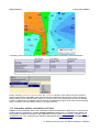
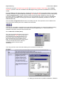
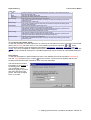
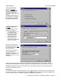
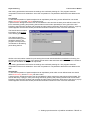
11 Setting up and execution of pathline calculations: TRACE ..... Chapter 11: Setting up and execution of pathline calculations: TRACE 11.1 Introduction......................................................................................................................................11-3 11.2 Pathline calulations in the TriShell ..................................................................................................11-3 11.2.1 Opening a pathline data set.....................................................................................................11-3 11.2.2 Allocating model parameters ..................................................................................................11-4 11.2.3 Start tracing from wells............................................................................................................11-4 11.2.4 User defined starting points.....................................................................................................11-5 11.2.5 Influence area (capture zone) calculation................................................................................11-5 11.2.6 Response curves.....................................................................................................................11-6 11.2.7 Executing pathline calculations................................................................................................11-6 11.3 Interactive pathline calculations in Triplot........................................................................................11-8 11.3.1 Menu bar in TriPlot (Trace)......................................................................................................11-9 11.3.2 How to trace within Triplot......................................................................................................11-10 11.4 Input data description.....................................................................................................................11-20 11.5 Output data description..................................................................................................................11-22 11.5.1 Binary output (*.bin)...............................................................................................................11-23 11.5.2 Printable summary (*.lst).......................................................................................................11-23 11.5.3 Execution log (*.log)...............................................................................................................11-23 11.5.4 Influence area result file (*.tro)...............................................................................................11-24 11.5.5 Response curve data (*.rsp)..................................................................................................11-24 11.5.6 Destination codes..................................................................................................................11-25 11.6 Mathematical background..............................................................................................................11-25 11.6.1 Introduction............................................................................................................................11-25 11.6.2 Calculation of the velocity field...............................................................................................11-25 11.6.3 Interpolation of local velocity..................................................................................................11-25 11.6.4 Particle tracking.....................................................................................................................11-27 11.6.5 Calculation starting from wells...............................................................................................11-27 11.6.6 Calculation from user defined points.....................................................................................11-28 11.6.7 Calculation of Influence Area.................................................................................................11-29 11.6.8 Technical Details and Error Messages..................................................................................11-31 Royal Haskoning Triwaco User's Manual 11.1 Introduction Once the groundwater flow situation has been calculated for a given hydrogeological situation, groundwater trajectories or flow lines may be computed using the particle-tracking program Trace. Apart from the calculation results (from the output file: flairs.flo) some additional information is needed. This information will be provided in the 'Path-line data set'. Currently there are two programs capable of calculating pathlines, Trace and Trawin. Trace is the default program used in Triwaco and for interactive pathline calculations in TriPlot. Trawin has some additional more advanced options. The different applications of the two will be described throughout the text. Additional options for more advanced pathline calculations cannot be entered directly from the TriShell. How to activate certain options is explained in the paragraph dealing with the input file. 11.2 Pathline calulations in the TriShell 11.2.1 Opening a pathline data set The 'Path-line data set' is created similarly to the other data sets by selecting 'Add' from the 'Dataset' pulldown menu and 'Path-lines' from the 'create new dataset' dialog window. The user is prompted to provide a description, the sub-directory name and the Calibration, Scenario or Transient data set the 'Path-line data set' is based on. This data set has to contain the groundwater flow simulation output file (flairs.flo). Confirming the selection with the OK-button causes the program to add the 'Path-line data set' to the 'project window'. Opening the 'Path-line data set window' displays the model parameters needed. Part of these parameters are adopted from the Calibration, Scenario or Transient data set referred to, other parameters have to be defined for the first time. Specific path-line parameters include the top and bottom elevations of all aquifers, the permeabilities/transmissivity of all aquifers and the effective porosity values for both aquifers and aquitards. The 'Path-line data set window' consists of three tab-sheets: Inherited parameters Modified parameters Result parameters This sheet displays those model parameters needed and defined in the data set the path-line data set is based on. This sheet displays all parameters created or modified in the (actual) path-line data set. This sheet may be used to display parameters that result from the trajectory calculations. Not all type of trajectory calculations result in parameters that can be displayed in the same way as input parameters and the groundwater flow result parameters. Pressing the right-hand mouse button displays the well-known pop-up menu, which enables the user to retrieve information, to view or edit the parameter's map or par file, and to examine the Ado file. The same actions may be achieved selecting the appropriate commands from the 'Parameter' pull-down menu. Selecting 'Modify parameter' moves the parameter from the Inherited parameters tab-sheet to the Modified parameters tab-sheet. The map and par files of the parameters moved to the Modified parameters tabsheet may be edited in the same way as the parameters from the 'Calibration data set'. Selecting 'Delete' from the 'Parameter' pull-down menu after having selected a parameter from the Modified parameters tab-sheet removes the parameter and restores the link to this parameter in the Inherited parameters tab-sheet. 11 Setting up and execution of pathline calculations: TRACE-3 Royal Haskoning Triwaco User's Manual 11.2.2 Allocating model parameters Similar to the allocation in the 'Calibration data set' selecting 'Allocate', from either the 'Parameter' pull-down menu or the pop-up menu, starts the selected allocator and an Ado file will be generated. After allocation the status of the parameter will change from to After successfully allocating parameter values for the path-line parameters one may start pathline calculations. Selecting 'Options' from the 'Path-lines' pull-down menu displays the 'Path-line options' dialog box. This dialog box contains three tab-sheets for the definition of different types of pathline calculations: Start tracing from Wells User defined starting points Influence area calculation This sheet displays the sources or wells for which pathline calculations have to be carried out. This sheet displays the file with user defined starting points for pathline calculations This sheet displays the options and the name of the grid file for influence area (capture zone) calculations. 11.2.3 Start tracing from wells The first tab-sheet, 'Start tracing from Wells', offers the possibility to define a number of path-lines starting in the vicinity of an infiltration or abstraction well. 11 Setting up and execution of pathline calculations: TRACE-4 Royal Haskoning Triwaco User's Manual The user has to provide the following information: • • • • • the source or well number for which path-lines are being computed, the number of radial points (e.g. the number of starting points lying on a circle with the selected well as it's center), the starting depth or elevation at which particle tracking starts, the angle between the line connecting the well and the first starting point and the positive x-direction and, finally, an end time, until which time particle trajectories are to be computed. Particle trajectories will be computed in upstream direction if the well is an abstraction well and in downstream direction for infiltration/injection wells. 11.2.4 User defined starting points The second tab-sheet, 'User defined starting points', offers the possibility to start particle trajectories at user specified points. These points are being defined by a common map and par-file, which have to be specified. The user has to provide the following information: • • • • the map-file (xyz.ung) defining the X and Y coordinates of the path-lines' starting points, the par-file (xyz.par) defining the elevation (or Z coordinate) of the path-lines' starting points, the tracing direction; e.g. Upstream or Downstream tracing or Both, and the end time, until which time particle trajectories are to be computed. 11.2.5 Influence area (capture zone) calculation The last tab-sheet, 'Influence area calculation', offers the possibility to compute the influence areas for wells, rivers and seepage areas. The path-line calculations start from a (large) number of points defined by a grid file, which is not necessarily the model's grid. A tool SYSAL is available for automatic identification of groundwater systems based in influence area calculation results. The user has to provide the following information: 11 Setting up and execution of pathline calculations: TRACE-5 Royal Haskoning • • Triwaco User's Manual the name of the grid file defining the path-lines' starting points, and the tracing direction; e.g. Upstream or Downstream tracing or Both ways. The end time is set by default to a value of 100,000 years (3652500 days). Note that, more options for influence area calculations are available when the calculation is carried out interactively in TriPlot. For instance definition of the starting depth. 11.2.6 Response curves The Influence area calculation set offers the user an additional option: 'Result as Response Curve' which allows the user to view the file containing the calculated response curves: Infl.rsp. A response curve, or hydrological response characteristic, is a curve that displays the distribution of travel times or residence times of the water, before it reaches a well, river or polder. The response curve is a cumulative frequency distribution, that is: the amount of groundwater with a residence time smaller than a given value is expressed as a percentage of the total discharge of groundwater. The results of the influence area calculation are also written to a file containing ado-sets. This file infl.tro may be loaded in TriPlot. The file contains the information about destination and the total residence time for each of the starting points. A detailed description is given with the destination codes (par. 10.5.6). 11.2.7 Executing pathline calculations Selecting 'Generate trace input file' from the 'Path-lines' pull-down menu will create four input files for the particle-tracking program Trace and Trawin. These files have default names well.tri for the path-lines starting at the wells, trace.tri for the user defined starting point, infl.tri for the computation of influence areas and inter.tri for interactive path line calculations in TriPlot. 11 Setting up and execution of pathline calculations: TRACE-6 Royal Haskoning Triwaco User's Manual Selecting 'Run predefined' from the 'Path-lines' pull-down menu the user can choose between the predefined calculation types. TriShell will start the particle-tracking program and calculate the path-lines defined in the input file of the corresponding set. The program will write the results of the path line calculations to a binary streamline file (*.bin) and to a printable list file (*.lst, Trace only). Information regarding the calculation process will be written to an execution log file (*.log). After termination of the computations, the results may be viewed graphically using TriPlot selecting 'Streamlines' from the pull-down menu. Similarly the print file and the execution log may be viewed selecting 'Result as Listing' or 'Log' from the pulldown menu. 11 Setting up and execution of pathline calculations: TRACE-7 Royal Haskoning Triwaco User's Manual A summary of the in and output files for the three predefined path line calculation sets is listed below: Input files Output files Binary streamline file Streamline listing Execution log Response curve Influence area output * Files generated by Trace only. Start tracing from Wells Wells.tri User defined starting points Trace.tri Influence area calculation Infl.tri Wells.bin Wells.lst * Wells.log - Trace.bin Trace.lst * Trace.log - Infl.bin Infl.lst * Infl.log Infl.rsp * Infl.tro Finally, selecting 'Interactive calculation' from the 'Path-lines' pull-down menu allows the user to start the graphical presentation tool TriPlot, load all parameter files needed and start particle-tracking interactively. Starting points may be defined in plane view or in a cross-section just by pointing the cursor to the desired location. In addition the groundwater velocity filed may be displayed through a vector field, the arrows being sized according to the groundwater velocity or having a fixed size. 11.3 Interactive pathline calculations in Triplot Triplot not only enables the user to view calculation results and streamlines in plane view or cross-sections, but also offers the possibility to calculate particle trajectories interactively. It is imperative that before one starts pathline calculations interactively with Triplot there should exist a Trace input file (*.tri) and a Trace configuration file (*.cfg). These files can easiest be generated in the Path-line data set of the Triwaco project. 11 Setting up and execution of pathline calculations: TRACE-8 Royal Haskoning Triwaco User's Manual Issuing the command 'Generate Trace input file' and 'Interactive calculation' 'Start Triplot' from TriShell's 'Path lines' pull-down menu the file inter.tri and inter.cfg are being generated and TriPlot is automatically started. Running TriPlot as stand-alone program, selecting the icon from the Triwaco Programs Folder, one can start interactive calculation of particle trajectories selecting 'File' from the 'Open' pull-down menu and subsequently a Trace configuration file (*.cfg file). This file contains all the information needed for tracing; e.g. grid information (location of grid.teo file), information on the groundwater flow system (location of the flairs.flo file) and specific information for tracing (top and base of aquifers and aquitards, porosities etc. from the Path-line data set). Once the Trace configuration file has been successfully read, the Trace pull-down menu is added to the menu bar and the following set icons is added to the the toolbar. The first icon is for pathline calculations from used defined starting points , the second for pathlines starting from wells and the third for creating a vector field all of which explained later on. These functions are availbale in both plane view and cross-sectional view. 11.3.1 Menu bar in TriPlot (Trace) The Trace Commands pull-down menu is being activated selecting 'Trace' from the menu bar. The pull-down menu has three sections. The first section offers the possibility to load and save streamline files and calculated vector fields. The second section allows various types of tracing and the third section offers the possibility to perform influence area calculations. The Trace pull-down menu offers the following sub-commands to choose from: Streamlines Load Save Clear Properties Loads an existing unformatted Trace output file with previously calculated streamlines. The program searches for files with extension *.bin. Saves the current streamline map to a Trace unformatted output file. Removes the (previously) calculated streamlines from the memory and clears the screen. Streamlines are not available any more, unless the streamline file has been saved, Displays the 'Streamlines Properties' window. This window provides some basic information regarding each streamline: number of points, total length, total residence time, first and last point's coordinates and the destination. The window is similar to the one used for selecting a streamline section. 11 Setting up and execution of pathline calculations: TRACE-9 Royal Haskoning Vector field Load Save Calculate Point tracing Well tracing Line tracing Area tracing Influence Area Triwaco User's Manual Loads an existing, previously calculated velocity vector map. The program searches for files with extension *.vec. Save the calculated velocity field. Calculate the velocity field for the current view. Start tracing from a point using the mouse-pointer. The user is prompted for the direction of tracing, the depth of the starting point and the total tracing time. Start tracing from a given well. The user is prompted for the ID of the well, the number and depth of the starting points and the total tracing time. Start tracing at equidistant points along a line. The user has to define the line using the mouse pointer. Subsequently the user is prompted for the distance between the points, the direction of tracing, the depth of the starting points and the total tracing time Start tracing at equidistant points within an area. The user has to define the area using the mouse pointer. Subsequently the user is prompted for the distance between the points, the direction of tracing, the depth of the starting points and the total tracing time Influence area or capture zone calculation. The user is prompted for the direction of tracing, the depth of the starting points and the total tracing time. 11.3.2 How to trace within Triplot To start the calculation of particle trajectories in Triplot one should select one of the commands in the second section of the 'Trace' pull-down menu or one of the following icons from the tool-bar: or . Triplot recognizes the following types of streamline calculations: point tracing, well tracing, line tracing and area tracing. The user is prompted for additional information and a specific pointer appears to define the point, line or area to start the particle tracking from. Calculated trajectories may be saved to an unformatted streamline file. Point tracing To start the computation of particle trajectories from a user defined point one should select 'Point tracing' from the 'Trace' pull-down menu or select from the tool-bar. A pop-up window appears and the user should provide the information needed for each of the four tab-sheets. The first tab-sheet contains information on the position of the starting point. The coordinates can be entered by typing or by 'point and shoot' with the mouse pointer, which has changed into a cross-mark. 11 Setting up and execution of pathline calculations: TRACE-10 Royal Haskoning Triwaco User's Manual The second tab-sheet defines the direction of tracing. One can choose between upstream tracing (backward in time) and downstream tracing (forward in time). The third possibility, both upand downstream, calculates the streamline that passes through the selected point. The third tab-sheet defines the depth of the starting point. The starting depth can be defined in three ways: 1. by a parameter (e.g. the groundwater table), 2. by an absolute depth (with respect to the reference level) or 3. by a relative position (with respect to the thickness of the selected aquifer or aquitard). The last tab-sheet defines the maximum residence time for the calculation of the particle trajectories. If the maximum residence time is exceeded the calculation is aborted and the destination code for the streamline is set to 0.7, "time exceeded". After having provided the information the settings are confirmed pressing Ok. The program starts the computation of the streamline. Once the computation is completed the streamline is added to the view. Repeatedly pointing the cursor to a new position and confirming the selection more streamlines will be calculated and added to the view. Well tracing To start the computation of particle trajectories from a given infiltration or abstraction well one should select 'Well tracing' from the 'Trace' pull-down menu or select from the tool-bar. A pop-up window appears and the user should provide the information needed for each of the four tab-sheets. 11 Setting up and execution of pathline calculations: TRACE-11 Royal Haskoning Triwaco User's Manual The first tab-sheet contains information on the position of the starting points. The position is defined by the source's ID, the number of points around the well and the number of vertical steps between the Top Depth and Bottom Depth (defined in the next two tabsheets). The second tab-sheet defines the Top Depth for the starting points. The top depth defines the highest elevation at which start points will be defined around the well. One can choose from the same options as with point tracing. The third tab-sheet defines the Bottom Depth for the starting points. The bottom depth defines the lowest elevation at which start points will be defined around the well. One can choose from the same options as with point tracing. The last tab-sheet defines the maximum residence time for the calculation of the particle trajectories. In the case of well tracing the direction of tracing depends on the type of well encountered. For an infiltration well the direction of tracing will be downstream (forward in time). Thus one can evaluate where the infiltrating groundwater is going. In case of an abstraction well the direction of tracing is upstream (backward in time) and one evaluates the origin of the abstracted water. 11 Setting up and execution of pathline calculations: TRACE-12 Royal Haskoning Triwaco User's Manual After having provided the information the settings are confirmed pressing Ok. The program starts the computation of the set of streamlines. Once the computation is completed the streamlines are added to the view. Line tracing To start the computation of particle trajectories at equidistant points along a user defined line one should select 'Line tracing' from the 'Trace' pull-down menu. A special cursor will appear and the user should define the line at which the start points will be located. The line is entered by pointing and pressing the left-hand mouse button repeatedly for every point of the line. Pointing to the last point's position and pressing the right-hand mouse button ends input of the line. A pop-up window appears and the user should provide the information needed for each of the four tab-sheets. The first tab-sheet contains information on the position of the starting points. The distance between successive starting points should be entered. The program will compute the coordinates for all starting points along the line. Similar to the information needed for point tracing the second tab-sheet defines the direction of tracing, the third tab-sheet defines the depth of the starting points and the last tab-sheet defines the maximum residence time for the calculation of the particle trajectories. After having provided the information the settings are confirmed pressing Ok. The program starts the computation of the set of streamlines. Once the computation is completed the streamlines are added to the view. Area tracing To start the computation of particle trajectories at equidistant points within a user defined area one should select 'Area tracing' from the 'Trace' pull-down menu. A special cursor will appear and the user should define the area at which the start points will be located. The area is defined by a polygon, each point being entered by pointing and pressing the left-hand mouse button. Pointing to the last point's position and pressing the right-hand mouse button ends input of the area. A pop-up window appears and the user should provide the information needed for each of the four tab-sheets. 11 Setting up and execution of pathline calculations: TRACE-13 Royal Haskoning Triwaco User's Manual The first tab-sheet contains information on the position of the starting points. The distance between successive starting points should be entered. The program will compute the coordinates for all starting points within the given area. Similar to the information needed for point tracing the second tab-sheet defines the direction of tracing, the third tab-sheet defines the depth of the starting points and the last tab-sheet defines the maximum residence time for the calculation of the particle trajectories. After having provided the information the settings are confirmed pressing Ok. The program starts the computation of the set of streamlines. Once the computation is completed the streamlines are added to the view. In case the combination of the area and the selected distance between the starting points results in a (very) large number of streamlines the program asks for confirmation. If confirmation is granted (pressing Yes) the computation of all streamlines is carried out. In case confirmation is denied (pressing No) the calculation of the streamlines is aborted. In that case the user should redefine the area and the distance between the starting points. How to calculate influence areas (capture zones) To start influence area calculations one should select 'Influence Area' from the 'Trace' pull-down menu. A pop-up window appears and the user should provide the information needed for each of the four tab-sheets. For influence area calculations the starting points should be located at the nodes of a valid Triwaco grid file. Apart from a standard streamline file the information on the influence area is written to a trace output file (*.tro). Furthermore, additional information for the computation of the response curves is written to a response file (with extension *.rsp). 11 Setting up and execution of pathline calculations: TRACE-14 Royal Haskoning Triwaco User's Manual The first tab-sheet contains information on the input and output files to be used. The name of a valid Triwaco grid file and the names of the trace output file and the response file have to be provided. Similar to the information needed for point tracing the second tab-sheet defines the direction of tracing, the third tab-sheet defines the depth of the starting points and the last tab-sheet defines the maximum residence time for the calculation of the particle trajectories. After having provided the information the settings are confirmed pressing Ok. The program starts the computation of the set of streamlines. Once the computation is completed the streamlines are added to the view. Whereas the 'Influence area calculation' option from the TriShell assumes all starting points are located at the top of the system, the calculation of an influence area with Triplot allows the user to specify the starting depth. Thus, one may discriminate between the influence area at the surface and at the top or the base of a confining layer. This distinction is important in defining groundwater protection areas around abstraction wells for the drinking water supply. How to calculate a velocity field Once a Trace configuration file (*.cfg) has been loaded into Triplot, groundwater velocities may be computed. The computed velocities may be displayed as a vector field or their values may be generated at the nodal points and treated as a regular Triwaco parameter. To start the computation of groundwater velocities one should select 'Vector Field' 'Calculate' from the 'Trace' pull-down menu or from the tool-bar. A pop-up window appears and the user should provide the information needed for each of the four tab-sheets. The first tab-sheet defines the type of velocity field to be calculated. The groundwater velocity can be computed at all nodes of the grid. This parameter (speed) can be treated as a regular Triwaco parameter and may be saved to an adore file. Moreover, groundwater velocity may be presented as a vector field map (vectormap). The vector filed may be saved to a specific file type (*.vec) for later use. 11 Setting up and execution of pathline calculations: TRACE-15 Royal Haskoning Triwaco User's Manual The second tab-sheet defines the depth the groundwater velocity is calculated for. The depth can be defined in three ways: 1. by a parameter (e.g. the elevation of a given layer), 2. by an absolute depth (with respect to the reference level) or 3. by a relative position (with respect to the thickness of the selected aquifer or aquitard). The third tab-sheet defines the position of the velocity vectors. The parameter speed is always computed at the grid's nodes. One can choose from calculation of the victors 1. at the centers of the elements, 2. at the location of all nodes and 3. equidistantly distributed over the model area at a user-specified distance. 11 Setting up and execution of pathline calculations: TRACE-16 Royal Haskoning Triwaco User's Manual The last tab-sheet defines the appearance of the arrows or vectors in the view. The velocity vectors may be represented by arrows of fixed dimensions or the size of the vectors may vary with the calculated velocity according to a scaling factor. The scaling factor is defined in terms of the distance traveled during a user-specified time. The calculated groundwater velocity parameter (speed) may be saved selecting 'Save' from the 'Param' pulldown menu. The calculated vector filed may be saved selecting 'Vector field' 'Save' from the 'Param' pulldown menu. The program prompts to select the parameter or vector field to be saved and to define a file name. After confirmation the parameter or vector field is available for later use. Tracing in a cross-section Similar to the calculation of streamlines and a vector field in plane view one can start these calculations from a cross-section. Obviously not all options are available. 11 Setting up and execution of pathline calculations: TRACE-17 Royal Haskoning Streamlines Vector field Calculate Velocity Map Triwaco User's Manual The Streamlines sub-commands are disabled Calculate the velocity field for the current cross-section. The user is prompted for the distance between the vectors. Both the horizontal and vertical vector spacing should be given. Calculates the velocity field for the current cross-section to be presented by contours or classes. The user is prompted to define the average (horizontal) node-distance to be used for the contour-plot. After having supplied this information, the program generates a triangular grid, computes the groundwater velocity at all nodes and starts contouring the parameter 'Velocity'. 11 Setting up and execution of pathline calculations: TRACE-18 Royal Haskoning Point tracing Triwaco User's Manual Start tracing from a point using the mouse-pointer. The coordinates can be entered by typing or by 'point and shoot' with the mouse pointer, which has changed into a cross-mark. The user has to define the direction of tracing and the total tracing time. To start the computation of a vector field of groundwater velocities in the cross-section one should select 'Vector Field' 'Calculate' from the 'Trace' pull-down menu or from the tool-bar. A pop-up window appears and the user should provide the information needed. Only two tab-sheets are available. The computation of a velocity parameter for contouring can not be initiated from this window. The magnitude of the groundwater velocity may be calculated issuing the commands 'Vector Field' 'Velocity map' from the 'Trace' pull-down menu. To start the computation of particle trajectories from a user defined point in a cross-section one should select 'Point tracing' from the 'Trace' pull-down menu or select from the tool-bar. A pop-up window appears and the user should provide the information needed for each of three tab-sheets. Coordinates are needed for X, Y and Z-direction and can be entered by 'pointing and shooting' with the mouse pointer. 11 Setting up and execution of pathline calculations: TRACE-19 Royal Haskoning Triwaco User's Manual While generating particle trajectories in a cross-section the calculated trajectories will also be displayed in plane view. Loading, saving or clearing of calculated particle trajectories is only possible in plane view. These options are disabled in the 'Trace' pull-down menu. 11.4 Input data description The program Trace requires three main data input files, and a (large) number of complementary data files for definition of the hydrogeological parameters. The first input file is the grid file grid.teo, generated by on of the grid generators. This file contains all information about the grid structure. The second data input file (flairs.flo) contains the results of the groundwater flow computations. The third data input file (*.tri) contains the definition of the trace system and of the starting points. This input file will be different for the three types of flow line calculations. The input files will be generated by the TriShell issuing the command 'Generate trace input file' from the 'Path lines' pull down menu, after having entered the information needed in the Pathline Options window. Set 1: HEAD Format A40 · identification of pathline calculation HEAD is an alphanumerical string for identification of the pathline calculation Set 2: consists of three records FO FLOname FLOtype FO FLOname FLOtype · Definition of flow system · File name of flow system · Type of simulation result Definition of the flow system The name of the file containing the flow system (usually flairs.flo), including the relative path Type of simulation result of the flow system (Steady state calculation or Transient calculation) Set 3: consists of three records FI FLIname FLItype FI FLIname FLItype · Definition of flow system · File name of flow system · Type of simulation result Format A2 Format A60 Format A20 Definition of the flow system (input file) The name of the file containing the input of the flow system (usually flairs.fli), including the relative path Type of simulation result of the flow system (Steady state calculation or Transient calculation) Set 4: consists of three records IPname IFname IFPname IPname IFname IFPname Format A2 Format A60 Format A20 · Triwaco inherited parameter name · parameter file name · user defined parameter name Format A4 Format A60 Format A20 is the pre-defined inherited Triwaco parameter name the name of the file containing the parameter, including the relative path a user defined name describing the parameter; this name may be different from the predefined parameter name. Set 4 should be repeated as many times as required. If Pname is not one of the pre-defined Triwaco parameter names necessery for pathline calculations, Set 4 will be ignored. Parameters that are not defined by Set 4 will obtain a default value equal to 0, except for the anisotropy parameters PYi and TYi, which will be assigned the value of the corresponding PXi and Txi. Set 5: consists of three records PPname PFname PFPname PPname · Triwaco pathline parameter name · parameter file name · user defined parameter name Format A4 Format A60 Format A20 is the pre-defined Triwaco pathline parameter name 11 Setting up and execution of pathline calculations: TRACE-20 Royal Haskoning PFname PFPname Triwaco User's Manual the name of the file containing the parameter (including the relative path) a user defined name describing the parameter; this name may be different from the predefined parameter name. Set 5 should be repeated as many times as required. If Pname is not one of the pre-defined Triwaco parameter names necessery for pathline calculations, Set 5 will be ignored. Parameters that are not defined by Set 5 will obtain a default value equal to 0. Set 6: End · literal text string This string should always be present, it indicates the end of the section Set 7a:user defined starting points N Nx, Ny, Nz, Nd N Nx,Ny,Nz Nd · Type of calculation (N>0), number of points · X, Y, Z coordinate and direction Number of user defined starting points (Npnt >0), if Npnt=0 records specifying starting points are skipped. X-, Y-, Z- co-ordinate of the starting point Direction of pathline calulation (-1 is upstream, 1 is downstream, 2 is upstream and downstream) Set 7b:influence area calculation N, Nd, Nname N Nd Nname · Type of calculation (N=-1), direction, grid file name Format ?? Influence area calulation (Npnt =-1), if Npnt=0 record specifying influence area calculations is skipped. Direction of pathline calulation (-1 is upstream, 1 is downstream, 2 is upstream and downstream) The name of the grid file containing the starting points (including the path) Set 8:start tracing from wells W Wid, Wn, Wz, Wa W Wid Wn Wz Wa Format A4 Format ?? · Triwaco parameter name · Well ID, Number of pathlines, Starting depth, Angle Format A4 Format ?? Number of user wells (W >0), if Npnt=0 records specifying wells are skipped. ID of the well as specified in the grid The number of particles that should be started around the well The depth or Z-coordinate of the starting points The angle with the positive X-direction for the determination of the first starting point's location The direction of tracing depends on the type of well. For abstracting wells the direction of tracing is upstream, for infiltrating wells the direction is downstream. Set 9: Definition of maximum residence time NTIM T(1), T(2), ..., T(NTIM) T(n) · number of time steps to be marked on the pathlines (NTIM>0) · time of travelling of the traced water particle to be marked on the pathline T(n+1)>T(n) Format FREE Format FREE The last section of the input file defines the duration of the particle tracking calculations and the definition of (intermediate) print output times. The first record defines the number of times (relative to the start time) that should be read. The next records contain the residence times in increasing order. The last time defines the maximum residence time for the calculation. If this time is exceeded the calculation is stopped and the appropriate destination code (0.7) is assigned to the trajectory. Usually only one time (the end time) is specified. 11 Setting up and execution of pathline calculations: TRACE-21 Royal Haskoning Triwaco User's Manual Example of input file (*.tri) SET 1 2 3 4 4 5 5 5 5 5 5 6 7a 7b 8 9 Example Text New Trace Data set FO ..\NewRef\flairs.flo Steady state calculation FI ..\NewRef\flairs.fli Steady state calculation TX2 ..\NewRef\TX2.ado TX2 TX3 ..\NewRef\TX3.ado TX3 … TT TT.ado TT RL2 RL2.ado RL2 TH6 TH6.ado TH6 PC0 PC0.ado PC0 PA1 PA1.ado PA1 PC5 PC5.ado PC5 end ... 2 161450.000 380810.000 -10.000 2 161400.000 380690.000 -10.000 2 -1 -1 ..\NewGrid\grid.teo 2 109 8 -25 0 109 8 -65 0 2 365, 18262 Description Heading Definition of flow system Relative path and file name Optional, Definition of input file Only required for Variable Density calculations. Definition Inherited parameter Relative path and file name Name of adore-set Definition Inherited parameter Definition Path line parameter (top topsystem) Relative path and file name Name of adore-set Definition Path line parameter Relative path and file name Name of adore-set Definition Path line parameter Relative path and file name Name of adore-set Definition Path line parameter (porosity topsystem) Relative path and file name Name of adore-set Definition Path line parameter (porosity aquifer 1) Relative path and file name Name of adore-set Definition Path line parameter (porosity aquitard 5) Relative path and file name Name of adore-set End of parameter section Number of Starting Points X-, Y- and Z-coordinates, direction of tracing. Definition starting points, direction of tracing, relative path and file name of grid Number of Wells Well ID, number of startpoints, z-coordinate and angle Well ID, number of startpoints, z-coordinate and angle Number of output times Output times 11.5 Output data description The calculation results are written to three general output files. For influence area calculations two additional output files are generated. The general output files are the *.bin file, containing binary output of the calculated particle trajectories, the *.lst file, containing a printable summary of the calculated particle trajectories and the execution log file *.log. The first of the additional output files for influence area calculations is the file Infl.tro, containing destination codes, residence times and trajectory lengths in adore format. The second is the file Infl.rsp, containing the information for the generation of the response curves. A summary of the output files is given below: File type Well tracing User defined points Binary output well.bin trace.bin Printable summary well.lst trace.lst Execution log well.log trace.log Influence area data N/A N/A Response curve data N/A N/A * For interactive calculations the filenames are user defined. Influence area infl.bin infl.lst infl.log infl.tro infl.rsp Interactive* inter.bin inter.lst inter.log inter.tro inter.rsp 11 Setting up and execution of pathline calculations: TRACE-22 Royal Haskoning Triwaco User's Manual 11.5.1 Binary output (*.bin) The binary output files can be viewed only using the graphical presentation tool TriPlot. After opening the grid file the binary output can be loaded selecting 'Streamline map' from the 'View' pull-down menu or from the Pathlines pull down menu in the TriShell-Pathline data set. The particle trajectories can be viewed in plane view or in a vertical cross-section. A distinction between particle trajectories is possible for different destinations or along one and the same trajectory for increasing residence time. 11.5.2 Printable summary (*.lst) The printable summary contains for all successive trajectories the complete path line information. This information consists of a serial number (of the successive points on the trajectory), the residence time (in days), the X-, Y- and Z-coordinates, a code for the aquifer or aquitard the trajectory crosses and the destination code. The destination code remains 0 as long as the calculation continues. Only for the last point of the trajectory the destination code is written to file. The code for the aquifer or aquitard consists of the serial number of the layer with positive values referring to an aquifer and negative values referring to the aquitards. 1 0 161003 380529 -50 2 0 2 5.8495 161004 380529 -49.982 2 0 ……… 177 17246.5 160784 376779 0.234686 2 0 178 17349.2 160781 376760 0.670974 -1 0 179 18262 160781 376760 4.17216 1 0.7 1 0 161002 380531 -50 2 0 2 5.70922 161003 380531 -49.9842 2 0 11.5.3 Execution log (*.log) The execution log file contains information on the calculation process and a summary of the computed particle trajectories. This information consists of: A list of the total path and file names of the Trace-input and output files that have been used. A list of all hydrogeological parameters that have been loaded, followed by a summary of parameter values. A check of the Trace-system. The corrections that are performed by the program to obtain a valid Trace-system are reported. If the system is not valid Error-messages will be printed. A summary of distinctive points for each path line. This summary contains the trace-step number, the X-, Y- and Z-coordinate of the point reached, the total travel time and the travel time between successive points and a description of the layer or destination reached (shown below). Start of run: Mon Apr 02 14:49:57 2001 257 starting points. Streamline 1. 1 161620.00 380580.00 93 161392.09 380660.18 …… Streamline 10. 1 160710.00 380220.00 12 160776.44 380305.89 13 160776.44 380305.89 38 160847.91 380349.83 …… End of run: Mon Apr 02 14:50:04 2001 -41.25 -42.21 start 243.31 days 0.00 244.37 Aquifer 2 Source 108 13.90 -3.43 -9.38 -10.21 start 7.10 years 9.46 years 9.72 years 0.00 109.99 115.95 200.26 Aquifer 1 Aquitard 1 Aquifer 2 Source 148 In case an Error in the Trace-system occurs no path lines will be computed. The user should consult the execution log file in order to establish which parameter caused the error. Possible causes are the omission of a parameter that is needed (because the parameter has not been allocated yet) or the existence of a 0-value for the transmissivity or permeability of one of the aquifers. 11 Setting up and execution of pathline calculations: TRACE-23 Royal Haskoning Triwaco User's Manual For influence area calculations the execution log file also contains information on the total discharge for each source and each river. This information is used for the calculation of the response curves. Response curve calculation with 2717 starting points. Sum of discharges in m3/d: River 63 (#63): 11669.16+0.00+0.00+0.00+0.00+0.00=11669.16 …… Source 63 (#51): 0.00+0.00+0.00+3204.00+0.00+0.00=3204.00 11.5.4 Influence area result file (*.tro) The first of the additional output files for influence area calculations is the file Infl.tro. This file contains the following parameter sets in adore format: X-STARTPNTS Y-STARTPNTS Z-STARTPNTS TIME LENGTH DESTINATION X-DESTINATION Y-DESTINATION Z-DESTINATION Q-RECHARGE Q-RIVER NODE INFLUENCE AREA= X-coordinate of the starting points. This set is copied from the grid-file used for the influence area calculations. Y-coordinate of the starting points. This set is copied from the grid-file used for the influence area calculations. Z-coordinate of the starting points. This set is equal to the phreatic surface, set PHIT from the groundwater flow output file (flairs.flo). The calculated total residence time of the path line. The calculated total length of the path line. Destination code; description of the end point of the calculated path line X-coordinate of the end point of the calculated path line. Y-coordinate of the end point of the calculated path line. Z-coordinate of the end point of the calculated path line. Vertical flux at upper boundary. This set is equal to the set QRCH from the groundwater flow output file (flairs.flo). River flux calculated from the corresponding parameters in the groundwater flow output file (flairs.flo). The value is set to 0 for nodes that do not belong to a river. Influence area of the starting point's node. This set is copied from the grid-file used for the influence area calculations. 11.5.5 Response curve data (*.rsp) The second additional output file for influence area calculations is the response curve file Infl.rsp. This space delimited output file contains the data to generate the response curves: the Destination code, the residence Time of the Volume that reaches the source or river and the cumulative proportional volume for that time (Volume%) Thus, for each source and river, the response curve expresses the amount of groundwater that has reached the destination with a residence time smaller than a given value as a percentage of the total discharge of groundwater for that destination. "Dest" "Time" "Volume" "Volume%" 1 0 1.14745 0.0458981 1 5.57416 1.08886 0.0894525 1 5.61345 1.08965 0.133039 ... 1 25250.5 22.4573 92.5484 1 27742.6 18.8667 93.303 11 Setting up and execution of pathline calculations: TRACE-24 Royal Haskoning Triwaco User's Manual 11.5.6 Destination codes The destination code in the influence area output file (infl.tro) defines the character of the location of the end point of the flow line. A negative integer indicates that the flow line ends in a river, with the absolute value of the number being the river number or river ID assigned to that river. A positive integer indicates that the flow line ends in a well, with the number being the source number or source ID assigned to that well. Other destinations are indicated by a destination code with values between -1 and +1. The next table summarizes the destination codes generated by the particle-tracking program Trace: Destination code -1 -0.5 -0.4 -0.3 0.1 - 0.3 0.5 0.7 1 Description of destination negative integer: number of river reached (c.f. grid.teo) flow line leaving the system vertically (top-system reached) flow line immediately leaving the system vertically: upstream tracing in area with downward seepage (infiltration) flow line immediately leaving the system vertically: downstream tracing in area with upward seepage (e.g. a polder) stagnant points reached flow line leaving the system horizontally (crossing the model boundary) maximum tracing time reached (time specified in the input file) positive integer: number of source reached (c.f. grid.teo) 11.6 Mathematical background 11.6.1 Introduction Trace determines pathlines and travel times in groundwater flow, based on groundwater flow simulations (flairs.flo). The pathlines are determined in three dimensions. The horizontal movement is derived from the discharges that have been calculated for the aquifers. The thickness and the porosity of the aquifer are used to calculate the velocity corresponding to the discharge. The vertical movement within the aquifers is derived from vertical fluxes through the aquitards, using the principle of continuity (so that the vertical flux varies linearly between the flux on the top of the aquifer and the flux at the bottom). Vertical movement is been taken into account for the slope of the aquifer. The vertical movement depends on the slope of the top of the aquifer and the slope of the bottom. The transport through the aquitards is vertical only. Together with the porosity and thickness of the aquitard, the time needed for the passage through the aquitard is calculated. The pathlines can be determined following the flow upstream and downstream. In calculating the flow lines (or particle trajectories) the program uses a large number of successive small steps through the elements of the grid. The length of these steps depends on the size of the elements and on the velocity of the groundwater. Travel times passed since the start of the tracing are computed and may be indicated on the flow lines using time markers. For each time step both a horizontal and a vertical velocity and displacement is calculated. 11.6.2 Calculation of the velocity field Before tracing starts, the velocity field in every aquifer is calculated. First the velocity components at the centers of the elements are determined applying Darcy’s law locally for the element concerned. In this element the normal to the plane describing the groundwater head in the aquifer is computed. Subsequently this vector is projected on the horizontal plane resulting in a 2D gradient vector. Next, the quotient of the permeability tensor and the effective porosity at the three corner points (grid nodes) of the element is averaged. The gradient vector is scaled by this average, resulting in a horizontal effective velocity at the element center. Finally, the horizontal velocity at every grid node is calculated as the average of the velocities at all surrounding elements. This double averaging method results in a smooth, continuous velocity field. 11.6.3 Interpolation of local velocity During the tracing of a water particle, its 3D-velocity vector needs to be calculated at any point in the model’s domain. Prior to the calculation of the velocity the number of the element and the layer in which the particle is located have to de determined. Moreover the value of the linear shape function in the element considered should be known. These shape functions ( ) are used for the interpolation within the element: 11 Setting up and execution of pathline calculations: TRACE-25 Royal Haskoning Triwaco User's Manual with: the interpolated value of the parameter z at location x the shape function value for vertex i of the element considered the value of parameter z at vertex i of the element considered Aquifer velocity The horizontal velocity vector velocity field in the aquifer at point p is interpolated using the pre-calculated horizontal . The vertical velocity component is computed from the local vertical fluxes through the adjoining aquitards. After linear interpolation between the fluxes at the top and those at the base of the aquifer, division by the aquifer’s effective porosity at point p and adjustment for the slope of the aquifer, the vertical velocity component becomes: with: The vertical velocity component at point p The (vertical) flux through the overlying aquitard at point p The (vertical) flux through the underlying aquitard at point p The normalized distance to the top of the aquifer at point p The normalized distance to the base of the aquifer at point p The effective porosity of the aquifer at point p The gradient of the top plane of the aquifer at point p The gradient of the bottom plane of the aquifer at point p Aquitard and top system velocity In aquitards only vertical flow is assumed. At the particle’s location the vertical flux through the aquitard and the effective porosity are computed using weighted linear interpolation with shape functions. The vertical velocity is calculated as: with: the vertical velocity at point p the (vertical) flux at point p, through the aquitard considered the effective porosity of the aquitard at point p 11 Setting up and execution of pathline calculations: TRACE-26 Royal Haskoning Triwaco User's Manual 11.6.4 Particle tracking The particle-tracking program will evaluate the particle’s starting point prior to the computation of its trajectory. If the particle's starting point passes the initial checks its trajectory will be evaluated. During the tracing procedure the location at every step is recorded and the program checks whether or not the stopping criteria are met. As soon as one of these criteria is met computation of the particle’s trajectory is ended. The particle’s trajectory is evaluated in upstream or downstream direction, as a series of movements consistent with the local groundwater velocity calculated. After each displacement the actual location of the particle and the time passed since the beginning of the trajectory calculation are recorded. The calculation is repeated for each starting point specified. If a particle reaches a draining river, either from below or from the sides, particle tracking will be aborted. The last point of the particle’s trajectory will be the intersection point of the trajectory and the river's bank or bottom. A particle reaches a river from the side when it crosses the riverbank. Riverbank coordinates are calculated using the river widths (RWx) supplied in the river input file. 11.6.5 Calculation starting from wells Particle tracking can be started on a user-specified number of starting points around one or more selected wells, the sources. The well number, the number of starting points around the well and the depth of the starting points have to be specified in the corresponding tab-sheet of the Path line Options window. This information is read by the TriShell and copied to the Trace input file (Well.tri). The starting points will be distributed on a circle with the well as its center. In case of establishing particle trajectories in upstream direction starting at an abstraction well, the starting point is chosen at a distance of approximately one half of the bisector of the first element encountered. At smaller distances the computed velocity field will not be accurate, nor will the particle's trajectory. As a consequence the starting time at the starting point will not be equal to 0; it is computed analytically using 11 Setting up and execution of pathline calculations: TRACE-27 Royal Haskoning Triwaco User's Manual the following equation: with: the thickness of the aquifer at the location of the well the distance between the well and the starting point the effective porosity of the aquifer considered the discharge of the well Note that this is a rough approximation because neither the velocity field around the well nor the variations in aquifer thickness or porosity are taken into account. Similarly, a water particle is supposed to have reached an abstraction well whenever the distance to the well is smaller than the radius of the node influence area of that well. The equation mentioned above is used to calculate the final destination time. The exact location of the starting points is calculated by the program. From these starting points the particle trajectories are computed, in upstream direction for an abstraction well and in downstream direction for infiltrating wells. The calculation results are written to three output files: the file well.bin, containing binary output of the calculated particle trajectories, the file well.lst, containing a printable summary of the calculated particle trajectories and the execution log file well.log. 11.6.6 Calculation from user defined points Particle tracking also can be started on a number of user-specified starting points. These points are defined through an ordinary map and par file. The files, defining the starting points, have to be specified in the corresponding tab-sheet of the Path line Options window. This information is read by the TriShell and copied to the Trace input file (Trace.tri). In addition the user should specify the direction of tracing: upstream, downstream or both. 11 Setting up and execution of pathline calculations: TRACE-28 Royal Haskoning Triwaco User's Manual From these starting points the particle trajectories are computed, in the direction specified by the user. The calculation results are written to three output files: the file trace.bin, containing binary output of the calculated particle trajectories, the file trace.lst, containing a printable summary of the calculated particle trajectories and the execution log file trace.log. The binary output can be viewed with Triplot. 11.6.7 Calculation of Influence Area Finally particle tracking can be started at each node of a grid. This grid is not necessarily the same as the model grid used for groundwater flow calculations. The only restriction for the grid is that the area is within the boundaries of the model grid. Thus a strongly refined grid, covering part of the model's domain can be used for the influence area calculations. In that case the results should be presented for this refined grid. The grid to be used for the calculations should be specified in the corresponding tab-sheet of the Path line Options window. This information is read by the TriShell and copied to the Trace input file (Infl.tri). In addition the user should specify the direction of tracing: upstream, downstream or both. Generally influence area calculations are carried out in downstream direction, to detect the destination of particle trajectories starting in a given area. From the starting points (the grid's nodal points) the particle trajectories are computed, in the direction specified by the user. The calculation results are written to the three standard output files: the file infl.bin, containing binary output of the calculated particle trajectories, the file infl.lst, containing a printable summary of the calculated particle trajectories and the execution log file infl.log. Additional information is written to the influence area output file infl.tro and to the response curve output file infl.rsp. 11 Setting up and execution of pathline calculations: TRACE-29 Royal Haskoning Triwaco User's Manual The calculation of an influence area enables the user to compute a great number of flow lines starting in a given area. This area can be a (small) part of the model area or the complete model area. Starting points in the area may be defined in a separate grid or in the model’s grid nodes. The influence area results file (infl.tro) contains the coordinates of the start and end points for each flow line, the total length of the particle's trajectory and the total residence time of the groundwater, the recharge (or discharge) at the starting point, the node influence area for the starting points and a destination code. These data are given in the output file in separate adore-sets, in concordance to the size of the grid specified. The destination code in the influence area output file (infl.tro) defines the character of the location of the end point of the flow line. A negative integer indicates that the flow line ends in a river, with the absolute value of the number being the river number or river ID assigned to that river. A positive integer indicates that the flow line ends in a well, with the number being the source number or source ID assigned to that well. Other destinations are indicated by a destination code with values between -1 and +1. The next table summarizes the destination codes generated by the particle-tracking program Trace: Destination code -1 -0.5 -0.4 -0.3 0.1 - 0.3 0.5 0.7 1 Description of destination negative integer: number of river reached (c.f. grid.teo) flow line leaving the system vertically (top-system reached) flow line immediately leaving the system vertically: upstream tracing in area with downward seepage (infiltration) flow line immediately leaving the system vertically: downstream tracing in area with upward seepage (e.g. a polder) stagnant points reached flow line leaving the system horizontally (crossing the model boundary) maximum tracing time reached (time specified in the input file) positive integer: number of source reached (c.f. grid.teo) For all nodes of the grid specified particle trajectories are being computed. The trajectories all start by default at the top of the hydrogeological system (defined by the parameter TT). The tracing will be carried out in the direction specified by the user. Upstream tracing will follow the particle’s trajectory backward in time, whereas downstream tracing follows the flow line forward in time. For influence area calculations of an arbitrary area (not a grid) the user should define the area in the Interactive Calculation mode. Also if the user wants the calculation of an influence area starting at an arbitrary depth (not equal to TT) the calculation should be carried out in the Interactive Calculation mode. Interactive Calculation of particle trajectories is possible selecting 'Interactive calculation' 'Start TriPlot' from the 'Path lines' pull-down menu or by opening the file 'Inter.cfg' in Triplot. 11 Setting up and execution of pathline calculations: TRACE-30 Royal Haskoning Triwaco User's Manual 11.6.8 Technical Details and Error Messages Prior to and during the particle trajectory calculation the particle's location is submitted to a number of checks. Moreover, before starting the tracing routine the whole hydrogeological system is verified. Whereas the groundwater flow calculation program (i.e. Flairs) accepts 0-values for the transmissivity, the permeability and the hydraulic resistance of the separating layers the path line program Trace does not accept 0-values at all. Therefore, the program checks whether or not a 0-value exists either for the transmissivity or permeability or for the thickness of the aquifers and aquitards. If a 0-thickness for one of these layers is encountered the program corrects the corresponding values of top or base of the aquifer such that a minimum thickness of 0.10 m is guaranteed. If the program encounters a 0-value for the transmissivity or permeability it generates an error message stating there is an "error in the tracing system" and subsequently terminates the calculation process. Initial checks Before a particle is submitted to the tracing routine, it’s location in the model is evaluated. In the following cases no particle trajectory is computed: The starting point lies beyond the model’s boundary or below the base of the lowermost aquifer. The starting point belongs to a draining river and particle tracking is downstream. Similarly, for upstream particle tracking the starting point should not belong to an infiltrating river. The starting point is located at an abstraction well and particle tracking is downstream. Similarly, for upstream particle tracking the starting point should not be located at an infiltrating well. The starting point is located at the water table in an area where seepage takes place and particle tracking is downstream. Similarly, for upstream particle tracking the staring point should not be at an infiltration area. Although actually no particle trajectory is being calculated the start and end points (being exactly the same) are written to the output files and in case of influence area calculations the proper destination code is assigned to the trajectory. The length of such a trajectory is by definition equal to 0. In the following cases the particle’s starting location is adjusted: The particle’s starting point is situated above the water table. The z-coordinate of the starting point is adjusted to that of the water table at the particle’s starting location. The particle’s starting point is located at an infiltrating river. The z-coordinate of the starting point is adjusted to that of the bottom of the river at the particle’s starting location. The particle's trajectory is calculated from the adjusted starting point. The total residence time of the particle is not adjusted, even if one might expect a slightly higher residence time due to percolation through the unsaturated zone. Stopping criteria Once the starting location of a particle has been determined its course through the groundwater flow system is followed until one of the following stopping criteria is met: The end time has been reached; this time has to be specified in the input file. The particle reaches a stagnant zone. In a stagnant zone the groundwater flow velocity drops below a threshold value of 1 mm/yr. The particle exits the system; the particle has reached the model’s boundaries, an abstraction well, a draining river or a seepage area of the top-system. The calculation of the next point on a flow line is achieved by integration, using a second order Runge Kutta method. The integration step size depends on the element size and is taken as: In this equation 'A' stands for the area of the element in which the particle is located. Using this integration step the particle's trajectory is evaluated with an average of 20 steps per element. 11 Setting up and execution of pathline calculations: TRACE-31 Royal Haskoning Triwaco User's Manual If a particle crosses an inter-layer boundary while moving to the next location, the intersection point of the flow line with the layer boundary is taken as the next point. The following relation evaluates the time needed to travel to the next location: with: the increase in travel time the particle’s present location the particle’s next location the groundwater flow velocity at the particle’s present location the groundwater flow velocity at the particle’s next location 11 Setting up and execution of pathline calculations: TRACE-32