Download EFDC_Explorer 7.3 Guidance New Features and

EFDC_Explorer 7.3 Guidance
New Features and Functionality
Release:
28 May 2015
Table of Contents
1
2
Major New Features of EE7.3 .................................................................................. 3
Ice Sub-Model .......................................................................................................... 4
2.1
Use External Ice Time Series (ISICE = 1) ......................................................... 5
2.2
Use Specified ON/OFF Ice Cover (ISICE = 2) ................................................... 6
2.3
Use Heat Coupled Ice Model (ISICE = 3) .......................................................... 7
2.4
Frazil Ice Transport (ISICE = 4) ........................................................................ 8
2.5
Visualization of Ice ............................................................................................ 8
3 Evaporation and Forced Evaporation Tool ............................................................. 12
Forced Evaporation Methodology .......................................................................... 17
4 NetCDF Output ...................................................................................................... 20
4.1
Displaying NetCDF data in ArcGIS ................................................................. 22
4.1.1. Visualizing NetCDF data .......................................................................... 22
5 Waves Functionality Updates ................................................................................. 28
5.1
Waves Tab ..................................................................................................... 28
5.1.1. Wave Models in EFDC ............................................................................. 28
5.1.2. Internal Wave Model Option..................................................................... 29
5.1.3. External Wave Model Option ................................................................... 30
5.1.4. Creating SWAN Model Output – Running SWAN from EE ....................... 33
5.1.5. Use SWAN Model Output ........................................................................ 36
6 Flight Path Animation ............................................................................................. 37
7 Automated Atmospheric and Wind Series Weighting ............................................. 41
8 Elimination of Template Files ................................................................................. 45
9 Miscellaneous Updates .......................................................................................... 47
9.1
Export Toxics in Tecplot Update ..................................................................... 47
9.2
3D Symbols .................................................................................................... 48
9.3
Buffer loading for EE drifters ........................................................................... 49
9.4
Subscript and Superscript in Graph Legends .................................................. 49
9.5
Delete Lines from Line Options (Time Series Grapher) ................................... 50
9.6
Display Miles or Feet in Labels ....................................................................... 52
9.7
Specify Color Ramps ...................................................................................... 53
9.8
Particles on the boundary disappear in 3D ...................................................... 55
9.9
Change Legend Font Sizes............................................................................. 57
9.10 Display Wind and Atmospheric Stations in ViewPlan ...................................... 58
9.11 WSER, TSER and ISER Timeblocks .............................................................. 60
9.12 Automatic Seat Deactivation ........................................................................... 63
9.13 Date and Coordinate Conversion Tool ............................................................ 64
9.14 Display Model Comparisons in Time Series .................................................... 65
10 Appendix Data Formats ......................................................................................... 68
11 References ............................................................................................................ 73
www.efdc-explorer.com
2
May 2015
1 Major New Features of EE7.3
Dynamic Solutions – International, LLC continues to strive to further develop the functions
and capabilities of the EFDC_DSI/EFDC_Explorer Modeling System. This latest release of
EE provides many notable new features as well as numerous minor bug fixes and tweaks.
EE undergoes rigorous testing to ensure accuracy of results. New major features of EE7.3
include the following:

Ice Sub-model

Forced Evaporation

NetCDF Output

Run SWAN from within EE

Elimination of Template Files

Flight Path Animations
www.efdc-explorer.com
3
June 2015
2 Ice Sub-Model
EFDC_Explorer7.3 now implements a robust ice sub-model. Previously EFDC had relatively
limited ice modeling ability. In EE7.2 and earlier the ice conditions had to be fully specified
by the user for every cell for the model simulation period. The creation of the input files was
also external to EE. Now ice formation and melt is simulated by EFDC using a coupled heat
model and fully handled by EFDC_Explorer.
Note that ice dynamics are not modeled at this stage. An ice dynamics sub-model would
simulate the constriction of the channel by ice and the resulting bed shear caused by the
transport of ice chunks. An ice dynamics sub-model is being considered for a later release of
the EE modeling system.
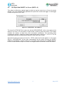
Ice options are now available under a new Ice Options sub tab under the Temperature tab
as shown in Figure 2-1. For all the options, ice is only enabled if the user is simulating
temperature.
Figure 2-1 Temperature Tab: Ice Sub Model Options.
www.efdc-explorer.com
4
May 2015
Options for the ice sub model include:
ISICE = 0
ISICE = 1
ISICE = 2
ISICE = 3
ISICE = 4
Do not use ice
Use External Ice Time Series (ISER & ICEMAP)
Use Specified ON/OFF Ice Cover (ISTAT)
Use Heat Coupled Ice Model
Use Heat Coupled Ice Model with Frazil Transport
Application and operation of each of these options is explained in the following sections.
2.1
Use External Ice Time Series (ISICE = 1)
This option is similar to the ice option available prior to EE7.3 and does not compute ice
formation/melt and it is not linked to the heat balance. This option simply requires the user
to provide a fraction of ice coverage and thickness of ice for every cell using formats
provided in Appendix B-16 and B-17. The primary impact of the ISICE =1 option is on
processes that occur at the air/water interface and has no direct impact on ice melt. For
those cells where ice is present the ice sub-model will:




Limit water surface heat exchange and moderate the layer KC temperature to the
specified ice temperature.
Reduces or eliminates (based on fraction of ice coverage) reaeration of oxygen into
the water column.
Reduces or eliminates the shear stress on the surface of the water due to winds.
Reduces or eliminates the wind speed used for all other surface exchange
processes.
For the option ISICE=1, EFDC uses the ISER.INP to read time and ice thickness for
externally specified ice cover, and ICEMAP.INP for
the weighting coefficients of ice
thickness in case of more than one time series given in ISER.INP.
ICEMAP with the NISER weightings (the number of ice series) when NISER>1 can now be
read and written.
Figure 2-2 Temperature Tab: ISICE =1.
www.efdc-explorer.com
5
May 2015
2.2
Use Specified ON/OFF Ice Cover (ISICE = 2)
This option is effectively a global toggle so that ice may be turned on or off over the whole
domain. The time series file that populates this option lists a date and toggle on and toggle
off with the input file ISTAT.INP.
Figure 2-3 Temperature Tab: ISICE =2.
The input file ISTAT.INP file is same as old the ICECOVER.INP, with a time stamp and a
status of ice cover. The convention is quite similar to that for other time series. The header
contains the number of data lines, time conversion coefficients. The remaining block
includes two columns: Julian time and the status of ice cover, either 0 or 1, off or on. The ice
temperature and the ice thickness are stored in EFDC.INP file in C46A.
Appendix B shows the format for this file. EFDC reads the file and applies it in the same
way as ICECOVER.INP. All the other computations are the same as those for ISICE=1
except the initialization is whole model on or off rather than based on the ICEMAP.INP file.
EFDC can also handle multiple ice series and weights based on different series like NISER.
www.efdc-explorer.com
6
May 2015
2.3
Use Heat Coupled Ice Model (ISICE = 3)
The Heat Coupled Ice Model applies mass conservation during ice growth/melt. Ice is
always calculated in the heat coupled ice model, similar to CEQUAL-W2 model upon which
the EFDC_DSI ice sub model is based.
This option is most recommended for model simulations of lakes and reservoirs with
relatively thick layers. For rivers, this option and frazil ice option are not fully representative.
This is due to small layer thickness in most river models. Generally, the layers used in rivers
are too thin to produce ice. Even though ice crystals form, they are not thick enough to form
an ice cover.
Currently the ice submodel in EFDC_DSI is only an ice cover model and not an ice and
snow cover model. The snow cover would account for snow on top of the ice and is
expected to be added for an upcoming release. The ice cover model allows light to be
attenuated through the ice. The solar radiation absorption is accounted for in this process.
To implement this in EFDC, routines such as CALQVS and CALHEAT were modified.
CALPUV was also updated so that the bed heat is handled when the elevation is below the
bottom of the cell.
Figure 2-4 shows the default values of the ice parameters that are required to simulate ice in
EFDC_DSI model. A checkbox is provided for the Use Ryan Harleman Wind Function option
if desired.
Figure 2-4 Ice Sub model: Heat Coupled Ice Parameters (ISICE =3).
ICE.INP is the initial conditions file that is only needed for ISICE = 3 & 4. The format for this
file is provided in Appendix B. Note that EFDC assumes the top of ice is equal to the water
surface elevation thereby allowing for higher flows in restricted depth.
www.efdc-explorer.com
7
May 2015
2.4
Frazil Ice Transport (ISICE = 4)
When calculating ice formation in a river, if the air temperature is less than freezing
temperature (a value that may be lower than zero in salt water) generation of ice crystals
takes place in the water. These crystals are called frazil flakes. As the frazil flakes are lighter
than water they float and cause “ice pans” which may then become “ice floes”. As the frazil
ice rises, it is necessary to input a rising velocity into EE to account for this.
In addition to the modification to the EFDC subroutines outlined for ISICE =3, a new routine,
CALTRANICE is created to simulate frazil ice as a concentration.
Figure 2-5 Ice Sub model: Frazil Ice Parameters (ISICE =4)
2.5
Visualization of Ice
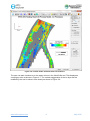
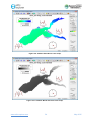
Output from the ice sub model can be displayed in a number of ways in EE. A 2D plan view
of the ice thickness or temperature may be viewed by selecting ViewPlan and then Viewing
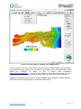
Options | Heat: Bed/Ice. Figure 2-6 shows an example of frazil ice formation in a river in
Alberta, Canada. Note that initially ice forms on the river banks where depths are shallower
and flow is lower.
www.efdc-explorer.com
8
May 2015
Figure 2-6 Ice Sub model: ViewPlan frazil ice thickness.
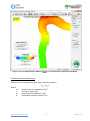
The user can also visualize ice on the water column in the ViewProfile tool. This displays as
a solid grey color as shown in Figure 2-7. The vertical exaggeration of the ice layer can be
modified by the user to show it more clearly as shown in Figure 2-8.
www.efdc-explorer.com
9
May 2015
Figure 2-7 Ice Sub model: ViewProfile ice cover and WC temperature.
Figure 2-8 Ice Sub model: ViewProfile Options.
www.efdc-explorer.com
10
May 2015
Ice may also be viewed in 3D with the View3D tool as shown in Figure 2-9.
Figure 2-9 Ice Sub model: View3D ice cover and water surface elevation.
www.efdc-explorer.com
11
May 2015
3 Evaporation and Forced Evaporation Tool
The Forced Evaporation (FE) Analysis capability has been developed to quantify increased
evaporation induced by increased water temperatures due to releases from thermoelectric
power plants. These power plants withdraw cooling waters, which once run through the plant
and are returned/discharged to rivers or lakes at a higher temperature than the ambient
water temperature. This higher temperature water causes additional evaporation (forced
evaporation) from the river or lake. This additional evaporation is counted as water
consumption by regulators as it is no longer available to downstream users.
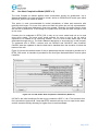
Evaporation is dependent on wind speed, atmospheric humidity, and water temperature.
There are a number of methods to compute FE using different wind functions as listed in
Table 3-1. The wind functions are computed using data contained in the ASER file
(ASER.INP) in EFDC.
Table 3-1 List of Evaporation Calculation Methods
IEVAP
0
1
2
3
4
5
6
7
8
9
10
11
Evaporation Approach
General Usage
Do Not Include Evaporation
Use Evaporation from ASER
Measured or Externally Estimated
EFDC Original
Ward, 1980
Harbeck, 1964
Brady etal, 1969
Anderson, 1954
Webster-Sherman, 1995
Fulford-Sturm, 1984
Gulliver-Stefan, 1986
Edinger etal, 1974
Ryan-Harleman 1974
Cooling Lake
Cooling Lake
Cooling Pond
Large Lake
Lakes
Rivers
Streams
Lakes/Rivers
Lakes/Rivers
Using these various evaporation methods, the model is first run with the power plant, and
then run again without the power plant. EE then subtracts the output from two models and
displays the difference which is the consumption of water from the power plant. The user
may select “with power plant” option to calculate evaporation in the Temperature tab in the
Heat/Temperature frame as shown in Figure 3-1. The evaporation options are only available
if temperature is being simulated and the ASER file is used.
www.efdc-explorer.com
12
May 2015
Figure 3-1 Forced Evaporation: Evaporation Options for Water Balance.
www.efdc-explorer.com
13
May 2015
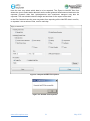
Once the models runs have been completed, the user should go the Model Analysis | Forced
Evaporation tab where the options for model comparison are provided as shown in Figure 32.
Figure 3-2 EE7.3 Evaporation Options GUI
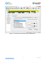
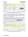
To display the general instructions on how to conduct a forced evaporation (FE) analysis
using EE, click on the blue text box shown in Figure 3-2. EE will display the instructions
shown in Figure 3-3.
www.efdc-explorer.com
14
May 2015
Figure 3-3 FE Analysis Setup Instructions.
As outlined Figure 3-3, the user should then load the With Plant model as the primary (1)
model. Next load model (2) using the Load Without Plant Model button shown in Figure 3-2.
This will display the form shown in Figure 3-4. After selecting Enable Model Comparisons,
two models will have been loaded that can be used for the FE calculations and reporting by
EE.
Figure 3-4 EE7.3 Evaporation Options GUI.
www.efdc-explorer.com
15
May 2015
The Model Labelling frame in Figure 3-2 tells the user the type of FE option that has been
selected. In Figure 3-2, “RH with Plant” refers to model run that used Ryan-Harleman
approach. Time series plots may be automatically generated for either evaporation (no plant)
and forced evaporation (with plant) using the buttons in the respective frames. A plot of
forced evaporation (mm/day) and cumulative volume of forced evaporation is shown in
Figure 3-5.
The user can also produce summaries of evaporation and forced evaporation using the
Tabular Summary button as shown in Figure 3-2.
Figure 3-5 Time series plots of FE using Anderson evaporation approach for B Steam Plant.
Another way to display the impact of FE between the two models is in ViewPlan. Here the
user should select the Volumes | Evaporation viewing option. Selecting Alt M will toggle on
the Model Comparison tool which allows the user to visualize evaporation/rainfall as “With
Plant” minus “Without Plant” models as shown in Figure 3-6.
www.efdc-explorer.com
16
May 2015
Figure 3-6 Forced Evaporation: Model Comparison using Anderson approach for B Model
Plant.
Forced Evaporation Methodology
Heat flux due to evaporation is given by the following equation:
HE = ρLE E
Where:
HE
ρ
LE
E
Heat flux due to evaporation, W/m2
Density of water, kg/m3
Latent heat of evaporation, kJ/kg
Evaporation rate per unit area, m/s
www.efdc-explorer.com
17
May 2015
HE is computed by the following:
HE = f(W)(ew − ea )
Where
F(W)
ew
ea
Wind function in Watts/m2/millibars
Saturation vapor pressure at the water surface, millibars
Vapor pressure of the air at the current temperature and relative humidity,
millibars
The saturated water vapor partial pressures (e) in millibars are computed as:
e = 10
0.7859+0.03477 T
1.0+0.00412 T
Where
T
Temperature, °C
The atmospheric vapor pressure is computed from the dry bulb temperature to get the
saturated vapor pressure. The actual/atmospheric vapor pressure is computed by:
ea = RH es
The wind function is defined by the following equation, with the coefficients varying
depending on the site conditions. EE provides a series of predefined coefficients from
various studies. The user can also provide their own coefficients, if needed.
f(W) = A + B ∗ W2 + C ∗ W22
Where:
F(W) Wind function in Watts/m2/millibars
W2
Wind speed in m/s at 2 meters above the water, m/s
A,B,C Empirical coefficients based on site conditions
Once temperature is activated and the Surface Heat Exchange Sub-Model option is selected
the user can select which evaporation approach is desired. Even if evaporative losses are
not a major concern, the evaporative mass fluxes should normally be activated for most
models.
Heat flux due to evaporation is always included for the Full Heat and the Equilibrium
Temperature (W2) options.
EFDC_DSI/EFDC_Explorer Forced Evaporation (FE) toolset results have been compared to
the Electric Power Research Institute’s (EPRI) FE estimates. EPRI’s once through cooling
FE analysis for river discharges is based on a USGS report on water consumption by
thermoelectric power plants (USGS, 2013; EPRI, 2013).
www.efdc-explorer.com
18
May 2015
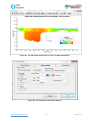
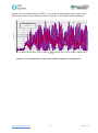
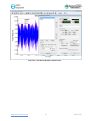
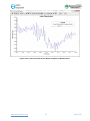
Another new and related feature in EE7.3, is the user can now generate time series of the
differences in water column results as shown in Figure 3-7. DT means “delta temperature”.
Forced Evaporation, Barry Model 2011 - With Plant
3.25
3.00
Legend
2.75
i=47,j=6, Depth Avg DT by EE
DT from Series
2.50
2.25
Temperature (°C)
2.00
1.75
1.50
1.25
1.00
0.75
0.50
0.25
0.00
-0.25
115
125
135
145
155
165
175
185
195
205
215
225
235
Time (days)
Figure 3-7 Forced Evaporation: Time series of model comparison for temperature.
www.efdc-explorer.com
19
May 2015
4 NetCDF Output
EE7.3 now allows the user to export output in NetCDF format. NetCDF (Network Common
Data Form) is a community standard for sharing scientific data. Developed by Unidata, it is
a set of software libraries and machine-independent data formats that support the creation,
access, and sharing of array-oriented scientific data.
EE uses the CF (Climate and Forecast) conventions which Unidata describes as “designed
to promote the processing and sharing of files created with the NetCDF API. The CF
conventions are increasingly gaining acceptance and have been adopted by a number of
projects and groups as a primary standard. The conventions define metadata that provide a
definitive description of what the data in each variable represents, and the spatial and
temporal properties of the data. This enables users of data from different sources to decide
which quantities are comparable, and facilitates building applications with powerful
extraction, regridding, and display capabilities.” http://www.unidata.ucar.edu/software/netcdf/
Figure 4-1 shows the dropdown menu for exporting data from ViewPlan. When the user
selects the Export NetCDF option then form shown in Figure 4-2 is displayed.
Figure 4-1 ViewPlan: Export NetCDF Option.
www.efdc-explorer.com
20
May 2015
Here the user may select which data is to be exported. The Export to NetCDF files form
allows the user to select static data such as the model grid and initial bottom elevations to be
exported. Dynamic data from hydrodynamics and constituent transport may also be
exported. The user should select the begin and end time for the export of the data.
In the File Creation frame the user may select from exporting all the NetCDF data in one file,
or separate it into a series of files, one for each day.
Figure 4-2 Export NetCDF Files Options.
Figure 4-3 NetCDF Files Exported
www.efdc-explorer.com
21
May 2015
4.1
Displaying NetCDF data in ArcGIS
Many tools are available for displaying NetCDF output, these include VisIt
(https://wci.llnl.gov/simulation/computer-codes/visit) , ncWMS etc. This guide will outline
some of the approaches available using ESRI’s ArcGIS. The ability to time-enable spatial
data is available in ArcGIS10.0 and this version is referred to below. The ArcGIS
Multidimensional Tools have three tools that can display NetCDF data:
1. Make NetCDF Raster Layer
2. Make NetCDF Feature Layer
3. Make NetCDF Table View
The menu to access these tools is shown in Figure 4-5.
Figure 4-4 Error! Reference source not found.Multidimensional
ools.
Because NetCDF file can contain many types of data, these tools provide significant
flexibility. The user can choose the best way to represent NetCDF data, as a raster, as a
feature or as a table. For example, it is recommended to view spatial temperature or
precipitation as a raster surface, and use a feature layer to represent point pattern analysis.
The table view may be used when data is not associated with spatial coordinates, such as
fluctuation of water level at a particular gauge.
4.1.1. Visualizing NetCDF data
When NetCDF data is extracted from a curvilinear grid such as those in EFDC models the
tool “Make NetCDF Raster Layer” does not produce a correct grid as raster data must be
spaced in the x and y directions. Instead, it is advised to use the tool “Make NetCDF Feature
Layer” then interpolate with the points feature to a raster using “Spatial Analysis Tool” in
ArcMap.
The following steps will demonstrate how to add a NetCDF file, process it using “Make
NetCDF Feature Layer” tool in ArcMap and then use several tools to create raster datasets.
www.efdc-explorer.com
22
May 2015
It will outline how to create an ArcMap model using the “ModelBuilder” tool to generate raster
datasets at different time steps. The raster datasets can then be animated using “Time
Slider”” tool.
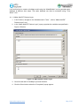
4.1.1.1 Make NetCDF Feature Layer
1. In ArcToolbox, navigate to the “Multidimension Tools” , click to “Make NetCDF
Feature Layer” tool.
2. In the “Make NetCDF Feature Layer” popup, populate the variables as specified in
Figure 4-5 below.
Figure 4-5 Make NetCDF Feature Layer.
3. Click OK and wait for ArcMap to process the data.
4. Click the Close button when the “Completed” popup appear
www.efdc-explorer.com
23
May 2015
4.1.1.2 Create a New Model Using ModelBuilder
A basic knowledge of ArcGIS ModelBuilder is required to fulfill the following steps.
1. In ArcCatalog click New > Toolbox
2. Right click at the new toolbox just created and select New > Model
3. Right click at the new model and select Properties. Type in the name, label and
description for the new model.
4. Right click on Model then select Edit: a white frame will appear in which to set out the
model.
5. In the “Table of Contents”, drag and drop the Feature just created from the NetCDF
file to our Model
6. Go to Search and find the following tools:

Select “By Dimension” (in Multidimension Tool)

“IDW” (in Spatial Analysis Tool)

“Extract by Mask” (Spatial Analysis Tool)
Drag and drop all these tools to the model.
7. Connect the above three tools so they follow the workflow annotation in the Figure 46.
8. Make variables for each tool
9. Specify the necessary model parameters
10. Rename parameters if needed
www.efdc-explorer.com
24
May 2015
Figure 4-6 Work flow of the model.
www.efdc-explorer.com
25
May 2015
Figure 4-7 Finished Model interface.
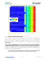
4.1.1.3 Animate the Outputs
If the “Dimension Value” is selected to be different each time, this model will generate a
different raster dataset referred to the select time value. For this particular example, we are
creating 24 raster datasets and viewing this series of rasters according to a timeline to
produce the visual effect of 24 hours variation of salinity in the study area.
Steps:
1. Create a new mosaic dataset and add in the rasters just created
2. Open the attribute table of the mosaic dataset footprint.
3. Add a new ‘date’ type field.
4. Populate the field with the time values. Date time format in ArcGIS is recommended
to be: MM/DD/YYYY HH:MM:SS
www.efdc-explorer.com
26
May 2015
5. Enable time on the mosaic dataset by right-clicking on the mosaic dataset >
Properties > Time tab and check the option: Enable time on this layer
6.
Adjust the time step interval in the Time Tab, we can let ArcMap calculate an interval
by clicking the button “Calculate”
7. Click OK to quit “Layer Properties”
8. Open “Time Slider” window from the “Toolbar”
9. Click the “Play” button or use the time slider to view each raster in the mosaic dataset
as shown in Figure 4-8.
Figure 4-8 Generated raster datasets in ArcMap.
www.efdc-explorer.com
27
May 2015
5 Waves Functionality Updates
5.1
Waves Tab
Bed shear stress associated with waves is an important parameter that contributes to
sediment resuspension and transport process in coastal shallow areas and along shorelines.
EFDC_Explorer has two options for incorporating waves in the flow model. These are
internal wave model and external wave model as shown in Figure 5-1.
The internal wave model internally computes the wind-induced waves using wind data
provided in the WSER.INP file. In contrast, the external wave model requires the output
results from SWAN, Ref/Rif, STWAVE and other wave models. EE will then generate the
WAVE.INP and WAVETIME.INP files from output results to couple with EFDC model.
For all wave models, the user has the option of simulating radiation shear stress with the
Include Radiation Stress check box as shown in Figure 5-1.. Checking or unchecking this
option will change the wave parameters required in the right hand frame.
Figure 5-1 Waves Tab: Internal/External Linkage to SWAN Wave Model
5.1.1. Wave Models in EFDC
The wave model within EFDC uses a naming convention as follows:

No Wave Effects (ISWAVE=0)

External Linkage–Boundary Layer Only (ISWAVE=1, requires WAVEBL.INP and
WV00N.INP, n=1, 2, 3… for version EE7.0, and uses a new format of WAVE.INP for
EE7.1 and later. Refer to the EE7.2 guide for this format).

External Linkage–Boundary Layer and Currents (ISWAVE=2, requires the new
format of WAVE.INP, the same input file as for ISWAVE=1)
www.efdc-explorer.com
28
May 2015

Internally Generate Windwaves – Boundary Layer Only (ISWAVE=3) (EFDC_DSI
only)

Internally Generate Windwaves – Boundary Layer and Currents (ISWAVE=4)
(EFDC_DSI only)
5.1.2. Internal Wave Model Option
In general the influence of wind on the flow velocity field is important while studying
hydrodynamics and sediment transport in lakes, estuarine and coastal areas. Wind effects
not only induce the flow current, but also generate surface waves with a wave height up to
several meters. To calculate the total bed shear stress in such areas, the model must take
the wave factor into account. The wave parameters such as wave height, wave direction and
wave period are calculated by the SMB (Sverdrup, Munk and Bretschneider, see Zhen-Gang
Ji, 2008) model. The wave direction is the same as the wind direction. This means that the
effects of refraction, diffraction and reflection are not taken into account in this internal wave
model.
The internal wave model option doesn’t require imported external wave to simulate wind
generated wave effects on bed shear stress and wave induced currents (Dang Huu Chung
and P.M.Craig, 2009). The fetch for each cell by wind sector may be viewed in ViewPlan
(see Section Error! Reference source not found., ViewPlan Main Viewing Options).
The Wave Parameter & Options form allows the user to specify Ks, the Nikuradse sand
roughness value as shown in Figure 5-1. This can be estimated as Ks = 2.5 x d50. The
Nikuradse roughness is not the same as the hydrodynamic roughness (i.e. bottom
roughness, Z0) used by EFDC to solve the hydrodynamic equations. The Nikuradse
roughness is a grain roughness and represents more of a local scale phenomenon.
For the cases of ISWAVE=3 and ISWAVE=4, available only in EFDC_DSI, the wind time
series provided in the WSER.INP file is used to compute the instantaneous values of wave
parameters with fetch calculated for each cell in sixteen directions. The effect of shoreline
and EFDC internal masks are included in the fetch calculations. The resulting wave
parameters are then used to calculate total bed shear stress, with bed shear stress linked to
the current generated shear stress via the Grant Madsen approach.
From EE5 there has been the ability to internally generate wind-induced wave for bed shears
only (ISWAVE=3). This can also include the radiation stresses for the whole water column
(ISWAVE=4). These options allow the simulation of wave effects and re-suspension of
sediments inside EE.
www.efdc-explorer.com
29
May 2015
5.1.3. External Wave Model Option
This external wave model option allows the user to import wave parameter fields from other
common wave models. The Steady/Unsteady option corresponds to the types of waves
being imported into the EFDC model. The steady wave option means that the waves are not
changing with time so the EE will not read the WAVETIME.INP file. The unsteady wave
option does require the WAVETIME.INP input file. The setting in the frame reflects the way
the user has imported the external waves.
Figure 5-2 Waves Tab: External Linkage to SWAN Wave Model.
There are four different sub-options to take into account while assigning the wave
parameters into EFDC model as following;
a) Use Wave Input File
If the user already has a WAVE.INP file (of format shown in Appendix B 12), then the data is
imported first time by checking the New Dataset checkbox. If a WAVE.INP has already been
imported then the import options described below are greyed out until the New dataset box
is selected.
b) Import Existing Data
EE imports an available WAVE.INP file from another project into the current project. It should
be noted that two projects must have exactly the same grids.
c) Set Spatially Varying Wave Inputs
This is an option for EE7 and earlier and it is not advised be used due to the longer time
required to prepare the input data. For ISWAVE=1 and ISWAVE=2 the external model
results may be imported into EFDC_Explorer which will generate the required wave linkage
file, depending on the ISWAVE option. Figure 5-3 shows the main import/field interpolation
form for the wave parameters for ISWAVE=2. The user must match the input data file (which
should be in XYZ format tab, space or comma delimited) to the parameter specified on drop
down list Wave Field Parameters (options shown in adjacent inset). The user can either
www.efdc-explorer.com
30
May 2015
have wave height (2*wave amplitude) or wave energy. EE will compute the one from the
other. The user has the option of using a polygon to select which EFDC cells will be used for
the assignment. If a Poly file is not selected, then the assignment operation will be for the
entire model domain. EE interpolates and converts the wave model results into the formats
needed for EFDC. The interpolation process has two options, nearest neighbor interpolation
or cell averaging. Cell averaging should be used when the imported data is denser than the
EFDC model grid (this will usually be the case). The nearest neighbor interpolation scheme
should be used if the imported data is sparser than the EFDC model grid.
Wave Properties to be
imported.
Figure 5-3 Wave generated turbulence, import data form.
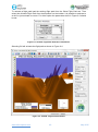
DSI has extensively tested and verified the ISWAVE=2 option for both EE and EFDC using
the RefDif/ShoreCirc modeling of rip tide currents (Svendsen, et. al., 2000). Figure 5-4
shows EFDC_DSI model results for the rip tide test case. The velocity vectors (in white)
have been overlaid on the bathymetry. The velocity pattern and magnitude are similar to
what was computed by Svendsen.
www.efdc-explorer.com
31
May 2015
Figure 5-4 Wave generated rip tide currents overlaid on idealized beach.
d) Import Wave Model Results from SWAN
Currently EE only imports data from the SWAN wave model, however, it is anticipated that
other models will be included at a later date. If the user chooses to import the SWAN output
files through EE then the Import Wave Model (SWAN) button should be selected. This
displays the form shown in Figure 5-5. The default Work Path is the current model directory.
The user should browse to a different directory if they want to avoid saving over an existing
WAVE.INP file.
In the Import from SWAN frame the user should first decide if they are using steady or
unsteady waves with the dropdown box. If steady waves are used then then EE does not
require the WAVETIME.INP file as the waves are at regular time intervals and the option to
load this file is disabled. Alternatively, if unsteady waves are being used then then browse to
the path for the SWAN model outputs and select the the wave time file (WAVETIME.INP).
Next there are two options for SWAN input:
1. Using output for locations option requires the SWAN model to have same grid as
the current EE modeland uses the group file from SWAN, (SWAN_GRP.INP).
www.efdc-explorer.com
32
May 2015
2. Using output for location option uses the data as x, y points. This option should be
chosen when SWAN and EE use two different grids and wave data was exported at
the locations (x, y) from the SWAN model. The latter option requires two input files: a
location file and a table file. These should have been defined and saved out from the
SWAN model.
Once these files have been selected the user should select the Import button. Two files will
be created: WAVE.INP and WAVETIME.INP for the EFDC model run.
Figure 5-5 Waves Tab: SWAN Import function when using same grid as EE.
5.1.4. Creating SWAN Model Output – Running SWAN from EE
A new feature in EE7.3 is the ability to build input files for SWAN and then run SWAN
directly from EE. Note that this is not fully integrated dynamic coupling between SWAN and
the EFDC model at this stage. Instead, EFDC will use the final SWAN output as input for the
external wave model.
The steps to run SWAN from EE are as follows. First it is necessary to create a SWAN input
file. This is done in ViewPlan under the Export Data dropdown button, and selecting Export
SWAN as shown in Figure 5-6. After selecting this option, the Export to SWAN file from is
opened as shown in Figure 5-7
www.efdc-explorer.com
33
May 2015
Figure 5-6 External Waves: ViewPlan Export SWAN Option.
The user should select which input data is required for their SWAN model. The Parameters
button provides further options for the creation of the SWAN inputs. The SWAN user guide
should be consulted for details on how to select these parameters
(http://www.swan.tudelft.nl/). If the user also intends to export the wind series for use in
SWAN, the start and end times should be selected as well as the time step for this data.
Navigate to the folder that you want to create the SWAN input files with the SWAN Working
Path frame before selecting Export to create the SWAN inputs.
www.efdc-explorer.com
34
May 2015
Figure 5-7 External Waves: Export SWAN Input File from EE.
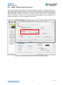
Once the SWAN input files have been created the user should proceed to the Waves tab on
the main EE form. When External Wave Model option has been selected and the Create a
New Data Set is not selected, the Run SWAN option is displayed. As explained earlier, this
provides the option of running SWAN directly from within EE (though not at the same time as
EFDC is running i.e. it is not dynamically linked).
Selecting the SWAN Run button displays the form shown in Figure 5-8. The user should
browse to the work path for the SWAN input files if necessary. The user should then browse
to the SWAN executable file. The SWAN exe is installed as part of the installation package
for EE. SWAN is freeware under the GNU license and the executable and source code may
be downloaded from the University of Technology, Delft http://www.swan.tudelft.nl/
The user should the select the Run SWAN button to run the SWAN model. After the SWAN
model has finished running the user should select the Create a New Data Set checkbox and
use the Import the Wave Model Results feature to import SWAN output in to EE.
Figure 5-8 External Waves: Run SWAN internally from EE.
www.efdc-explorer.com
35
May 2015
5.1.5. Use SWAN Model Output
The user also has the option of importing the SWAN model outputs directly into EFDC
(Figure 5-9). This requires the SWAN user to select either a location file (table) or for a grid
file (group) which can be exported from SWAN. Once again the user should know if they are
importing steady waves or unsteady waves and select the appropriate option from the
dropdown box. The output files names from SWAN should be saved as:
SWAN Location file:
SWAN_LOC.INP & SWAN_GRP.INP or
SWAN Table file:
SWAN_TBL.INP
The radial buttons in form USE SWAN Model Output allow the user to select which type of
input file is being input. The EFDC.INP is then updated to tell EFDC which will then look for
the appropriate files in the root level of the project directory.
Figure 5-9 Waves Tab: Use SWAN Model output.
www.efdc-explorer.com
36
May 2015
6 Flight Path Animation
The flight path animation tool allows the user to define and edit a flat path and then create an
automated animated sequence through the model domain in View3D. To create a flight path
select Show/Hide Flight Path Tools from the dropdown menu as shown in Figure 6-1. Using
the controls now displayed the user may define, save, load and edit a flight path.
Figure 6-1 View3D: Flight Path Animation.
Controls for the flight path are used to draw a spline that can be either a straight line or a
curved line and must contain at least two points. In the main toolbar there are a number of
icons that may be used to define the flight path that are explained in Table 6-1.
www.efdc-explorer.com
37
May 2015
Table 6-1 Flight Path Polyline Tool Buttons.
Open an existing flight path polyline.
Save a flight path polyline. It is necessary to select this icon for the
polyline to be saved.
Define a new flight path. LMC in the workspace creates a point. Moving
the mouse and LMC in another location creates another point with a
line joining the two points. RMC to end drawing the polyline.
Delete previously created line. When this icon is selected, clicking on a
line will delete it.
Insert points on an already created line. Once a point is inserted it can
be moved to reshape the line.
Move points on a polyline.
Delete points on a polyline.
Edit a point. Edit the x, y, z location of a point as well as the roll.
Assign a constant elevation to the flight path. Sets all the vertical
elevations of the flight path at one time as opposed to editing it point by
point.
The process for creating a flight path are as follows:
1. Select the flight path tool drop down Show Flight Path Tool
2. EE will reset to plan view to draw the flight path in the horizontal plan view
3. LMC on the first point of the path and LMC for each subsequent point on the path
4. RMC to end the line
5. Move or delete points as required using the Move and Delete buttons. Note that it is
not possible to pan in this mode except by using the arrow keys
6. Select the Z button to set the vertical position of the flight path
7. Use the Edit Point button to further adjust the vertical position or roll of any point
8. Rotate the model to ensure the flight path is vertically and horizontally correct
9. Save the flight path
www.efdc-explorer.com
38
May 2015
A number of options are available to user to define the flight path. These options are
available from the Animate Flight Path from the dropdown on the toolbar and shown in
Figure 6-2. The user can first decide whether or not to display the flight path polygon using
the Show check box. It is also possible to adjust the animation steps to provide a smoother
visualization. Camera height and angle may also be set. FovY is field-of-view in the y
dimension i.e. vertical angle, which may be set to maximize the image size on the screen.
The user may select various options for the path color when editing the lines as well as
colors displayed when a line is selected or dragged.
The user can select the spline type to be used for the flight path. The default is the Catmull–
Rom spline in which the original set of points make up the control points for the spline curve.
“B spline” may also be selected, in which the curve does not remain on the original control
points. The user may also select the spline checkbox to switch on or off the use of splines.
Figure 6-2 View3D: Flight Path Options
www.efdc-explorer.com
39
May 2015
To animate a flight path load the existing flight path from the Show Flight Path tool. Then
select the Animate Flight Path from the dropdown on the toolbar. It is possible to animate to
an AVI or just animate to screen. For either option the parameters show in Figure 6-3 should
be set.
Figure 6-3 View3D: Flight Path Animation Parameters.
Selecting OK will animate the flight path as shown in Figure 6-4
Figure 6-4 View3D: Flight Path Animation.
www.efdc-explorer.com
40
May 2015
7 Automated Atmospheric and Wind Series Weighting
EE previously had the ability to add multiple wind and atmospheric stations and provide a
user defined weighting to each station. Now it is possible to automatically weight the multiple
series based on their distance from the model domain.
To set the coordinates of the wind series, click the Show Parameters button in the Wind BC
Time Series Editing; or to set coordinate of the atmospheric series, in the Atmospherics BC
Time Series Editing tool as shown in Figure 7-1 and Figure 7-2. EE will use the X, Y
coordinates in the value column. If the user has not entered the X, Y values then EE will
automatically calculation X,Y coordinates based on the lat/long values provided. However, if
both are entered it should be noted that EE will use the X, Y coordinates. The user can also
set the anemometer height of the station.
Figure 7-1 Wind Data Series: Station Coordinate Setting.
www.efdc-explorer.com
41
May 2015
Figure 7-2 Atmospheric Data Series: Station Coordinate Setting.
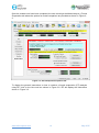
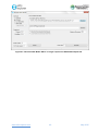
The user should now select the Series weighting button from either Temperature |
Atmospheric Data for atmospherics or from Hydrodynamics | Wind Data for winds. To set the
spatial weighting, select the Generate Using Station Coordinates radial button as shown in
Figure 7-3.. XYZ interpolation options can be set in terms of the number of sectors and
inverse distance power. An example of wind weighted stations displayed in ViewPlan is
shown in Figure 7-4.
www.efdc-explorer.com
42
May 2015
Figure 7-3 Atmospheric Series Weightings: Automatic Option.
www.efdc-explorer.com
43
May 2015
Figure 7-4 ViewPlan: Automatic Wind Series Weightings.
www.efdc-explorer.com
44
May 2015
8 Elimination of Template Files
From the release of EE7.3 the master input files for EFDC will be stored in a non-editable
database. EFDC_Explorer automatically updates the EFDC default initial conditions from an
MS Access file for the following files:
 EFDC.INP
 WQ3DWC.INP
 WQ3DSD.INP
 WQRPEM.INP
The user can then modify the model as necessary using EE. An example showing the the
generation of a new model with the the former method for inputting the template file is shown
in Figure 8-1 and the new method in Figure 8-2.
Figure 8-1 Generate New Model: EE7.2 and earlier prompt for EFDC.INP template file.
www.efdc-explorer.com
45
May 2015
Figure 8-2 Generate New Model: EE7.3 no longer requires the EFDC.INP template file.
www.efdc-explorer.com
46
May 2015
9 Miscellaneous Updates
9.1
Export Toxics in Tecplot Update
EE has been updated to enhance the Tecplot export functions for different parameters.
Previously EE only had an option to export toxics to Tecplot for the sediment bed. EE now
allows users to export the water column parameters in addition to bed directly to Tecplot.
The Tecplot export function in Water By Layer and Water By Depth option has also been
implemented. When exporting the sediment bed toxics EE exports the real values and does
not truncate the output. The dropdown to select this function is shown in
Figure 9-1.
Figure 9-1 ViewPlan: Export toxics in the water column to Tecplot.
www.efdc-explorer.com
47
May 2015
9.2
3D Symbols
EFDC_Explorer7.3 can now display symbols as 3D images. These are selected in the
normal way from Display Options | Annotations | Edit Labels | Edit (Selected Labels) as
shown in Figure 9-2 and Figure 9-3.
Figure 9-2 View3D Display Options: Configuring 3D symbols.
Figure 9-3 View3D Display Options: 3D triangle symbol.
www.efdc-explorer.com
48
May 2015
9.3
Buffer loading for EE drifters
EE7.3 now implements buffers for loading the EE_DRIFTER files. This option significantly
increases the loading speed of model which uses the LPT sub model. The user may now
use very large numbers of drifters without experiencing appreciable slow down when loading
the model. This follows the typical EE linkage file use of binary buffers to load model results.
9.4
Subscript and Superscript in Graph Legends
The Time Series Grapher and EFDC Profile tools have been updated to display user defined
subscripts and superscripts in the legends. This is done using two underscore key strokes
(“__”) and a single caret (“^”) for subscripts and superscripts respectively. An example of
implementing subscripts and superscripts is shown in Figure 9-4. If several characters are
part of a group they should be placed in curly brackets (“{ }”). For example to display: x2 +
log2x + log10x, the user should write x^2 + log__2x + log__{10}x as the label as shown in
Figure 9-4.
Figure 9-4 Time Series Grapher: adding subscripts and superscripts.
www.efdc-explorer.com
49
May 2015
9.5
Delete Lines from Line Options (Time Series Grapher)
EE7.3 now provides the options to delete (rather than just turn off or hide) lines from the
Time Series Grapher tool. This is shown in Figure 9-5 where the user has selected two
lines. Then by selecting the Delete button the lines are removed from the legend, from the
display and the Line Options and Controls menu as shown in Figure 9-6.
Figure 9-5 Time Series Grapher: Deleting lines.
www.efdc-explorer.com
50
May 2015
Figure 9-6 Time Series Grapher: Deleted lines.
www.efdc-explorer.com
51
May 2015
9.6
Display Miles or Feet in Labels
EE7.3 now allows the users to display graph/plot labels in metric or British imperial units
using the CTRL M keystroke to toggle the units. Selecting ALT M will toggle the x axis from
feet to miles. An example of the graph in imperial units is shown in Figure 9-7.
Figure 9-7 Water Surface Profiler: Imperial units display toggle.
www.efdc-explorer.com
52
May 2015
9.7
Specify Color Ramps
EE7.3 provides the user with a number of options for displaying the color ramps in ViewPlan
and View3D. The typical choice is the temperature color ramp which shows blue for low
values and red for high values. Many other color ramps are now available as shown in
Figure 9-8. Examples of the blue green and black and white color ramps are shown in Figure
9-9 and Figure 9-10 respectively.
However, if the user selects Single Color from the dropdown then the color ramp will use a
gradient based on the Single Color option selected beneath the drop down list. If Solid Color
is selected then only that color is used and it is shaded based on lighting effects if selected.
Figure 9-8 View3D: Color ramp options.
www.efdc-explorer.com
53
May 2015
Figure 9-9 ViewPlan: Blue-Green color ramp.
Figure 9-10 ViewPlan: Black and white color ramp.
www.efdc-explorer.com
54
May 2015
9.8
Particles on the boundary disappear in 3D
In the particle tracking submodel of earlier versions of EE, particles that reach the model
boundary stick to the edge of the boundary as shown in Figure 9-11. This is to show that the
particles have left the model domain and are no longer being calculated. In EE7.3 a new
method has been added which provides the user an option to allow the particles to
disappear if the the Hide After Exit check box is selected as shown in Figure 9-12.
Figure 9-11 View3D: Oil spill still displayed after exiting model domain.
www.efdc-explorer.com
55
May 2015
Figure 9-12 View3D: Oil spill hidden after exiting model domain.
www.efdc-explorer.com
56
May 2015
9.9
Change Legend Font Sizes
EE7.3 now provides the user with the option of adjusting the font, color and size of the text
label in the legend in ViewPlan. This can be achieved by using ALT- F and selecting options
as shown in Figure 9-13
Figure 9-13 ViewPlan: Adjustable legend front sizes.
www.efdc-explorer.com
57
May 2015
9.10
Display Wind and Atmospheric Stations in ViewPlan
EE now has the capability to display the atmospheric, wind and ice stations in ViewPlan. If
the ASER, WSER or ISER co-ordinates are not populated then EE will automatically use the
centroid of the model domain as shown in Figure 9-14. The coordinates of these are now
stored in the .EE file. The ASER location is used by EFDC to calculate solar radiation. Figure
9-15, Figure 9-16 display the wind series plot (View Wind) and wind series data (Edit Wind)
that are generated from the first two display options in Figure 9-14.
Figure 9-14 Wind Data Series: Station Coordinates in ViewPlan.
www.efdc-explorer.com
58
May 2015
Figure 9-15 Wind Data Series: Time Series of wind magnitude and direction.
Figure 9-16 Wind Data Series: Station Coordinate Setting.
www.efdc-explorer.com
59
May 2015
9.11
WSER, TSER and ISER Timeblocks
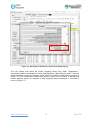
Time blocks for time series has now been implemented in EFDC. This allows the user to
adjust the weighting for each series over time to better represent that relative accuracy of
each station. For example, in Figure 9-17, time block 1 is set from 5113 to 5130. The wind
weight distribution obtained by using the feature Generate Using Station Coordinates is
shown in ViewPlan in Figure 9-18. This figure also demonstrates how the locations of the
wind series stations can now be displayed in ViewPlan.
Figure 9-17 Atmospheric Data Series: Station Coordinate Setting.
www.efdc-explorer.com
60
May 2015
Figure 9-18 Atmospheric Data Series: Station Coordinate Setting for Time Block 1.
A second time block, from 5130 to 5478 has also been set with the Use Constant option and
the following proportions: Concord=0.2; Sacramento=0.3 and Stockton=0.5 as shown in
Figure 9-19 and Figure 9-20.
www.efdc-explorer.com
61
May 2015
Figure 9-19 Atmospheric Data Series: Station Coordinate Setting.
www.efdc-explorer.com
62
May 2015
Figure 9-20 Atmospheric Data Series: Station Coordinate Setting for Time Block 2.
9.12
Automatic Seat Deactivation
EE will now automatically prompt the user to deactivate EE if they attempt to uninstall EE
while there is still an active seat.
www.efdc-explorer.com
63
May 2015
9.13
Date and Coordinate Conversion Tool
A new feature has been added to EE7.3 in ViewPlan for the purpose of converting dates and
coordinates. This tool is accessible from the same location the tool for converting between
Julian and Calendar dates was previously available, however the button has been updated
as shown in Figure 9-21. The Date Conversion tab is the same as for EE7.2. Two new tabs
have been added: IJ / XY Conversion and UTM Conversion. The former of these is shown in
Figure 9-21. An L index or IJ pair can be entered into the text box and EE will automatically
display the corresponding L, IJ or model grid coordinates.
Figure 9-21 Date and Coordinate Conversions.
The user may also select the UTM Conversion tab to convert from longitude and latitude
coordinates to UTM or vice versa. The user should enter the coordinates in the text box and
ENTER keystroke for this conversion to take place as shown in Figure 9-22. The user may
also copy this information to the clipboard with the Copy to Clipboard button. A file
containing coordinates may also be converted using the Convert File button and browsing to
the file to be converted.
www.efdc-explorer.com
64
May 2015
Figure 9-22 Date and Coordinate Conversions.
9.14
Display Model Comparisons in Time Series
When a user has a comparison model loaded (see User Manual for EE7.2 for details) in
EE7.3 it is now possible to select Alt-M in ViewPlan to compare the model results as shown
in Figure 9-23. In versions prior to EE7.2 the time series extraction would only be for the
base model. However, in EE7.3 the time series extraction is the Base – Compare models as
shown in Figure 9-24.
www.efdc-explorer.com
65
May 2015
Figure 9-23 ViewPlan: Model Compare for WS Elevation.
www.efdc-explorer.com
66
May 2015
Figure 9-24 Time Series Extraction: Model Compare for WS Elevation.
www.efdc-explorer.com
67
May 2015
10 Appendix Data Formats
www.efdc-explorer.com
68
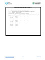
May 2015
Data Format B-16 ISER.INP for ISICE = 1
C ** PROJECT NAME, ISER.INP TIME SERIES FILE
C **
FILE ISER.INP - EXTERNALLY SPECIFIED ICE COVER
C **
CONTROL AND TIME SERIES DATA REPEATING NISER TIMES.
C **
HEADER: MISER(NISER),
TCISER(NISER),TAISER(NISER),RMULADJC,RMULADJT
C **
MISER
= NUMBER OF DATA, TCISER=TIME CONVERSION TO SEC,
TAISER=ADDITIVE TIME ADJ
C **
4
86400
0
1
0
240.001
0.3500
240.010
0.5500
240.020
0.7500
240.030
0.6000
6
86400
0
1
0
20.000
0.0000
238.000
0.4000
252.000
0.5700
283.000
0.7200
290.000
0.5500
320.000
0.3400
www.efdc-explorer.com
69
May 2015
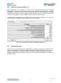
Data Format B-17 ICEMAP.INP for ISICE = 1
C ** , icemap.inp , Ice time series weightings for each cell and NISER
Series
C **
C **
C
I
J
Weighting Fraction by Series
1
5113.000 5478.000
2 107
3 0.000159 0.999672 0.000170
3 108
3 0.000159 0.999671 0.000170
4 109
3 0.000159 0.999671 0.000170
5 110
3 0.000160 0.999670 0.000170
6 107
4 0.000231 0.999520 0.000249
7 108
4 0.000232 0.999519 0.000249
8 109
4 0.000232 0.999518 0.000250
9 110
4 0.000233 0.999517 0.000250
10 107
5 0.000313 0.999346 0.000341
11 108
5 0.000315 0.999344 0.000341
12 109
5 0.000316 0.999342 0.000342
13 110
5 0.000317 0.999340 0.000343
14 107
6 0.000413 0.999135 0.000453
www.efdc-explorer.com
70
May 2015
Data Format B-18 ISTAT.INP for ISICE = 2
C
C
C
C
C
**
**
**
**
**
ISTAT FILE
TIME SERIES ON THE STATUS OF ICE ON/OFF VIA ICECOVER
FIRST DATA LINE: MISER(N),TCISER(N),TAISER(N),N=1(only one)
NEXT DATA LINES: TISER(M,N),RICECOVS(M,N), M=1:MISER
TISER: TIME, RICECOVS = 1: ON/0:OFF
5
86400
0
0.000
0.0000
240.000
1.0000
242.000
0.0000
243.000
1.0000
300.000
0.0000
www.efdc-explorer.com
71
May 2015
Data Format B-19 ICE.INP for ISICE = 3 & 4
* ICE THICKNESS INITIAL CONDITIONS
*
*
I
J
THICKNESS[M]
3 207
0.300
3 208
0.300
3 209
0.300
3 210
0.300
3 211
0.300
3 212
0.300
4 207
0.300
4 208
0.300
4 209
0.300
4 210
0.300
4 211
0.300
4 212
0.300
5 207
0.300
5 208
0.300
www.efdc-explorer.com
72
May 2015
11 References
Evaluating Thermoelectric, Agricultural, and Municipal Water Consumption in a National
Water Resources Framework, EPRI, 2013
Methods for Estimating Water Consumption for Thermoelectric Power Plants in the United
States, USGS, 2013
www.efdc-explorer.com
73
May 2015