Download Demonstration Manual Version 8.7

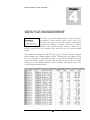
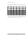
Demonstration Manual Version 8.7
User manual designed by:
 Sanitas Technologies
22052 W. 66th Street, Ste. 133 ● Shawnee, KS 66226
Phone 913.829.1470; Fax: 831.854.1470
www.sanitastech.com
Email: [email protected]
i
SANITAS™ FOR GROUND WATER
DEMONSTRATION MANUAL
Information in this document is subject to change without notice and does not represent a
commitment on the part of Sanitas Technologies (formerly known as Intelligent Decision Technologies,
Ltd. and NIC). The software described in this document is furnished under a license agreement and may
be used only in accordance with the terms of the agreement. No part of this manual may be reproduced
or transmitted in any form or by any means, electronic or mechanical, including photocopying, recording,
or information storage or retrieval systems, for any purpose other than the purchaser’s personal use
without the permission of Sanitas Technologies.
© 1992-2007 Sanitas Technologies. All rights reserved.
Windows and Windows® 95, 98, 2000, NT, ME, XP, and Vista are registered trademarks of
Microsoft Corporation.
No investigation has been made of common-law trademark rights in any word.
Sanitas Technologies makes no warranties, either express or implied, regarding the enclosed
computer software package or its fitness for any particular purpose.
™
Table of Contents
INTRODUCTION..................................... 1
SYSTEM REQUIREMENTS .................. 3
INSTALLING SANITAS ......................... 3
BASIC CONCEPTS.................................. 5
DATA FILE MANAGEMENT................ 6
SANITAS™ FUNCTIONALITY ............ 8
ANALYSIS DIRECTORY ..................... 13
ONLINE HELP....................................... 16
SANITAS™ LICENSE PRICES ........... 17
D E M O N S T R A T I O N
M A N U A L
Chapter
1
INTRODUCTION
Demonstration Version
W
elcome to the Demonstration Version of Sanitas™ for Ground Water. We
hope this demonstration manual and Sanitas online help will aid you in
rapidly installing Sanitas and exploring its features. Online help can be
accessed through the Windows Start Menu, or through the Sanitas Main
Menu (Help/Sanitas Manual). If you have any questions or comments, please contact
Sanitas Technologies at 913.829.1470 or [email protected].
The purpose of this demonstration manual is to get you up and running rapidly so you
can explore the features that Sanitas has to offer. We have included a section that will
walk you through several exercises (page 8) to get you started. This demonstration
manual is not the standard Sanitas User Manual. If you have questions that cannot be
answered by this manual or Sanitas online help, please feel free to contact us.
Sanitas for Ground Water, the In-House Compliance Expert system, automates the
statistical analysis of RCRA hazardous waste (Subtitle C) and municipal (Subtitle D)
landfill ground water quality data. Sanitas was designed to significantly reduce analysis
costs and minimize errors that can lead to increased monitoring costs.
Sanitas helps ensure that a facility’s ground water quality statistical analysis procedures
meet EPA and state regulations. The program's decision logic identifies the
appropriate analysis procedure options that are available under the applicable
regulations, then guides the user through the running of those analyses. Its data format
and built-in data translator simplify data entry and management requirements, and it
provides screen and hard copy plots as well as reports that can be submitted to clients
and/or regulators.
1
D E M O N S T R A T I O N
M A N U A L
SANITAS
VERSION
8.7
Upon purchase of Sanitas Version 8.7,
you will be provided with a link to download the software
which includes a complete user manual that provides detailed
descriptions
and examples of the statistical methodologies
General information
offered in Sanitas. Alternatively, a customized installation
CD and hard copy manual may be requested for an additional cost.
A number of other topics are covered in the manual, including:
•
•
•
•
•
the installation of Sanitas;
the data file structure requirements;
the data file translator;
troubleshooting solutions;
a description of RCRA statistical procedures incorporated into
Sanitas; and,
• examples of various statistical procedures.
The facility specific license also includes one year of unlimited telephone/email
software support and free upgrades, and 90 minutes of telephone/email statistical
support by Sanitas Technologies’ staff of statistical experts. You will recieve periodic
Sanitas newsletters that highlight user tips and statistical suggestions. This newsletter
gives you the opportunity to stay current with changes in Sanitas and a chance to ask
any statistical questions that you might have.
2
D E M O N S T R A T I O N
M A N U A L
Chapter
2
SYSTEM REQUIREMENTS
•
Pentium® 166 processor minimum (Pentium® II 233 or higher
recommended).
•
Microsoft® Windows® 95 Service Release 2. Windows 98,
Windows NT® 4.0, Windows 2000, Windows Millennium Edition,
Windows XP, or Windows Vista.
•
32 megabytes (MB) of random access memory (RAM) (64 MB or
more recommended).
•
70 MB or more free hard disk space.
•
Video graphics adapter (VGA) able to display at least 256 colors at
800 x 600 pixel resolution recommended.
INSTALLING SANITAS
This section describes how to install the software included in the Sanitas
demonstration download. Please read the following instructions before beginning
installation.
1. In WindowsTM, close all applications.
2. Click on Downloads, Sanitas Demo, and click “Open” to begin the installation
process.
3
D E M O N S T R A T I O N
M A N U A L
3. The Setup Wizard will appear. The default path chosen for installation is
C:\Program Files\Sanitas for Groundwater. Either click Next to accept the
default or type the new path and then continue.
4. You will be prompted through a series of screens, in which the default is
generally satisfactory.
5. When the Setup Wizard is complete, you will be prompted to launch the
Sanitas program.
6. Alternatively, to start the Sanitas program through Windows Explorer, go to
Start, Programs, Sanitas for Groundwater and click Sanitas™ for
Groundwater v.8.7.
4
D E M O N S T R A T I O N
M A N U A L
Chapter
3
BASIC CONCEPTS
Only a few basic concepts need to be understood in order to
begin operating Sanitas. The general sequence of operations is:
Select or Add a datafile.
The demo version is unrestricted in terms of the data that may be
analyzed. Please see the online help for data file requirements, if you will
be analyzing your own data.
Select or Create a View.
The Sanitas View window allows you to select a constituent for analysis,
and to choose wells, dates etc. Once such selections have been made, the
matching data is "read into" the View, and the data can be examined
and/or edited. The selected View contains the data that will be analyzed.
Run Reports.
An analysis directory is included in this manual. There is also a batch
feature that allows automation of multiple-report jobs.
Review Results.
In addition to hardcopy reports, summary tables are optionally created
during analysis. A variety of formatting options are available for both the
reports and summary tables.
Helpful Tips:
• Highlighted decision points (nodes) in the decision flow charts are
clickable to access relevant details and/or operations.
•To select or deselect wells, constituents, and/or dates, click on that line of
the scrolling list. The letter to the left of the item indicates whether it is
selected (Y) or deselected (N).
•Global selection/deselection of items is available, with a right click providing
a pop-up menu.
5
D E M O N S T R A T I O N
M A N U A L
Chapter
4
DATA FILE MANAGEMENT
Data files are prepared independently of Sanitas, through a
spreadsheet or other program such as Excel, Access, etc.
Files are prepared in a
All Sanitas data files are text files, typically tab-delimited,
spreadsheet and translated
though
some flexibility is available. Data may be entered
into Sanitas-readable format.
directly in the “Sanitas-readable” format, or Sanitas has a
built-in translator that can translate many data files into the Sanitas-readable
format.
Data File
Translation
The translator can translate an ASCII flat file (a type of data file typically exported
from a database) into a Sanitas-readable text file. The following is an example of a flat
file. It is important to understand that there is a great deal of flexibility in this file
format (for instance, columns and their order, the presence and specifics of column
headers, etc.). For detailed information about particular fields, please refer to the
Online Help in the Sanitas Demo.
Example of Flat File Translatable Format
6
D E M O N S T R A T I O N
M A N U A L
If you wish to prepare a data file in Sanitas-readable format that may be directly added
to the program rather than translating a flat file, the following is an example of that
format:
[XYZ
Landfill]
[3-21a]
[Detection]
[22-oG9]
Dissolved Iron (mg/I) Benzene (ug/I)
n/a
Well#1
Well#2
71-43-2
u
1/1/1991
n/a
n/a
3.4
12.5
4/1/1991
n/a
n/a
<2
<5
7/1/1991
n/a
n/a
n/a
16
n/a
n/a
15
21
n/a
n/a
5.2
20
d
1/1/1991
7/1/1991
Example of Sanitas-Readable Format
The easiest way to enter data in this format is to open and modify an existing Sanitas
data file, such as the data files included with the demo. For detailed information about
particular fields, please refer to the Online Help in the Sanitas Demo.
7
D E M O N S T R A T I O N
M A N U A L
Chapter
5
Sanitas™ Functionality
The purpose of this section is to guide you through the first exploration of Sanitas™.
Understanding data file selection and how to analyze the data
Understanding
are keys to a successful first statistical evaluation.
the Mechanics
Select ing a data file, and
analyzing the data..
In Sanitas, you have the option of analyzing your data using
one of two methods. The Batch method offers you the
opportunity to select multiple wells and constituents for multiple-report runs. The
View method provides an interactive approach for you to analyze individual
constituents and “View” your results, allowing you to create on-screen graphs for
inspection prior to printing. In this exercise, we will explore the View method. Please
ensure that the Summary Tables feature has been turned on, as it is by default, in the
“Configure Sanitas” options, Analysis tab. Summary Tables will be created throughout
this exercise for each of the statistical tests you select. If you are notified that a
Summary Table exists for a particular test, you may “append” each new test so that a
continuous summary of the results may be recorded and reviewed at the end of this
exercise.
•
•
Launch Sanitas and click on the “Start” button
Select a Data File
-Highlight “Demo Inorganic”
-If you would like to analyze your own data, you may do so by clicking the
hyperlink to Add your data file. We encourage you to first step through
this sequence to familiarize yourself with the program.
•
Select an Existing View (“Example View”)
-Highlight “Example View” and then “Open View”
(This View was created for demonstration, and contains data which are
ready for analysis. Please refer to Page 9 to “Create A New View”.)
•
Create a Box and Whiskers Plot
-Choose “Graph” from the Menu bar and select “Box Plot” (A Summary
Table will be created.)
-Click “OK” (If you are notified that outliers may exist in the data set, click
continue so that you may view the Box Plots.)
8
-Return to View by clicking on “Exit”.
•
Alter the View & Examine Individual Observations
- Click on “Examine Observations”.
- Sort the data by clicking “Data” from the Menu bar.
- Choose to “Sort by Well” and examine the changes.
- Click on a line to deselect the observation.
•
Deselect a Well’s Observations
- Click on “Selection Palette” (a sub-window
will appear in the lower right corner).
- The options on the Selection Palette can be changed
by toggling any of the three buttons (1st button:
Select/Deselect; 2nd button: Date/Well ID/
Value/Alt. Value/Flags/All; 3rd button: =/</> or
= ).
- Change the buttons to “Deselect”, “Well-ID”, and
“=”.
- Type “HL-6” in the blank below the buttons.
- Click on “Execute”; All of the data for well HL-6 should now be
deselected; note that the “Y”s on the far left of each line have changed
to “N”s.
•
Plot a Times Series
-Choose “Graph” from the Menu bar and select “Time Series”.
-Click “Continue” when notified that you have more than 5 wells selected.
-Examine the Time Series plot and click “Exit” to return to the View.
•
Reselect all of the wells using the Selection Palette
- Change
the Selection Palette so the top button is on “Select” and the
middle left button is on “All”.
- Press Enter or click on “Execute”.
•
Plot a Seasonality Graph (MW-1)
- Select “Graph” from the Menu bar and select
“Seasonality”, then “OK”.
-Choose well “HL-6” and click on “OK”.
-When Seasonality is determined to be present in a data set, data should be
deasonalized prior to running statistical analyses.
- Exit.
- Select “Yes” or “No” to analyze other wells for Seasonality.
- Click Exit when finished and click on the “Hide” button next to “Examine
Observations” to hide the Observations sub-window.
░When
Seasonality is
present,
Data should typically be
deasonalized prior to
running a statistical
analysis. This may be
accomplished in the
“View” under the
“Data” pull-down
menu.
•
Create a New View
- Exit the current view by clicking “Done”.
- Click “Start” and highlight the “Demo Inorganic” file.
- Click on the button “New View…”
- Type “Chloride” in the box that appears and click “OK”.
9
- Click on the “Constituent” button and select “Chloride”.
- Click on the “Read Datafile” button.
•
Plot an Outlier Graph
-Select “Graph” from the Menu bar and select “Outliers”.
-Click “OK” to begin the Summary Table.
-Choose well “HL-7”, “OK”, and Exit when finished.
-Click “Yes” if you would like to analyze other wells, and “No” when you
are finished.
-Click “Done” and “Cancel” to return to the Opening Screen of Sanitas.
•
Select “Detection Monitoring” & Run Prediction Interval
Analysis
-Click on Start, highlight the “Demo Inorganic” file and
“Example View”
and click on “OK”.
-Select “Detection Monitoring” and click “OK”.
-Select “Interwell” and click “OK”.
-Select “Prediction Interval” and click “OK”.
-Click “OK” for the Prediction Interval Summary Table.
-Click “Run” and “Continue”.
-Select “One” when asked how many compliance points to plot (Note the
date range along the x-axis.)
-Click “Exit” and then “Done”.
░Prediction
Intervals (or
“Limits”)
are typically constructed
by comparing the most
recent compliance point
against a background
limit.
•
Save a View under a New Name
- Select data file “Demo Inorganic” and open the view named “Chloride”
(Select view from the View Menu).
- Click on the “Hide” button if the observations are showing.
- Click on “Save View As...” button.
- Type “Example 2”, “OK”, “Done”, and “Cancel”.
- At the Opening Screen of Sanitas, note that the new view is now
available under the pull-down menu item “Views”, “Select”.
•
Change the Beginning Date
-Open the view you just created and click on the first “Date Range”
button.
- Choose 9/17/92, click on “Continue”.
- Click on “Read Datafile”.
•
Re-Run the Prediction Limit Analysis
-Select Analysis from the Menu bar and select “Interwell”.
-Select Prediction Interval, Prediction Interval, and OK (or append).
-You can choose to “Keep” any existing entries already created.
-Click “Run”, “Continue”.
-Note the date changes along the x-axis.
-Click “Exit” and “Done” to return to the Opening Screen.
10
•
Use Sanitas Batch Processing
- Select “Batch” from the Analysis Menu.
- Deselect well HL-7 located in the Wells/Gradient box by clicking
directly on the Well ID within the box.
-Deselect all of the constituents located in the Constituents Box by rightclicking within the box, selecting “Deselect” and “All”.
-Then re-select “Chloride” and “TDS” by clicking directly on those rows.
-Select an “Interwell Prediction Interval” by clicking on the toggle box to
the left of the Prediction Interval located in the Interwell Box.
-In the Options Area of the Batch window (located in the far right center
of the screen) deselect both the “Print Graph/Report” and “Print Data
Page” by clicking on the toggle box next to each item.
-Deselect all dates in the Compliance box except for the 6/03 dates.
-Click on “Run”, answer “OK” (or append) to begin summary table, and
“Keep”, then “Start”.
-The batch processing drops to the Toolbar and is now running the
reports for the selected wells, dates, and constituents.
-When the batch job is complete, click on “View Log”. (The log will
provide a summary of the analyses and alert user to any errors
encountered.)
- File/Exit.
- Done.
•
Printing Summary Table Results
-Select “View Summary Tables…” from the Options Menu.
-Select the “Interwell Prediction Interval” summary table
by highlighting it in the list and then click “Open…”.
-You may select the columns you would like to include in
the detailed summary table.
-Click on “Preview”, Zoom or Full Screen to view
what may be printed.
-Press Escape, then Cancel and Close.
•
░EPA
recommends a
Site-Wide
False Positive
Rate
of no greater than an
annual rate of 10%
(divided equally among
the number of sampling
events. One way this
may be accomplished is
through various
retesting strategies.
Run the Power Curves & Site-Wide False Positive Rate
Calculator
-Choose this from Options in the menu bar.
-Click on the button to the right of “Statistical Test” and choose a test.
-Experiment with different numbers of constituents and numbers of
retests.
-The site-wide false positive rate is displayed. Click directly on the rate for
a detailed report.
-Construct Power Curves by clicking on “Plot Power Curve”.
•
Change Sanitas Options
- Select “Configure Sanitas” from the Options Menu.
11
- Under the Graph tab, select the “3-D Graphs” option, and ”OK”
(Sanitas will now create graphs in 3-D.)
- Select a data set and a View and plot a graph.
- Select “Configure Sanitas” from the Options Menu.
- Under the Graph tab, de-select the “3-D Graphs” option, and ”OK”.
•
Explore Sanitas
Now that we have gotten you started, we encourage you to explore Sanitas
and all the features it has to offer. Please feel free to contact Sanitas Technologies
at 913.829.1470 or [email protected] if you have any problems or questions.
Thank you for trying Sanitas!
12
Chapter
6
ANALYSIS DIRECTORY
This section describes how to go directly to the analysis you want to perform.
Select analyses included in the software are listed in alphabetical order with
instructions to access them. Additional analysese may be found under the Analysis
menu. Remember, a data file and a view must be selected before the system will
perform an analysis (with the exception of the Composite tests and Batch
analyses, for which a view does not need to be selected). The tests listed are those
available under EPA standards; standards-specific tests are available under
alternate standards.
Annual Box Plot - From the Graph menu in the View window, select Annual Box Plot.
ANOVA - From the Analysis menu select Interwell/ANOVA/ANOVA... or, for NonParametric ANOVA, Interwell/ANOVA/Non-Parametric ANOVA... For Intrawell see
Intrawell Rank Sum and Intrawell Parametric ANOVA.
Background/Compliance Box Plot - From the Graph menu in the View window,
select Background/Compliance Box Plot.
Batch Processing Mode - From the Analysis menu, select Batch...
Box and Whiskers Plot - From the Graph menu in the View window, select Box Plot.
California Non-Statistical VOC Analysis - See VOC Screening.
Composite VOC Analyses - See Poisson VOC and VOC Screening.
Confidence Intervals - From the Analysis menu, select Compliance Limits/Confidence
Intervals...
Control Chart - See Shewhart-Cusum Control Chart.
Dixon's Outlier Test – First select Dixon's/Rosner's under Outlier Tests on the Other
tab of the Configure Sanitas window. Then, from the Graph menu in the View window,
select Outliers. Dixon's test will be used if n < 20.
DMT-NP Prediction Limits (Interwell) - From the Analysis menu, select
Interwell/Prediction Limit/DMT-NP Prediction Limit...
DMT-NP Prediction Limits (Intrawell) - From the Analysis menu, select
Intrawell/Prediction Limit/DMT-NP Prediction Limit...
Histogram - From the Graph menu in the View window, select Histogram.
13
Intrawell Rank Sum Test - From the Analysis menu, select Intrawell/Rank Sum...
Intrawell Parametric ANOVA - This test is only available from the Analysis menu of
the Guidance Overview flow chart when "Always Parametric unless Non-parametric
Selected by User" is checked in the Advanced options window. Select
Intrawell/Parametric ANOVA.
Mann-Kendall Trend Test - From the Analysis menu, select Intrawell/Sen’s
Slope/Mann-Kendall.
Mann-Whitney (Interwell) - Available as an alternative to Welch's t-test when statistical
assumptions for the latter test are not met. Or, from the Analysis menu select
Interwell/Two-Sample Test/Mann-Whitney (Wilcoxon Rank Sum).
Mann-Whitney (Intrawell) - Available as an alternative to Welch's t-test when statistical
assumptions for the latter test are not met. Or, from the Analysis menu select
Intrawell/Mann-Whitney (Wilcoxon Rank Sum).
Means Test - See Parametric ANOVA.
Median Test - See Nonparametric ANOVA.
Multiple-Constituent Time Series - From the Graph menu in the View window, select
Multi – Constituent Time Series.
Nonparametric ANOVA - Available as an alternative to Parametric Anova when
statistical assumptions for the latter test are not met. Or, from the Analysis menu select
Interwell/ANOVA/Non-Parametric ANOVA...
Nonparametric Confidence Interval - Available as an alternative to Parametric
Confidence Interval when statistical assumptions for the latter test are not met. Or, from
the Analysis menu select Compliance Limits/Confidence Intervals.
Nonparametric Prediction Limit - Available as an alternative to Parametric Prediction
Limit when statistical assumptions for the latter test are not met. Or, from the Analysis
menu select Inter- or Intrawell/Prediction Limit/Non Parametric Prediction Limit.
Nonparametric Tolerance Limit - Available as an alternative to Parametric Tolerance
Limit when statistical assumptions for the latter test are not met. Or, from the Analysis
menu select Inter- or Intrawell/Tolerance Limit/Non Parametric Tolerance Limit.
Nonparametric Tolerance Interval - Available as an alternative to Parametric Tolerance
Interval when statistical assumptions for the latter test are not met. Or, from the Analysis
menu select Compliance Limits/Tolerance Intervals.
Normality Report - From the Graph menu in the View window, select Normality, and
choose from the sub-menu options.
Outlier Test - From the Graph menu in the View window, select Outliers.
Parametric ANOVA - From the Analysis menu, select Interwell/ANOVA/ANOVA...
Piper Diagram – From the Analysis menu, select Piper Diagram…
Poisson Prediction Limit: Composite VOC Test - From the Analysis menu, select
Poisson VOC…
14
Poisson Prediction Limit: Single Constituent - Cannot be directly accessed. Available
only through the inter- or intrawell prediction limit analysis when the background has
greater than 90% nondetects.
Prediction Limit (Interwell) - From the Analysis menu, select Interwell/Prediction
Limit/Prediction Limit...
Prediction Limit (Intrawell) - From the Analysis menu, select Intrawell/Prediction
Limit/Prediction Limit...
Probability Plot – From the Graph menu in the View window, select Probability Plot.
Proportion Estimate - From the Analysis menu, select Compliance Limits/Proportion
Estimate...
Rank Von Neumann – From the Graph menu in the View window, select Rank Von
Neumann.
Rosner's Outlier Test – First select Dixon's/Rosner's under Outlier Tests on the Other
tab of the Configure Sanitas window. Then, from the Graph menu in the View window,
select Outliers. Rosner's test will be used if 20 <= n <=100.
Seasonal Kendall – From the Analysis menu select Intrawell/Seasonal Kendall.
Seasonality - From the Graph menu in the View window, select Seasonality.
Sen’s Slope - From the Analysis menu, select Intrawell/Sen’s Slope/Mann-Kendall...
Shewhart-Cusum Control Chart - From the Analysis menu, select Intrawell/ShewhartCusum Control Chart...
Stiff Diagram – From the Analysis menu, select Stiff Diagram…
Time Series - From the Graph menu in the View window, select Time Series.
Tolerance Intervals - From the Analysis menu, select Compliance Limits/Tolerance
Intervals...
Tolerance Limit (Interwell) - From the Analysis menu, select Interwell/Tolerance
Limit/Tolerance Limit or for Non-Parametric Tolerance Limits select
Interwell/Tolerance Limit/Non-Parametric Tolerance Limit...
Tolerance Limit (Intrawell) - From the Analysis menu, select Intrawell/Tolerance
Limit/Tolerance Limit... or for Non-Parametric Tolerance Limits select
Intrawell/Tolerance Limit/Non-Parametric Tolerance Limit...
VOC Screening (Non-Statistical) - From the Analysis menu, select VOC Screening...
Welch's t-test (Interwell) - From the Analysis menu, select Interwell/Two-Sample
Test/Welch's t-test.
Welch's t-test (Intrawell) - From the Analysis menu, select Intrawell/Welch's t-test.
Wilcoxon Rank Sum - See Mann-Whitney.
15
Chapter
7
ONLINE HELP
The topics covered in Online Help, accessed through the Help Menu in Sanitas
are:
• Introduction to Sanitas
• Recommended Configuration
• Basic Concepts
• Running An Analysis
• Views
• User-Selectable Options
• Input Data File Structure Requirements
• Batch Processing Mode
• Data File Translation
• Troubleshooting
• Analysis Directory
Troubleshooting Installation
If you are having trouble installing Sanitas:
• Check System Requirements on page 3
• Close down all other applications during installation
• Contact Technical Support at 719.742.3661 or [email protected].
Technical Support
If you have any questions about this demo version or would like additional
information, contact Technical Support at 719.742.3661. We encourage you to
visit our web page at www.sanitastech.com and also to pass along any comments
or suggestions you may have.
16
Chapter
8
SANITAS™ LICENSE PRICES
Sanitas ™ is offered at no cost to state and federal regulators. Sanitas ™ is offered
on a facility license basis or as a fully integrated service.
Sanitas ™ Facility License: The facility specific license includes one year of
unlimited software support and free upgrades, and 90 minutes of telephone
statistical support by Sanitas Technologies’ staff of statistical experts . A facility
license permits multiple users at multiple locations to use Sanitas ™ to review and
analyze data for the licensed facility.
Sanitas ™ Consulting Service: Sanitas Technologies performs data entry (initial
and ongoing), statistical analysis and related QA/QC of the analysis, and statistical
reports for submission to the State and/or Federal authorities. Sanitas
Technologies’ statisticians and ground water compliance experts can advise you on
the appropriate statistical analyses for your sites as well as provide advice on
longer term monitoring plans that can significantly reduce monitoring costs in the
future.
As part of the Sanitas ™ consulting service, you may request at no additional cost
a limited-use version of the Sanitas ™ program for your archives. This allows you
to review and/or manipulate the specific data that are loaded as part of the
statistical analysis Sanitas Technologies performs for your site(s).
Sanitas ™ Facility License Pricing 2 :
• License:
Facility 1
Facilities 2 – 5
Facilities 6 – 14
Facilities 15+
$1425
$1165 each
$1035 each
$ 905 each
17
• Maintenance 3 . The optional Annual Software Maintenance Program renewal for
the second and subsequent years includes free upgrades and unlimited software
support:
Facility 1
Facilities 2 – 5
Facilities 6+
$395
$295 each
$195 each
________________
The 90 minutes of free telephone statistical support covers explanations of
statistical tests used in Sanitas and answers to specific questions about the
licensee’s analysis plan. It does not cover reviews of licensee’s data, analysis
proposals or summary reports; however, these services are available at our
regular consulting fees. Licensee may be required to schedule telephone
statistical support calls in advance.
2 Multiple facility discounts are based on the licensee providing one point of
contact for all software and statistical support calls.
3 The Annual Software Maintenance Program renewal fees are guaranteed for
one year after the license date. The fees may be subject to change in subsequent
years. If the Annual Software Maintenance Program for a facility is allowed to
lapse, subsequent renewal will be subject to the full price of a license.
1
 Sanitas Technologies
22052 W. 66th Street, Ste. 133 • Shawnee, KS 66226
Phone (913) 829-1470; Fax (831) 854-1470
[email protected]
18