1
Application Report
SPRA600 - October 1999
A Variable-Speed Sensorless Drive System
for Switched Reluctance Motors
Stephen J. Fedigan, Ph.D. and Charles P. Cole
DSPS Research and Development Center
ABSTRACT
With the advent of high-speed digital signal processors (DSPs) specialized for motion control
applications, it has become possible to control motors without mechanical (speed or position)
sensors. This is achieved by algorithms that estimate the desired quantities in real time,
based on the electrical signals in the motor windings. Benefits include cost savings and
improved reliability due to reduced component count. This application report presents a
low-cost, sensorless drive system for a switched reluctance motor (SRM) based on the Texas
Instruments TMS320F243 DSP. Detailed descriptions of the hardware configuration, the
sensorless commutation algorithm, its implementation details, and procedures for measuring
motor parameters should enable readers to rapidly duplicate and customize a sensorless
SRM drive system to meet their specific application.
1
SPRA600
Contents
1
Hardware to Demonstrate Sensorless Control of the Switched Reluctance Motor
Using the Texas Instruments TMS320F243 DSP . . . . . . . . . . . . . . . . . . . . . . . . . . . . . . . . . . . . . . . . 4
1.1 Demonstration Goals . . . . . . . . . . . . . . . . . . . . . . . . . . . . . . . . . . . . . . . . . . . . . . . . . . . . . . . . . . . . . 4
1.2 Hardware Description . . . . . . . . . . . . . . . . . . . . . . . . . . . . . . . . . . . . . . . . . . . . . . . . . . . . . . . . . . . . . 4
1.2.1 Switched Reluctance Motor Characteristics . . . . . . . . . . . . . . . . . . . . . . . . . . . . . . . . . . . . 5
1.2.2 Digital Motor Controller . . . . . . . . . . . . . . . . . . . . . . . . . . . . . . . . . . . . . . . . . . . . . . . . . . . . . 6
1.2.3 TMS320F243 Evaluation Module . . . . . . . . . . . . . . . . . . . . . . . . . . . . . . . . . . . . . . . . . . . . . 7
1.2.4 Magtrol Dynamometer . . . . . . . . . . . . . . . . . . . . . . . . . . . . . . . . . . . . . . . . . . . . . . . . . . . . . . 7
1.2.5 Dynamometer Controller . . . . . . . . . . . . . . . . . . . . . . . . . . . . . . . . . . . . . . . . . . . . . . . . . . . . 8
1.3 Operational Procedures . . . . . . . . . . . . . . . . . . . . . . . . . . . . . . . . . . . . . . . . . . . . . . . . . . . . . . . . . . . 8
1.4 Sensorless SRM Performance . . . . . . . . . . . . . . . . . . . . . . . . . . . . . . . . . . . . . . . . . . . . . . . . . . . . 10
2
Control Software for a Sensorless SRM Drive System . . . . . . . . . . . . . . . . . . . . . . . . . . . . . . . . . 11
2.1 Overview of the Sensorless SRM Control Software . . . . . . . . . . . . . . . . . . . . . . . . . . . . . . . . . . 11
2.2 Sensorless Commutation and Velocity-Update Algorithm . . . . . . . . . . . . . . . . . . . . . . . . . . . . . 13
2.2.1 Flux Estimator . . . . . . . . . . . . . . . . . . . . . . . . . . . . . . . . . . . . . . . . . . . . . . . . . . . . . . . . . . . . 14
2.2.2 Flux Estimator Implementation . . . . . . . . . . . . . . . . . . . . . . . . . . . . . . . . . . . . . . . . . . . . . . 15
2.2.3 Flux Reference Generator . . . . . . . . . . . . . . . . . . . . . . . . . . . . . . . . . . . . . . . . . . . . . . . . . . 16
2.2.4 Lockout Window . . . . . . . . . . . . . . . . . . . . . . . . . . . . . . . . . . . . . . . . . . . . . . . . . . . . . . . . . . 16
2.2.5 Velocity Estimator . . . . . . . . . . . . . . . . . . . . . . . . . . . . . . . . . . . . . . . . . . . . . . . . . . . . . . . . . 18
2.2.6 Stall Detector . . . . . . . . . . . . . . . . . . . . . . . . . . . . . . . . . . . . . . . . . . . . . . . . . . . . . . . . . . . . . 19
2.2.7 Low-Speed Operating Mode (<400 RPM) . . . . . . . . . . . . . . . . . . . . . . . . . . . . . . . . . . . . 19
2.2.8 Commutation and Velocity-Update Algorithm Summary . . . . . . . . . . . . . . . . . . . . . . . . 20
2.3 Velocity Loop . . . . . . . . . . . . . . . . . . . . . . . . . . . . . . . . . . . . . . . . . . . . . . . . . . . . . . . . . . . . . . . . . . . 22
2.3.1 Motor Start-up Under Load . . . . . . . . . . . . . . . . . . . . . . . . . . . . . . . . . . . . . . . . . . . . . . . . . 22
2.4 Current Control Loop . . . . . . . . . . . . . . . . . . . . . . . . . . . . . . . . . . . . . . . . . . . . . . . . . . . . . . . . . . . . . 23
2.5 Ramp Controller . . . . . . . . . . . . . . . . . . . . . . . . . . . . . . . . . . . . . . . . . . . . . . . . . . . . . . . . . . . . . . . . . 24
2.6 Serial Comms . . . . . . . . . . . . . . . . . . . . . . . . . . . . . . . . . . . . . . . . . . . . . . . . . . . . . . . . . . . . . . . . . . . 26
3
Calibration for a Sensorless SRM Drive System . . . . . . . . . . . . . . . . . . . . . . . . . . . . . . . . . . . . . . . 27
3.1 Stator Flux Estimation . . . . . . . . . . . . . . . . . . . . . . . . . . . . . . . . . . . . . . . . . . . . . . . . . . . . . . . . . . . . 27
3.2 Measuring the Voltage “Loss” Function . . . . . . . . . . . . . . . . . . . . . . . . . . . . . . . . . . . . . . . . . . . . . 28
3.3 Generating a Voltage “Loss” Look-up Table . . . . . . . . . . . . . . . . . . . . . . . . . . . . . . . . . . . . . . . . . 29
3.4 Measuring the Voltage “Loss” Data . . . . . . . . . . . . . . . . . . . . . . . . . . . . . . . . . . . . . . . . . . . . . . . . 29
3.5 Flux Measurement Method . . . . . . . . . . . . . . . . . . . . . . . . . . . . . . . . . . . . . . . . . . . . . . . . . . . . . . . 30
3.5.1 Flux Measurement Hardware . . . . . . . . . . . . . . . . . . . . . . . . . . . . . . . . . . . . . . . . . . . . . . . 31
3.5.2 Demo SRM Flux Measurements . . . . . . . . . . . . . . . . . . . . . . . . . . . . . . . . . . . . . . . . . . . . 32
3.5.3 Look-up Table Generation Method . . . . . . . . . . . . . . . . . . . . . . . . . . . . . . . . . . . . . . . . . . 33
References . . . . . . . . . . . . . . . . . . . . . . . . . . . . . . . . . . . . . . . . . . . . . . . . . . . . . . . . . . . . . . . . . . . . . . . . . . . . . 34
2
A Variable-Speed Sensorless Drive System for Switched Reluctance Motors
SPRA600
List of Figures
Figure 1.
Figure 2.
Figure 3.
Figure 4.
Figure 5.
Figure 6.
Figure 7.
Figure 8.
Figure 9.
Figure 10.
Figure 11.
Figure 12.
Figure 13.
Figure 14.
Figure 15.
Figure 16.
Figure 17.
Figure 18.
Figure 19.
Interconnection Diagram for SRM Demo Hardware . . . . . . . . . . . . . . . . . . . . . . . . . . . . . . . . . . 5
SRM Power Driver Topology . . . . . . . . . . . . . . . . . . . . . . . . . . . . . . . . . . . . . . . . . . . . . . . . . . . . . . 6
Software Block and Timing Diagrams . . . . . . . . . . . . . . . . . . . . . . . . . . . . . . . . . . . . . . . . . . . . . 12
Graph of Flux Estimate and Flux Threshold vs. Time . . . . . . . . . . . . . . . . . . . . . . . . . . . . . . . . 14
SRM Power Driver Topology . . . . . . . . . . . . . . . . . . . . . . . . . . . . . . . . . . . . . . . . . . . . . . . . . . . . . 15
Flux Estimator Code . . . . . . . . . . . . . . . . . . . . . . . . . . . . . . . . . . . . . . . . . . . . . . . . . . . . . . . . . . . . 16
Flux Estimate and Threshold at 2500 RPM Under Full Load . . . . . . . . . . . . . . . . . . . . . . . . . 17
Illustration of Sensorless Commutation Algorithm With Lockout Window . . . . . . . . . . . . . . . 18
Low-Speed Operating Mode With a Second Flux Threshold
for an Additional Velocity Update . . . . . . . . . . . . . . . . . . . . . . . . . . . . . . . . . . . . . . . . . . . . . . . . . 19
Commutation and Velocity-Update Flow Diagram . . . . . . . . . . . . . . . . . . . . . . . . . . . . . . . . . . . 21
Block Diagram of the Velocity Control Loop . . . . . . . . . . . . . . . . . . . . . . . . . . . . . . . . . . . . . . . . 22
Instantaneous Velocity Estimate and Velocity Loop Output During Start-up . . . . . . . . . . . . 23
Block Diagram of the Current Control Loop . . . . . . . . . . . . . . . . . . . . . . . . . . . . . . . . . . . . . . . . 23
State Transition Diagram for the Ramp Controller . . . . . . . . . . . . . . . . . . . . . . . . . . . . . . . . . . 25
Flow Chart for Voltage “Loss” Measurement Program . . . . . . . . . . . . . . . . . . . . . . . . . . . . . . . 28
Voltage “Loss” vs. Current for the Emerson Electric SRM and the
Spectrum Digital Motor Control Board . . . . . . . . . . . . . . . . . . . . . . . . . . . . . . . . . . . . . . . . . . . . . 30
SRM Magnetization Curves . . . . . . . . . . . . . . . . . . . . . . . . . . . . . . . . . . . . . . . . . . . . . . . . . . . . . 31
Analog Flux Measurement Circuit . . . . . . . . . . . . . . . . . . . . . . . . . . . . . . . . . . . . . . . . . . . . . . . . 32
Flux Linkage Curves for Demo Platform SRM . . . . . . . . . . . . . . . . . . . . . . . . . . . . . . . . . . . . . . 33
List of Tables
Table 1.
Table 2.
Table 3.
Table 4.
Table 5.
Table 6.
Performance Parameters of the Demo SRM Drive System . . . . . . . . . . . . . . . . . . . . . . . . . . . . . . 4
Switched Reluctance Motor Characteristics . . . . . . . . . . . . . . . . . . . . . . . . . . . . . . . . . . . . . . . . . . . 5
Description of Commands . . . . . . . . . . . . . . . . . . . . . . . . . . . . . . . . . . . . . . . . . . . . . . . . . . . . . . . . . . 9
Sensorless SRM Performance Summary . . . . . . . . . . . . . . . . . . . . . . . . . . . . . . . . . . . . . . . . . . . . 10
Execution Times of Foreground Activity . . . . . . . . . . . . . . . . . . . . . . . . . . . . . . . . . . . . . . . . . . . . . 13
Serial Communications Module Commands . . . . . . . . . . . . . . . . . . . . . . . . . . . . . . . . . . . . . . . . . 26
A Variable-Speed Sensorless Drive System for Switched Reluctance Motors
3
SPRA600
1
Hardware to Demonstrate Sensorless Control of the Switched
Reluctance Motor Using the Texas Instruments TMS320F243 DSP
This section describes the hardware used to demonstrate the sensorless control of a typical
switched reluctance motor (SRM) drive using the Texas Instruments TMS320F243 digital signal
processor (DSP). Research completed in March of 1998 and documented in the Application
Report titled “Developing an SRM Drive System Using the TMS320F240” (literature number
SPRA420) led to a baseline software algorithm for conventional operation of the SRM drive
using a shaft position sensor. Follow-on research completed in August of 1999 extended the
performance range of a specific SRM without a shaft position sensor using a sensorless control
algorithm. Detailed information on the sensorless software control algorithm can be found in
Section 2. Hardware used in this follow-on research was the 3-phase, 12/8 stator-poleconfigured SRM manufactured by Emerson Electric Company, and the digital motor controller
board designed and manufactured by Spectrum Digital Incorporated (www.spectrumdigital.com),
which utilizes the Texas Instruments TMS320F243 DSP. The hardware and software algorithm
as described are intended to be used primarily for potential customer demonstrations and to
serve as examples of extended performance sensorless control of SRM drive systems.
1.1
Demonstration Goals
The basic goals of this research work were to build upon the baseline software algorithm as
described in the application report referenced above and to extend the performance range of the
SRM drive using sensorless control. Performance parameters (listed in Table 1) of the SRM
drive were set to cover a wide range of potential customer applications such as white goods
(washing machine), compressor pumps, and blower fan applications.
Table 1. Performance Parameters of the Demo SRM Drive System
Speed range
Load torque
Speed regulation
150 to 4500 rpm
no load to 48 oz-in
10% over full speed/torque range
In addition to these basic requirements, other goals were to successfully start the SRM from
standstill under a full load torque of 48 oz-in.
1.2
Hardware Description
Hardware used for this demonstration is described in the following sections. A diagram of the
interconnections between the various hardware elements that make up this SRM demonstration
platform is shown in Figure 1.
4
A Variable-Speed Sensorless Drive System for Switched Reluctance Motors
SPRA600
115 vac
60 Hz
115 vac
60 Hz
Magtrol Model 5240
Dynamometer
Controller
Brake
HPIB
115 vac
60 Hz
Computer
Monitor
Signal
Dual Power
Supply
RS-232†
+24 vdc
Magtrol
Model HD-705-6
Dynamometer
50 in-lb
Flex
Coupler
SRM
+5 vdc
phase U
Ribbon
Cable
phase V Spectrum Digital Inc.
Digital Motor
Controller
phase W
Spectrum Digital Inc.
TMS320F243 EVM
115 vac
60 Hz
Figure 1. Interconnection Diagram for SRM Demo Hardware
1.2.1
Switched Reluctance Motor Characteristics
The characteristics of the switched reluctance motor are shown in Table 2.
Table 2. Switched Reluctance Motor‡ Characteristics
Number of phases
Number of stator poles
Number of rotor poles
Phase resistance
Aligned inductance
Unaligned inductance
Phase current (max)
3
12
8
2.5 ohms
52 mH
9.5 mH
4 amps
‡ Manufactured by Emerson Electric Company for the Maytag Neptune Auto Washer.
Maytag and Neptune are trademarks of Maytag Corporation.
† TIA/EIA Standard 232-F – October 1997, Interface Between Data Terminal Equipment and Data Circuit-Terminating Equipment Employing
Serial Binary Data Interchange.
A Variable-Speed Sensorless Drive System for Switched Reluctance Motors
5
SPRA600
1.2.2
Digital Motor Controller
The board is designed and manufactured by Spectrum Digital Incorporated and utilizes the
Texas Instruments TMS320F243 DSP. This controller board has an ac-to-dc converter that
generates a full-wave-rectified and -filtered 162-volt dc from an ac supply input of 115 vac at
50/60 Hz. With placement of on-board jumpers, the board can be configured in a voltage doubler
mode to generate 320 volts dc if the intended motor application requires the higher voltage. It
also has a three-phase power inverter powered from the 162-volt dc bus. This power inverter
can be configured, with proper placement of jumpers, to drive typical three-phase ac induction
motors, three-phase brushless dc motors, or three-phase SRMs. In the SRM configuration, the
power driver uses the popular and standard two-switches-per-phase topology as shown in
Figure 2.
V bus
Phase
Winding
Figure 2. SRM Power Driver Topology
Current-sensing resistors are included in each low-side power driver leg with variable gain buffer
amplifiers to output current feedback samples in each phase winding of the motor. In this
example application of the SRM drive system, the gain of these buffer amplifiers has been set to
give a current-sensing scale factor of 1.0 amp/volt. On-board low-voltage power supplies of
+5 volts dc and +15 volts dc are also included so that this board can operate independently from
115 volts ac at 50/60 Hz.
Other features of this controller board are current-sensing resistors on the bus to enable power
factor correction capability. This feature is not used in this example application. Some minor
modifications to the board have been made for this example application and include removal of
the R5 (0.03 ohm) bus current-sensing resistor. Current-sensing resistors R2, R3, and R4 have
also been changed from 0.04 ohm to 0.2 ohm to adjust the current feedback scale factor and
reduce electrical noise sensitivity. A serial communications interface (RS-232) port is also
provided on the board and is used in this example application to introduce input set speed
commands so that the motor speed can be changed on the fly while the motor is running.
6
A Variable-Speed Sensorless Drive System for Switched Reluctance Motors
SPRA600
1.2.3
TMS320F243 Evaluation Module
This evaluation module (EVM), based upon the Texas Instruments TMS320F243 digital signal
processor, is designed and manufactured by Spectrum Digital Incorporated. It is an excellent
platform to develop and run software on the ’F24x family of processors and was used
extensively in the development and testing of the software algorithm for the sensorless control of
the SRM drive system in this demonstration hardware. Key features of the TMS320F243 EVM
are:
•
544 words of on-chip data memory
•
28K words of onboard memory
•
on-chip FLASH memory
•
on-chip UART
•
MP7680 four-channel digital-to-analog converter
•
5-volt-only operation
(For additional information, see the Technical Reference on this TMS320F243 EVM published by
Spectrum Digital Incorporated in 1998.)
To operate the demonstration as described in the operational procedures section, the sensorless
control software must be embedded in the TMS320F243 DSP. (For details on embedding the
software in FLASH, please refer to the TMS320F20x/F24x DSP Embedded Flash Memory
Technical Reference , literature number SPRU282.)
1.2.4
Magtrol Dynamometer
The dynamometer used to control load torque on the SRM in this demonstration hardware
platform is manufactured by Magtrol Incorporated. It is a load cell dynamometer (model 705-6)
that features a hysteresis brake for precise torque loading up to a maximum of 50.0 in-lb of
torque and has a maximum speed capability of 10,000 RPM. Power rating for the model 705-6
dynamometer is 300 watts continuous and 1400 watts for less than five minutes. To achieve the
best accuracy capability of 0.25%, attention must be given to the calibration of the unit for zero
offset and scale factor as specified in the user’s manual. The motor shaft is attached to the
dynamometer through a precision aligned flexible coupling that has been custom modified for
this demonstration platform. Alignment of the motor shaft through the flexible coupling is critical
to prevent vibration and mechanical induced noise at higher operation speeds above 2500 RPM.
This type of flexible couplers can be obtained through Magtrol Incorporated.
A Variable-Speed Sensorless Drive System for Switched Reluctance Motors
7
SPRA600
1.2.5
Dynamometer Controller
Control of the dynamometer is provided by a Magtrol model 5240 controller that is a
speed-controlled power supply, designed to interface with any type of IBM-compatible computer
using an IEEE-488† general-purpose interface bus (GPIB) instrument controller. The model
5240 controller can be used to control any Magtrol Load Cell Dynamometer. In addition, it can
be set to return torque-speed data to the computer when used with appropriate computer
software. In this demonstration hardware, testing of the SRM performance was accomplished
with an automatic-motor-testing software (M-TEST, version 2.03) provided by Magtrol.
1.3
Operational Procedures
To operate the demonstration, a serial communications link must be established between the
’F243 and the host PC by using a standard RS-232 through-pin serial cable. This cable is
attached to the DB9 connector on the Spectrum Digital board and the COM port on the PC.
WARNING:
Do not use the DB9 connector on the EVM board. This connector is not isolated, and
ignoring this warning could result in hardware damage, injury, or even death.
Commands can be issued through a terminal program such as a Hyperterm, which is included in
the Windows operating system. To properly configure Hyperterm, the connection speed must
be set at 19,200 baud, with 7 data bits, odd parity, and 1 stop bit, and all flow control must be
disabled.
With the connection established, the demonstration rig can be turned on, using the following
procedure:
1. Power up the PC, load controller, and dynamometer brake.
2. Run the terminal program and the Magtrol M-TEST software.
3. Turn on the dual power supply.
4. Plug in the bus supply line on the Spectrum Digital board.
Once power has been applied to all of the components, the terminal program can be used to
issue the ‘turn on’ command, which is ‘>t’ followed by a carriage return. When the EVM receives
the ‘turn on’ command, the ’F243 injects an alignment current into phase 2. After the shaft has
settled at the aligned position, the ’F243 begins commutating the motor, causing it to spool up in
the counterclockwise direction to its initial target speed of 1000 RPM. At this point, the ’F243 is
ready to receive new commands, which are summarized in Table 3.
Windows is a registered trademark of Microsoft Corporation.
† ANSI/IEEE Standard 488.1 – 1987, IEEE Standard Digital Interface for Programmable Instrumentation.
8
A Variable-Speed Sensorless Drive System for Switched Reluctance Motors
SPRA600
Table 3. Description of Commands
Command†
>t
>sxxxx
Description
Turn on drive system
Set new target speed (in RPM)
(0150 ≤ xxxx ≤ 4500)
>b
Brake motor and reverse direction
>a
Agitate the motor
>c
Cut off the drive system
† Each command must be followed by a carriage return.
These commands can set new target speeds, reverse the motor direction, agitate, or cut off the
motor. If the speed command (‘>s’, followed by a four-digit number between 0150 and 4500) is
issued, the motor will ramp up or down at 100 RPM/sec to the new requested target speed,
provided it is between 0150 and 4500 RPM. If a speed is requested above the top speed of
4500 RPM, the new target speed will be set to 4500 RPM. Likewise, if the requested target
speed is below 150 RPM, the new target will be set to 150 RPM. After the ramp is completed,
the software will wait for a settling period of several seconds, and then wait to receive the next
speed command.
If the next command is a brake command (‘>b’), the software will apply passive braking, which is
accomplished by injecting a constant current into phase 2. After the motor slows down and
aligns with phase 2, it will start up in the opposite direction, spool up to the initial target speed of
1000 RPM, and then continue ramping up or down to its former speed. The agitate command is
quite similar to the brake command. When it is issued, the motor simulates the agitation action
of a washing machine, i.e., it repeatedly brakes, aligns, reverses direction, and spools up to
1000 RPM. After repeating this sequence ten times, the software exits the agitation mode, and
waits for a new command.
To turn off the motor, the user can either turn off the bus power or can issue the ‘cut off’
command (‘>c’), which de-energizes all of the motor phases and spinlocks the processor. Once
this command is issued, the user can restart the system by following the procedure outlined
above. (For further details concerning the ramp controller and serial communications, please
refer to Section 2.)
Note: Commands issued while the motor is ramping and settling at a new target speed will be
ignored.
A Variable-Speed Sensorless Drive System for Switched Reluctance Motors
9
SPRA600
1.4
Sensorless SRM Performance
Table 4 summarizes the performance of the SRM drive system.
Table 4. Sensorless SRM Performance Summary
Parameter
Value / Units
Speed range
150 – 4500 rpm
Load torque
48 oz-in
Speed regulation
< 8%
– low-speed
< 8%
– mid-range
< 1%
– hi-speed
< 2%
Start-up load torque
48.0 oz-in
For operating speeds between 1000 and 3500 RPM, regulation is tighter than 1%, within the
design load of 48.0 oz-in. For higher speeds, regulation is more challenging and grows to 3% at
the top speed of 4500 RPM. This happens because the speed measurement resolution
decreases as the speed squared, due to sample rate effects. At the low end, speed regulation is
affected by the reduced frequency of speed updates. This update rate is tied to the shaft speed,
and these updates occur less and less frequently as the speed is decreased. To achieve the
10% performance specification below 400 RPM, the controller enters a special low-speed
operating mode, which doubles the update rate and in turn preserves the bandwidth of the
velocity loop. This keeps the regulation error below 8% at 150 RPM. (For further details
concerning the low-speed operating mode, please refer to Section 2.) With the help of an
open-loop start-up procedure, the motor can also be started reliably under a full load of
48.0 oz-in. This is valuable in pump and compressor applications, where the load is constant
throughout the entire operating speed range.
10
A Variable-Speed Sensorless Drive System for Switched Reluctance Motors
SPRA600
2
Control Software for a Sensorless SRM Drive System
This section describes the control software for a sensorless SRM drive system using the
TMS320F243 DSP. The drive system is intended for demonstration purposes and is composed
of a TMS320F243 evaluation module (EVM); a digital motor controller board available from
Spectrum Digital Incorporated; a 3-phase, 12/8 stator-pole-configured 0.40-HP SRM
manufactured by Emerson Electric Company; and a Magtrol 50.0 lb-ft dynamometer and load
controller. (For further details concerning the hardware and performance specifications for this
drive system, refer to Section 1.)
The control software features a flux-based sensorless algorithm for 3-phase SRMs operating on
170 V of bus voltage and up to 4.0 A of phase current. The algorithm is capable of two quadrant
speed control between 150 and 4500 RPM, with better than 8% speed regulation (<1% between
1000 and 3500 RPM), and reliable start-up under a design load of 48.0 oz-in. An RS-232 serial
link permits users to issue commands from a host PC to turn on, cut off, and change motor
speed and the direction of rotation on the fly. This software can be launched via the EVM’s JTAG
port using a XDS510PP emulator board inline with a SPI 110 optoisolator or the software can
be directly embedded in the EVM’s FLASH memory. (For further details on FLASH
programming, refer to the TMS320F20x/F24x DSP Embedded FLASH Memory Technical
Reference, literature number SPRU282.)
2.1
Overview of the Sensorless SRM Control Software
The software for the sensorless drive system is written primarily in C, with the exception of a few
assembly language subroutines for high-speed computations. The code fits into the
TMS320F243’s 8K of FLASH program memory and the DSP’s internal RAM blocks, and
requires no external memory. It consumes about 6K of program memory and 300 words of data
memory. To execute the code on a TMS320C242 DSP controller, the program storage
requirements can be reduced to less than 4K by replacing the look-up tables used by the
commutation algorithm with polynomial interpolating functions.
As shown in Figure 3, the software is composed of five key modules: an algorithm for sensorless
commutation, an outer loop for velocity control, an inner loop for current control, a serial
command processor, and a ramp controller. The first three of these modules execute in the
foreground. They are called from a timer interrupt service routine (ISR), which is fired every
66.7 µsec (15.0 kHz) by a free-running onboard timer. As shown in the timing diagram of
Figure 3, the commutation controller and current control loop execute every interrupt cycle (at
15.0 kHz), while the velocity loop only executes every sixth interrupt cycle (at 2.5 kHz).
XDS510PP is a trademark of Texas Instruments Incorporated.
A Variable-Speed Sensorless Drive System for Switched Reluctance Motors
11
SPRA600
Foreground Activities
Sensorless Commutation
i1
i2
i
MUX
i3
Flux
Estimator
active
^
l
EN 1
EN 2
Decision Logic
and
Velocity Estimate
Align.
Flux
Calculation
la
RS-232
d
icmd
w
wcmd
Velocity
Control
i
a
dir
Serial
Command
Processor
EN 3
wtrg
agit
Ramp
Control
Background Activities
15.0 kHz
2.50 kHz
Foreground
Background
Legend
Current Loop
Ramp Control
Commutation Control
Serial Command Processor
Velocity Loop
Figure 3. Software Block and Timing Diagrams
12
A Variable-Speed Sensorless Drive System for Switched Reluctance Motors
Current
Control
PWM 1
PWM 2
PWM 3
SPRA600
The execution time of each foreground activity shown in the software block diagram is listed in
Table 5.
Table 5. Execution Times of Foreground Activity
Activity
Flux Estimator
Sensorless Commutation
Execution Time (µsec)
8.3
15.5 to 34.8
Current Control Loop
10.6
Velocity Control Loop
11.3
Note that execution time of the sensorless commutation algorithm varies. If the motor needs to
switch phases and perform a velocity update, the run time will be 34.8 µsec; otherwise, the run
time will be 15.5 µsec.
Overall, execution time of the ISR varies from 34.4 µsec to 53.2 µsec, depending on which
activities must execute. On average, the interrupt service routine utilizes 55% of the processing
time, leaving the remaining 45% for the background loop, which includes a serial command
processor and ramp speed controller.
2.2
Sensorless Commutation and Velocity-Update Algorithm
At the core of the sensorless algorithm is the commutation controller, which contains a flux
estimator, flux reference generator, and decision logic. Ideally, the decision logic should
commutate the motor when the rotor and stator poles are nearly in alignment. For this particular
algorithm [1], the flux in the active phase winding is compared with a reference flux, which is a
scaled version of the flux at the aligned pole position. The decision logic commutates the motor
when the flux linkage exceeds the switching or reference flux. To be precise, the motor is
commutated when:
l
^
ua
c
(1)
la
^
where l is an estimate of flux in the active phase winding; a c is a scalar between 0 and 1, which
is analogous to a conduction angle; and la is the flux at the aligned rotor position. This
commutation condition is shown graphically in Figure 4.
As indicated by condition (1), properly timed commutation depends on an accurate estimate of
the flux in the active phase winding, a knowledge of the magnetization curve at the aligned rotor
position, and a carefully selected firing angle.
A Variable-Speed Sensorless Drive System for Switched Reluctance Motors
13
SPRA600
Commutation
l
Reference
Flux
a la
^
l
Flux Estimate
t
Figure 4. Graph of Flux Estimate and Flux Threshold vs. Time
2.2.1
Flux Estimator
^
As shown in the software block diagram of Figure 3, the quantity l is generated by the flux
estimator block, which calculates flux based on the pulse width modulation (PWM) duty cycle
and the current in the active phase winding. Its principle of operation is the same as a “classical”
flux estimator, which uses the update law
ln)1
+l ) v *i
n
n
rw
n
(2)
v EMF
to integrate the back EMF in the active phase winding. In Equation (2), vn is the motor terminal
voltage, in is the coil current, and rw is the winding resistance. However, unlike this classical flux
estimator, which requires terminal voltage and coil current measurements, this modified
estimator only relies on current measurements. Instead of measuring the terminal voltage, it is
approximated using the formula
vn
[V
bus
dn
*v
(i n )
trans
*v
(3)
(i n )
diode
which takes into account the voltage drops across the active devices in the power inverter,
whose topology is shown in Figure 5. In Equation (3), V bus is the bus voltage; dn , the duty cycle;
v trans , the voltage drop across the power transistor; and v diode , the diode voltage drop. Notice
that Equation (3) assumes that the bus voltage is a stiff source, and that the v – i curves of the
power devices are known. Substituting Equation (3) into the original formula, the new update law
becomes
ln)1
+l ) V
n
bus
dn
*v
trans
(i n )
*v
diode
(i n )
*i
n
rw
(4)
v EMF
For simplicity, the drops across the power transistor, diode, and winding resistor are combined
into a single term, called the loss voltage, permitting Equation (4) to be written as
ln)1
+l ) V
n
bus
dn
*v
loss
(i n ) ,
where
v loss (i n )
5v
trans
v EMF
14
A Variable-Speed Sensorless Drive System for Switched Reluctance Motors
(i n )
)v
diode
(i n )
)i r
n w
(5)
SPRA600
With the “loss” voltage tabulated as a function of current, the update is performed in the software
with two additions, a scalar multiplication, and a single look-up operation. (For more information
on how to construct the voltage loss table, please refer to Section 3.)
V bus
Phase
Winding
Figure 5. SRM Power Driver Topology
2.2.2
Flux Estimator Implementation
The subroutine update_flux_estimate() updates the flux estimate based on the duty cycle
applied to the PWM generator and the current measured in the active phase winding. As shown
in Figure 6, the code implements Equation (5) in a straightforward manner, with the exception of
the look-up operation. To perform the look-up operation, an index into the 256-point table is
generated by shifting in , a 10-bit unsigned integer, two places to the right. The address of the
desired table element is formed by adding this index to the table’s base address, and the table is
accessed by invoking the assembly language subroutine long_table_read(). This subroutine
reads the desired table element from FLASH program memory using a table-read operation
(TLBR) and returns the value in a desired data memory address. After completing the table read,
both terms in Equation (5) are added to the previous flux estimate to form the new one, and the
update is stored in the SRM data structure. This update is a scaled version of actual flux linkage
in the winding. To convert it to physical units of V-sec, multiply by the following scale factor:
^
l
+
anSRM –> fluxEstimate
1000 15000
(6)
In Equation (6), the factor of 1000 reflects the fact that the actual volts have been scaled by the
maximum duty cycle count of 1000, and the factor of 15,000 reflects the fact that the time-step of
66.7 µsec has been omitted from the integration.
A Variable-Speed Sensorless Drive System for Switched Reluctance Motors
15
SPRA600
void update_flux_estimate(anSRM_struct *anSRM)
{
int phase;
long temp1, temp2;
long dflux;
phase = anSRM–>Active;
/*––––––––––––––––––––––––––––––––––––––––––––––*/
/* update flux linkage estimate
*/
/*––––––––––––––––––––––––––––––––––––––––––––––*/
temp1 = (VBUS * anSRM–>dutyRatio[phase]);
long_table_read(VoltTable+(anSRM–>iFB[phase]>>2),&temp2);
dflux = (temp1–temp2);
anSRM–>fluxEstimate[phase] = anSRM–>fluxEstimate[phase] + dflux;
if (anSRM–>fluxEstimate[phase] < 0 ) {
anSRM–>fluxEstimate[phase] = 0;
}
}
Figure 6. Flux Estimator Code
2.2.3
Flux Reference Generator
To check the commutation condition, the decision logic must compare the flux estimate against a
reference flux lc , which is the product of a conduction angle a c and the flux at the aligned rotor
position la . The conduction angle ac is established by the ramp controller, which varies ac as a
function of operating speed to maximize the motor’s efficiency. The quantity la , is returned by
the subroutine get_alignedFlux (). This routine looks up what the flux would be at the aligned
rotor position, given the current in and the active phase winding. As in Section 2.2.2, the
long_table_read() subroutine must be invoked to retrieve the desired table element from
FLASH memory.
2.2.4
Lockout Window
The decision logic which has been described to this point will time the commutations properly if
the motor has been well characterized and if a low-noise current measurement is available.
However, under certain operating conditions, noise levels in the current signal will rise, and this
may trip the decision logic at the wrong moment. While the integral action of the flux estimator
naturally filters out noise, the flux threshold is more sensitive, since it depends only on the
instantaneous current. At low current levels, present at the beginning of the commutation cycle,
the noise may be sufficient to suddenly drop the switching threshold, and accidentally trip the
commutation logic. This problem is particularly apparent at high load torques and manifests itself
in the form of motor speed oscillations, which are shown in Figure 7.
16
A Variable-Speed Sensorless Drive System for Switched Reluctance Motors
SPRA600
Estimated Flux and Flux Threshold for Commutation
0.12
Estimated Flux
Flux Threshold
0.10
Flux (V-s)
0.08
0.06
0.04
0.02
0
0
0.5
1
1.5
Time (sec)
2
2.5
10 *3
Figure 7. Flux Estimate and Threshold at 2500 RPM Under Full Load. The flux threshold comes
perilously close to tripping the commutation logic at the beginning of the commutation cycle.
By enforcing a lockout window, depicted in Figure 8, which prohibits commutation for three
sample periods (200 µsec at 15.0 kHz) at the beginning of the commutation cycle, current noise
is unable to prematurely trip the commutation logic. While improving the noise rejection of the
commutation algorithm, this lockout interval does impose an upper limit on the motor’s
commutation rate, which in turn, limits the motor’s maximum speed to 12,500 RPM.
A Variable-Speed Sensorless Drive System for Switched Reluctance Motors
17
SPRA600
Commutation
l
a la
^
l
+ 1s
(i )
BEMF
t
Lockout
Earliest moment commutation can occur
Figure 8. Illustration of Sensorless Commutation Algorithm With Lockout Window
2.2.5
Velocity Estimator
To estimate shaft velocity, a software timer counts the number of sample periods between
successive commutations. When a commutation occurs, the instantaneous velocity is evaluated
in RPM using the formula
ǒ Ǔ+
w^ INST + Kconv Dq
Dt
K conv f s
ǒ Ǔ+
Dq
N
37, 500
N
(7)
where N is the sample count, Kconv converts rads/sec to RPM, and fs is the sampling frequency
of 15.0 kHz. Since Equation (7) involves a reciprocal calculation, this formula is implemented as
an assembly language function. This function performs the reciprocal operation using
16 back-to-back conditional subtract instructions (SUBC). As a result, the entire operation only
requires 2.0 µsec.
After the instantaneous velocity is calculated, the estimate is processed by a first-order infinite
impulse response (IIR) filter of the form
w^ FILT )
n 1
+ bw
^
) (1 * b) w
^
FILT n
INST
(8)
where b is a number close to 1.0 before it is passed on the velocity loop. This additional filtering
deliberately reduces the velocity loop bandwidth to prevent the velocity loop from acting on noisy
estimates. This filter block also improves operation at high speeds where the instantaneous
velocity can vary significantly from estimate to estimate due to the small number of samples in a
commutation period. By providing the velocity loop with a velocity measurement “averaged” over
many commutation periods, speed oscillations are avoided.
18
A Variable-Speed Sensorless Drive System for Switched Reluctance Motors
SPRA600
2.2.6
Stall Detector
If the instantaneous shaft velocity drops below 60 RPM after the motor startup has completed, a
stall detector in the decision logic will engage. After the logic detects a stalled condition, it calls a
subroutine which immediately cuts off the motor. This routine sets all PWM generator duty
cycles to zero, switches off the lowside power transistors, zeroes out all of the desired currents,
illuminates all LEDs on the EVM board, and goes into an infinite loop. A processor reset is
required to restart the system. This safety feature prevents the motor from overheating if the
shaft suddenly becomes locked in place.
2.2.7
Low-Speed Operating Mode (<400 RPM)
As the shaft speed is lowered, velocity updates arrive with decreasing frequency, and the
bandwidth of the velocity loop suffers. If the motor is suddenly loaded at a low operating speed
(<400 RPM), the integrator in the velocity loop may not respond before the shaft velocity dips
low enough to trigger the stall detector. To help improve loop bandwidth under these conditions,
at speeds below 400 RPM, the commutation algorithm enters a special low-speed operating
mode. In this mode, the velocity-update rate is doubled, by estimating the velocity twice every
commutation cycle. As shown in Figure 9, this is done by adding a second flux threshold, which
triggers only a velocity update.
l
Dtm
Dtc
ac la
ac la
l^
l^
am la
am la
t
Figure 9. Low-Speed Operating Mode With a Second Flux Threshold
for an Additional Velocity Update
As before, this threshold is a scaled version of the aligned rotor flux. Due to the sawtooth shape
of the flux waveform, by setting a m ac 2 , the new velocity update will occur approximately
midway through the commutation. To implement the midway velocity update, a second counter
is used to keep track of the number of samples between successive crossings. These
overlapping measurement intervals permit the update rate to be doubled, and using this
approach, it has been possible to extend the lower speed range from 300 RPM to 150 RPM. As
in the commutation, a lockout interval is enforced to prevent current noise from accidentally
triggering a velocity update at an unintended moment.
+ ń
A Variable-Speed Sensorless Drive System for Switched Reluctance Motors
19
SPRA600
2.2.8
Commutation and Velocity-Update Algorithm Summary
The flowchart in Figure 10 summarizes the entire commutation and velocity-update algorithm.
After the algorithm commutates the motor, it resets the flux estimator, the lockout sample
counter, and the second velocity counter. Every sample period, the ISR calls the sensorless
commutation routine, which increments both velocity counters. If the lockout counter is non-zero,
it is decremented just before exiting the subroutine. However, if the lockout counter has expired,
a commutation can occur, and further tests are performed. If low-speed mode is enabled
(<400 RPM) and the first velocity update has not occurred, the flux estimate is compared
against the first threshold. If the estimate has crossed the threshold, a new instantaneous
velocity is calculated using the value in the first update counter, and a flag is set to indicate that
the first update has occurred. This flag is important, because if it is not used, then the velocity
update will occur every time the ISR is invoked until the commutation cycle ends, each time with
a velocity estimate of 12,500 RPM! Following the first threshold crossing, the algorithm will
check the flux estimate against the second flux threshold. When the second threshold is
crossed, the velocity is updated using the second counter, and the motor is commutated.
When the motor is commutated, the current request for the active winding is zeroed, and the
software advances to the next active phase, based on the direction of rotation. Next, the velocity
loop’s output is assigned to the current request for the next active winding. While this
assignment will be made the next time the velocity loop is executed, it may take up to six sample
periods for this to happen. While a variable delay of one to six sample periods is acceptable at
low operating speeds, this causes problems at high speeds where there is a much smaller
number of samples in a commutation cycle. Finally, the A/D MUX is switched to the next
channel, and the lowside insulated gate bipolar transistor (IGBT) is turned on for the next phase
winding and the lowside IGBT in the previous phase is turned off.
20
A Variable-Speed Sensorless Drive System for Switched Reluctance Motors
SPRA600
Wait 1 Sample
First update counter++;
Second update counter++
Yes
Lockout counter = 0
No
Lockout counter– –
No
No
First update flag = 0
l
^
ua
c
la
Yes
No
^
l
ua
Yes
m
la
Yes
Update velocity using first
update counter;
Reset first update counter;
Set first update flag
Reset flux estimator;
Reset lockout counter;
Reset first update flag;
Update velocity using second
update counter;
Reset second counter;
Commutate motor
Figure 10. Commutation and Velocity-Update Flow Diagram
A Variable-Speed Sensorless Drive System for Switched Reluctance Motors
21
SPRA600
2.3
Velocity Loop
The velocity loop, which executes at a frequency of 2.50 kHz, employs a discretized
proportional-integral (PI) control law to control motor shaft speed. The proportional term in the
control law damps out speed oscillations and the integral term drives the DC speed errors to
zero. As shown in the block diagram of Figure 11, for safety reasons, a windup limit of 6.25 A in
the positive direction and the same in the negative direction is imposed on the integrator. In
addition, an upper and a lower current command limit are placed on the output of the velocity
loop. The upper limit is imposed for safety reasons and varies with operating speed; the lower
positive limit ensures that there is sufficient amount of current to make commutation decisions.
Kp
i cmdn
wcmd
Ki
w^ n
z *1
Figure 11. Block Diagram of the Velocity Control Loop
2.3.1
Motor Start-up Under Load
When the motor is started under load, the software counters that gauge the time between
commutations can roll over, corrupting the speed estimates, and causing the velocity loop to
command an improper amount of current. When this happens, the motor may experience
start-up hesitation, may start up in the wrong direction, or may even stall altogether. To solve this
problem, the integrator in the velocity loop is given a large initial value, which exceeds the
current command limit. This causes the initial velocity estimates to be neglected and a large
amount of torque to be applied to the motor. In effect, the velocity controller runs open-loop.
When the velocity estimates start to exceed the initial target velocity of 1000 RPM, the integrator
begins “unwinding” at a rate that depends on the difference between the estimated and desired
velocity. As the integrator output decreases, eventually the velocity loop output falls below the
current command limit, and the velocity controller resumes closed-loop operation and regulates
the speed to 1000 RPM.
This initial integrator value should be sufficient to start the motor up reliably under full load, but
should be no larger than necessary. A oversized value will cause too much velocity overshoot,
perhaps more than the application can tolerate, whereas an undersized value may not start the
motor up reliably. In the code, an initial integrator value has been chosen which is sufficient to
start the motor up reliably under a load of 48.0 oz-in. The start-up procedure which has been
described is shown in Figure 12, which graphs the estimated velocity and the command current
versus time for a no-load condition.
22
A Variable-Speed Sensorless Drive System for Switched Reluctance Motors
Estimated Velocity (RPM)
SPRA600
1500
1000
500
0
0
0.5
1
1.5
1
1.5
Velocity Loop Output (A)
Time (sec)
5
4
3
2
1
0
0
0.5
Time (sec)
Figure 12. Instantaneous Velocity Estimate and Velocity Loop Output During Start-up
In Figure 12, it is evident that the velocity is overestimated immediately following start-up. This
causes a momentary drop in the integrator output from saturation, but the integrator winds up
again, the velocity controller saturates for approximately the first 0.50 seconds. Shortly after
reaching the initial target velocity, the integrator unwinds enough to bring the velocity controller
out of saturation, and the system resumes closed-loop operation. The velocity loop overshoots
about 30% under no-load conditions, but under the design load of 48.0 oz-in, the overshoot is
less than 10%.
2.4
Current Control Loop
The current control loop, illustrated in Figure 13, which executes at the sampling frequency of
15.0 kHz, employs a proportional control law to realize the current requests which arrive from
the velocity loop.
i cmdn
K
dn
in
Figure 13. Block Diagram of the Current Control Loop
A Variable-Speed Sensorless Drive System for Switched Reluctance Motors
23
SPRA600
Every sample period, the current controller reads the latest current sample and calculates the
current error, which is the difference between the measured and requested current. For positive
errors, the controller calculates a duty cycle to the active PWM channel in proportion to the error.
This calculated duty cycle becomes the applied one, provided that the calculated value is below
the current command limit. Otherwise, the assigned duty cycle is the saturation limit. This
saturation limit is set to 50% for start-up, but is relaxed to 90% after the motor reaches its
steady-state operating speed. A 100% duty cycle is never permitted, because the drivers need
time to refresh. For negative errors, the duty cycle is set to zero; this soft-chops the channel, and
the current decays until the error once again becomes positive.
2.5
Ramp Controller
The ramp controller receives speed and direction commands from the serial comms module and
applies the necessary sequence of commands to the commutation controller, velocity loop, and
current loop to achieve the new target speed and direction. It runs in the background as a
software-state machine. After the motor has settled to a new target speed and direction, the
ramp controller enters its wait state. In this state, it continually checks with the serial command
processor to see if a new command has arrived across the RS-232 link.
If a new target speed arrives, the ramp controller shifts into its ramp state, as shown in the state
transition diagram of Figure 14. Depending upon whether the new target speed is above or
below the current operating speed, the ramp controller will either increment or decrement the
current command speed by 1 RPM. As the command speed is increased or decreased, the
conduction angle is adjusted for efficient torque production and the current command limit is also
adjusted. If the command speed falls below 400 RPM, the low-speed operating mode is
activated, which doubles the velocity-update rate. A real-time delay is also inserted, to ensure
specific ramp-up and ramp-down rates of 100 RPM/sec or 50 RPM/sec, respectively. The ramp
controller remains in this state until the command speed has reached the target speed. When
this happens, the controller resets the settle counter and transitions into the settle state. The
purpose of this state is to allow any speed transients to die down before accepting any new
target speeds from the serial command processor. The controller remains in the settle state until
the counter expires, which happens after approximately two seconds. When the counter expires,
the controller returns to the wait state, and awaits a new target speed.
24
A Variable-Speed Sensorless Drive System for Switched Reluctance Motors
SPRA600
WAIT
Agitation
Command /
Reset agit_cnt
Process serial
commands;
AGIT. BRAKE
Brake rotor;
agit_cnt– –;
agit_cnt>0 /
reset settle_cnt
Speed
Command
settle_cnt = 0
RAMP
If command speed < target,
command_speed++;
If command speed > target,
command_speed– –;
Real time delay;
Adjust conduction angle;
Adjust maximum current;
If command speed < 400 RPM,
turn on low-speed mode;
AGIT. SETTLE
settle_cnt– –;
Real time delay;
settle_cnt != 0
command_speed=target / settle_cnt=0
reset settle_cnt
SETTLE
settle_cnt– –;
Real time delay;
agit_cnt=0 /
reset settle_cnt
settle_cnt != 0
Figure 14. State Transition Diagram for the Ramp Controller
If the controller receives an agitation command, it resets its agitation counter before moving into
the agitation brake state. Once there, a braking routine is called, disables the velocity loop and
commutation controller. To passively brake the motor, phase 2 of 2 is energized with a constant
current command of 3.0 A. The software delays four seconds while the motor brakes and the
shaft aligns. Next, the phase is de-energized, the motor data structure, various counters and
flags are re-initialized, and a new target speed of 1000 RPM is established and the commutation
direction is reversed. To restart the motor, phase 0 or 1 is energized, depending on the direction
of rotation, the A/D MUX is switched to the appropriate channel, and the commutation and
velocity loops are re-enabled. Once the motor has started in the opposite direction, the agitation
counter is decremented, the settle counter is reset, and the ramp controller enters the agitation
settle state. It remains in this state for about 20 seconds, which allows the motor to settle to its
1000-RPM target speed. After the settle counter expires, the processor repeats until the
agitation counter reaches zero, at which point, the controller transitions to the settle state, and
eventually to the wait state, ready to accept a new serial command.
A Variable-Speed Sensorless Drive System for Switched Reluctance Motors
25
SPRA600
2.6
Serial Comms
The serial communications module receives and processes character command strings which
are sent by users across the RS-232 link from the host computer. The serial communications
interface (SCI) on the ’F24X is configured to run at 19,200 baud with 7 data bits, 1 stop bit, and
odd parity. The communications module has five commands in its command set, which are
summarized in Table 6.
Table 6. Serial Communications Module Commands
Command†
>t
>sxxxx
Description
Turn on drive system
Set new target speed (in RPM)
(0150 ≤ xxxx ≤ 4500)
>b
Brake motor and reverse direction
>a
Agitate the motor
>c
Cut off the drive system
† Each command must be followed by a carriage return.
These commands are used to turn on the drive system, set a new target speed, reverse motor
direction, agitate the motor, and cut off the drive. Note that all commands start with a ‘>’ lead-in
character, followed by a command character, and must end with a carriage return, which is not
shown in the command column. The speed command ‘s’ character is followed by four digits and
a carriage return to indicate a new target speed.
The command processor is implemented as a software-state machine, and is invoked only when
the ramp controller is in the wait state. (The exception to this is the ‘turn on’ command, which
must be issued to initiate the motor start-up sequence.) Commands which are issued at other
times, such as when the ramp controller is ramping the motor to a new target speed, are
ignored. When the command processor is called, it checks to see if a character is waiting in the
SCI receive buffer. If a character has arrived, that character is processed; otherwise, the routine
promptly exits and returns control to the ramp controller. The action which is taken depends on
the newly received character and the current state of the command processor.
In its default lead-in state, the command processor waits for a lead-in character. Once a lead-in
character is received, the processor transitions to the command state. In this state, it waits for a
valid command character. If the ‘turn on’ command ‘t’ is received, the command processor waits
for a carriage return, and then sets the ‘turn on’ flag. This begins the motor startup sequence. If
the speed command character ‘s’ is received, the processor waits for four digits, converts these
four characters to a number, and then waits for a carriage return. At this point, the processor
checks to see if the target speed is within bounds. If not, the processor limits the upper speed to
4500 RPM and the lower speed to 150 RPM. Next, the processor notifies the ramp controller
that a new target speed has arrived by setting a flag and then returns to the lead-in state. If the
agitation command ‘a’ is received, the agitation counter is reset, the ramp controller is placed in
the agitation brake state (starting the agitation motion sequence), and the processor returns to
the lead-in state. If the reverse command ‘b’ is received, the processor goes through passive
breaking and alignment, starts the motor in the opposite direction, places the ramp controller in
the ramp state to bring the motor up to its previous speed. This is the same sequence as a
single agitation. If the ‘cut off’ command ‘c’ is received, the processor disables all interrupts, cuts
off the motor in the same manner as the stall detector, and returns to the lead-in state.
26
A Variable-Speed Sensorless Drive System for Switched Reluctance Motors
SPRA600
3
Calibration for a Sensorless SRM Drive System
The sensorless algorithm presented in Section 2 depends on an accurate estimation of flux in
the active phase winding. To enhance estimation accuracy, this algorithm includes the voltage
drops across the power devices, which must be obtained as a function of current. The first part
of Section 3 describes a technique for measuring the combined voltage drop across the power
devices and the winding resistance as a function of current using the existing demonstration
hardware. Besides an accurate flux estimate, the algorithm requires a knowledge of the
magnetization curve at the aligned rotor position. The second part of Section 3 documents an
analog flux-measuring circuit used to obtain the aligned magnetization curve to a high degree of
accuracy. With this procedure, users can adapt the sensorless algorithm for SRMs with different
electrical properties.
3.1
Stator Flux Estimation
Besides a knowledge of the magnetization curves at the aligned rotor position, an accurate flux
estimate must be developed by the motor-control software to successfully commutate the motor.
To estimate the flux linkage, the back EMF of the active phase winding is integrated, using the
update law:
l n)1
+l ) v *i
n
n
rw
n
(9)
v EMF
In Equation (9), vn is the motor terminal voltage, in is the coil current, and rw is winding
resistance. To reduce the cost of the motor drive system, the terminal voltage is not measured
explicitly. Instead, it is approximated, using the formula
vn
[V
bus
dn
*v
(i n )
trans
*v
(10)
(i n )
diode
where V bus is the bus voltage; dn , the duty cycle; v trans , the voltage drop across the power
transistor; and v diode , the diode voltage drop. Notice that Equation (10) assumes that the bus
voltage is a stiff source, and that the v – i curves of the power devices are known. Substituting
Equation (10) into the original formula, the new update law becomes
l n)1
+l ) V
n
bus
dn
*v
trans
(i n )
*v
diode
(i n )
*i
n
rw
(11)
v EMF
For simplicity, the drops across the power transistor, diode, and winding resistor are combined
into a single term, called the loss voltage, permitting Equation (11) to be written as
l n)1
+l ) V
n
bus
dn
*v
loss
(i n ) ,
where
v loss (i n )
5v
trans
(i n )
)v
diode
(i n )
)i r
n w
(12)
v EMF
In Equation (12), the update is performed in the software with two additions, a scalar
multiplication, and a single look-up operation.
A Variable-Speed Sensorless Drive System for Switched Reluctance Motors
27
SPRA600
3.2
Measuring the Voltage “Loss” Function
To implement Equation (12), the “loss” voltage is measured as a function of current and a
look-up table is constructed. This is accomplished by applying a fixed duty cycle PWM waveform
to the motor winding. After the transients die down, the flux on the left- and right-hand side of
Equation (12) will be equal, and can be cancelled out, leaving the steady-state equation:
v loss (i n )
+V
bus
(13)
dn
A simple program, whose flow diagram is shown in Figure 15, can be written on the ’F243
automate data collection for the look-up table construction. The program begins by setting up
the PWM generator and clearing the index counter. At the start of the program loop, the
compare register is assigned the index value, which generates a fixed PWM duty cycle
corresponding to d n n n max , where n m ax is the counter value that corresponds to a 100% duty
cycle. For a ’F243 running at 20.0 MHz with a carrier frequency of 20.0 kHz, n m ax = 1000. After
applying the fixed duty cycle, the program waits for several seconds until the current reaches a
steady-state value. When this happens, the current-voltage pair is recorded in an array. Next,
the index is advanced, and if the new index value is less than n final , the process is repeated.
+ ń
n=0
Setup PWM Gen.
*CMPRx=n
5s Time Delay
Record (vn,in)
n++
n=n_final
No
Yes
Done
Figure 15. Flow Chart for Voltage “Loss” Measurement Program
28
A Variable-Speed Sensorless Drive System for Switched Reluctance Motors
SPRA600
To avoid blowing fuses that are located on the digital motor controller board or damaging
components, n final must be carefully chosen. To calculate an approximate value for n final ,
calculate the “loss” voltage at the maximum current, using the formula:
v loss (i max )
+v
diode
(i max )
NJ Nj
)v
trans
(i max )
)i
max
rw
(14)
From this, calculate the duty cycle needed to generate this “loss” voltage:
n final
+
v loss(i max )
V bus
(15)
n max
Using an i max = 4.0 A, a diode drop of 0.70 V, and a voltage drop of 1.1 V across the IGBT, a
winding resistance of 2.5 ohms, a typical bus voltage of 170.0 V, and an n max = 1000, n final ≈ 70.
3.3
Generating a Voltage “Loss” Look-up Table
After the voltage-current data is recorded in the array, it is exported via the XDS510 to the PC,
the data is fitted with a polynomial curve, with voltage as a function of current. To simplify
calculation of the table index, the function is evaluated at the current points
in
+i
max
ǒ Ǔô
n
256
n
+ 0AAA 255
(16)
Using these points, an index into the 256-point look-up table can be rapidly calculated by
right-shifting the 10-bit current measurement over two places.
3.4
Measuring the Voltage “Loss” Data
Figure 16 shows a loss table constructed exactly in the manner described in the preceding
section. This figure contains two curves, which compare the total v loss against purely ohmic
losses. At low currents, the voltage drops across the diode and the transistor dominate;
whereas, at higher currents, this drop becomes almost a constant 1.8 volts, and the ohmic
losses dominate. As the figure shows, accounting for the active components significantly
improves the accuracy of the flux estimator, particularly at low currents, where the voltage losses
are due primarily to the high dynamic impedance of the diode and the transistor. By including the
power devices, motor commutation is improved considerably under no-load and light-loading
conditions, resulting in more accurate speed regulation.
XDS510 is a trademark of Texas Instruments Incorporated.
A Variable-Speed Sensorless Drive System for Switched Reluctance Motors
29
SPRA600
12
total vloss
ohmic losses
10
Voltage (V)
8
6
4
2
0
0
0.5
1
1.5
2
2.5
3
3.5
4
Current (A)
Figure 16. Voltage “Loss” vs. Current for the Emerson Electric SRM and the Spectrum Digital
Motor Control Board
3.5
Flux Measurement Method
In most sensorless commutation methods, it is very desirable to have a full set of SRM
magnetization curves (as in Figure 17) showing typical flux linkage (V-sec) versus phase current
(amps) over the full angular range from unaligned to fully aligned rotor position. These flux
linkage measurements require a precision angle indexer to hold the SRM shaft while making the
measurement of flux linkage versus current flowing through the motor phase winding. This SRM
magnetic model is then used along with an estimate of the flux linked by a phase to determine
rotor position. The commutation algorithm used in the SRM demonstration platform only requires
the flux linkage characteristic at the aligned rotor angle. Since injecting a DC current into the
phase winding causes the rotor poles to align with the stator, no special alignment hardware is
required. After the rotor shaft settles into alignment with the stator, flux data is then taken at this
aligned rotor position using the flux measurement hardware as described in Section 3.5.1.
30
A Variable-Speed Sensorless Drive System for Switched Reluctance Motors
SPRA600
Flux Linkage (V-s)
Aligned Angle
Unaligned
Angle
Current (A)
Figure 17. SRM Magnetization Curves
3.5.1
Flux Measurement Hardware
ŕ
Figure 18 shows the schematic of the analog flux measurement hardware used to collect
magnetic data for the SRM used in the demonstration platform. In the SRM, flux linkage in each
^
phase of the motor can be calculated from the basic equation l
ǒǓ
+
(V
* iR ) dt , relating flux
^
linkage l to voltage across the phase winding and current flow through the winding. Referring
to the schematic, the semiconductor switch (Q1) controls the current through the SRM phase
winding and is driven by a pulse generator at the gate drive input with a pulse width that is
adjusted to allow the current to reach a steady-state level. For the SRM used in this
demonstration platform with an electrical time constant of 20 msec, the pulse width of the gate
drive should be set to approximately 100 msec.
A Variable-Speed Sensorless Drive System for Switched Reluctance Motors
31
SPRA600
+VBUS
+15
8
10
9
U1
AD524
7
+
13
3
1
3k
1k
motor
winding
3k
D1
HFA15TB60
_
2
3k 1k
1
2
3k
gate drive
0–15 V
22
IRF740
Q1
10k
1k
_
2 _
7
U3A
6
3 TL087
+
4
5.62k
470k
2 _
7
U3B
6
TL087
+
4
3
–15
8
U2
AD524
+
13
3
0.22 µF
+15
+15
10k
10k
set amp gain at
4.00
+15
1
2N4858
–15
1k
Q3
gate
–15
10
+15
9
7
–15
+15
1k
2N2907A
Q2
10k
set amp gain at 5.62 with
motor winding R = 2.5 ohms
7.5k
3 +
7
U3C
6
TL087
_
2
4
Output Scale
1 volt = 40ψ
gate
10k
–15
5k
2k
–15
36k
set amp gain
at 4.14
1k
Figure 18. Analog Flux Measurement Circuit
The voltage level at +V bus should be adjusted for the maximum current desired for the flux
measurement. Due to limitations in the measurement circuitry, the +V bus should never be set
greater than about +40 volts dc. Differential instrumentation op amps (U1 and U2) measure the
voltage across the phase winding and the current flow through the winding with a currentsensing resistor of 1 ohm. The summation amplifier (U3A) subtracts the irw drop from the
voltage across the winding to v – irw form and the result is then integrated in the reset integrator
^
(U3B) to form the flux measurement ǒlǓ. Gains shown in the schematic have been set to give
reasonable values within the dynamic range of the circuitry for the SRM used in this
demonstration platform. Other SRMs may require different scaling to give correct results of flux
measurement.
3.5.2
Demo SRM Flux Measurements
Magnetization flux data was collected on the SRM used in the demonstration platform from low
current levels to a maximum current of 4 amps. Figure 19 shows this flux linkage data over this
current range at the aligned rotor position. Note that the curve is very linear to the maximum
current level of 4 amps, indicating no magnetic saturation at these current levels. Also, the slope
of the curve as measured is the inductance of the SRM at the aligned position and indicates an
inductance of about 52 mH. Flux linkage data from measurements of all three phases of the
SRM are shown and indicate excellent balance between the phase windings for this particular
SRM.
32
A Variable-Speed Sensorless Drive System for Switched Reluctance Motors
SPRA600
Magnetization Curves at Aligned Rotor Position for Phases A, B, C
0.25
Phase A
Phase B
Phase C
Flux Linkage (V-s)
0.2
0.15
0.1
0.05
0
–0.05
0
0.5
1
1.5
2
2.5
3
3.5
4
Current (A)
Figure 19. Flux Linkage Curves for Demo Platform SRM
3.5.3
Look-up Table Generation Method
To generate a look-up table from the raw magnetization data, a polynomial curve fit is performed
on the data. For the motor used in the demostration, the magnetization curve is very linear up to
the maximum operating current of 4.0 A, and a first-order curve accurately fits the data.
However, other motors may have magnetization curves which are nonlinear, and a higher-order
polynomial may be needed to capture the “knee” of the curve. After the fitting, the function is
evaluated at the currents
in
+i
max
ǒ Ǔô
n
256
n
+ 0AAA 255
(17)
These points are chosen to allow an index into the 256-point look-up table to be calculated by
right-shifting the 10-bit current measurement over two places. After generating the look-up table,
it is multiplied by the scaling factor n max fs (maximum duty cycle count times the sampling
frequency) to make it compatible with the scaling of the flux estimator. The reasons for this
particular flux scaling are discussed in Section 2.
A Variable-Speed Sensorless Drive System for Switched Reluctance Motors
33
SPRA600
References
1. Lyons, J., S. MacMinn, and M. Preston. “Flux/Current Methods for SRM Rotor Position
Estimation.” IEEE IAS Meeting Conf. Record, 1991.
34
A Variable-Speed Sensorless Drive System for Switched Reluctance Motors
IMPORTANT NOTICE
Texas Instruments and its subsidiaries (TI) reserve the right to make changes to their products or to discontinue
any product or service without notice, and advise customers to obtain the latest version of relevant information
to verify, before placing orders, that information being relied on is current and complete. All products are sold
subject to the terms and conditions of sale supplied at the time of order acknowledgement, including those
pertaining to warranty, patent infringement, and limitation of liability.
TI warrants performance of its semiconductor products to the specifications applicable at the time of sale in
accordance with TI’s standard warranty. Testing and other quality control techniques are utilized to the extent
TI deems necessary to support this warranty. Specific testing of all parameters of each device is not necessarily
performed, except those mandated by government requirements.
CERTAIN APPLICATIONS USING SEMICONDUCTOR PRODUCTS MAY INVOLVE POTENTIAL RISKS OF
DEATH, PERSONAL INJURY, OR SEVERE PROPERTY OR ENVIRONMENTAL DAMAGE (“CRITICAL
APPLICATIONS”). TI SEMICONDUCTOR PRODUCTS ARE NOT DESIGNED, AUTHORIZED, OR
WARRANTED TO BE SUITABLE FOR USE IN LIFE-SUPPORT DEVICES OR SYSTEMS OR OTHER
CRITICAL APPLICATIONS. INCLUSION OF TI PRODUCTS IN SUCH APPLICATIONS IS UNDERSTOOD TO
BE FULLY AT THE CUSTOMER’S RISK.
In order to minimize risks associated with the customer’s applications, adequate design and operating
safeguards must be provided by the customer to minimize inherent or procedural hazards.
TI assumes no liability for applications assistance or customer product design. TI does not warrant or represent
that any license, either express or implied, is granted under any patent right, copyright, mask work right, or other
intellectual property right of TI covering or relating to any combination, machine, or process in which such
semiconductor products or services might be or are used. TI’s publication of information regarding any third
party’s products or services does not constitute TI’s approval, warranty or endorsement thereof.
Copyright 1999, Texas Instruments Incorporated