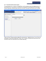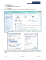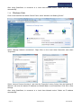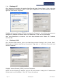
Download SmartSoft v3.1 User Manual

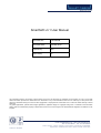
SmartSoft v3.1 User Manual
Document Ref:
3100-3008-B
Document Date:
24th May 2013
Prepared by:
KMJ
Approved by:
RT
This information herein is the property of Smart Fibres Ltd and is to be held strictly in confidence by the recipient. No copy is to be made
without the written permission of Smart Fibres Ltd. Disclosures of any of the information herein is to be made only to such persons who
need such information during the course of their engagement or employment at Smart Fibres Ltd or under the written authority of Smart
Fibres Ltd.
Any patent applications, patents and/or design applications, registered designs or copyrights arising from or contained in the information
herein, shall be considered the property of Smart Fibres Ltd and as such are subject to the aforementioned obligation of confidence on the
recipient.
Smart Fibres Ltd · Brants Bridge · Bracknell · RG12 9BG · United Kingdom
Email: [email protected] · Web: www.smartfibres.com
Tel: +44 1344 484111 · Fax: +44 1344 486759
Directors: C Staveley · A Melrose · Registered in England: 3563533 · VAT Registration No: GB723426060
Registered Office: 141 Dedworth Road · Windsor · Berkshire · SL4 5BB · United Kingdom
Certificate No: LRQ 4003532
1 Installation........................................................................................................................ 5
2 Preparing for use ............................................................................................................. 5
3 Basic Acquisition.............................................................................................................. 7
3.1 Basic acquisition – spectrum tab ............................................................................... 7
3.2 Basic acquisition – sensors tab ................................................................................. 8
3.3 Basic acquisition – charts tab.................................................................................... 9
4 Instrument Set-up .......................................................................................................... 10
4.1 Instrument set-up - acquisition rate tab ................................................................... 10
4.2 Instrument set-up - gain slots tab ............................................................................ 11
4.3 Instrument set-up - peak detection tab .................................................................... 13
4.4 Instrument set-up - network tab............................................................................... 14
4.5 Instrument set-up - load and save tab ..................................................................... 15
4.6 Instrument set-up - exiting instrument set-up .......................................................... 15
5 Enhanced Acquisition .................................................................................................... 16
5.1 Enhanced acquisition - spectrum tab ...................................................................... 16
5.2 Enhanced acquisition - select sensors tab .............................................................. 17
5.3 Enhanced acquisition - charts tab ........................................................................... 22
5.4 Enhanced acquisition - graphic tab ......................................................................... 23
5.5 Enhanced acquisition – plug-ins tab........................................................................ 24
5.6 Enhanced acquisition - exit data acquisition............................................................ 24
6 Plug-ins.......................................................................................................................... 25
6.1 Plug-In for FFT ........................................................................................................ 25
6.2 Plug-In for Network Time Protocol (NTP) synchronisation ...................................... 25
6.3 Plug-In For Software update ................................................................................... 27
7 Appendices .................................................................................................................... 28
7.1 IP address settings of Host PC................................................................................ 28
7.1.1 Windows 7 ........................................................................................................ 28
7.1.2 Windows Vista .................................................................................................. 29
7.1.3 Windows XP ..................................................................................................... 30
7.1.4 Windows 2000 .................................................................................................. 30
7.2 Diagnostic Output.................................................................................................... 31
7.3 Configuration of time of flight correction .................................................................. 31
Page 2
24th May 2013
3100-3008-B
Document Revision History:
Issue
B
A
Page 3
Issue Date
24th May 2013
14th June 2012
24th May 2013
Change
Clarified Acquisition rate setting
Copied 3100-3002-D, removed
hardware specific sections and
updated screen-shots and text for
SmartSoft v3.1
3100-3008-B
1
INSTALLATION
SmartScan is shipped with a CD containing installer files for the SmartSoft interface. The host PC
must run a suitable Operating System, this manual covers installation on a PC running Windows
2000, XP, Vista or 7. Installers for Linux and other operating systems may be available on request.
To install the software on the host PC navigate to “setup.exe” on the CD and follow the instructions
that appear during the install process. The installer will also install National Instruments’
LabVIEW TM Run Time Engine (RTE). It will then place a short cut in the Windows Start Menu
(under the Smart Fibres program group) and on the Desktop.
The latest release of SmartSoft can also be downloaded from the Smart Fibres website. Contact
Smart Fibres technical support for details.
2
PREPARING FOR USE
After installing SmartSoft, connect the supplied Ethernet cross-over cable between the host PC
and SmartScan. The PC’s network connection must be configured to a suitable subnet; by default
SmartScan’s IP address is 10.0.0.150 and its Net mask is 255.255.255.0. The Net mask for the PC
must also be set to 255.255.255.0, suitable ranges for the PC’s IP address are 10.0.0.1 to
10.0.0.149 or to 10.0.0.151 to 10.0.0.250. (see appendix 6.3 for further details or contact your
network administrator for assistance).
Connect the Power adaptor to the main AC supply and connect its DC output to the DC input of
SmartScan. Alternatively SmartScan can be powered directly from a DC supply, in which case the
DC supply must be in the range +9 to +36V and capable of supplying 15W of power and a DC
power cable should have been ordered with the SmartScan.
SmartScan is now ready to be powered. Switch on the supply and observe the Power/Status light
next to the DC power connector, it should first light red to indicate the presence of supply voltage
and then change to green after a few seconds to indicate that the SmartScan is ready for a host
PC connection. FBG sensors can be connected to the SmartScan at any time.
On the host PC Navigate to the Smart Fibres > SmartSoft short-cut on the Windows Start Menu
and start the program.
The program requests the IP address of the SmartScan. As shipped from the factory this will be
10.0.0.150. An Ethernet connection is attempted and the dialogue box changes to indicate
progress. If a connection can be made successfully the dialogue box will close after a few seconds
and the SmartSoft main screen appears.
Page 4
24th May 2013
3100-3008-B
Illustration 1: Front panel
A number of function buttons are shown top right. Inactive functions are greyed out.
Basic Acquisition is recommended for first time users and is designed to enable basic
measurements to be taken with simplified settings. Acquisition will be fixed at 2.5kHz (250Hz for
SmartScan lite), with per channel auto-gain. The data processing rate can be varied by averaging
a user defined number of samples (1-1000).
Enhanced Acquisition is recommended for advanced users and is rich in features but requires
more detailed settings. Attempting to use enhanced mode without first reading this manual is not
recommended.
Instrument Set-up is largely used in conjunction with Enhanced Acquisition.
Plug-ins allows the user to run custom LabVIEW source code modules. Contact Smart Fibres
technical support for details.
Quit is used to close the entire application. Always use the Quit button to exit the SmartSoft
application; using other methods to close the application may cause unexpected behaviour.
Page 5
24th May 2013
3100-3008-B
BASIC ACQUISITION
3
Press the Basic Acquisition Button and then select the Spectrum Tab.
3.1
BASIC ACQUISITION – SPECTRUM TAB
Illustration 2: Basic acquisition – Spectrum tab
The spectrum tab is intended as a tool to aid setting up of sensors and/or SmartScan parameters.
The sensors on one channel at a time can be viewed with the reflected signal intensity displayed
over the wavelength range. Each peak represents the reflected light from one FBG. In basic
Acquisition mode the gain is applied on a per channel basis. Automatic gain control ensures that
the largest signal is not saturated.
If there are large differences in the signal intensity of FBGs on the same channel then per FBG
gain can be used with the enhanced acquisition panel, see the Instrument Set Up section for more
details. Step through all the channels that have FBGs connected and ensure that the background
noise is below 10% and that the FBG signal peaks are above 25%.
If desired the instantaneous spectrum can be saved to file, press the save button whilst the
channel of interest is being viewed.
Next move to the Sensors tab.
3.2
BASIC ACQUISITION – SENSORS TAB
Page 6
24th May 2013
3100-3008-B
Illustration 3: Basic acquisition - Sensors tab
All FBG locations are shown in the table on the left of the screen. The number of FBGs per
channel can be programmed using Instrument Set Up.
The SmartScan calculates the centre wavelength of each FBG peak and these are displayed in
the table.
The user may record the table wavelengths to a log file. First set the target location and name of
the log file by typing it in the box, or by clicking the folder icon. Then set the duration of the logging
period (log time) and then press the log button. The button lights up and the elapsed time is
indicated by a progress bar and a numeric indicator. The recording will automatically stop when
the Log time is reached or the user may stop the recording by pressing the Log button again.
A log file can be scheduled to take place at regular intervals. The file name will be appended with
a date/time string of the format “YYYYMMDD-HHMM_” where YYYY is the year, MM is the month,
DD is the day, HH is the hour of day and MM is the minutes in the hour.
The number of lines per log file and the time/date format to append or prepend to the file-name
may be set by clicking the icon next to the “Log FBGs” heading.
Now move on to the Charts tab.
Page 7
24th May 2013
3100-3008-B
3.3
BASIC ACQUISITION – CHARTS TAB
Two wavelength graphs are displayed simultaneously and any of the available FBGs (16 per
channel) can be selected for display. FBGs can be added to the left or right y-axes and each one
is assigned a colour-coded trace.
To increase the displayed graph area one or both of the y-axes can be hidden by pressing the
appropriate < or > button. Similarly the lower graph can be hidden using the “V” button between
the two graphs, allowing the upper graph to extend to fill the screen.
Illustration 4: Basic acquisition – Charts tab
The Y axes of the graphs are set to auto-scale. If required, they can be locked by right clicking on
the desired axis and de-selecting “AutoScale Y”. The upper and lower limits of the locked axis can
then be selected and adjusted.
To finish the Acquisition session press Exit Data Acquisition or choose another panel from the
main controls.
Having mastered the Basic Acquisition the user may now explore the Enhanced Acquisition and
associated Instrument Set Up tabs. Alternatively, to close the entire SmartScan suite, press the
Quit button.
Page 8
24th May 2013
3100-3008-B
INSTRUMENT SET-UP
4
Instrument Set Up is used to enable Enhanced Acquisition and allows the powerful features of
SmartScan and SmartSoft to be utilised fully.
A number of set up tabs are available, they will be described from left to right.
4.1
INSTRUMENT SET-UP - ACQUISITION RATE TAB
Illustration 5: Setup - Acquisition rate tab
Here the user can adjust various parameters that affect the acquisition rate of the SmartScan and
the data processing rate of the SmartSoft software.
The lower half of the screen shows spectra from all operational channels, together with the current
wavelengths of any detected FBG peaks.
Starting on the left the user may configure the number of active optical channels. The limit
depends on the maximum number of optical channels the instrument supports.
The user may configure the number of FBGs per channel. Reducing the number of FBGs per
channel enables the faster acquisition rates in the drop down menu to be used.
The SmartScan cycle time in microseconds (µs) can be adjusted. The cycle time is defined as the
time to complete one laser tuning step and measure the light received by the detector circuits. This
can speed up or slow down the overall acquisition time. The minimum cycle time is 1 µs.
Page 9
24th May 2013
3100-3008-B
The SmartScan’s acquisition rate is a function of cycle time and wavelength range. The acquisition
rate can be adjusted by choosing a value from the selection box. This trades the instruments
wavelength range for acquisition speed, e.g. 2.5 kHz over 40 nm, 5 kHz over 20 nm, 25 kHz over 4
nm. For some rates it may be necessary to reduce the number of FBGs per channel as described
above.
Illustration 6: Setup - Acquisition rate selection
The active laser range will be reduced according to the selected acquisition rate. The inactive
range will be greyed out in the graph. Left click with the mouse to centre the active region in the
desired location. Select the lowest acquisition rate in the list to reset the active region to it's full
range.
Consideration should be given to the expected wavelength excursions of each FBG peak to
ensure that they will not move outside the laser tuning range.
The rate at which data are transmitted to the host PC can be reduced by sampling the data.
Setting the Data Rate to 1 means that the SmartScan will transmit all available data to the PC and
the transmission rate will be equal to the acquisition rate. Setting the Data Rate to a number N
greater than 1 will result in data from every Nth scan being transmitted. It may be desirable to slow
down the transmission rate because, for example the data are transmitted over a slow network
connection or because the host PC cannot process the data packets fast enough.
Finally the user may further reduce the amount of data stored in a log file by applying averaging or
decimating the data. This is applied by the SmartSoft application so will not reduce the Ethernet
traffic but will reduce the data presented by SmartSoft and optionally saved to file. The extent of
data reduction is controlled by the Sample size box. Setting this to a number n will result in every
nth transmitted data point being presented or stored, either by averaging n points together or by
keeping every nth point and discarding the rest. Averaging n data points together will also improve
the signal to noise ratio by up to a factor of √n.
The data processing rate is displayed at the top of the screen when acquisition is in progress. The
acquisition and transmission rates are shown as a tool tip when hovering the mouse over the data
processing rate indicator.
Page 10
24th May 2013
3100-3008-B
4.2
INSTRUMENT SET-UP - GAIN SLOTS TAB
Illustration 7: Setup - Gain slots tab
An advantage of Enhanced Acquisition is that it enables the use of Wavelength Gain slots,
whereby each FBG operates within its own wavelength window that is assigned its own set of
properties. Each slot can use a different gain level so large variations in signal intensity can be
accommodated on one channel without loss of measurement resolution.
The Gain slots are set up on a channel-by-channel basis. The spectrum for the Channel in
question is displayed. The wavelength limits on the graph's x-axis have already been determined
according to the laser tuning range that was set up on the Acquisition Rate tab. The user then
clicks between the spectral peaks to add slot boundaries. Only one FBG peak should be present in
each slot. The start and end points of the wavelength tuning range are slot boundaries, so be sure
not to add slot boundaries before the first FBG or after the last FBG. Care should be taken that
during operation the FBG peak will not cross a slot boundary and that FBG peaks remain
separated by at least 1.6 nm from each other and 0.8 nm from the end of the active laser range.
Do not set up more slots than the number of sensors per channel that was configured on the
Acquisition Rate tab.
Slot boundaries can be adjusted by dragging them to their desired position using the mouse. Right
click on a boundary to delete it.
Once the slots are established the Gain Mode can be set. There are two modes, in auto mode the
gain for each slot adjusts automatically so that the intensity of each FBG peak is maximised but
does not saturate. The peak intensity will be maintained between 50 and 100 % and will only
reduce below 50% on the highest gain level if the signal is still too small.
Page 11
24th May 2013
3100-3008-B
In Manual gain mode a fixed gain is applied to each slot. To set the gain, right click on the graph
between the slot boundaries and set the gain level between 0 and 8, repeating this process for
each slot on all channels. The optimum gain level is above 50% but without saturating; a saturated
FBG peak will have a flat top at around 100% intensity. The gain applied to each slot is displayed
on the graph. Selecting a manual gain for a slot will automatically change the gain setting from
auto to manual.
It is recommended that in manual mode the gain be set as high as possible without risk of the FBG
peak saturating. Peaks below 25% relative intensity may suffer reduced measurement
performance.
Page 12
24th May 2013
3100-3008-B
4.3
INSTRUMENT SET-UP - PEAK DETECTION TAB
Illustration 8: Setup - Peak detection tab
The peak detection threshold may be adjusted for each channel on this tab. Ensure the threshold
level is above the background reflection level but not above any true FBG peaks. In most cases a
value of around 15% is optimal.
SmartScan performs a baseline calibration of the photo-detectors during power up. This
compensates for any back-reflection in the fibres. The calibrated baseline value is shown as a red
trace on the graph. If the fibres are changed or disturbed and the baseline changes, calibration
can be performed by either power-cycling the instrument or pressing the “Calibrate baseline”
button.
The “ToF correction” button enables the correction of the detected wavelength by taking account
of the time of propagation through the optical fibre. This feature is mainly useful for optical fibre
longer than 100m. Before using this feature, the software should be configured with the Tof setup
plug-in described later.
Page 13
24th May 2013
3100-3008-B
4.4
INSTRUMENT SET-UP - NETWORK TAB
Illustration 9: Setup - Network tab
On the Network tab the user can change the IP settings of the SmartScan. This is usually only
necessary when a SmartScan is to be used on a Local Area Network. Be aware that the IP
settings of the host PC may need to change in order to maintain connectivity.
If you are connecting the SmartScan to a network instead of a direct connection to a host PC,
make sure to set the gateway address to match the network router or gateway PC's LAN address
and that the SmartScan's IP address is unique on the network and not in the pool of addresses
assigned to any DHCP servers on the network.
If there is a firewall or NAT router between the SmartScan and the host PC you may need to open
UDP ports 30001 to 30003, 30070 to 30072 and 30075 to allow SmartSoft to communicate with
the interrogator.
See Preparing For Use section and Appendix 6.3 for further details and if necessary consult your
Network Administrator.
Page 14
24th May 2013
3100-3008-B
4.5
INSTRUMENT SET-UP - LOAD AND SAVE TAB
Illustration 10: Setup - Load and save tab
The user can use this tab to save all the Instrument Setup parameters to a file. The file can be
recalled later using the Load button. This is particularly useful when SmartScan is used to
interrogate multiple sensor systems, as a configuration for each system can be saved.
4.6
INSTRUMENT SET-UP - EXITING INSTRUMENT SET-UP
There are three options for exiting Instrument Set Up, pressing “Save changes and exit” will
transfer all parameters to SmartScan and the instrument is ready to begin an Acquisition session.
Alternatively, pressing “Cancel changes and Exit” will discard any changes and SmartScan will
revert to its previous configuration. You can also just select a new panel from the main controls, if
any settings have been changed SmartSoft will ask if you want to save them.
Page 15
24th May 2013
3100-3008-B
ENHANCED ACQUISITION
5
Before entering Enhanced Acquisition first go to the Instrument Set Up section.
5.1
ENHANCED ACQUISITION - SPECTRUM TAB
Illustration 11: Enhanced – Spectrum tab
The spectrum tab is intended as a tool to aid setting up of sensors and/or SmartScan parameters.
The sensors on one channel at a time can be viewed with the reflected signal intensity displayed
over the wavelength range. Each peak represents the reflected light from one FBG. The
appearance of the FBG Peaks will be influenced by the Gain scheme selected during Instrument
Set Up.
If desired the instantaneous spectrum can be saved to file, press the save button whilst the
channel of interest is being viewed. An image of the spectrum can be exported to the clipboard or
a file by right clicking in the graph area.
Note that the data rate for spectral data is much slower than for sensor data
The graph palette in the top left corner of the graph provides options for navigating around the
screen. The cross icon is the selection tool and is used for selecting and moving graph cursors,
the magnifying glass icon allows the user to zoom in on the graph to examine particular spectral
features in more detail and the hand icon is used to drag a magnified region around the plot.
The plot legend in the top right of the graph can used to change the plot properties, e.g. line
style/colour, point style/colour, etc.
Page 16
24th May 2013
3100-3008-B
Extra functionality is made available by right clicking in the graph and selecting from the pop-up
menu. The scale legend can be used to gain quick access to the graphs auto-scale options and for
changing scale indicator parameters such as numeric format, precision, etc. The cursor legend is
used for creating cursors on the graph and reading the position of those cursors. Cursors can be
created by right clicking inside the cursor legend and can be dragged with the selection tool (see
graph palette section). The cursor can be configured by right clicking on it's name in the cursor list.
5.2
ENHANCED ACQUISITION - SELECT SENSORS TAB
Illustration 12: Enhanced acquisition – Sensors tab
The Select Sensors tab has two tables. The left hand table displays all available FBGs, the
number being determined during the Instrument Set Up by the Sensors per Channel setting and
the number of gain slots. If there are more FBG Peaks on the Spectrum tab than available FBGs in
the table then revisit the Instrument Set Up and either add more Gain Slots or increase the
Sensors per channel setting. If a gain slot is set up without an FBG reflection within it, a sensor
wavelength of zero is returned in the table.
The FBG table displays all the FBGs on channel 1 in descending wavelength order followed by
those on channel 2 and so on. The channels are colour coded for ease of identification. For each
FBG there are columns for its current wavelength as well as average, minimum and maximum.
The right hand table displays the selected Sensors; this table will be empty to start with. Sensors
are added to the table using the “ADD...” button or by right clicking on a grating in the FBG table.
This brings up the add sensor dialogue box.
Page 17
24th May 2013
3100-3008-B
Illustration 13: Sensor dialog box - Sensor type page
The user can select one of the FBGs from a drop down list of all available FBGs. The user may
now give the sensor a meaningful name and change the measurement units. In the case of a
wavelength sensor (as shown above), there is only one page to fill out and once a sensor name
has been entered the OK button will become active.
For measurements other than Wavelength the user must enter a number of parameters so that
SmartSoft can make the conversion. The next button will become active allowing the definition of
multiple gratings, sensors and coefficients as determined by the sensor type. Selecting a strain
sensor type and clicking next leads to the following dialog box page.
Illustration 14: Sensor dialog box - Gratings page
Page 18
24th May 2013
3100-3008-B
The reference wavelength is the wavelength against which the grating will be compared. For some
sensor types, SmartSoft needs to measure a change in the wavelength of an FBG in order to
convert to engineering units such as strain, temperature and pressure. The reference wavelength
may be supplied by the sensor manufacturer or it can be entered by selecting one or more
gratings, choosing the mean, minimum, maximum or current value in the reference wavelength
selection box and pressing the blue arrow button to update al selected gratings. It may be
necessary to set the type to wavelength and then log and analyse some data in order to determine
the required reference wavelength. The grating selection page will not be available if the sensor
type selected does not require it.
Press next to advance to the next dialog box page.
Illustration 15: Sensor dialog box - Sensors page
A sensor can use the values of other, previously defined sensors. In the case of a strain sensor, a
temperature sensor can be selected to perform temperature compensation. Temperature sensors
must be defined before they are available for use. Notice that the sensor name refers to
temperature change. The temperature sensor must be configured to show relative rather than
absolute temperature (i.e. relative to the temperature at the reference wavelength).
The types of sensors available to choose from is determined by the sensor type selected. The
sensor selection page will not be available if the sensor type selected does not require it.
Press next to advance to the next dialog box page.
Page 19
24th May 2013
3100-3008-B
Illustration 16: Sensor dialog box - Coefficients page
If the sensor requires constant coefficients, enter them here. They should be provided with the
sensor.
The type of conversion coefficients requested by the sensor set-up dialogue box is determined by
the sensor type selected. The coefficient selection page will not be available if the sensor type
selected does not require it.
If all required information has been entered the OK button should become active. Press OK to
save the sensor. Press cancel at any time to exit the dialog box.
When the Add sensor dialogue box is closed the new sensor will now appear in the sensor table.
Further FBGs can then be selected to add more sensors to the table and the Sensor order can be
adjusted using the “UP” and “DOWN” buttons. Sensor parameters can be amended using the
“EDIT” button.
When the sensor table is complete press the “SAVE...” button so that the sensor parameters can
be re-loaded during future acquisition sessions. Multiple Sensor selections can be saved with
different file-names. SmartSoft loads the last used sensor set-up when starting the enhanced
acquisition panel. If gratings have been removed or changed you can change the sensor set-up
with the “DELETE” and “EDIT...” buttons.
The logging feature on this tab can be used to save all the sensors present in the Sensor table.
Sensors will be logged at the Data Processing Rate displayed at the top of the screen.
Set the target location and name of the log file by typing it in the box, or by clicking the folder icon.
Then set the duration of the logging period (log time) and then press the log button. The button
lights up and the elapsed time is indicated by a progress bar and a numeric indicator. The
recording will automatically stop when the Log time is reached or the user may stop the recording
by pressing the Log button again.
Page 20
24th May 2013
3100-3008-B
The number of lines per log file and the time/date format to append or prepend to the file-name
may be set by clicking the icon next to the “Log sensors” heading.
A log file can be scheduled to take place at regular intervals. The file name will be appended with
a date/time string of the format “YYYYMMDD-HHMM_” where YYYY is the year, MM is the month,
DD is the day, HH is the hour of day and MM is the minutes in the hour.
Data is saved in tab separated format suitable for opening with common spreadsheet applications
such as Microsoft Excel and OpenOffice Calc.
The Start Time is given in standard UTC format, which is the number of seconds since 00:00 on 1st
January 1970.
Illustration 17: Example log file
5.3
ENHANCED ACQUISITION - CHARTS TAB
Page 21
24th May 2013
3100-3008-B
Illustration 18: Enhanced acquisition – Charts tab
By default two charts are shown, each with dual y-axes. All the Sensors present in the Sensor
table are available for adding to the charts, this is achieved by selecting the tick box next to each
sensor.
The left and right y-axes of each chart can be set to different measurement units. The chart can be
expanded by hiding one of the y-axes using the appropriate “X” button. The entire lower chart can
also be hidden by pressing the “V” button, whereby the upper chart expands to fill the whole tab.
The y-axes of the charts auto-scale by default but by right clicking on the charts the user may
disable auto-scaling and may then edit the maximum and minimum y-axis limits to display the
desired amplitude range.
An image of the chart can be exported to the clipboard or saved to a file by right clicking on the
graph and selecting “Export simplified image...”.
Page 22
24th May 2013
3100-3008-B
5.4
ENHANCED ACQUISITION - GRAPHIC TAB
Illustration 19: Enhanced acquisition - Graphic tab
On the graphic tab the user may load a photograph or diagram of the structure being monitored.
The file must be in JPG format and 800 x 600 pixels. Some example pictures are installed with the
application and are located in the common application data directory e.g. “C:\Documents and
Settings\All Users\Application Data\Smart Fibres\SmartSoft SSI\Graphics”. The location of the
common application data folder is dependant on your version of Windows, the example shown is
for Windows XP.
By right clicking on the graphic the user may add sensors from the sensor table and display their
current values in numeric or mini-graph form. By right clicking on an existing sensor it may be
deleted or modified in type.
Page 23
24th May 2013
3100-3008-B
5.5
ENHANCED ACQUISITION – PLUG-INS TAB
Illustration 20: Enhanced acquisition - Plug-ins tab
The plug-ins tab is used for running LabVIEW source code, these can be written by the end user
to increase and customise the functionality of the SmartSoft user interface. SmartSoft may be
supplied with a variety of plug-ins, including one for performing FFT analysis on a selected grating.
Details on how to write plug-ins can be obtained on request from Smart Fibres.
5.6
ENHANCED ACQUISITION - EXIT DATA ACQUISITION
Press “Exit Data Acquisition” to leave this area of the application.
Page 24
24th May 2013
3100-3008-B
6 PLUG-INS
6.1
PLUG-IN FOR FFT
A Fast Fourier Transform (FFT) of live wavelength data can be viewed allowing the user to
observe the frequency content of signals. Each FBG can be viewed on the graph using the “FFT
Grating” drop-down menu. By selecting the Magnifying glass icon the user may zoom in to view a
particular area of the frequency spectrum, select the cross-hair icon zoom out again. The
frequency scale on the x-axis will be determined by the Acquisition frequency. FFT theory dictates
that the frequency scale will be half the sample frequency. The sample frequency is the
transmission rate as set up during Instrument Set Up and can be viewed by hovering the mouse
over the Data Processing value at the top of the screen.
6.2
PLUG-IN FOR NETWORK TIME PROTOCOL (NTP) SYNCHRONISATION
The embedded Linux versions of SmartScan can either synchronise their time with the
host PC, which is performed when SmartSoft is launched, or it can connect to one or more
NTP servers. Note to use NTP ensure that the SmartScan can access the NTP server,
unless the NTP server resides on the host PC this will usually mean that the SmartScan
must have a connection to the internet or a local area network. To configure the time
source run the Plug-ins panel and select the NTP settings plug-in.
The list box will be populated with a list of NTP servers that the SmartScan is currently
configured to query. The NTP sync button shows the current time sync mode (ON = NTP,
OFF = SmartSoft host PC). From here you can add and delete servers and enable and
Page 25
24th May 2013
3100-3008-B
disable NTP. Press “Save&Exit” when done to configure the SmartScan or “Exit” to exit
without changing the SmartScan's settings. The “Add...” button launches a server
configuration dialog box.
The options are described in the ntpd documentation available at
http://support.ntp.org/bin/view/Main/WebHome and are briefly described below.
Server – IP address of the NTP server. Most NTP servers are known by their DNS name, to
discover the IP address of an NTP server use one of the many DNS Look Up websites or run:
ping your_ntp_server_name from the windows command prompt.
Prefer - Marks the server as preferred. All other things being equal, this host will be chosen for
synchronization among a set of correctly operating hosts. Only one server should have this set.
Burst - when the server is reachable, send a burst of eight packets instead of the usual one. The
packet spacing is 2 s. This is designed to improve timekeeping quality but may not be
appreciated by the NTP server’s owner.
Iburst - When the server is unreachable, send a burst of eight packets instead of the usual
one. The packet spacing is 2 s. This is designed to speed the initial synchronization
acquisition.
Min/Max poll - These options specify the minimum and maximum poll intervals for NTP
messages, as a power of 2 in seconds The maximum poll interval defaults to 10 (1,024 s),
but can be increased by the maxpoll option to an upper limit of 17 (36.4 h). The minimum
poll interval defaults to 6 (64 s), but can be decreased by the minpoll option to a lower limit
of 4 (16 s).
Version - Specifies the version number to be used for outgoing NTP packets. Valid values
are 1-4, the default and recommended value is version 4.
Page 26
24th May 2013
3100-3008-B
6.3
PLUG-IN FOR SOFTWARE UPDATE
The embedded Linux versions of SmartScan can be updated using the Update plug-in. If
the SmartScan is connected to a LAN that is accessible via the Internet then this makes
remote upgrades possible without having to visit the site where the instrument is located.
Select a Smart Fibres provided update file and press the “Update” button. You will then be
prompted to reboot the SmartScan. Press “Yes” to reboot. SmartSoft will disconnect and
reconnect when the SmartScan has finished rebooting.
Page 27
24th May 2013
3100-3008-B
7 APPENDICES
7.1
IP ADDRESS SETTINGS OF HOST PC
7.1.1
Windows 7
Click on the Start Bar and select Control Panel, select “Network and Sharing Centre”.
Select “Change adapter settings”, Right Click on the Local Area Connection and select
“Properties”
Select “Internet Protocol Version 4” and click the “Properties” button. Select “Use the following IP
address” and enter the desired IP address and Subnet Mask to suit SmartScan. Click OK to save
settings.
Page 28
24th May 2013
3100-3008-B
After using SmartScan, to reconnect to a Local Area Network select “Obtain an IP address
automatically”.
7.1.2
Windows Vista
Click on the Start Bar and select Control Panel, select “Network and Sharing Centre”.
Select “Manage Network connections”, Right Click on the Local Area Connection and select
“Properties”
Select “Internet Protocol Version 4” and click the “Properties” button. Select “Use the following IP
address” and enter the desired IP address and Subnet Mask to suit SmartScan. Click OK to save
settings.
After using SmartScan, to reconnect to a Local Area Network select “Obtain an IP address
automatically”.
Page 29
24th May 2013
3100-3008-B
7.1.3
Windows XP
On a Windows XP machine, click and the Start Bar and select “Control Panel.” Click on the icon
entitled “Network Connections” to open. When open, highlight the “Local Area Network” selection,
right click, and choose “Properties”.
Highlight the “Internet Protocol (TCP/IP)” entry and click “Properties”. You will then have access to
change the IP address and Subnet mask to suit SmartScan. Click “OK” to save settings.
After using SmartScan, to reconnect to a Local Area Network select “Obtain an IP address
automatically”.
7.1.4
Windows 2000
On a Windows 2000 machine, click on the Start Bar and select “Settings”, then “Control Panel”.
Double-click on “Network and Dial-up Connections”. Right click on “Local Area Connection” and
choose “Properties”.
Highlight “Internet Protocol(TCP/IP)” and click “Properties”.
Select “Use the following IP address” and you will have access to change the IP address and
Subnet mask to suit SmartScan. Click “OK” to save the settings.
Page 30
24th May 2013
3100-3008-B
After using SmartScan, to reconnect to a Local Area Network select “Obtain an IP address
automatically”.
7.2
DIAGNOSTIC OUTPUT
The serial port communicates various diagnostic parameters via RS232. It is primarily
used by Smart Fibres service personnel and should not be used by the user unless guided
to do so by a Smart Fibres engineer.
7.3
CONFIGURATION OF TIME OF FLIGHT CORRECTION
In order to configure correctly the time of flight correction, a plug-in called “tof setup plugin”, needs to be executed. The plug-ins tab can be activated by pressing the “Plug-ins”
button located top-right of the SmartSoft Interface, then the “tof setup plug-ins” can be
selected from list on the left of the main screen as shown in the picture below.
To create a new time of flight profile you need to follow this procedure:
1) Click “create new config file”
2) Write a file name into the box “New file name”, for example “delay line test”
3) Fill the boxes in the Distance (m) table with the distance of each sensor from the
SmartScan in metres. The table has one line per fibre channel and the distance of FBG
should be added starting from the left. See on example in the following picture.
4) When all distances have been entered click on the OK button.
5) The other two tables on the ToF tab are usually for indication only and do not need to
be filled in unless instructed by a Smart Fibres technician.
Page 31
24th May 2013
3100-3008-B
On this example, the first grating on Channel 2 is located at 1001m from the SmartScan,
the second grating at 1002m, the third at 1003m and the fourth at 1004m. Then, once the
procedure over, you can see your new tof configuration file name on the dropping list.
Later, if you want to use a previous existing file, you have just to select the file you want to
use and to click “Select config file to use”.
Smart Fibres may provide a pre-written ToF config file, which can be loaded in this way.
Page 32
24th May 2013
3100-3008-B