Download Calibrating the microStar

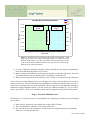
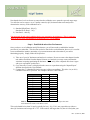
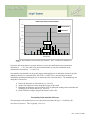
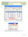
Calibrating the microStar
Clifford J. Yahnke, Ph.D.
Director of Technology
Before you begin making measurements the microStar should be calibrated to your specific environment.
This process, (i.e. creating a calibration curve) is extremely important as it correlates the optical response
from a dosimeter to a known dose in order to establish the sensitivity of the system (measured in
counts/dose). Fortunately, this is simple to do and the results can be stored for later use. The process has
the following steps:
1)
2)
3)
4)
5)
6)
7)
8)
Connect the Reader
Determine the Operating Environment
Determine the Calibration Type
Select the Calibration Dosimeters
Expose the Calibration Dosimeters
Establish the microStar Performance
Build the Calibration Curve
Test the Calibration Curve
Step 1 - Connect the Reader
Connect the microStar to the laptop, turn on the power and start the microStar software application. Wait
10 min. for the device to warm up and enter the “Configuration” tab as shown in the user’s manual.
Step 2 - Determine the Operating Environment
The microStar is designed to analyze dosimeters made from Al2O3:C. As shown in Figure 1 below, this
dosimetry material over-responds to diagnostic x-rays by a factor of ~3-4 as compared to higher-energy
gamma rays (e.g. Cs-137 and Co-60) and oncology linear accelerators (6MV+ photons/electrons).
Therefore a separate calibration curve is needed for each application. Fortunately, the microStar can be
calibrated to any set of operating conditions and the corresponding calibration curve can be stored within
the reader for later use.
Energy Response of Al2O3:C with Photon Energy (keV)
3.50
Response Relative to Cs-137
3.00
2.50
2.00
1.50
1.00
0.50
0.00
0
100
200
300
400
500
600
700
Energy (keV)
Figure 1. The difference in the energy response of Al2O3:C between diagnostic
x-rays and high-energy photons. Note the “flat” range at 662+ keV for radiation
oncology.
At this point, you simply need to determine if the calibration curve that you wish to create will be for:
A)
Diagnostic radiology
Or
B)
Radiation oncology
and proceed to the next section- Determine the Calibration Type. Note that there are two separate set of
instructions- one for diagnostic radiology and the other for radiation oncology.
Rev. 2, June 10, 2009
Calibrating the microStar (Diagnostic Radiology Users)
Step 3 - Determine the Calibration Type
For virtually all diagnostic radiology users, a linear calibration is sufficient to achieve the desired level of
accuracy (<10%). For those customers with special accuracy requirements, a non-linear calibration can
be used. Refer to the section for radiation oncology users to learn more about this feature.
Step 4 - Obtain the Calibration Dosimeters
Having chosen the application and the calibration type, you must next obtain a set of calibration
dosimeters. For diagnostic radiology customers, Landauer supplies a set of dosimeters exposed on a
PMMA phantom to 80 kVp x-rays (HVL = 2.9mm Al). These are supplied with the microStar when you
purchased it. Advanced users could create their own set using the technique outlined for radiation
oncology customers with the appropriate type of machine (fluoroscope, CT, mammograph)
Step 5 - Expose the Calibration Dosimeters
The calibration set supplied by Landauer will span the range of clinical applications for virtually all
diagnostic radiology users. Advanced users could create their own set using the technique outlined for
radiation oncology customers with the appropriate type of machine (fluoroscope, CT, mammograph).
Step 6 - Establish the microStar Performance
Using your set of calibration and QC dosimeters, you will next need to establish the intrinsic precision of
your microStar. This does not need to be done before each calibration; however, it is a useful test to
understand the intrinsic uncertainty of your measurements and to determine if your unit is functioning
properly. Simply follow the steps below:
1) Take a 100,000 mRad QC dosimeter (or a “high-dose” dosimeter if you created your own set) and
analyze it ten times. Be sure to remove the adapter from the unit and the dosimeter from the
adapter between each analysis to average out any mechanical variations in opening/positioning
the dosimeter. Don’t worry if the computed dose doesn’t agree with your expectations (at this
time).
2) Copy down the “Counts” as displayed on the screen or export them using the “Import/Export”
function described in the Users Manual.
3) Compute the CV (Standard Deviation/Average) of these ten readings. This is the 1-σ (or 68%)
confidence interval for your unit. An example is shown in Table 1 below.
Rev. 2, June 10, 2009
Dose
(mRem)
Counts
Reading 1
66715
4270
Reading 2
67105
4295
Reading 3
68761
4401
Reading 4
68674
4395
Reading 5
67895
4346
Reading 6
69142
4425
Reading 7
68507
4385
Reading 8
69408
4442
Reading 9
68442
4381
Reading 10
68666
4395
Standard Deviation
855.1
54.73
Average
68331.5
4373.5
CV
1.3%
1.3%
Table 1. Example of CV Test for a microStar. Note that the test gives the same
result whether the counts or the Dose is used.
This result should be less than 2% and is typically far less (~1%). If it is not, repeat this test with two
other QC dosimeters and average all 3 CV’s. If the result is still larger than 2%, then it is likely that your
adapter is not opening smoothly. Landauer Inc. has established a protocol that addresses this. Contact
your Landauer sales representative or [email protected] for assistance.
Step 7 - Build the Calibration Curve
Now that you have established the performance of the unit you will need to analyze the calibration
dosimeters in order to build the calibration curve. This curve consists of two segments, corresponding to
different dose levels.
The microStar uses a photomultiplier tube (PMT) to collect the luminescence from an OSL dosimeter. As
such, it has a finite range over which it can accurately quantify this luminescent signal. Doses at the
bottom end of the dynamic range require large amounts of stimulation to provide a response
distinguishable from background and noise while doses at the top end of the dynamic range produce an
optical response that can saturate the PMT. This is graphically shown in Figure 2 below.
Rev. 2, June 10, 2009
Counts
Error
120.0%
1.E+06
100.0%
1.E+04
1.E+03
1.E+02
Excess Error
1.E+05
60.0%
40.0%
20.0%
1.E+01
1.E+00
1.E+00
80.0%
1.E+01
1.E+02
1.E+03
1.E+04
1.E+05
1.E+06
Counting Error (%)
1.E+07
PMT Saturation
PMT Counts
PMT Linearity and Counting Error
0.0%
1.E+07
Dose (m Rad)
Figure 2. Graphic depiction of the dynamic range afforded by a generic
photomultiplier tube (PMT). The range is constrained by the counting error on
one end and by saturation of the device on the other.
At doses above 10,000 mRad, the luminescent signal is large enough that the amount of applied
stimulation can be reduced. This has the effect of extending the dynamic range of the unit to ~ 500,0001,500,000 mRad depending upon the operating environment (500,000 mRad for diagnostic x-rays and
1,500,000 mRad for oncology). The two levels of optical stimulation are referred to as “strong” (for
doses < 10,000 mRad) and “weak” (for doses > 10,000 mRad). These correspond to “low-“ and “highdoses” respectively. The terminology used, “low” and “high”, is only a relative term used to characterize
the amount of optical stimulation applied and is not indicative of an absolute dose. After all, a dose that is
high to a diagnostic radiologist would typically be thought of a very low by an oncologist. This is shown
graphically in Figure 3 below.
Rev. 2, June 10, 2009
microStar Dynamic Range Separation
Counts
Error
1.E+07
120.0%
"Low-Dose"
Region
1.E+06
"Cross-Over" Point
1.E+04
1.E+03
1.E+02
80.0%
60.0%
40.0%
20.0%
1.E+01
1.E+00
1.E+00
100.0%
Counting Error (%)
PMT Counts
1.E+05
"High-Dose"
Region
1.E+01
1.E+02
1.E+03
1.E+04
1.E+05
1.E+06
0.0%
1.E+07
Dose (mRad)
Figure 3. Definition of the two dynamic ranges used in the microStar. Each
range has its own level of optical stimulation designed to balance error and
depletion of the sample. The “dip” in the PMT counts between the two regions
is due to the different amounts of luminescence (per unit dose) created by the
different levels of optical simulation.
1) Go to the “Calibration” tab in the microStar software and click the radio button corresponding to
the desired calibration (High-Dose or Low-Dose).
2) Begin to analyze the dosimeters, entering their exposed dose in the upper right corner. Be sure to
read each dosimeter 3 times to obtain a total of 9 readings for each dose level.
3) When you have analyzed all of the dosimeters, click “Accept” to accept and store the calibration.
Once you have stored the calibration curve, you can apply one or more correction factors to it in order to
improve its accuracy. The correction factors are multiplicative constants and shift the entire curve up or
down and are not usable with a non-linear calibration. They are typically used in diagnostic radiology to
translate the supplied calibration (80 kVp, 2.9 mm Al HVL) to a different modality (e.g. CT @ 120 kVp
and 8.3 mm Al HVL). Their use is described in more detail in Appendix A at the end of this document.
Step 8 - Test the Calibration Curve
The final step is to verify the accuracy of the calibration curve using the QC dosimeters created during the
process above.
1) Read each QC dosimeter 4 times and take the average of the 12 results.
2) The average should be within 2% of the exposed dose level.
3) If it is not, then review the readings to see if the results for a single dosimeter are significantly
different (> 2%) than the other two.
Rev. 2, June 10, 2009
4) If this is the case, then disregard all data from this dot and re-compute the average of the other
two dots (8 readings). It is possible (< 5% chance) that during the screening process a dosimeter
will have an individual sensitivity different from its labeled value by more than 2%. This is
described in more detail in the section titled, Uncertainty in the Sensitivity of an Individual
Dosimeter the Using the microStar portion of this document.
5) If this is still not within 2% of the exposed dose level, then you will need to investigate your
calibration curve to see if there are any anomalous readings (defined as > 2% of the average for
that dose level).
Rev. 2, June 10, 2009
Calibrating the microStar (Radiation Oncology Users)
Step 3 - Determine the Calibration Type
Once you have selected the operating environment, you next need to decide upon the dynamic range (for
the dose) over which you wish to make measurements. The microStar uses a photomultiplier tube (PMT)
to collect the luminescence from an OSL dosimeter. As such, it has a finite range over which it can
accurately quantify this luminescent signal. Doses at the bottom end of the dynamic range require large
amounts of stimulation to provide a response distinguishable from background and noise while doses at
the top end of the dynamic range produce an optical response that can saturate the PMT. This is
graphically shown in Figure 2 below.
Counts
PMT Linearity and Counting Error
Error
1.E+07
120.0%
1.E+06
100.0%
Excess Error
1.E+03
80.0%
60.0%
40.0%
1.E+02
20.0%
1.E+01
1.E+00
1.E-03
Counting Error (% )
1.E+04
PMT Saturation
PMT Counts
1.E+05
1.E-02
1.E-01
1.E+00
1.E+01
1.E+02
1.E+03
0.0%
1.E+04
Dose (cGy)
Figure 2. Graphic depiction of the dynamic range afforded by a generic
photomultiplier tube (PMT). The range is constrained by the counting error on
one end and by saturation of the device on the other.
At doses above 10 cGy, the luminescent signal is large enough that the amount of applied stimulation can
be reduced. This has the effect of extending the dynamic range of the unit to ~ 500-1500 cGy depending
upon the operating environment (500 cGy for diagnostic x-rays and 1500 for oncology). The two levels
of optical stimulation are referred to as “strong” (for doses < 10 cGy) and “weak” (for doses > 10 cGy).
These correspond to “low-“ and “high-doses” respectively. The terminology used, “low” and “high”, is
only a relative term used to characterize the amount of optical stimulation applied and is not indicative of
an absolute dose. After all, a dose that is high to a diagnostic radiologist would typically be thought of a
very low by an oncologist. This is shown graphically in Figure 3 below.
Rev. 2, June 10, 2009
Counts
microStar Dynamic Range Separation
Error
1.E+07
1.E+06
30.0%
"Low-Dose"
Region
"High-Dose"
Region
"Cross-Over" Point
1.E+04
1.E+03
1.E+02
20.0%
15.0%
10.0%
5.0%
1.E+01
1.E+00
1.E-03
Counting Error (%)
PMT Counts
1.E+05
25.0%
1.E-02
1.E-01
1.E+00
1.E+01
1.E+02
1.E+03
0.0%
1.E+04
Dose (cGy)
Figure 3. Definition of the two dynamic ranges used in the microStar. Each
range has its own level of optical stimulation designed to balance error and
depletion of the sample. The “dip” in the PMT counts between the two regions
is due to the different amounts of luminescence (per unit dose) created by the
different levels of optical simulation.
A typical calibration curve has two segments for each of these dose ranges, however, for users who
desire very accurate measurements (~1-2%) at high doses (> 300 cGy), an alternative is provided. This
is necessary due to the non-linear response of the dosimetry material and PMT at these dose levels.
A non-linear calibration feature is available on the “Configuration” tab in the microStar software as
shown in the users manual. By “checking” the appropriate box in the lower left corner of the screen (and
“Saving”), the user will disable the standard calibration process and make available the non-linear
calibration option. The differences between this type of calibration and a standard calibration are:
• It is only usable for “high-doses” (i.e. > 10 cGy)
• It fits a second order polynomial of the form y = ax2 + bx + c to the calibration data to establish
the calibration curve. Note that without this option, the microStar fits a straight line to the
calibration data.
Therefore, the user will need to determine how they wish to calibrate the reader:
1) Standard (i.e. Linear) calibration
Or
Rev. 2, June 10, 2009
2) Non-linear calibration
Regardless of the type of calibration chosen, the user will need to create the dosimeters used to actually
build the curve as described in Step 5 - Expose the Calibration Dosimeters.
Step 4 - Obtain the Calibration Dosimeters
Having chosen the application and the calibration type, you must build a set of calibration and quality
control (QC) dosimeters. This is simple to do and requires the use of “screened” dosimeters from
Landauer. The effect and importance of using “screened” dosimeters is described in more detail under
the Using the microStar section later in this document. For now, just note that you need “screened”
dosimeters and be sure to specify this when purchasing the dosimeters from Landauer. This is strongly
recommended for all therapy users. Failure to use screened dosimeters can increase the uncertainty
associated with the calibration curve by up to a factor of 4.
Step 5 - Expose the Calibration Dosimeters
The calibration dosimeters are exposed to a set of conditions that you wish to establish as your reference.
Note that while the dosimetry material has an energy dependence between 80 kVp (diagnostic) and
therapy (6MV+), previous studies have shown that it has little to no dependence over the range of beams
found in an oncology clinic [Jursinic, P.A. Med. Phys. 34, 4594-4604 (2007)]. These same studies have
also shown it to have little to no angular, modality (photon/electron), dose rate, or temperature
dependence. Therefore, one can use a single calibration curve to represent most if not all of the
conditions encountered in a radiation therapy clinic.
Of course, one can achieve an even higher level of accuracy if separate calibration curves are made for
each beam. The microStar can easily accommodate this as it has the ability to store multiple calibration
curves for later use.
After selecting the beam type to be used (photon/electron and energy), the dosimeters are placed in a
water-equivalent scattering environment as shown in Figures 4(a)-4(c) below.
Rev. 2, June 10, 2009
Figures 4(a)-4(c). Upper left (a): Experimental setup showing solid water and the placement of
one (or more) nanoDots. Upper right (b): Flexible water placed over the dosimeter to remove air
gaps and ensure a tissue-equivalent scattering environment. This setup uses a 0.5 cm sheet to
achieve this. Bottom (c): Placement of solid water on top of the flexible to achieve the proper
depth. This setup uses a 1.0 cm sheet giving a total dosimeter depth of 1.5cm including the 0.5cm
from (b).
The bottom half of the picture depicts a semi-infinite scattering medium created from solid-water. The
thickness should be greater than D70% for the beam in question. This is typically 10 cm or more for 6MV.
Next, solid water is placed over the dosimeter to place it a Dmax. This is typically 1.5cm for 6MV. A
flexible slab is recommended to ensure that there are no air-gaps surrounding the dosimeter. Many users
elect to use 0.5cm of flexible water with 1cm of solid water directly above it.
The use of buildup is critical to ensure charged-particle equilibrium (CPE) and, more importantly, to
ensure that electron contamination from head-scattering of the machine or surface scattering from the
patient is eliminated.
The dosimeters are exposed in groups of 3 to a variety of dose levels depending upon the calibration type
chosen above:
1) Standard (High-Dose): 0, 50 cGy, 150 cGy, 300 cGy
Standard (Low-Dose): 0, 1 cGy, 5 cGy
2) Non-linear – 10 cGy, 100 cGy, 300 cGy, 500 cGy, 800 cGy, 1000 cGy, 1300 cGy
Rev. 2, June 10, 2009
Note that the dose levels are chosen to ensure that the calibration curve spans the expected usage range.
You will also need to expose a set of 3 quality control (or QC) dosimeters that can be analyzed to
determine the accuracy of the calibration curve:
1) Standard (High-Dose): 200 cGy
Standard (Low-Dose): 3 cGy
2) Non-linear – 600 cGy
You must wait 10 min. after irradiation before you can analyze the dosimeters. This is required to
allow for the low-level, non-dosimetric electron traps (~0.7 eV) to stabilize.
Step 6 - Establish the microStar Performance
Once you have a set of calibration and QC dosimeters, you will next need to establish the intrinsic
precision of your microStar. This does not need to be done before each calibration; however, it is a useful
test to understand the intrinsic uncertainty of your measurements and to determine if your unit is
functioning properly. Simply follow the steps below:
1) Take one of your QC dosimeters and analyze it ten times. Be sure to remove the adapter from the
unit and the dosimeter from the adapter between each analysis to average out any mechanical
variations in opening/positioning the dosimeter. Don’t worry if the computed dose doesn’t agree
with your expectations (at this time).
2) Copy down the “Counts” as displayed on the screen or export them using the “Import/Export”
function described in the Users Manual.
3) Compute the CV (Standard Deviation/Average) of these ten readings. This is the 1-σ (or 68%)
confidence interval for your unit. An example is shown in Table 2 below.
Counts Dose (cGy)
Reading 1
66715
76.0
Reading 2
67105
76.5
Reading 3
68761
78.4
Reading 4
68674
78.3
Reading 5
67895
77.4
Reading 6
69142
78.8
Reading 7
68507
78.1
Reading 8
69408
79.1
Reading 9
68442
78.0
Reading 10
68666
78.3
Standard Deviation
855.1
0.975
Average
68331.5
77.9
CV
1.3%
1.3%
Table 2. Example of CV Test for a microStar. Note that the test gives the same
result whether the counts or the Dose is used.
This result should be less than 2% and is typically far less (~1%). If it is not, repeat this test with two
other QC dosimeters and average all 3 CV’s. If the result is still larger than 2%, then it is likely that your
Rev. 2, June 10, 2009
adapter is not opening smoothly. Landauer Inc. has established a protocol that addresses this. Contact
your Landauer sales representative or [email protected] for assistance.
Step 7 - Build the Calibration Curve
Now that you have established the performance of the unit you will need to analyze the calibration
dosimeters in order to build the calibration curve.
1) Go to the “Calibration” tab in the microStar software and click the radio button corresponding to
the desired calibration (High-Dose, Low-Dose, or NL (for non-linear)).
2) Begin to analyze the dosimeters, entering their exposed dose in the upper right corner. Be sure to
read each dosimeter 3 times to obtain a total of 9 readings for each dose level.
3) When you have analyzed all of the dosimeters, click “Accept” to accept and store the calibration.
Once you have stored the calibration curve, you can apply one or more correction factors to it in order to
improve its accuracy. The correction factors are multiplicative constants and shift the entire curve up or
down and are not usable with a non-linear calibration. They are typically used in diagnostic radiology to
translate the supplied calibration (80 kVp, 2.9 mm Al HVL) to a different modality (e.g. CT @ 120 kVp
and 8.3 mm Al HVL). Their use is described in more detail in the white paper titled, microStar
Calibration Conversion Factors for DOTs available from Landauer.
Step 8 - Test the Calibration Curve
The final step is to verify the accuracy of the calibration curve using the QC dosimeters created during the
process above.
1) Read each QC dosimeter 4 times and take the average of the 12 results.
2) The average should be within 2% of the exposed dose level.
3) If it is not, then review the readings to see if the results for a single dosimeter are significantly
different (> 2%) than the other two.
4) If this is the case, then disregard all data from this dot and re-compute the average of the other
two dots (8 readings). It is possible (< 5% chance) that during the screening process a dosimeter
will have an individual sensitivity different from its labeled value by more than 2%. This is
described in more detail in the section titled, Uncertainty in the Sensitivity of an Individual
Dosimeter in the Using the microStar portion of this document.
5) If this is still not within 2% of the exposed dose level, then you will need to investigate your
calibration curve to see if there are any anomalous readings (defined as > 2% of the average for
that dose level).
Rev. 2, June 10, 2009
Using the microStar
Now that you’ve properly calibrated the microStar, you are ready to begin making measurements.
Ultimately, you will want to compare the results of these measurements to an expected value and if the
values don’t agree to within your accepted level of uncertainty, you will likely want to understand the
reasons for this. In order to do this, you must first understand the potential sources for this disagreement.
1) Uncertainty in the calibration curve
a. Calibration of the delivered dose
b. Uncertainty in the sensitivity of an individual dosimeter (Reproducibility)
c. Uncertainty in the analytical process
d. Proper experimental setup
2) Uncertainty in the measurement
a. Uncertainty in the sensitivity of an individual dosimeter (Reproducibility)
b. Uncertainty in the analytical process
c. Proper experimental setup
3) Proper emulation of the measurement in the Treatment Planning System (TPS) (or viceversa)
Calibration of the Delivered Dose
This is something that is easily measurable using an ion chamber and is standard practice for all radiation
therapy clinics. This is typically < 0.5% and is required to not only make accurate measurements, but to
also ensure proper treatment delivery.
Uncertainty in the Sensitivity of an Individual Dosimeter (Reproducibility)
Each of Landauer’s dosimeters (i.e. nanoDots) comes with a labeled sensitivity which is also represented
in the Dosimeter Component Index (DCI) file. In effect, this value is a batch sensitivity similar to that
used for Thermoluminescent Dosimeters (TLD’s). In practice, each dosimeter has a slightly different
sensitivity depending upon the amount of dosimetry material (Al2O3:C) in it. This difference is
manifested as a different response (between two dosimeters) when exposed to the same field. In radiation
therapy, this is typically referred to as the reproducibility of the device. Landauer’s standard
manufacturing process ensures that this is minimized and is shown below in Figure 6.
Landauer can also “screen” dosimeters to ensure that they are all similar (as with TLD’s). In this case, a
batch of dosimeters is exposed to 500 mRem of Cs-137 gamma radiation and analyzed twice. Only those
dosimeters which read within +/- 2% of the desired value are released. This ensures that the actual
sensitivity is within +/- 2% of the labeled value approximately 95% of the time. A measurement of the
reproducibility of a batch of screened dosimeters is shown in Figure 6.
Rev. 2, June 10, 2009
Relative Sensitivity of OSL NanoDot
40.0%
Unscreened
35.0%
Screened
30.0%
Number
25.0%
20.0%
1σ = 1.0%
15.0%
10.0%
1σ = 3.1%
5.0%
0.0%
0.94
0.95
0.96
0.97
0.98
0.99
1
1.01
1.02
1.03
1.04
1.05
1.06
1.07
Relative Sensitivity
Figure 5. Reproducibility of unscreened OSL dosimeters. The 1-σ width of the distribution is
~3.1%.
In practice this means that if a screened dosimeter is used, the contribution to the measurement
uncertainty is ~ +/-2% (2-σ) while if an unscreened dosimeter is used, the contribution to the
measurement uncertainty is ~ +/-6.0% (2-σ).
Note that the reproducibility can be greatly improved through the use of individual, dosimeter-specific
calibration factors as is commonly done with TLD’s. Unlike TLD’s, each dosimeter element is
individually identified facilitating the use of element-specific correction factors. The methodology for
doing this is listed below:
1) Expose the dosimeter to a known dose (e.g. 100 cGy)
2) Analyze the dosimeter 4 times taking the average of the results
3) Determine the Element Correction Factor (ECF) by taking the reading on the microStar and
dividing it by the delivered dose (e.g. 100 cGy).
4) Divide all future readings using this dosimeter by this value.
Uncertainty in the Analytical Process
The uncertainty in the analytical process was previously determined in Step 6 - Establishing the
microStar Performance. This is typically 1-2% (1-σ).
Rev. 2, June 10, 2009
Proper Experimental Setup
As discussed in the calibration section, the nanoDot is a robust dosimeter with little to no sensitivity to
energy, angle, modality, dose rate, SSD, & temperature at radiation therapy energies. Nevertheless, it is
important that enough buildup be used during calibration to place the dosimeter at Dmax. As previously
mentioned, this buildup can be flexible water or one of the hemispherical caps available from Landauer.
When making regular measurements, you must decide if you wish to make surface dose measurements or
a depth dose measurement. One of the unique features of the OSL dosimeter is that it is very thin (~1mm
of H2O) which means that it can make an accurate measurement at the skin surface where the TPS does a
poor job of calculating the dose. If you choose to make a measurement at a particular depth, then you
must ensure that you have the proper amount of buildup in place and that you use this depth in your TPS
calculations for accurate comparison.
Proper Emulation in the TPS
Ultimately, you will want to compare your measurement to an expected value. When performing in-vivo
dosimetry, you will typically have the TPS compute the dose at some point within the patient. Note that
this is not recommended for surface dose measurements as the TPS does a poor job of modeling the dose
in the buildup region.
Dosimeter w/0.5 cm of
solid-water bolus
P o int D o sime ter R e a d ing s
Pa tient N a me
MR #
This disagreement
would cause an
investigation
Phy s icia n
R e que s t D ate
10 /13 /20 0 8
T re atme n t P lan n e r
D os i me te r
ID N u mbe r
D N0 9 303 35 1B
D N 093 046 9 9K
D N0 9 3 04 3 726
D N 093 047 5 7Q
D os i m ete r
L oc a tio n
sup
cax
in f
re f
Fr e q.
B ol u s
.5 c m
.5 c m
.5 c m
1.5
L i na c
2 1 00 EX
2 1 00 EX
2 1 00 EX
2 1 00 EX
Irr adia ti o n Ir ra di ati n g
D ate
Th e r api s t
10 / 1 3/ 0 8
10 / 1 3/ 0 8
10 / 1 3/ 0 8
10 / 1 3/ 0 8
Re a din g
T he r api s t
R e adi n g
D o s e c Gy
18 0
15 5
16 7
20 2
Pl an ne d
%
D os e cG y A g re e me n t
18 2 .4
1.3 2 %
17 7 .8
1 2.8 2 %
17 0 .9
2.2 8 %
2 00
-1.0 0 %
Rev. 2, June 10, 2009
Figure 6. Simulation of TPS definition and the use of bolus to provide better agreement between
the measurement and its expected result.
To accurately compare your calculation with your measurement, you need to ensure that the proper
amount of buildup is used in the measurement. As previously mentioned, this buildup can be flexible
water or one of the hemispherical caps available from Landauer.
Rev. 2, June 10, 2009
Reuse of the nanoDot
Landauer’s OSL dosimeters can be re-used, however, this is not recommended as a matter of general
practice as there are several considerations that must be taken into account. Nevertheless, those users
who wish to perform this additional work need to observe the following:
•
•
•
Incremental use
Annealing of the dosimeter
Calibration type
Incremental Use
Landauer’s OSL dosimeters as similar to TLD’s in that they retain their dosimetric information using
electron traps. Unlike TLD’s, the analytical process does not clear all of the traps. In fact, each analysis
consumes only ~0.25% of the stored charge using the strong beam or ~0.04% using the weak beam. This
means that after use (exposure and analysis), an OSL dosimeter will have virtually all of its stored charge
remaining. This stored charge creates an impairment in the re-use of the dosimeter and can be understood
in a very simple fashion. For example, if there is a 200 cGy dose on the dosimeter and you intend to reuse it to measure another 200 cGy, this will create a total dose of 400 cGy upon it. The uncertainty in a
typical measurement is ~2% which means that, on average; the uncertainty of the increment would
increase from 2% to 2.83%. More importantly, the maximum uncertainty in the incremental dose could
be as large as 4% of the total dose (8 cGy)- clearly outside the limits of clinical acceptability.
In fact, this issue only becomes worse as the accumulated dose increases as described in the white paper,
“Leveraging the Reanalysis Capabilities of OSL dosimeters using the microStar” available from
Landauer. The solution to eliminating this reduction in accuracy is utilization of a fresh dosimeter for
each measurement. At a minimum, Landauer recommends that the incremental dose be as large as the
total dose prior to the incremental exposure.
Annealing of the Dosimeter
Another solution to the problem with incremental use is to clear all of the dosimetric traps using an
intense light source with minimal UV content. This is done by opening the dosimeter and placing it under
the light source. Based upon the intensity of the light source, the proximity of the dosimeter to it, and the
dose on the dosimeter, it can take up to several days to effectively clear it. To confirm that the dosimeter
is annealed, simply analyze it. An annealed dosimeter should have a dose of approximately 10 mRem or
less.
Note that the dosimeter can’t be used indefinitely as there are non-dosimetric traps which are not cleared
during the annealing process. The population of these traps relative to the dosimetric traps influences the
sensitivity of the dosimeter and therefore, over time, the sensitivity of the dosimeter will change. This has
been independently measured to be approximately 15 Gy by Jursinc [Jursinic, P.A. Med. Phys. 34, 45944604 (2007)]. After this cumulative dose is reached, the sensitivity will change by approximately 5% per
5 Gy. It is recommended that a fresh dosimeter be used at this point.
Rev. 2, June 10, 2009
Calibration Type
If you elect to re-use the dosimeters without annealing them, you will likely want to use the non-linear
calibration feature described above as the total dose will quickly exceed 300 cGy.
Rev. 2, June 10, 2009
Appendix A – Conversion Factors
The Al2O3:C used in Landauer’s OSL products is a solid-state dosimetry material with an effective Z of
~11.2. This implies that in the photoelectric region, it will over-respond to ionizing radiation (shown
graphically in Figure 1) thereby requiring that the reader be calibrated to the specific beam type. This
issue is typically encountered in diagnostic radiology where the three main applications (mammography,
fluoroscopy, and CT) each use different accelerating potentials and different amounts of filtration to
produce beams with the desired half-value layer (HVL) or effective energy.
As described in Step 7 for Diagnostic Radiology users, Landauer supplies these individuals with a set of
calibration dosimeters exposed on a PMMA phantom to 80 kVp, 2.9mm Al HVL x-rays. While this is a
common condition for fluoroscopy users, it is not the case for CT, mammography, and/or dental x-ray
users. For reasons described above, the preferred option would be to create a set of calibration dosimeters
using the appropriate reference conditions. In some cases, however, this is not practical, and in other
cases, the desired measurement accuracy is flexible enough to allow for the use of a correction factor.
The “correction factor” is simply a ratio of the measurement results at the desired conditions (CT,
mammography, or dental) to those of the supplied calibration (80 kVp, 2.9 mm Al HVL). Landauer has
performed these measurements at its Glenwood Calibration Laboratory and determined them to be the
following:
Calibration
Set
Mammography
(~32 kVp,
0.36mm Al HVL)
Dental
(~70 kVp,
~2.4 mm Al HVL)
Computed Tomography
(~120 kVp,
8.4mm Al HVL)
Cs-137
(662 keV)
80 kVp*
1.39
1.00
1.19
4.00
Table 3. microStar 80kVp Conversion Chart
Note that the correction factor is to be applied to the measurement result for the field in question, thereby
increasing its value.
Example:
A mammography exposure is performed and the calibrated microStar indicates that the dose is 100 mRad.
The actual dose to tissue at normal incidence is:
Actual Dose = 100mRad *1.39 = 139mRad
Rather than apply these correction factors manually, a user can implement this in the microStar so that it
is automatically added each time a dosimeter is analyzed by doing the following:
1) Go to the Calibration Tab and select the calibration you wish to modify/edit
2) Click the “Edit Correction Factors” button near the bottom of the screen
Rev. 2, June 10, 2009
3) In the CF1 box, enter the value from Table 4 below based upon the desired application
Enter “0.84”
here for CT
4) Click “OK” and give it a different name (e.g. CT Calibration)
5) Select this new calibration as the one to be used. Note that you will need to edit BOTH
calibrations (Low- and High-Dose) in order to cover the full dose range.
Rev. 2, June 10, 2009
Calibration
Set
Mammography
(~32 kVp,
0.36mm Al HVL)
Dental
(~70 kVp,
~2.4 mm Al HVL)
Computed Tomography
(~120 kVp,
8.4mm Al HVL)
Cs-137
(662 keV)
80 kVp*
0.78
1.00
0.84
0.25
Table 4. microStar 80kVp Correction Factor Chart
You will need to select the modified calibrations as the “Active” calibrations (both low- and high-) in
order for them to successfully be used. They will then be displayed in the lower right corner of the
“Reading” screen when a dosimeter is analyzed.
Details and screenshots of editing the Correction Factors can be found in the microStar User’s Manual.
Rev. 2, June 10, 2009