1
1
Introduction to ATPDraw
version 5
•
•
•
•
•
•
•
•
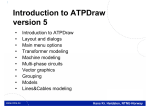
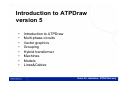
Introduction to ATPDraw
Multi-phase circuits
Vector graphics
Grouping
Hybrid transformer
Machines
Models
Lines&Cables
Hans Kr. Høidalen, NTNU-Norway
2
Introduction
• ATPDraw is a graphical, mouse-driven, dynamic
preprocessor to ATP on the Windows platform
• Handles node names and creates the ATP input file
based on ”what you see is what you get”
• Freeware
• Supports
–
–
–
–
–
All types of editing operations
~100 standard components
~40 TACS components
MODELS
$INCLUDE and User Specified Components
Hans Kr. Høidalen, NTNU-Norway
3
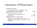
Introduction- ATPDraw history
• Simple DOS version
– Leuven EMTP Centre, fall meeting 1991, 1992
• Extended DOS versions, 1994-95
• Windows version 1.0, July 1997
– Line/Cable modelling program ATP_LCC
– User Manual
BPA
Sponsored
• Windows version 2.0, Sept. 1999
– MODELS, more components (UM, SatTrafo ++)
– Integrated line/cable support (Line Constants + Cable
Parameters)
Hans Kr. Høidalen, NTNU-Norway
4
Introduction- ATPDraw history
• Windows version 3, Dec. 2001
–
–
–
–
–
Grouping/Compress
Data Variables, $Parameter + PCVP
LCC Verify + Cable Constants
BCTRAN
User Manual @ version 3.5
• Windows version 4, July 2004
– Line Check
– Hybrid Transformer model
– Zigzag Saturable transformer
• Windows version 5, Sept. 2006
– Vector graphics, multi-phase cirucits, new file handling
Hans Kr. Høidalen, NTNU-Norway
5
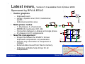
Latest news, Version 5.0 available from October 2006
Sponsored by BPA & EEUG
M
MODEL
fourier
•
Vector graphics
1
– Improved zoom
– Larger, dynamic icon; RLC, transformer,
switch…
– Individual selection area
•
Multi-phase nodes
–
–
–
–
•
LCC
132/11.3
I
Y
132 kV 22.2 mH
LCC
1..26 phases, A..Z extension
MODELS input/output X[1..26]
Connection between n-phase and single phase
21 phases in LCC components
1
LCC
SAT
LCC
POS
AC
New file management
– Project file follows the PKZIP 2 format.
Improved compression. acp-extension.
– Sup-file only used when a component is
created.
– External data moved from files to memory.
– Individual, editable help strings for all
components.
NEG
PULSE 1
4
3
6
5
2
6-phase
Hans Kr. Høidalen, NTNU-Norway
6
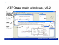
ATPDraw main windows, v5.2
Main menu
Tool bar
Component
bar (optional)
Header,
circuit file
name
Circuit
windows
Circuit
map
Component
selection menu
Circuit
under
construction
Hans Kr. Høidalen, NTNU-Norway
7
ATPDraw Component dialog
Hans Kr. Høidalen, NTNU-Norway
8
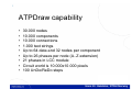
ATPDraw capability
•
•
•
•
•
•
•
•
•
30.000 nodes
10.000 components
10.000 connections
1.000 text strings
Up to 64 data and 32 nodes per component
Up to 26 phases per node (A..Z extension)
21 phases in LCC module
Circuit world is 10.000x10.000 pixels
100 UnDo/ReDo steps
Hans Kr. Høidalen, NTNU-Norway
9
ATPDraw Edit options
• Multiple documents
– several circuit windows
– large circuit windows (map+scroll)
– grid snapping
• Circuit editing
– Copy/Paste, Export/Import, Rotate/Flip,
– Undo/Redo (100), Zoom, Compress/Extract
– Windows Clipboard: Circuit drawings, icons, text, circuit data
• Text editor
– Viewing and editing of ATP, LIS, model files, and help files
• Help file system
– Help on ATPDraw functionality, all components, and MODELS
Hans Kr. Høidalen, NTNU-Norway
10
All standard components:
Hans Kr. Høidalen, NTNU-Norway
11
ATPDraw node naming
• "What you see is what you get"
• Connected nodes automatically get the
same name
– Direct node overlap
nodes connected nodes overlap
– Positioned on connection
• Warnings in case of duplicates and
disconnections
• 3-phase and n-phase nodes
Connection
– Extensions A..Z added automatically
1
– Objects for transposition and splitting
– Connection between n- and single
Transposition Splitter
phase
ABC
Hans Kr. Høidalen, NTNU-Norway
12
User’s manual
• Documents version 3.5 of ATPDraw (246 pages), pdf
• Written by Laszlo Prikler and H. K. Høidalen
• Content
–
–
–
–
Intro: To ATP and ATPDraw + Installation
Introductory manual: Mouse+Edit, MyFirstCircuit
Reference manual: All menus and components
Advanced manual: Grouping/LCC/Models/BCTRAN + create
new components
– Application manual: 9 real examples
Hans Kr. Høidalen, NTNU-Norway
13
Files in ATPDraw
• Project file (acp): Contains all circuit data.
• Support file (sup): Component definitions. Used only
when a component is added to the project.
– Standard components: ATPDraw.scl
– User defined components: Optionally in global library
• Data file (alc/bct/xfm): Contain special data
– Stored internally in data structure
– Optionally in global library
• Help file (sup/txt): User specified help text
– Global help stored in sup-file or /HLP directory (txt file)
– Local help created under Edit definitions
+
Hans Kr. Høidalen, NTNU-Norway
14
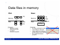
Data files in memory
Old:
New:
obj
Memory
Disk
Memory
data
sup
Problems:
• Where? Lots of
files/messy disk
• Conflicts
between projects
obj
Disk
data
import/export
Library
Solutions:
• No files extracted to disk
• Import/Export allowed
• Clear distinction between
global library and projects
• No conflicts between
projects
Hans Kr. Høidalen, NTNU-Norway
15
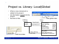
Project vs. Library: Local|Global
•
•
•
When a new component is
added to the project:
All information copied into the
project
No links to files
Edit global data
ATPDraw
Memory
Circuit
project
Edit local data
Library
Disk
New/Import
Export/Save as
Make ATP file
Run ATP
ATPDraw.scl
User specified
Models
Line&Cables
Bctran/XFMR
/USP
/MOD
/LCC
/BCT
/ResultDir:
User Specified and
Line&Cable include files
Hans Kr. Høidalen, NTNU-Norway
16
Result Directory
• The user initially specifies where the result should be
stored (ATP and $Include files)
• ATPDraw.ini in APPDATA/ATPDraw
Hans Kr. Høidalen, NTNU-Norway
17
Vector graphics
A
A
SAT
• Sponsored by EEUG (2007)
• Better zooming and dynamics
• Increased icon size 255x255 (from 41x41)
• Allow more nodes than 12
MODEL
large
• Additional: Flipping & Individual scalable icons
SM
SM
ω
ω
Hans Kr. Høidalen, NTNU-Norway
18
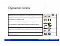
Dynamic icons
RLC, RLC3, RLCD3, RLCY3; R, L, C, RL, RC, LC, RLC appearance.
PROBE_I (Current probe); Single phase or three phase appearance.
I
LCC; Overhead line, single core cable, or enclosing pipe appearance. Length
of transmission line optionally added.
I
LCC
LCC
5.09 km
50. km
All sources; current (rhomb) or voltage (circle) source appearance.
Universal machines; manual/automatic initialization, neutral grounding.
SM
IM
ω
ω
TSWITCH (Time controlled switch); opening/closing indications.
Transformers; Coupling (Wye, delta, auto, zigzag), two/three windings.
XFMR
A
Y
A
SAT
TACS summation. Positive (red), negative (blue), or disconnected input. Click
on the nodes to activate.
RMS
G(s)
66
Hans Kr. Høidalen, NTNU-Norway
19
Vector icon editor
• Difficult for the user to change the default icons
– Vector elements
– Node positions
• Vector editor is text based.
Shapes:
– Shapes and Texts
Hans Kr. Høidalen, NTNU-Norway
20
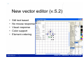
New vector editor (v.5.2)
•
•
•
•
•
Still text based
No mouse response
Visual response
Color support
Element ordering
Hans Kr. Høidalen, NTNU-Norway
21
Multi-phase circuits
• EEUG sponsored project
• Why?
– Problems and bugs related to the Splitter
– Better support of MODELS input/output arrays
– Need for multi-phase communication in Groups
and Models
Hans Kr. Høidalen, NTNU-Norway
22
Principles
• Nodes and connections extended to 26-phase (A..Z
node name extension)
• Only 3-phase nodes transposed
• Model arrays X[1..26] supported
• Special connection between single phase and nphase node
• Connection properties: Color, label, phase carried
• Extended Probe capabilities
• LCC module capability increased to 21 phases
Hans Kr. Høidalen, NTNU-Norway
23
Example 1
• Single phase to 3-phase connection
Old:
New:
LCC
LCC
1
LCC
LCC
• The Splitter carries Transpositions the single phase
connection not.
Hans Kr. Høidalen, NTNU-Norway
24
Example 2
•
Multi-phase connections
Freq
T
T
K
x
x
y
y
T
+
Freq
T
T
T
+
Gu
Angle
T
T
1
4
3
6
5
2
-
58
54
54
54
54
54
54
x
x
y
y
180
1
2
3
4
5
6
6-phase
•
Increased circuit readability
Hans Kr. Høidalen, NTNU-Norway
25
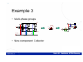
Example 3
• Multi-phase groups
POS
T
+
AC
AC
1
3
POS
+
-
LCC
NEG
T
-
PULSE
Y
Y
SAT
NEG
PULSE 1
4
3
6
5
2
6-phase
• New component: Collector
Hans Kr. Høidalen, NTNU-Norway
26
MODEL FOURIER
INPUT X
--input signal to be transformed
DATA FREQ {DFLT:50} --power frequency
n {DFLT:26}
--number of harmonics to calculate
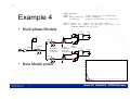
Example 4
OUTPUT absF[1..26], angF[1..26],F0 --DFT signals
VAR
absF[1..26], angF[1..26],F0,reF[1..26], imF[1..26],
i,NSAMPL,OMEGA,D,F1,F2,F3,F4
• Multi-phase Models
5 uH
5 mF
UI
MODEL
fourier
Cab le
Y
Y
Y
V
U(0)
+
M
0.0265
Z
SAT
SAT
1
HVBUS
132/11.3
I
Y
Y
Y
Y
Y
SAT
• New Model probe
Z
SAT
V
5 mF
U(0)
Cab le
5 uH
+
132 kV 22.2 mH
Regulation
transformers
11.3/10.6 kV
UI
SAT
Diode
Zig-zag
b ridges
transformers
ZN0d11y0
10.7/0.693 kV
0.0265
20
16
12
8
4
0
0.02
0.03
0.04
(f ile Exa_14.pl4; x-v ar t) m:X0027E
0.05
m:X0027G
0.06
m:X0027V
0.07
0.08
0.09
[s]
0.10
m:X0027Y
Hans Kr. Høidalen, NTNU-Norway
27
Example 5
• Extended Probe capabilities
– Monitor 1-26 phases
– Read and display steady-state values
-56.7+j22.18
I
Hans Kr. Høidalen, NTNU-Norway
28
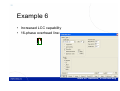
Example 6
• Increased LCC capability
• 16-phase overhead line:
LCC
Hans Kr. Høidalen, NTNU-Norway
29
Grouping
• Select a group (components, connections, text)
• Click on Edit|Compress
• Select external data/nodes
GROUP
mech
Hans Kr. Høidalen, NTNU-Norway
30
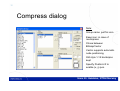
Compress dialog
Note:
Group name: just for icon
Keep icon: in case of
recompress
Chose between
Bitmap/Vector
Vector supports automatic
node positioning
Old style 1-12 borderpos
kept
Specify Position=0 to
enable (x, y) pos.
Hans Kr. Høidalen, NTNU-Norway
31
Grouping - special
• Data with the same name appear only once in the
input dialog
– Data value copied
– Double click on name to change
• Nonlinear characteristic supported
Hans Kr. Høidalen, NTNU-Norway
32
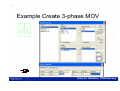
Example Create 3-phase MOV
Hans Kr. Høidalen, NTNU-Norway
33
Example – Induction motor
• Induction motor fed by a pulse width modulated
voltage source
• External mechanical load
V
BUS
PULS
SQPUL
FS
VDELTA
AMPL
SIGC
SIGA
VD
USMG
BUSMS
I
Torque
U
Hans Kr. Høidalen, NTNU-Norway
34
Examples
• 3-phase RMS-meter
in
out
• Lightning-induced voltage in 2-phase overhead line
left
right
U
U
U
U
Hans Kr. Høidalen, NTNU-Norway
35
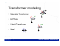
Transformer modeling
Y
Z
• Saturable Transformer
SAT
BCT
Y
• BCTRAN
• Hybrid Transformer
XFMR
Y
• Ideal
P
n: 1
S
Y Y
Hans Kr. Høidalen, NTNU-Norway
36
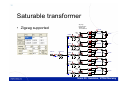
Saturable transformer
Zig-zag
transformers
ZN0d11y0
10.7/0.693 kV
• Zigzag supported
V
26.5mohm
5 uH
transformers
11.3/10.6Ydy
kV
Y
Y
SAT
Y
V
26.5mohm
Y
SAT
SAT
22.2 mH
V
Y
V
26.5mohm
Z
SAT
SAT
V
Y
SAT
V
26.5mohm
+
Y
Y
5 uH
UI
Zdy
+12
Cab le
+
Y
Y
5 uH
UI
Zdy
+6
Cab le
+
Cab le
Y
5 mF
SAT
UI
Y
5 mF
Z
V
132/11.3
U(0)
V
+
Y
Y
5 uH
UI
Zdy
-6
SAT
132 kV
5 mF
SAT
V
Y
5 mF
Z
SAT
Cab le
5 mF
U(0)
26.5mohm
U(0)
V
U(0)
Y
U(0)
Y
Y
+
Cab le
UI
Zdy
-12
5 uH
Z
SAT
Hans Kr. Høidalen, NTNU-Norway
37
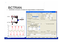
BCTRAN
• Automatic inclusion of external magnetization characteristic
XFMR
V
V
V
Y
XFMR
I
16 kV
BCT
V
V
Y
I
BCTRAN
80
[A]
50
20
-10
-40
-70
0.00
0.02
0.04
(f ile Exa_16.pl4; x-v ar t) c:X0004A-LV_XA
0.06
0.08
[s]
0.10
c:X0004A-LV_BA
Hans Kr. Høidalen, NTNU-Norway
38
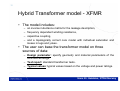
Hybrid Transformer model - XFMR
• The model includes:
–
–
–
–
an inverse inductance matrix for the leakage description,
frequency dependent winding resistance,
capacitive coupling,
and a topologically correct core model with individual saturation and
losses in legs and yokes.
• The user can base the transformer model on three
sources of data:
– Design parameter: specify geometry and material parameters of the
core and windings.
– Test report: standard transformer tests.
– Typical values: typical values based on the voltage and power ratings.
Hans Kr. Høidalen, NTNU-Norway
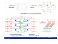
39
1. Physical
Structure
2. Magnetic
Circuit
3. Dual Electric Circuit, Hybrid Model
– Core representation
– Leakage representation
w– Resistance
w– Capacitive effects
Hans Kr. Høidalen, NTNU-Norway
40
– Leakage representation
•
•
•
•
Corresponds to the [A] = [L]-1 matrix
Takes into account the coils turn ratios
Introduces artificial N+1th winding at core surface
No mutual coupling between the phases
equivalent core is attached to
a fictitious N+1th winding
Hans Kr. Høidalen, NTNU-Norway
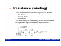
41
– Resistance (winding)
•
Their dependence on the frequency is due to
–
–
–
•
Skin effects
Proximity effects
Eddy currents
The frequency-dependency of R is represented
using Foster equivalent circuit (two cells)
Hans Kr. Høidalen, NTNU-Norway
42
– Capacitive effects
•
•
Capacitances between high and low voltage windings
and core
Capacitance between high voltage phases, outer legs,
and grounded elements
Hans Kr. Høidalen, NTNU-Norway
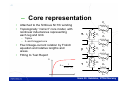
43
– Core representation
Out
Attached to the fictitious N+1th winding
Topologically “correct” core model, with
nonlinear inductances representing
each leg and limb
Ll
Leg
•
•
Ro
Rl
Lo
Ry
Rl
Ly
Ry
Rl
Ly
Ro
Yoke
Leg
Ll
Ll
i
λ=
a'+b'⋅ | i |
Out
•
Flux linkage-current relation by Frolich
equation and relative lengths and
areas.
Fitting to Test Report
λ
Leg
•
Yoke
– Triplex
– 3- and 5-legged core
i
Lo
Hans Kr. Høidalen, NTNU-Norway
44
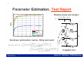
Parameter Estimation, Test Report
20
Relative areas and lengths
18
i5 =
16
14
l y ⋅ a ⋅ (λ1 − λ λ )
Ay − b ⋅ λ1 − λ λ
lambda
12
10
8
6
mid legs
outer legs
yokes
starting points
0
0
10
20
30
40
50
60
70
i
Nonlinear optimization routine, fitting test report
1
2
2
4
5-legged core
Hans Kr. Høidalen, NTNU-Norway
45
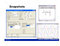
Snapshots
Hans Kr. Høidalen, NTNU-Norway
46
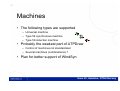
Machines
• The following types are supported
– Universal machine
– Type 59 synchronous machine
– Type 56 induction machine
IM
ω
SM
IM
T
• Probably the weakest part of ATPDraw
– Control of machines not standardized
– Several machines (combinations) ?
• Plan for better support of WIndSyn
Hans Kr. Høidalen, NTNU-Norway
47
Type 56 machine
• Initial support in ATPDraw
– Improvements required (TACS control, combination with UM)
• Brand new versions of ATP and PlotXY required
• More numerically stable (phase domain)
• Limitations on the mechanical side and in rotor coils
V
V
TACS
INIT
UM 1
IM
T
TACS
INIT
Type
56
IM
ω
M
T
T
Hans Kr. Høidalen, NTNU-Norway
48
Models
• ATPDraw reads the Model text and identifies the circuit
components with input/output/data
• Automatic creation of icon
– User who insists on a special icon should create global Models in
Library
• Indexed Nodes and Data supported
• Create a Model from scratch or load a predified Model
Hans Kr. Høidalen, NTNU-Norway
49
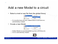
Add a new Model to a circuit
• Select a mod or sup file from the global library
– If a sup-file does not exist, default data is used and icon
automatically created
• Create a new Model
– Default Model is used (ModelDef.sup from ATPDraw.scl)
– Icon is automatically created
MODEL
default
Hans Kr. Høidalen, NTNU-Norway
50
Edit a Model in a circuit
• In the Component dialog box click on Edit
Right click
• The built-in text editor appears
– Edit the text/Import
– Click on Done
• Respond to the Model identified message
Hans Kr. Høidalen, NTNU-Norway
51
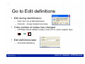
Go to Edit definitions
• Edit during identification
– Click Yes: Go to Edit definitions
– Click No: Accept default icon/node
• If the number of nodes has changed
– ATPDraw will as default create a new icon in vector graphic style
MODEL
flash_1
• Edit definitions later
– Click Edit definitions
Hans Kr. Høidalen, NTNU-Norway
52
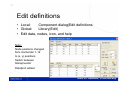
Edit definitions
• Local:
Component dialog|Edit definitions
• Global:
Library|Edit|
• Edit data, nodes, icon, and help
Note:
Node positions changed
from iconborder 1-12
to (x, y) positions
Switch between
bitmap/vector
Data|Unit added
Hans Kr. Høidalen, NTNU-Norway
53
Example – Transformer tester
• Pocket calculator
• RMS and Power calculation
• TTester: Averaging, printout
M
M M M
M
M
ResultDir\model.1
I
V XFMR
V
Y
87.5003664
93.7503926
100.000419
106.250445
112.500471
.17121764 131.434758
.220581306 151.751037
.35109472 173.603833
.743208151 196.896531
2.85953651 221.288092
Hans Kr. Høidalen, NTNU-Norway
54
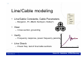
Line/Cable modeling
• Line/Cable Constants, Cable Parameters
– Bergeron, PI, JMarti, Semlyen, Noda(?)
• View
– Cross section, grounding
log(| Z |)
3.9
• Verify
– Frequency response, power frequency params.
2.7
1.5
• Line Check
– Power freq. test of line/cable sections
log(freq)
0.4
0.0
2.0
4.0
6.0
Hans Kr. Høidalen, NTNU-Norway
55
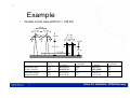
Example
•
Double circuit case (420 kV + 145 kV)
12 m
11 m
11 m
4.5 m
9.6 m
4.5 m4.5 m
3.8 m
18.6 m
35.5 m
Test type
Benchmark data
50 Hz, 100 Ωm
Individual testing
Bergeron model
Circuit
[kV]
420
145
420
145
11 m
Positive sequence system
C [nF/km]
Z [Ω/km]
0.02+j0.29
12.8
0.06+j0.38
9.7
0.02+j0.29
12.8
0.06+j0.38
9.7
Zero sequence system
C [nF/km]
Z [Ω/km]
0.19+j0.71
9.3
0.25+j0.80
6.7
0.18+j0.71
9.3
0.25+j0.80
6.9
Hans Kr. Høidalen, NTNU-Norway
56
Creating the Bergeron model
Hans Kr. Høidalen, NTNU-Norway
57
Testing the Bergeron model
•
Line Model Frequency scan. Model OK for 50 Hz.
Hans Kr. Høidalen, NTNU-Norway
58
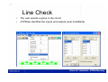
Line Check
•
•
The user selects a group in the circuit
ATPDraw identifies the inputs and outputs (user modifiable)
Hans Kr. Høidalen, NTNU-Norway
59
Line Check cont.
•
ATPDraw reads the lis-file and calculates the series impedance
and shunt admittance
Hans Kr. Høidalen, NTNU-Norway
60
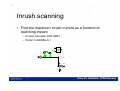
Inrush scanning
• Find the maximum inrush current as a function of
switching instant
– Pocket calculator KNT+MNT
– Write1 to MODELS.1
MODEL
max
I
2
I
2
BCT
Y
XFMR
Y
Hans Kr. Høidalen, NTNU-Norway