1
CURAÇAO
Version 2.2
User’s Manual
Phil A. Arneson
Barr E. Ticknor
Cornell University
Cornell University
A BioQUEST Library VII Online module published by the BioQUEST Curriculum Consortium
The BioQUEST Curriculum Consortium (1986) actively supports educators interested in the
reform of undergraduate biology and engages in the collaborative development of curricula.
We encourage the use of simulations, databases, and tools to construct learning environments
where students are able to engage in activities like those of practicing scientists.
Email: [email protected]
Website: http://bioquest.org
Editorial Staff
Editor:
Managing Editor:
Associate Editors:
John R. Jungck
Ethel D. Stanley
Sam Donovan
Stephen Everse
Marion Fass
Margaret Waterman
Ethel D. Stanley
Online Editor:
Amanda Everse
Editorial Assistant: Sue Risseeuw
Beloit College
Beloit College, BioQUEST Curriculum Consortium
University of Pittsburgh
University of Vermont
Beloit College
Southeast Missouri State University
Beloit College, BioQUEST Curriculum Consortium
Beloit College, BioQUEST Curriculum Consortium
Beloit College, BioQUEST Curriculum Consortium
Editorial Board
Ken Brown University of Technology, Sydney, AU
Joyce Cadwallader St Mary of the Woods College
Eloise Carter Oxford College
Angelo Collins Knowles Science Teaching Foundation
Terry L. Derting Murray State University
Roscoe Giles Boston University
Louis Gross University of Tennessee-Knoxville
Yaffa Grossman Beloit College
Raquel Holmes Boston University
Stacey Kiser Lane Community College
Peter Lockhart Massey University, NZ
Ed Louis The University of Nottingham, UK
Claudia Neuhauser University of Minnesota
Patti Soderberg Conserve School
Daniel Udovic University of Oregon
Rama Viswanathan Beloit College
Linda Weinland Edison College
Anton Weisstein Truman University
Richard Wilson (Emeritus) Rockhurst College
William Wimsatt University of Chicago
Copyright © 1993 -2006 by Phil A. Arneson and Barr E. Ticknor
All rights reserved.
Copyright, Trademark, and License Acknowledgments
Portions of the BioQUEST Library are copyrighted by Annenberg/CPB, Apple Computer Inc., Beloit College, Claris
Corporation, Microsoft Corporation, and the authors of individually titled modules. All rights reserved. System 6,
System 7, System 8, Mac OS 8, Finder, and SimpleText are trademarks of Apple Computer, Incorporated. HyperCard
and HyperTalk, MultiFinder, QuickTime, Apple, Mac, Macintosh, Power Macintosh, LaserWriter, ImageWriter, and the
Apple logo are registered trademarks of Apple Computer, Incorporated. Claris and HyperCard Player 2.1 are
registered trademarks of Claris Corporation. Extend is a trademark of Imagine That, Incorporated. Adobe, Acrobat, and
PageMaker are trademarks of Adobe Systems Incorporated. Microsoft, Windows, MS-DOS, and Windows NT are
either registered trademarks or trademarks of Microsoft Corporation. Helvetica, Times, and Palatino are registered
trademarks of Linotype-Hell. The BioQUEST Library and BioQUEST Curriculum Consortium are trademarks of Beloit
College. Each BioQUEST module is a trademark of its respective institutions/authors. All other company and product
names are trademarks or registered trademarks of their respective owners. Portions of some modules' software were
created using Extender GrafPak™ by Invention Software Corporation. Some modules' software use the BioQUEST
Toolkit licensed from Project BioQUEST.
TABLE OF CONTENTS
ABOUT THIS MANUAL................................................................................................................2
INSTALLATION AND QUICK INSTRUCTIONS .......................................................................2
THE STERILE INSECT RELEASE METHOD...........................................................................3
MODEL DESCRIPTION ...............................................................................................................5
The Basic Model ...........................................................................................................................5
Assumptions of the Default Model ................................................................................................5
Variations on the Model................................................................................................................6
Spatial resolution .......................................................................................................................... 6
Order of events ............................................................................................................................. 6
Density Dependence ...................................................................................................................... 6
Stochastic simulation ..................................................................................................................... 7
Competitiveness ........................................................................................................................... 7
Spatial heterogeneity ..................................................................................................................... 8
Estimation of native population size.................................................................................................. 8
Number of sterile insects released..................................................................................................... 8
PROGRAM FEATURES................................................................................................................9
File Menu......................................................................................................................................9
Insects Menu............................................................................................................................... 10
View Menu.................................................................................................................................. 11
Show/Hide Grid.......................................................................................................................... 11
Population Levels........................................................................................................................ 12
Summary Window ...................................................................................................................... 12
TUTORIAL and SUGGESTED EXERCISES.............................................................................13
REFERENCES .............................................................................................................................18
Page i
LEGAL DETAILS
Curaçao is based on the work of A. J. Sawyer et al. (1987). The simulation has been refined
and adapted to the Microsoft« WindowsTM environment (ver. 3.0 or higher) by Phil Arneson and
Barr Ticknor, Department of Plant Pathology, Cornell University.
The following files should be kept together in the same folder:
CURACAO.EXE - the main program
KEYHOOK.DLL - the keyhook library which supports the context sensitive help
system.
CURACAO.HLP - the help file
CURACAO.WRI - the manual in Microsoft Windows Write format
Page 1
ABOUT THIS MANUAL
Throughout the manual, menu names are printed in Italics. Menu commands and the names
of buttons and other controls are given in Boldface. Individual keys are indicated by the name of
the key enclosed in angle brackets; thus, <Enter> represents the Enter key. Two or more keys
joined by a "+" represent a key combination. For example, <Alt>+<Tab> indicates that you
should press and hold the Alt key while pressing the Tab key.
INSTALLATION AND QUICK INSTRUCTIONS
Curaçao will run on any system which supports Microsoft Windows. A mouse is required, and
a math coprocessor is strongly recommended.
To install, insert the BioQUEST Library CD that is compatible with the Windows operating
system into the appropriate drive of your computer. Open the Online Guide. Using the
instructions on the first page of the Online Guide, navigate to the "Curaçao" section of the Guide.
Clicking on the Install button on the bottom of the page will start the installation process. Follow
the instructions on the screen.
Note: To use the Online Guide, the Acrobat Reader must be installed on your computer. For best
results, we suggest that you install Acrobat Reader version 4.0 or later. An installer for Reader
version 4.0 is included on the BioQUEST Library CD.
Run CURACAO.EXE just as you would any other Microsoft Windows program. If you don't
change any of the program options, it will simulate the model conceived by E. F. Knipling,
whose early work with this method of pest control led to the eradication of the screwworm from
the island of Curaçao. This is a good place to start. Select File Run to get things going, then use
the Generation button to advance the simulation one generation at a time. Curaçao features a
context sensitive help system which is accessed by pressing the <F1> key or using the Help
menu. Use the help system and this manual to learn more about the program as you go along.
By resizing and rearranging the windows, you can keep the manual and/or help system available
while you're using Curaçao.
Page 2
THE STERILE INSECT RELEASE METHOD
The sterile insect release method (SIRM) of pest population suppression was first conceived by
E. F. Knipling (1955). It sometimes goes by the names "sterile male technique" and "autocidal
control". The method consists of releasing large numbers of sterilized insects into the
environment to reduce the probability that members of a natural population of the same species
will successfully reproduce. The method has been associated almost exclusively with efforts to
eradicate particular species from well-defined and limited geographic areas. Simple
mathematical models devised by Knipling (1979) demonstrate that, in theory, the method can
bring about the total eradication of a defined population in a small number of generations. Its
practical feasibility has been demonstrated by the eradication of the screwworm, Cochliomyia
hominivorax, from the Caribbean island of Curaçao and peninsular Florida, and the elimination
of isolated infestations of the Mediterranean fruit fly, Ceratitis capitata, other fruit flies, and the
gypsy moth, Lymantria dispar. It has also been applied in trial programs against the cotton boll
weevil, Anthonomus grandis, mosquitoes and the codling moth, Cydia pomonella.
The method works as follows. Large numbers of insects are produced in a rearing facility
and are sterilized by radiation or chemical means. The sterilized insects are released into the
natural population in numbers sufficient to ensure that most wild individuals will mate with a
sterile insect, resulting in failure to produce viable offspring. Additional releases of the same
number of sterile insects are made in subsequent generations, so that the ratio of sterile to fertile
insects increases dramatically over time. Within a few generations, no fertile matings are likely
to occur and the wild population is eliminated. The method is fairly unique among insect control
tactics in that it operates in an inverse density-dependent, or destabilizing, way. As the size of
the target population becomes smaller and smaller, the effectiveness of a given number of
released, sterile insects increases. This feature is what makes eradication theoretically possible.
The method works best in conjunction with other approaches that first reduce the size of the
target population so that fewer sterile insects need be reared and released.
Success of the method depends on a number of assumptions that must hold true. Some of the
more important are:
1. Insects can be reared and sterilized in large quantities.
2. Methods exist for distributing the sterile insects throughout the target area so they thoroughly
mix with the wild population.
3. The release is timed to coincide with the reproductive period of the target insect.
4. The released, sterile insects compete successfully for mates in the natural environment.
5. The release ratio (sterile insects to native, fertile insects) is large enough to overcome the
natural rate of increase of the population, so that the trend in population size is
downward after the first release.
Page 3
6. The target population is closed; i.e., there is no immigration of fertile insects from outside the
release zone.
Calculating the required release ratio for a particular situation is difficult. This requires an
accurate estimate of the size of the natural population and its spatial distribution. It also requires
knowledge of the natural rate of increase of the population. For a number of reasons it may be
desirable to release only sterile males. This requires a way of separating the sexes in the rearing
facility, and knowledge of the sex ratio of the wild population.
Curaçao is a computer program that simulates the sterile insect release method and allows
the user to investigate the effects of several variables on the effectiveness of the method and
what happens when some of the basic assumptions of the model are relaxed or violated in some
way. The user should gain some understanding of the sorts of things that complicate the
application of the technique in situations that are more realistic than those assumed by Knipling
in his simple analyses.
Page 4
MODEL DESCRIPTION
Curaçao is a version of the original model by A. J. Sawyer et al. (1987), which has been
adapted to run under Microsoft Windows. It was written to illustrate the effects of changes in the
assumptions of the simple mathematical models of Knipling (1979). We have given it the name
"Curaçao" after the Caribbean island on which Knipling first demonstrated the feasibility of
sterile insect release by eradicating the screwworm fly.
The Basic Model
Curaçao is a discrete-time model with a time step of one generation of the target insect
population. The dynamics are represented by the following equation:
Nt+1 = Nt _ Pf _ Pm _ Pfm _ Fec _ S + I - E
where Nt and Nt+1 are the number of native adults in a given area (defined in the model by a
square cell) in generations t and t+1. Pf is the proportion of the population that is female, Pm is
the proportion of females that mate, Pfm is the proportion of mating females that mate with a
fertile male, Fec is the mean fecundity of a fertile female, S is the survival rate from egg to adult,
I is the number of adults immigrating into a particular cell, and E is the number emigrating. The
proportion of females that mate with fertile males is given by:
Pfm = M / (M + C _ SM)
where M is the number of native, fertile males, SM is the number of sterile males, and C is the
relative competivieness of the sterile males. The model assumes that only sterile males are
released and that females mate only once, at most.
Numbers are rounded to the nearest integer after each computation involving a separate life
stage or population process. Fractional individuals are never allowed to exist.
Assumptions of the Default Model
The default model uses the original assumptions of Knipling (1979). It is assumed that the
target population exists in a well-defined zone. Its initial size is 1,000,000 individuals, half male
and half female. The population will increase 5X each generation (up to a point) (200
eggs/female x 0.05 survival rate to the adult stage x 0.5 female = 5). There is no dispersal.
Sterile males are released in a ratio of 9:1 (sterile to fertile males). The population is distributed
uniformly throughout the zone, and the released insects are well mixed with the indigenous
population. Sterile males are completely competitive with wild males in mating with females.
The model is deterministic, in that the mean sex ratio, survival of immatures, proportion of
females mating with fertile males, and fecundity all apply exactly, even in extremely small
populations (those near extinction). Thus, random (stochastic) events do not occur and cannot
affect the outcome of a release program.
Page 5
Variations on the Model
Countless variations on the basic simuation can be made by changing parameter values or
even the structure and underlying assumptions of the model.
Spatial resolution
Three different levels of spatial resolution are possible: low, medium and high. With low
spatial resolution, a single, central cell constitutes one zone, and the six surrounding cells make
up a second zone. With medium spatial resolution, there are three zones with 7, 12, and 18 cells,
respectively. The high spatial resolution also has three zones, but with 19, 42, and 66 cells.
When a zone consists of more than one cell, the population may or may not be heterogeneous in
that zone (all cells need not have the same population density). With space there is the
possibility of movement, and you can specify emigration probabilities. This is the fraction of the
population that will leave each cell during the dispersal phase of each generation. For example, if
you specify an emigration rate of 0.01, one insect in a hundred will leave the cell in which it
developed and enter a neighboring cell during the dispersal period. Individuals leaving a cell
have an equal probability of moving to each of the six neighboring cells. If a cell is on the
boundary of the outermost zone, dispersing individuals leave the modelled area and disappear
into the sea. (They can't return.)
Order of events
The order in which events occur assumes that you timed your release of sterile insects to
occur just before the mating and dispersal of the native population. The order of events,
therefore is: Release (of sterile males), Mating, Dispersal (if any). Two other orderings are
possible: release, dispersal, mating and dispersal, release, mating. This can be changed to
represent different life histories or release strategies.
Density Dependence
Four factors in the model can be made density-dependent. Normally it is assumed that all
females mate. In the density-dependent mode, however, the probability of mating is given by:
PMating = 1 - (1 - p1)N
where p1 is the probability of an individual female being discovered by a particular male in the
same cell, and N is the number of males in the cell. The parameter p1 is set to 0.01. At N = 500,
PMating is nearly 1.0.
In the density-dependent mode, fecundity and survival are both reduced by a factor (f) as egg
density reaches high levels:
f = (1 - Eggs / Maxeggs)0.5
Page 6
where Maxeggs is set to a value of 109 per cell. In the case of density-dependent fecundity, Eggs
is the density in the previous generation and represents the population density to which maturing
females were subjected at their site of origin. For density-dependent survival, Eggs is the density
at the site of oviposition. Fecundity is allowed to decline to a level just sufficient for
maintenance of the population, while survival is limited to a minimum value of 0.01.
In the density-dependent model, the probability of emigration from a cell increases from its
specified value, Pe (unless Pe = 0), to a maximum value as adult density reaches a high value:
DDE = PeMax + (Pe - Pe Max) _ (1 - Adults / MaxAdults)0.5
where DDE is the density dependent emigration rate, Adults is the number of adults, Maxadults
is 109 per cell, and Pe Max is 0.5. When Pe has been set to 0.0 by the user, it is assumed that
dispersal does not take place under any circumstances. (See Sawyer et al. (1987) for graphs of
these functions.)
Stochastic simulation
The model can be changed to a stochastic one in which random events play a role, especially
in small populations. Because the SIRM is concerned with what happens to a very small
population, this is an important feature. For example, when the remaining population is less than
100 or so, the mean sex ratio, survival of immatures, outcome of mating and fecundity may
depart from expected values just by chance. That last female may just happen to mate with a
fertile male even though it is unlikely. A fertile female might disperse to a neighboring cell
outside of the release zone, and initiate a new infestation, even though the chances of this
happening are small. The stochastic option generates random variates in the processes that
determine the numbers of:
- Wild female adults
- Females that mate
- Matings that are with fertile males
- Adults that emigrate from a cell
- Eggs carried by fertile females
- Offspring that survive to adulthood
The destinations of emigrating adults are also determined randomly with the stochastic
option. The stochastic version takes much more computation time because random events must
be generated for each individual, with probabilities drawn from appropriate distibutions having
the expected values as in the deterministic version.
Competitiveness
The competitiveness of released sterile males can be set to some value less than 1.0. This
parameter represents the relative value of the released males in competing for mates on an equal
basis with native males. For example, a release of 100,000 sterile males whose mean
competiveness is 0.8 is equivalent to a release of 80,000 fully competitive sterile males. In
Page 7
competition with 100,000 indigenous males, 40% of the mating will be with sterile males
(80,000/200,000). As in Knipling's basic model, we assume that all females mate (except at very
low densities, when some may fail to find mates), and females mate only once. Incidently, this
last assumption is not a necessary one for the application of theSIRM. With other mating
systems, the mathematics used to calculate the expected outcome of a release are different, but
the technique still works. Its efficiency depends on the reproductive details of each species.
Spatial heterogeneity
The initial population can be made homogeneous within a zone, or can vary from cell to cell
(with the correct overall mean). To achieve heterogeneity, an aggregation index can be specified
for each zone. This parameter is actually the coefficient of variation (S. D./mean) for individual
cell densities. (A value of 0.30 is somewhat clumped, while 1.00 is very clumped). Use 0.0 for
a uniformly distributed population. The cell densities are drawn from a gamma distribution with
the appropriate mean and variance.
Estimation of native population size
The release of sterile males can be based on the actual size of the target population, or on an
estimate of that population size. The latter is more realistic, since in practice a sampling survey
must be conducted to determine the population size prior to a release. Of course, sampling is
subject to error. In this model, the standard error of an estimate of population density is assumed
to be 40% of the mean, and an estimate is drawn from the appropriate normal distribution.
Sterile insects may be released on a zone basis or on a cell-by-cell basis. That is, the desired
release ratio may apply to the (actual or estimated) population of an entire zone, in which case
the same number of insects is released in each cell of the zone, or the ratio may apply to the
(actual or estimated) population in each individual cell. In this case different numbers of sterile
insects may be released in each cell. In a real field program, this would require greater sampling
effort and a more highly refined distribution system but would assure more efficient matching of
the actual release ratio to that which is intended (particulary for a patchily-distributed target
popuation).
Number of sterile insects released
Finally, you may specify a total number of sterile insects to release in each zone, without
regard to the ratio of sterile to fertile males. This is useful if a buffer zone, in which sterile
insects are released outside of the area of infestation, is needed.
Page 8
PROGRAM FEATURES
File Menu
Run
begins execution of the simulation.
Options...
allows you to make changes in the structure of the model. The options are:
Spatial Resolution
With low spatial resolution, a single, central cell constitutes one zone, and the six surrounding
cells make up a second zone. With medium spatial resolution, there are three zones with 7, 12,
and 18 cells, respectively. The high spatial resolution also has three zones, but with 19, 42, and
66 cells.
Order of Events
You can select one of three possible orders of events to represent the behaviors of different
insects and the timing of your release relative to those events:
Release->Mate->Disperse
Release->Disperse->Mate
Disperse->Release->Mate
Deterministic vs. Stochastic Simulation
This determines whether or not random chance has an effect on the outcome of the simulation, as
described above under Stochastic Simulation.
Density Dependence/Independence
This option determines whether the current population density will have an effect on certain
population processes (see above).
Log to disk...
allows you to open a text file that will keep a running log of your simulations. If this option is
chosen after a number of generations have been executed, all generations starting with the first
will be included in the log.
New
resets the native and released insect populations to their original values, allowing you to run the
model again.
Open...
allows you to open a file in which you have stored the options, parameters, and initial values for
a particular simulation or the state of the system at the moment in which you executed the Save
as... command in a previous run.
Page 9
Save as...
allows you to save in a disk file the complete state of the simulation (options, parameters,
graphics, and text) at the moment the command is executed. If you save a file called
STARTUP.SIR, it will be loaded automatically when Curaçao starts up. In this way, it is
possible to override the built-in defaults of the program.
Exit
exits Curaçao.
Insects Menu
Native...
allows you to set the initial populations of native insects in each of 3 zones and to set the native
population parameters, including the aggregation index, the probability of emigration, the
proportion female, the eggs/female, and the survival to adult.
Total Population
The island is divided into three concentric zones (only two zones with the low spatial resolution
option), and you can set the initial population of native insects in each zone by entering the
desired number in the appropriate box.
Aggregation Index
Knipling's original model assumed uniform distribution of the native insects. In Curaçao you
can create spatial variability and adjust the degree of aggregation by assigning a nonzero value to
the aggregation index. This parameter is actually the coefficient of variation (standard
deviation/mean). A value of 0.0 gives a uniform distribution, while a value of 1.0 gives a
severely clumped distribution.
Probability of Emigration
This parameter sets the proportion of the population in each cell that will leave that cell during
the dispersal phase of each generation. Individuals leaving a cell have an equal probability of
moving to each of the six neighboring cells. If a cell is on the boundary of the outermost zone,
dispersing individuals leave the modelled area and disappear into the sea!
Proportion Female
This parameter sets the proportion of the native insect population that is female.
Eggs per Female
This parameter sets the number of eggs produced per female. This parameter along with the
Survival to Adult and Proportion Female determines the normal trend of the population.
Survival to Adult
This parameter sets the proportion of eggs that survive to the adult stage. This parameter along
with Eggs per Female determines the normal trend of the population.
Page 10
Release by Zone...
allows you to set the initial release ratios (sterile:fertile) or initial release numbers in each zone.
You can also set the relative competitiveness of the released males. The release of sterile males
in each zone can be by numbers of males or by the ratio of sterile male to fertile males. The
sterile:fertile ratio can be determined by exact knowledge of the native population or by an
estimate of the native population that varies randomly according to a normal distribution with a
standard error equal to 40% of the mean population.The relative competitiveness of the released,
sterile males to the native, fertile males for mating success can be set to 1.0 (sterile and fertile
males equally competitive) or a value less than 1.0.
Release by Cell...
allows you to set the initial release ratios (sterile:fertile) or initial release numbers cell by cell.
You can also set the relative competitiveness of the released males. The release of sterile males
in each cell can be by numbers of males or by the ratio of sterile male to fertile males. The
sterile:fertile
ratio can be determined by exact knowledge of the native population or by an estimate of the
native population that varies randomly according to a normal distribution with a standard error
equal to 40% of the mean population.
Sterile males can be released in all cells (in which case the release ratios are determined cellby-cell, according to the initial populations of native males in each cell), or specific cells can be
marked for release of sterile males. If the marked cells only option is turned on, the cells can be
marked only after clicking OK in this dialog box, initiating execution by selecting File, Run,
and then selecting Insects, Mark Cells. Cells are marked by double clicking when the cursor is
on the desired cell. Marked cells (those that contain circles) can be unmarked by double clicking
on them. When all the desired cells have been marked, select Quit Marking from the Insects
menu.
The relative competitiveness of the released, sterile males to the native, fertile males for
mating success can be set to 1.0 (sterile and fertile males equally competitive) or a value less
than 1.0.
Mark Cells
allows you to mark the cells in which you would like to release sterile insects. This command is
available only if you have selected Release by Cell... and Release in marked cells only. The
cell marking function becomes operative only after the "map" has been created by selecting File,
Run. Selecting the Insects menu then displays the command Mark Cells.
View Menu
Show/Hide Grid
In this model, the island of Curaçao is divided into a grid of square cells. All of the simulation
calculations are performed for each individual cell in each generation. The Show/Hide Grid
command in the View Menu allows you to choose whether or not the lines separating cells are
Page 11
drawn on the screen. For ease of reference, the cells are assigned coordinates as (row, column)
pairs. Holding down the mouse button while the arrow cursor is over a cell will cause that cell's
coordinates to be displayed.
Population Levels
The density of the native insect population is represented on a geometric scale of 1 to 10. Solid
green represents the lowest population density; solid yellow the highest. Intermediate levels are
represented by intermediate shades. The size of the population which will be represented as
level 10 can be set in the Population Levels dialog box, as can the factor relating each level to the
next.
For example, by default, level 10 represents a population of 10,000,000 insects per cell and the
factor is 10. Hence level 9 represents 1,000,000, level 8 is 100,000, and so on.
Summary Window
As you proceed with the simulation generation by generation, the Summary Window shows the
native insect population in each zone and the number of sterile males which have been released.
The Show/Hide Summary command in the View Menu allows you to control the presence of this
window. The Summary window can also be hidden by double clicking the close box in the
upper left corner of the window. The summary can be presented as columns of numbers (Text
Summary), or as a line graph which rescales automatically to fit the size of the window (Graphic
Summary).
Page 12
TUTORIAL and SUGGESTED EXERCISES
[These exercises are also available in a separate document called "Tutorial.doc".]
This tutorial assumes that you are already acquainted with Microsoft Windows. Therefore,
our instructions will focus on the model and the features unique to Curaçao. If you need help
with the Windows environment itself, go to the Help menu of either the Program Manager or
the File Manager. The information presented there explains the standard features of the
environment. These exercises begin with the simple Knipling (1979) model and then add
various levels of complexity to that original model. In each case, the results of the simulation
ought to be compared to those of the original Knipling model.
Saving a Startup File
As soon as you have started Curaçao, select Save As from the File menu. When the dialog
box appears prompting you for a file name, enter STARTUP.SIR. This will create a disk file
containing the default parameters for the simulation and and provide a convenient method of
restoring the defaults later. When Curaçao is started, it will look for a file with this name and
load it automatically if found. You can also open the file from the File menu. By changing
program parameters before saving STARTUP.SIR, you can override the defaults which are
written into the program.
Knipling's example
Recreate Knipling's example by executing the model without changing any of the parameters.
Select Run from the File menu. A picture of the island of Curaçao will appear with a shaded
square in the center representing the population of screwworm flies. Click on the Generation
button in the lower right corner of the window to advance the simulation one generation at a
time. Observe the numerical summary in the window on the right. In how many generations is
eradication achieved? How many sterile insects had to be released in total?
Minimum initial release ratio
Under the assumptions that Knipling used, eradication could have been achieved with a
lower ratio of released, sterile insects to native, fertile insects. Select New from the File menu.
Dismiss the dialog boxes that appear by clicking on No. Select Release by Zone from the
Insects menu. Change the initial release ratio in Zone 1 to 8.0. When you are satisfied with all
of the numbers in the window, click OK. Select Run from the File menu again, and step
through the generations as before. At the end of each run, you must select File, New. Decrease
the initial release ratio until you find the smallest initial release ratio (to the nearest tenth) that
will result in eradication. What is the minimum effective initial ratio of sterile to fertile males
that results in eradication, and how does this ratio relate to the normal trend? In how many
generations is eradication achieved at this ratio, and how many sterile insects must be released?
How does this compare with the results of the original Knipling example?
Page 13
Sterile male competitiveness
Select Open from theFile menu and reopen STARTUP.SIR to reset the default parameters.
In the Insects menu, again select Release by Zone, and change the competitiveness from 1.0 to
0.5. How many generations and how many total sterile insects are required for extinction at an
initial release ratio of 9.0 to 1? Now what is the minimum effective initial release ratio (to the
nearest tenth), and how many total insects must be released to achieve extinction? How does this
compare with the results of the original Knipling model?
Fecundity of females
Return to the default setup by reopening STARTUP.SIR, as before. Select Insects, Native.
Increase the fecundity of females from 200 to 300. Now how many generations and how many
sterile insects are required for extinction? What is the minimum effective initial release ratio in
this situation? How does this compare with the results of the original Knipling model?
Survival to adult
Return to the default setup again. Bring up the Insects, Native dialog box and increase the
rate of survival to adult from 0.05 to 0.08. How many generations and how many sterile insects
are required for extinction, and what is the minimum effective initial release ratio? How does
this compare with the results of the original Knipling model?
Initial release ratio based on population estimate
Base a release on an estimate of the native insect population in zone 1, rather than its exact
size (which you wouldn't know). To do this, return to the default setup again, and bring up the
Insects, Release by Zone dialog box. Click on the button that says ratios (estimated pop.).
This time your estimates of the native population (and therefore your actual release ratios) will
be different each time you run the model, varying about the mean according to a normal
distribution. And this time after selecting File, New and getting the dialog box, "Repeat the
same problem?", click on Yes. Run the model 10 times using the original initial release ratio of
9.0 and another 10 times using the minimum initial release that you determined in Step 2. (Note
that the text summary reports the actual total insect population and the actual numbers of
released sterile males.) How many times out of ten were you successful in eradicating the
population in each case? Why do you suppose Knipling used 9:1 as the initial release ratio in his
example?
Spatial aggregation
Return to the default setup, and select File, Options. Click on the first control until High
Resolution appears, then click OK. Next select Insects, Native, and set the Aggregation Index
(coefficient of variation) to 0.4. (Note that we are back to a ratio based on an exact estimate of
the initial population, but this time the spatial aggregation of the insects will be different for each
run. Note also that because of the additional computation required, the execution is slower than
with the low spatial resolution model.) Repeat this problem 10 times with an initial release ratio
Page 14
of 9.0. How many times were you successful in eradicating the native population? (Explain the
reason for any failures.) Set the Aggregation Index to 0.5 and repeat this problem 5 times. What
effect does the tighter aggregation have on the success of the sterile insect release method?
(Remember you are releasing the same initial population in Zone 1 in each case.)
Emigration
Now add the element of pest mobility to the spatial aspects just considered. Return to the
default setup. Select Insects, Native, and set the Aggregation Index to 0.4 and the Probability of
Emigration to 0.01 (1 insect in a 100 will leave each cell for one of the adjacent ones in each
generation). Run the same problem 5 times, and note the movement of the population each time.
(Once the population trend turns upward in Zone 2, there is no point in continuing with further
generations.) Check the populations of a few selected cells in Zone 2 in each generation by
moving the cursor to the desired cell and double clicking. A dialog box will tell you the
populations of native and sterile insects in that cell. Why is extinction of the population not
possible?
Border zone
To see the importance of establishing a border zone in attempting to eradicate a mobile pest,
return to the same problem as in the previous step by selecting File, New, and No. Keep the
same native insect population parameters as before (Total Population, Zone 1: 1000000;
Aggregation Index: 0.4; and Probability of Emigration: 0.01), but for the "Release by Zone"
change the Release by: from ratio (exact population) to numbers. Now release 4500000 sterile
males in Zone 1 (which gives the same 9:1 ratio), but this time also add 4500000 sterile males to
Zone 2. Repeat this same problem 10 times. Did you have any unsuccessful eradication
attempts? If so, what was the spatial nature of the population development?
Hot spots
Generally it is not enough simply to adjust release ratios based upon the initial assessment of
the native population, particularly where the populations are highly aggregated. It is necessary to
monitor the populations each generation and to increase the numbers of sterile insects released in
those areas where the population trend is not downward. Return to the same problem as in the
previous step by selecting File, New, and No, and increase the aggregation to 0.5 to increase the
chance of developing a "hot spot" (i.e., an area of high population density). Run the simulation,
and at each generation look for the development of cells where the population does not appear to
decline with successive generations. Double click on these cells as before to see the populations
of native and sterile insects. If the population of native males gives you a release ratio in the
current generation of less than about 5:1, release more sterile males in that cell by typing in a
value that corresponds to a release ratio of about 10:1 and clicking OK. Repeat this same
problem 5 times without any release ratio adjustments and 5 times with increases in release ratios
in the hot spots. How did the outcomes of these two approaches compare?
Page 15
Nonuniform release patterns
With the exception of the "hot spot" releases just completed, the simulations we have done so
far have assumed uniform distribution of the released sterile males, as they might be dispersed by
a release from an aircraft. Let us now look at what might happen with a cell-by-cell release, as if
we had to place caged insects in specific sites. To avoid having to mark too many cells, first
reduce the spatial resolution by selecting File, Options... and selecting Medium Spatial
Resolution. To increase our chances of success, we will do this with an insect that has a
dispersal phase before mating, and we will time our release to occur just before this dispersal
phase, so while in the "MODEL OPTIONS" dialog box select the Release->Disperse->Mate
order of events. Then select Insects, Native.... For this exercise we will put 1,000,000 insects in
each of the 3 zones, with an Aggregation Index of 0.4 and a Probability of Emigration of 0.1.
Next select Insects, Release by Cell.... Select Release by: numbers and Release in: marked
cells only, and for No. released per cell put 4,500,000. Since we might want to come back to
this set of start-up parameters again, let's save it by selecting File, Save As... and entering the
file name, "NONUNIFM.SIR".
Now select File, Run. Note the message that reminds us that we have to mark the release
points. Select Insects, Mark Cells, and note that the cursor has now changed to cross-hairs. To
see the cells more easily, select View, Show Grid. Press the mouse button down to see the
coordinates of the cell under the cross-hairs. Starting in the upper left corner of the island (Cell
No. 1,3) and progressing diagonally downward to the left, double click on each cell to make a
line of four marked cells. Go back up to row 1 and move to the right, skipping a cell to mark
Cell No. 1,5. Again progress diagonally downward to the left to mark a line of 6 cells parallel to
the first but displaced 2 cells to the right. Now mark the last cell in the second row (Cell No.
2,7) and progress downward as before, marking a line of 6 cells parallel to the other two.
Finally, mark the line of 4 cells along the lower right margin of the island, beginning with Cell
No. 4,8. When the desired cells have been marked, select Insects, Quit Marking. Now progress
through the simulation by clicking on the Generation button. Repeat this same problem 5 times
to see how many times you successfully eradicate the native population. (Note you will have to
mark the cells again for each new simulation.) Record the number of generations and the total
number of sterile males required for each successful eradication.
Now let's see what would happen if the insects mated before they dispersed. Start a new
problem with all the same conditions except the order of events. Select File, Options... and
select Release->Mate->Disperse. Run it 5 times just as before, marking the same cells. How
many successful eradications did you have? Again record the numbers of generations and the
total numbers of sterile males required for the successful eradications.
Let's try it again, this time with reduced mobility of the insects. To facilitate setting up your
original starting conditions, open the file that you saved earlier by selecting File, Open..., and
double click on NONUNIFM.SIR. Select Insects, Native... and set the Probability of Emigration
to 0.01. Run this problem 5 times also, marking the same cells as before. Were you successful in
eradicating the native population? Where did the population escape control?
Page 16
Now let's see if we can reduce the numbers of sterile males released and still be successful.
Reset the startup conditions as before by opening the file NONUNIFM.SIR, and select Insects,
Release by Cell.... Change the No. released per cell to 4000000. Again run it 5 times, marking
the same cells. How many successful eradications this time and how many generations and how
many sterile males did it take? Finally, let's see how many insects it would take if instead of
releasing them only in those same 18 cells, we released them in all the cells. Reset the startup
conditions as before, using NONUNIFM.SIR. Select Insects, Release by Cell..., and change
Release in: to all cells. Reduce the No. released per cell to 3000000. What is the lowest
number of released sterile males that will now give you consistent eradication?
A NOTE TO INSTRUCTORS
The exercises suggested here represent only a small fraction of the versatility of Curaçao
and the ways in which it can be used to explore the concepts related to the sterile insect release
method. In addition to structured exercises such as these, encourage your students to ask
questions of their own and to run the simulations necessary to answer them.
Page 17
REFERENCES
Knipling, E. F. 1955. Possibilities of insect control or eradication through the use of sexually
sterile males. J. Econ. Entomol. 48:459-62.
Knipling, E. F. 1979. The basic principles of insect population suppression management.
U.S.D.A. Agric. Handbook No. 512. 659 pp.
Sawyer, A. J., Z. Feng, C. W. Hoy, R. L. James, S. E. Naranjo, S. E. Webb, and
C. Welty. 1987. Instructional Simulation: Sterile Insect Release Method
with Spatial and Random Effects. Bull. Entomol. Soc. Amer. 33:182-190.
Page 18