1
MASTERS THESIS
SUBMITTED IN PARTIAL FULFILLMENT OF THE REQUIREMENTS
FOR THE DEGREE OF MASTER OF MECHANICAL ENGINEERING
TITLE:
Modeling, Simulation, and Control of an Omni-directional Robotic
Ground Vehicle
PRESENTED BY: Andrew Niedert
ACCEPTED BY:
___________________________________________
Advisor, Dr. Richard Hill
Date
___________________________________________
Department Chairperson, Dr. Nassif Rayess
Date
APPROVAL:
___________________________________________
Dean, Dr. Leo E. Hanifin
College of Engineering and Science
Date
TomyparentsGeneandJoannSnyder
Thankyouforyourneverendinglove,
support,andencouragement.Itrulybelieve
itgavemethedeterminationtoriseaboveevery
challengeinlifepast,present,andfuture.
Contents
List of Figures ...................................................................................................................... i
List of Tables ..................................................................................................................... vi
Chapter 1 Introduction ........................................................................................................1
1.1 Motivation of the Project ........................................................................................1
1.2 Motivation and Progression of this Report .............................................................3
1.3 Other Omni-directional Vehicle Architectures .......................................................4
1.3.1 Three-pod Designs .........................................................................................5
1.3.2 Skid-steer Designs..........................................................................................7
1.3.3 Special Wheel Types ......................................................................................8
1.4 Omni-directional Vehicle Architecture Used in this Project ................................11
1.5 The Progression of the Project .............................................................................14
Chapter 2 Hardware Identification and Set-up .................................................................18
2.1 Vehicle Design and Architecture ..........................................................................18
2.1.1 Overall Mechanical Design (Mechanical)...................................................18
2.1.2 Overall Vehicle Design (Control) ................................................................23
2.2 Chassis ..................................................................................................................28
2.3 Pod Design ............................................................................................................29
2.4 Motor Controllers .................................................................................................31
2.5 Maxon EC 45 Flat Motors ....................................................................................33
2.6 Slip-rings, Data Acquisition Cards and Wiring, and Encoders............................34
2.6.1 Slip-rings ......................................................................................................34
2.6.2 Encoders ......................................................................................................36
2.6.3 Data Acquisition Cards................................................................................37
2.6.4 Wiring ..........................................................................................................39
2.7 Masses, Inertias, and Dynamic Characteristics ...................................................43
2.8 Human Interface and Control ...............................................................................46
Chapter 3 Software Description ........................................................................................50
3.1 LabVIEW ..............................................................................................................50
3.2 Overall Vehicle VI.................................................................................................52
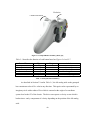
3.3 Gamepad Controls ................................................................................................61
3.4 Encoder Sub-VI .....................................................................................................65
3.5 Desired Pod Angle Sub-VI ....................................................................................68
3.6 Inverse Kinematics Sub-VI ....................................................................................72
3.7 Closed-loop Control System Sub-VI .....................................................................76
3.8 Pod Voltage Control Sub-VI .................................................................................84
Chapter 4 Vehicle Parameterization .................................................................................87
4.1 Modeling Preparation...........................................................................................87
4.2 Tire Model.............................................................................................................87
4.2.1 Rolling Resistance........................................................................................88
4.2.2 Longitudinal Tire Forces .............................................................................89
4.2.3 Lateral Tire Forces ......................................................................................94
4.3 Air Resistance .......................................................................................................97
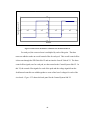
4.4 Closed-loop Motor/Wheel Speed Control Characterization.................................99
4.5 Slip-ring Friction .................................................................................................102
Chapter 5 Simulation and Control ..................................................................................107
5.1 Simulation and Control Overview ......................................................................107
5.2 Control Strategy and Simulation Architecture ...................................................108
5.3 Desired Pod Angles – Setpoint Generation ........................................................112
5.4 Inverse Kinematics Model – Feedforward Control ............................................114
5.5 Pod Control – PID Controller ............................................................................117
5.6 Wheel Speed Model Sub-model – Transfer Functions ........................................122
5.7 Tire Model...........................................................................................................125
5.7.1 Longitudinal Tire Model ............................................................................126
5.7.2 Lateral Tire Model .....................................................................................128
5.7.3 Rolling Resistance......................................................................................129
5.8 Air Drag Model ...................................................................................................130
5.9 ODV Plant Sub-model.........................................................................................132
5.10 Pod Models .......................................................................................................138
Chapter 6 Simulation and Actual Vehicle Comparison ..................................................144
6.1 The Comparison of the Actual ODV to the Simulation .......................................144
6.2 Longitudinal Comparison ...................................................................................145
6.3 User Defined Turn and Vehicle Controller Comparison....................................153
6.4 Test Course Comparison .....................................................................................157
Chapter 7 Project Reflection and Future Work...............................................................164
7.1 Summary of Project.............................................................................................164
7.2 The Progression of the Project ...........................................................................165
7.3 Reflection and Future Builds ..............................................................................167
7.3.1 Build Quality, Manufacturing, and Materials ...........................................167
7.3.2 Motors, Gearboxes, and Batteries .............................................................168
7.3.3 Suspension..................................................................................................170
7.3.4 Slip-rings ....................................................................................................171
7.3.5 Tires and Wheels ........................................................................................171
7.3.6 Simulation and Software ............................................................................172
7.4 Conclusion ..........................................................................................................176
References ........................................................................................................................177
ListofFigures
Figure 1-1 Three-wheeled Omni-directional Vehicle Architecture [2] ...............................6
Figure 1-2 An Example of a Skid-steer Chassis and Drivetrain [6] ....................................8
Figure 1-3 Photos of a Mecanum Wheel [8] ........................................................................9
Figure 1-4: A Sample Vehicle Utilizing the Mecanum Wheel [4] (top) [7] (bottom) .......10
Figure 1-5 Vehicle Architecture and Layout [1]................................................................12
Figure 1-6 The Progression of the ODV at the end of August 2007 [1] ............................14
Figure 1-7 Pod Assembly at the end of August 2007 [1] ..................................................15
Figure 2-1 Approximate Dimensions of the Chassis and Pod ...........................................18
Figure 2-2 CATIA 3D Rendering of the ODV [1] ............................................................19
Figure 2-3 Isometric View of Mechanical Assembly with Body Coordinate Frame [1]...20
Figure 2-4 Front View of Mechanical Assembly with z-axis [1] ......................................20
Figure 2-5 Overall Vehicle Control Block Diagram w/Control System............................23
Figure 2-6 Top-level Vehicle Wiring Schematic ...............................................................25
Figure 2-7 Pod Design and Suspension Layout (suspension movement shown) [1] .........29
Figure 2-8 Completed Pod Assembly ................................................................................30
Figure 2-9 1-Q-EC Amplifier DEC 50/5 Controller [15] ..................................................31
Figure 2-10 Switch Configuration for Speed Control [15] ................................................32
Figure 2-11 EC 45 Flat Brushless Motor [16] ...................................................................34
Figure 2-12 Summary of Data Acquisition Card Pin Layout [17].....................................39
Figure 2-13 DC Motor Pin Layout [16] .............................................................................41
Figure 2-14 Wiring Diagram Between the DC Motor and Controller ...............................41
Figure 2-15 Wiring Set-up Between Data Acquisition Card and Motor Controller ..........42
i Figure 2-16 Wiring Set-up Between Acquisition Card and Encoder ................................42
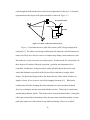
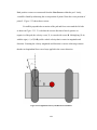
Figure 2-17 Test Experiment for Determining the Moment of Inertia of an Object [18] ..45
Figure 2-18 Xbox 360 Wireless Game Pad [20] ................................................................49
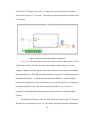
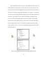
Figure 3-1 Front Panel Screen Shot of the Overall Vehicle VI .........................................53
Figure 3-2 Voltage Circle .................................................................................................54
Figure 3-3 Pod and Wheel Numbering System .................................................................56
Figure 3-4 Overall Vehicle VI Back Panel Summary Block Diagram ..............................58
Figure 3-5 Gamepad VI Back Panel ..................................................................................61
Figure 3-6 Gamepad Button Summary (Front) [20] ..........................................................62
Figure 3-7 Gamepad Button Summary (Back) [21] ..........................................................63
Figure 3-8 Encoder VI Back Panel (Matrix Comparison) .................................................66
Figure 3-9 Encoder VI (Front Panel) .................................................................................68
Figure 3-10 Breakdown of Various Kinematic Inputs on the Vehicle ..............................70
Figure 3-11 The Orientation of Pod Joints in Relation to the Chassis...............................70
Figure 3-12 Desired Pod Angle VI Back Panel (Construction of the N-Matrix
and User Inputs) .................................................................................................................71
Figure 3-13 Desired Pod Angle VI Back Panel (N-Matrix and Pod Angle Output) .........72
Figure 3-14 Pod Geometry Description [1] .......................................................................73
Figure 3-15 Feedforward Control Back Panel (Construction of Equation 3-1).................74
Figure 3-16 Feedforward Control Back Panel (Wheel Voltage Calculation and
Normalization) ...................................................................................................................75
Figure 3-17 PID Gain VI Back Panel ................................................................................77
Figure 3-18 PID Gain VI Back Panel (Error Calculation) .................................................78
Figure 3-19 Control Effort and Direction Sub-VI within the PID Gain Sub-VI ...............79
ii Figure 3-20 Control Effort Calculation as a Function of Calculated Pod Error ................80
Figure 3-21 Direction Calculation as a Function of Calculated Pod Error ........................81
Figure 3-22 Control System VI Back Panel ......................................................................82
Figure 3-23 5-Volt Normalization VI Back Panel .............................................................83
Figure 3-24 Pod Voltage Control Sub-VI Back Panel (Analog Signals)...........................85
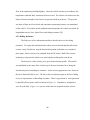
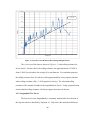
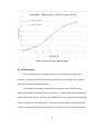
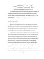
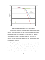
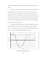
Figure 4-1 Coast-down Test Results for Determining Rolling Resistance ........................89
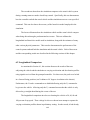
Figure 4-2 Explanation of Variables in Slip Ratio Formula ..............................................90
Figure 4-3 Example Velocity Profile Used to Calculate Slip Ratio ..................................91
Figure 4-4 Slip Ratio versus Accelerating Force ...............................................................92
Figure 4-5 Complete Longitudinal Tire Model .................................................................94
Figure 4-6 Lateral Tire Force Generation ..........................................................................95
Figure 4-7 Experimental Set-up for Measuring Lateral Force...........................................96
Figure 4-8 Lateral Tire Force Data and Model ..................................................................97
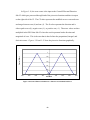
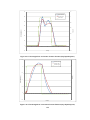
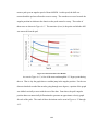
Figure 4-9 1-Volt Straight-Line Acceleration Transfer Function
(Step Input Response) ......................................................................................................100
Figure 4-10 5-Volt Straight-Line Acceleration Transfer Function
(Step Input Response) ......................................................................................................100
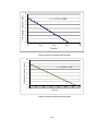
Figure 4-11 Pod Coast-down Test Results.......................................................................103
Figure 4-12 Pod 1 Coast-down Velocity Profile..............................................................104
Figure 4-13 Pod 2 Coast-down Velocity Profile..............................................................104
Figure 4-13 Pod 3 Coast-down Velocity Profile..............................................................105
Figure 5-1 Overall Vehicle Control Block Diagram w/ Control System.........................109
Figure 5-2 Overall Simulation Architecture ....................................................................111
Figure 5-3 M-file Containing all Vehicle Parameters and Characteristics ......................111
iii Figure 5-4 Desired Pod Angle Sub-model Location in the Simulation ...........................113
Figure 5-5 Desired Pod Angles Sub-model Contents ......................................................114
Figure 5-6 Inverse Kinematics Sub-model Location .......................................................115
Figure 5-7 Inverse Kinematics Sub-model ......................................................................116
Figure 5-8 Pod Control Sub-model Location...................................................................117
Figure 5-9 Pod Control Sub-model ..................................................................................118
Figure 5-10 Wheel Voltage Normalization Function ......................................................121
Figure 5-11 Wheel Speed Model Sub-model Location ...................................................122
Figure 5-12 Wheel Dynamics Sub-model Block Diagram ..............................................123
Figure 5-13 Tire Sub-model Locations ............................................................................125
Figure 5-14 Longitudinal Tire Sub-model .......................................................................126
Figure 5-15 Lateral Tire Sub-model ................................................................................128
Figure 5-16 Rolling Resistance Sub-model .....................................................................130
Figure 5-17 Air Resistance Sub-model ............................................................................131
Figure 5-18 Plant Sub-model Location ............................................................................133
Figure 5-19 Summation of Longitudinal Forces within the ODV Plant Sub-model .......134
Figure 5-20 Lateral Tire Force and Pod Location within the Plant Model ......................135
Figure 5-21 Air Resistance Forces and Chassis Location within the
ODV Plant Sub-model .....................................................................................................136
Figure 5-22 Chassis Information Block ...........................................................................137
Figure 5-23 Simulink’s Chassis (blue) and Pod (gray) Graphical Representation ..........138
Figure 5-24 Inside a Pod Sub-model (Planar and Revolute Joints) .................................139
Figure 5-25 Longitudinal Velocity and Direction Calculation ........................................141
iv Figure 5-26 Lateral Slip Angle and Direction Calculation ..............................................143
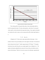
Figure 6-1 1-Volt Acceleration Profile for the Simulation and Actual Vehicle ..............146
Figure 6-2 5-Volt Acceleration Profile for the Simulation and Actual Vehicle ..............147
Figure 6-3 1-Volt Various Acceleration and Deceleration Profile
Comparing the Simulation to the Actual Vehicle ............................................................150
Figure 6-4 2-Volt Acceleration Profile for the Simulation and Actual Vehicle ..............151
Figure 6-5 Commanded Turn Profile Vy = 2V, ω = +0.06 to +0.50 rad/s .....................154
Figure 6-6 Test Course Layout and Desired Path ............................................................157
Figure 6-7 Simulation and Actual Vehicle Turn Command Timing ...............................160
Figure 6-8 Chassis Heading Comparison ........................................................................161
v ListofTables
Table 2-1 Description of Wiring Pathways in Figure 2-6..................................................26
Table 2-2 Motor Pin Summary [16]...................................................................................40
Table 2-3 Summary of Pin Connections Passing through the Slip-rings...........................43
Table 2-4 Summary of Masses and Inertias .......................................................................45
Table 3-1 Gamepad Button Summary ...............................................................................63
Table 5-1 Ziegler-Nichols Method for Tuning Control Gains [28] .................................119
Table 6-1 Command Timing Comparison .......................................................................160
vi 1.Introduction
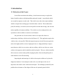
1.1 Motivation of the Project
In an effort to modernize the military, it has become necessary to explore the
limits of mobile robotics with high mobility and speed in mind. A specialized vehicle
was created in response to such a task. This vehicle was to have three major attributes
which set it apart from existing types of mobile robotic vehicles. This includes three
pods (for stability), six wheels (two on each pod for traction and steering), and zero-turn
radius capability (for maneuverability). This vehicle was also configured to be teleoperated as to allow soldiers to remain at a safe distance.
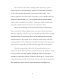
One particular use of such a robotic vehicle is to inspect the chassis or
undercarriage of military vehicles such as the Humvee [1]. This application requires the
vehicle to have a low-profile. While the inspection process in itself does not require the
robot to be highly mobile or to have high speed, there is a high probability to inspect
more than one vehicle in one session, and since military vehicles are driven on various
surfaces, the inspection vehicle should be mobile and quick. This new vehicle should be
able to traverse various terrain profiles ranging anywhere from smooth parking lots to
small obstacles in an off-road setting.
Inspecting the undercarriage of vehicles often requires soldiers to be placed in
dangerous situations. In an attempt to reduce risk, cost, and improve the ease of
inspection, the need for such a vehicle has developed. The challenges presented by this
problem drove the nature of the design of this new tele-operated ground vehicle.
1 Due to the need for the vehicle to be highly mobile and relatively quick, the
vehicle needed to be easily and intuitively controlled. Due to the nature of a soldier’s
job, the vehicle should not be operated by direct contact from the soldier. In this
particular application, the reason a vehicle, such as this, exists is so that the soldier does
not have to be placed in harm’s way. This requirement makes it imperative that the
soldier be able to control the device remotely. Furthermore, a soldier should be able to
pick up the controller and instinctively know how to operate the vehicle.
The uses of the technology are not only limited to military or inspection uses.
This is merely one use of the technology and one area where it has become necessary.
Many other applications exist that require zero-turn radius operations combined with high
amounts of traction. It is not inconceivable to see this technology make its way into
modern lawnmowers, ship container movers, automated vacuum cleaners, and maybe
someday passenger vehicles. This project is still in the early stages of development and
offers a proof of concept and a test bed for which other applications can be explored.
Physically constructing the vehicle allows the opportunity to observe any
unforeseen problems. With only theory or simulation to back up any hypotheses, it could
be easy to overlook even simple problems. Building the vehicle also opens up the
opportunity to explore how the driver will interface with the vehicle. It is now easier to
evaluate the intuitiveness of the vehicle controls. Later, the vehicle may be modified for
fully autonomous control or to test new physical dimensions and configurations.
2 1.2 Motivation and Progression of this Report
The purpose of this document is to explain the development of the Omnidirectional Vehicle (ODV) as it is currently being used. This report explains the physical
layout of the vehicle as well as all of its components. All of this is done in preparation
for the explanation of the control system and overall control strategy used on the vehicle.
The motivation of the project, as mentioned in Section 1.1, only sets a specific need on
the physical requirements of the vehicle. However, it is the control system and strategy,
in conjunction with the mechanical design of the vehicle, that allow the vehicle to
successfully fulfill the goals for which it was designed.
The remainder of Chapter 1 discusses other vehicle architectures that could have
been used and provides reasoning as to why the current architecture was chosen. Chapter
2 provides a breakdown of the physical components of the vehicle and discusses how the
components are physically connected and how they communicate with one another.
Building off of the physical components, Chapter 3 explains the software and how
to control the vehicle. It discusses the LabVIEW programming environment employed
and explain how the software provides overall communication to and from all of the
actuators and sensors on the vehicle. Chapter 3 also begins to give insight into the
vehicle’s overall control strategy.
In Chapter 4, explanations of the vehicle’s physical characteristics are provided.
It covers test methods and results that graphically show how the vehicle accelerates,
decelerates, and maneuvers. This data allows the characterization of physical parameters
such as the dynamics of the electronic motors, the air drag constant for the vehicle, the
3 character of the friction in the slip-rings, and yields an overall picture of the tire
characteristics.
Chapter 5 discusses the simulation environment and how MATLAB and Simulink
are used to simulate the vehicle. Chapter 5 combines the dynamic physical characteristics
of Chapter 4 with the inertias, masses, and dimensions of the components found in
Chapter 2. All of these elements were needed to create a simulation model that could be
useful for testing different vehicle geometries and configurations. The simulation also
provided a test bed to test new control strategies before risking any damage to the
hardware on the actual vehicle.
Chapter 6 compares data from the actual vehicle to results from the simulation.
Several driving test cases have been conducted with the actual vehicle for the purposes of
benchmarking. The trajectory of the chassis, wheel speeds, and control system
effectiveness is compared to the simulation using comparable user inputs. Finally,
Chapter 7 concludes the report and discusses the results from Chapter 6. Additional
information regarding possible directions for future work and reflection on the project as
a whole will be given in this chapter.
1.3 Other Omni-directional Vehicle Architectures
Omni-directional vehicles are a special type of vehicles that allow ground travel
in any direction without the need to rotate the chassis or body. They offer zero-turn
radius capability, thus allowing the vehicle to operate in confined spaces. Most ground
vehicles have a drivetrain type which confines how the vehicle traverses terrain, usually
4 confining the chassis orientation. An Omni-directional vehicle has a drivetrain that
allows the vehicle to travel in any direction and with any chassis orientation.
There are a variety of architectures that allow for zero-turn radius maneuvers; one
of the major design considerations for the project. Each of these approaches offers its
own benefits and drawbacks. A few of these architectures are described in section 1.3.1,
before the specific approach applied in this project is discussed. The specific classes of
omni-directional vehicle that will be discussed are three-pod, skid-steer, four-wheeled,
and vehicles using specialized wheels. The architecture employed in this project is
compared and contrasted to these other known techniques.
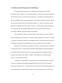
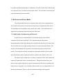
1.3.1 Three-pod Designs
The three-pod designs utilize six motors, and are commonly broken down into
two variations. In one variation, each pod contains one wheel and one motor to control
the vehicle’s velocity. A separate steering motor is used to control the orientation of each
pod [2] [3]. Figure 1-1 shows an example of a three-wheeled, three-pod omni-directional
architecture.
5 Figure 1-1 Three-wheeled Omni-directional Vehicle Architecture [2]
The architecture presented in this document shows that the same number of
motors (six motors) can utilized in a different way than the three-pod, three-wheeled
omni-directional architecture. Six motors are now used to propel the vehicle rather than
reserving three solely for the purposes of steering the vehicle. It uses six wheels rather
than three, and the steering is achieved by a difference of velocity between the right and
left wheels on each of the pods.
An advantage of having six wheels on the ground, rather than three, is that it
increases the maximum force that can be applied at the ground/tire interface and in turn
increases the speeds that can be achieved. The vehicle architecture presented will be
discussed in further detail in Section 1.4.
6 1.3.2 Skid-steer Designs
Skid-steer vehicles, similar to a tank, offer zero-turn radius capability. They have
a chassis which is supported by wheels or a track system. The wheels or tracks are laid
out similar to that of a passenger vehicle. Though the vehicle may look similar to a
passenger vehicle in terms of drivetrain, it does not steer in the same fashion. The wheels
or tracks are aligned in parallel with the chassis’s intended direction and never change
their angle in relation to the chassis. The vehicle is able to steer or change direction due
to a velocity difference between the right and left wheel sets or track systems [4] [5].
The pod structure, as described in this document, utilized the ability to control a
velocity difference between the right and left wheels. This orientation method will
directly control the direction of the pods and indirectly control the orientation of the
vehicle’s chassis.
This method proves very effective for rotating the chassis especially where a zeroturn radius is necessary. It is very simple to implement mechanically, and is relatively
simple to implement from control a control standpoint.
The traditional application of skid-steer was not chosen for this project because
zero-turn radius is not the only requirement of the vehicle. The orientation of the chassis
is something that also needs to be controlled, either to maneuver the vehicle around, or to
point a particular part of the vehicle in a certain direction. Many applications, besides
vehicle undercarriage inspection, could require control of the orientation of the chassis.
For instance, large cargo containers aboard a cargo ship could require an omni-directional
vehicle which could perform strafe maneuvers without changing the orientation of the
cargo. A skid-steer vehicle cannot perform this function simply because the wheels
7 cannot be oriented in relation to the chassis. Therefore, the direction of motion of the
wheels always forces the front of the chassis in the same direction. An example of a
skid-steer vehicle is shown in Figure 1-2.
Figure 1-2 An Example of a Skid-steer Chassis and Drivetrain [6]
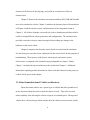
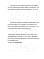
1.3.3 Special Wheel Types
Other types of omni-directional vehicles have a drivetrain that look very similar to
that of the skid-steer type vehicles. Like the skid-steer vehicles, the wheels never change
their angle in relation to the chassis. Instead, they employ specialized wheels, such as the
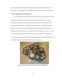
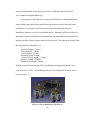
mecanum wheel, to do all of the turning and chassis orientation [4] [7]. Figure 1-3 shows
an example of a mecanum wheel.
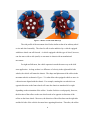
8 Figure 1-3 Photos of a Mecanum Wheel [8]
The side profile of the mecanum wheel looks similar to that of an ordinary wheel
or tire and wheel assembly. The wheel is still circular and this why a vehicle equipped
with these wheels can roll forward. A vehicle equipped with this type of wheel, however,
can also move side-to-side (strafe) or can rotate its chassis with no translational
movement.
For right and left turns, the vehicle operates in much the same way as the skid
steer application. As long as there is a difference of velocity in the right and left side
wheels, the vehicle will rotate the chassis. The shape and placement of the rollers in the
mecanum wheels as shown in Figure 1-3 is what allows the equipped vehicle to move in
a direction not aligned with the chassis. For example, rotating the rear wheels in an
opposite direction to the front wheels will cause the chassis to translate left or right
depending on the orientation of the rollers. In order for this to work properly, however,
the direction of the rollers on the rear wheels need to be opposite in direction of the
rollers on the front wheels. Moreover, the direction of the rollers between the right side
and the left side of the vehicle also must have opposing directions. Therefore, the rollers
9 on the left front and right rear will be facing the same direction, and the rollers on the
right front and left rear will be facing the same direction. Figure 1-4 shows a vehicle
layout using the mecanum wheels.
Figure 1-4 A Sample Vehicle Utilizing the Mecanum Wheel [4] (top) [7] (bottom)
Though this layout proves to be very advantageous for control of vehicle
orientation and translational movement, there are some drawbacks. This architecture
type does not lend itself well for the overall efficiency of the vehicle. For the same
reasons that the mecanum wheels are advantageous, they are also inefficient. This is due
in part because the wheel is always exerting a force perpendicular to the direction of
travel as well as parallel to the direction of travel. When the vehicle is utilized for only a
single direction of travel, only one component of the force generated by the wheel is used
10 to move the vehicle. Since the rest of the forces generated by the wheels are opposing
one another, the vehicle is wasting energy only to keep itself stabilized.
Yet another disadvantage is that the vehicle using these wheels can only be used
on certain surfaces. The wheels and tread surfaces are usually constructed of relatively
hard materials such as plastics. This offers little compliance to any disturbance presented
by the surface that the vehicle is trying to traverse. The standard pneumatic tire offers the
ability to maintain a tractive force even over small obstacles or debris [3] [9].
The shape of the mecanum wheel also prevents off road use and, therefore, is
usually restricted to use on flat terrain. The reason the wheels need flat terrain is so that
the road is always ensured to come in contact with the center of the wheel. If the wheel
contacts the road surface at the side wall or the side of the rollers, the entire mechanism
for which the wheels are able to work is no longer present. This situation changes the
direction and magnitude of the forces generated by the wheels which will induce an
undesired moment on the chassis. It is the balance of forces on the chassis which keep
the chassis orientated as desired. Once this balance is disturbed by an off-cambered
surface, the control system and/or the user would lack the ability to maintain proper
control of the vehicle. Due to the possible application of the proposed vehicle to different
terrains, this type of architecture was not chosen for this project [3] [10].
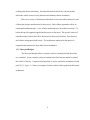
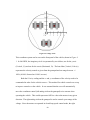
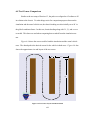
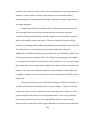
1.4 Omni-directional Vehicle Architecture Used in this Project
The architecture chosen for the vehicle used in this project, as mentioned
previously, consists of three pods, each of which includes two independently driven
wheels. Each wheel is driven by its own motor and the vehicle is steered by orienting the
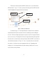
11 pods through the differential motion of the left and right wheels of the pod. A schematic
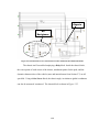
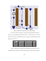
representation of the layout of the pods and wheels is shown in Figure 1-5.
Conventional wheels
Vehicle Chassis
Hinge joint
Split D
Offset S
Figure 1-5 Vehicle Architecture and Layout [1]
Figure 1-5 represents the active split offset castor (ASOC) design employed for
each pod [11]. The offset castor design (with distance S) makes the vehicle holonomic in
nature (less likely for a wheel to come to a complete stop during various maneuvers) and
thus makes it is easier to traverse curved trajectories. In other words, the castor allows all
three degrees of freedom of the pod (x-position, y-position, and orientation) to be
controlled. Furthermore, using two wheels with a split (D) reduces the load on each
wheel and eliminates a great deal of the frictional forces inherent in a single wheel
design. The dual wheel design reduces the chance that one of the wheels will have an
angular velocity of zero (come to rest) while changing directions [11]. Wheels that
continuously roll while changing directions maintain lower and consistent frictional
forces by avoiding the stiction associated with the rest state. This leads to a much more
smooth and predictable vehicle. This design can be seen on modern airliners. Having the
offset split castored wheel mechanism alone does not ensure omni-directionality as some
paths may require one of the wheels to stop while reorienting. However, an ASOC
12 design in conjunction with controlling the velocity of each wheel, any position and
orientation of the hinge joint can be achieved. Allowing the joint to move
instantaneously in any direction and orientation is the primary function of the ASOC
design and is what makes the vehicle omni-directional [11].
The ASOC design allows the vehicle to be oriented independent of its direction of
motion as opposed to more traditional skid-steered vehicles. Furthermore, this
architecture allows for the generation of higher traction forces and the achievement of
greater translational speed than other three-pod architectures due to the fact that six
driven wheels are in contact with the ground, rather than only three. Also, this
architecture also is more efficient than architectures that rely on mecanum wheels and
allows for operation across a variety of terrains, which is not possible with mecanum
wheels.
One possible disadvantage of the chosen architecture is that the control strategy
that must be employed may be more complicated than required with other architectures.
During development it was found that the vehicle could not be driven at high-speeds
using an open-loop, kinematics-based control strategy and a dynamic controller needed to
be designed and implemented. Specifically, the control strategy was designed to help the
driver maintain the desired direction of motion and orientation of the vehicle in the
presence of road disturbances or significant wheel slippage and scrubbing.
This section of the report introduced some examples of various types of
architectures for omni-directional vehicles and explained the reasoning by which the
ASOC architecture was chosen. It is, however, conceded that architectures other than
13 those considered here may have advantages and could be explored in the future. The
architecture of this particular vehicle will be further explained and explored in Chapter 2.
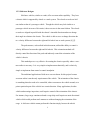
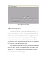
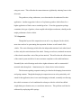
1.5 The Progression of the Project The construction of the vehicle chassis and drivetrain took place between January
and August of 2007 by the senior mechanical engineering design class. All of the
mechanical design was done by students enrolled in that class as well as most of the
manufacturing and assembly. They did not finish the project as this project provided
ample work for several semesters. Regardless, the work they did represented a great
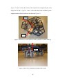
challenge for the senior design class and served well as a final project. Figures 1-6 and
1-7 show the results of the work done by the senior class of 2007, as of August 2007.
One can see that the students back in 2007 had completed the mechanical assembly of the
pod and the chassis, and installed the batteries and encoders [1].
Figure 1-6 The Progression of the ODV at the end of August 2007 [1]
14 Figure 1-7 Pod Assembly at the end of August 2007 [1]
The remainder of the manufacturing, assembly, wiring, and computer control
became a separate project since these three aspects became part of the overall control
strategy. The slip-rings, allowing full electrical connectivity throughout a 360 degree
rotation, represented the last of the major sub-assemblies. All other items related to the
completion of the vehicle were a matter of preference on placement and did not influence
the performance of the vehicle.
The choice of signals to include in the data acquisition and the hardware
associated with the overall control of the vehicle aided in clarifying the final layout of the
vehicle. For example, the data acquisition cards were one type of component that placed
limitations on the way the vehicle was wired. The limitations on the number of available
data acquisition channels forced a choice between the features that made it onto the
vehicle and those that did not. Limitations such as these are what resulted in the final
configuration and capabilities of the vehicle. Placement of the data acquisition boxes,
motor controllers, wire routing and battery connections were all set as necessary to
15 provide the proper function of the vehicle. The wiring was kept as short as possible
while trying to maintain a simple layout to the components.
The remaining items assembled onto the vehicle were not critical to the larger
design of the vehicle, but were necessary for its function. The encoders, pulleys on the
encoders and pods, belts, belt tensioners, and miscellaneous bracketry represented the last
of the mechanical assembly.
The battery connectors and wires were soldered together to allow power to the
vehicle. Three wire and connector assemblies, one for each battery, were needed which
were later installed into the floor pan. The gearboxes for the electric motors also
provided a small hurdle which required machining work. One of the gears inside each
gearbox was plastic and had to be switched out for a metal gear in order to ensure
durability. Later, a flat surface was machined into the output shafts of the gear boxes.
The flat surface provided flat spots needed for set screws needed to couple the gear boxes
to the wheel axles.
Once the machine work and assembly was completed, the controls aspect of the
project could be developed. A laptop equipped with LabVIEW served as the interface
between the hardware that physically actuates and senses the vehicle and the software
that controls how the hardware operates.
Although there were several control strategies that could be studied, not all were
explored. The reasons for this are time, manpower, money, and the current state of the
vehicle. The goal was simply to get the vehicle to work well enough to achieve the given
operational requirements so that the vehicle could be employed as a proof of concept.
For these reasons, control at the pod level was the avenue chosen. Control at the vehicle
16 level was one choice considered, but the vehicle had an emphasis on speed and reaction
time. With these requirements, a pod-level approach to control was deemed better in
comparison to vehicle-level approach to control.
Since the pods are smaller and have less inertia than the overall chassis, the pods
should conceivably be quicker to respond to inputs from both the operator and the control
system. The pods are closer to the point where the forces are actually generated, at the
wheel, therefore, there are fewer dynamics between what is being controlled and the
actuation being employed to achieve the desired control. Furthermore, vehicle-level
control would require the use of an inertial sensor, which is potentially expensive. While
it is ultimately the goal to control the motion of the vehicle as a whole, the driver is still
in the loop to assist with this and the pod-level control is there just to assist the driver.
Additional iterations of control for this vehicle may very well employ vehicle attitude
control through the use of an inertial measuring unit (IMU) which measures vehicle
heading. Once both control systems (pod level and vehicle level) are studied, tested, and
calibrated, it would be conceivable to place them both on the vehicle. This would
provide control at both the pod-level and vehicle-level. Ideally, both systems would
provide complementary aspects to the control, the pod-level providing quick response to
commands and disturbances and the vehicle-level maintaining the ultimate goal of
controlling vehicle attitude
17 2.HardwareIdentificationandSet‐up
2.1 Vehicle Design and Architecture
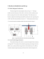
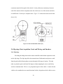
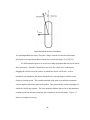
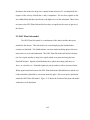
The basic design of the chassis and pod is shown in Figure 2-1. This figure
includes some basic dimensions of the vehicle as well as the vehicle coordinate system
that were employed in the vehicle software and simulation. These dimensions were
based on a Quality Functional Deployment (QFD) created by the senior engineering class
of 2007 and will be discussed further in Section 2.1.1. The dimensions shown in Figure
2-1 are also relevant to the simulation which is discussed in detail in Chapter 5.
Figure 2-1 Approximate Dimensions of the Chassis (left) and Pod (right)
2.1.1 Overall Vehicle Design (Mechanical)
The mechanical design of the vehicle was started and completed between January
and August 2007. The students of the mechanical engineering senior design class used a
QFD to come up with specification targets that the vehicle should meet [12]. QFD is a
commonly employed engineering design tool that aids in the initial development of a
18 product. Further details of the QFD process can be found in the tutorial shown at
www.webducate.net/qfd/qfd.html [12].
As is practice in the QFD process, target specifications were benchmarked from
other existing robots that perform similar function to those desired of the robot under
consideration. An analysis of the priorities of the robot helps decide the major
dimensions, materials, cost, and overall performance. Although a QFD was utilized for
this project, further consideration of the dimensions and performance characteristics was
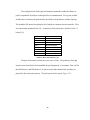
taken as needed to allow for better control over the vehicle. The main specifications from
the initial QFD are listed below [1].
o
o
o
o
o
o
o
Ground clearance: 4 inches
Wheel diameter: 7 inches
Caster distance: 0.5 inch
Maximum speed: 10 mph
Center of Gravity height: 3.5 inches
Height of vehicle: 12 inches
Maximum step height: 2 inches
With the main specifications listed above, preliminary renderings and sketches were
completed with CATIA, a 3D modeling software. The resulting CAD model is shown
below in Figure 2-2
Figure 2-2 CATIA 3D Rendering of the ODV [1]
19 Figures 2-3 and 2-4, show the results of the construction as completed by the senior
design class of 2007. Figures 2-3 and 2-4 shows the body-fixed coordinate system
employed on the vehicle which was also shown in Figure 2-1.
x-axis
y-axis
Figure 2-3 Isometric View of Mechanical Assembly with Body Coordinate Frame [1]
z-axis
Figure 2-4 Front View of Mechanical Assembly with z-axis [1]
20 This document concentrates primarily on the dynamic modeling and control of the
vehicle as it was received. Physical dimensions of the device itself including parameters,
such as caster offset, all affect the control design and ultimately the control gains.
Although the structure of the control strategy does not change with varying the physical
dimensions of the vehicle, the control effort and control timing would have to be recalibrated to suit the new physical parameters.
For example, caster distance and pod spacing can have a great effect on the
control design. Decreasing the caster distance or offset will make it easier for the vehicle
to complete turns. The pods require less net torque from the motors to complete turns
and the lower offset also makes the pods respond quicker to inputs. Increasing the caster
offset makes the opposite true. The vehicle will become more stable while traversing in a
straight line, but it will make turns more difficult to complete.
Finding the appropriate amount of caster offset, wheel spacing, and pod spacing is
a balancing act that depends on requirements from the user. No one particular value is a
necessity or a direct requirement for the proper operation of the vehicle. Picking these
values is a result of a study done outside of this project and, therefore, is beyond the
scope of this document.
Physical parameters such as ground clearance, center of gravity height and ground
clearance are parameters chosen to be specific for the vehicle’s use. The ground
clearance is chosen to ensure the vehicle can clear certain size obstacles that could be
present on the surfaces on which a soldier decides to operate the vehicle. The vehicle is
designed to be operated in urban and desert environments. In these environments, it is
21 not expected to come across obstacles that are taller than an average red brick lying on its
side.
The overall height and center of gravity height along with overall width of the
vehicle go hand in hand with each other. The maximum height of the vehicle was chosen
as an acceptable height which could still roll under the military Humvee having a
standard ride height of around 16 inches [13] [14]. The extra space could serve as a
safety factor for approach and departure angles that could be an obstacle offered by the
terrain.
A lower center of gravity height is better for the rollover performance and weight
transfer of the vehicle. Unfortunately, it is difficult to keep center of gravity height low
with a project that is also dependent on ride height clearance. The center of gravity
height is greatly dependent on the items attached to the chassis that often times cannot be
avoided. The items on the vehicle are necessary for the proper function of the vehicle
and so decreasing weight in one area and adding it in another is not always easy. Instead,
the mounting location for each component was kept as low as possible in the chassis in an
attempt to reduce the height of the center of gravity. For example, the batteries, which
are among the heaviest and most dense components, are mounted to the floor pan of the
vehicle.
Other dimensions like wheel diameter were chosen based on their effect on other
key parameters while keeping cost in mind. The wheels could be considered off-the-shelf
items thereby reducing cost. Therefore, picking a wheel size was done by picking one
that will give the vehicle the ride height it needs, allows the vehicle drive over obstacles,
and maintain a standard wheel size.
22 2.1.2 Overall Vehicle Design (Control)
This section touches briefly on the control strategy used on the vehicle and the
ways that the hardware carries out the demands of the control system. The control
system, from the software point of view, will be discussed in more depth in Chapters 3
and 5. Chapter 3 discusses the architecture of the software (LabVIEW) and the control
system programming which in turn instruct the hardware. Chapter 5 discusses the
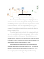
architecture of the control system as it pertains to the simulation. The control strategy
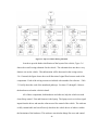
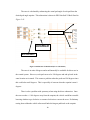
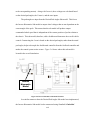
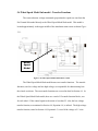
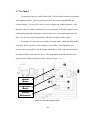
from here forward follows the structure laid out in Figure 2-5. Keeping this figure in
mind may prove helpful as one considers the actual hardware and software on board the
vehicle.
Figure 2-5 Overall Vehicle Control Block Diagram w/Control System
The initial inputs from the user are the vehicle’s desired translational velocity (xand y-components) and its desired angular velocity. From experience it has been
determined that a kinematics-based open-loop control system is insufficient to allow an
operator to drive the vehicle at even moderate speeds. Specifically, the human in the loop
is sufficient to achieve a desired velocity magnitude, but the slippage and scrubbing
experienced by each of the six wheels makes achieving a commanded direction
impossible at all but the slowest speeds without feedback. Therefore, the control strategy
depicted in Figure 2-5 has been adopted. This strategy attempts to control the orientation
23 of the individual pods as a means for achieving an orientation of the overall vehicle. The
speed control of the wheels themselves is implemented by the motor controllers which
were bought off-the-shelf.
The pod-control strategy specifically attempts to control the angle of a pod with
respect to the chassis. A benefit of this approach is that there is no need to know the
orientation of the chassis which would require a potentially expensive inertial sensor.
Also, the pods will respond much more quickly to control system inputs since they are
closer to the application of the control forces and since the inertia of a single pod is
significantly lower than that of the entire vehicle. The control strategy includes a
feedforward component based on the vehicle kinematics as well as a feedback component
that is based on the error between the commanded and actual pod angle. Each component
of the control has a complementary effect. The feedforward portion of the control has no
dynamics and, as a result, is very fast. Also, since the overall dynamic relations are
nonlinear, the feedforward term is expected to get the output close to the command so
that for small errors, the system behaves approximately linearly. The drawback of the
feedforward control is that it does not account for errors in the model and disturbances,
specifically which come from the slipping and scrubbing of the tires. These errors and
uncertainties are, therefore, corrected for by the feedback portion of the control. The
feedback portion is implemented as a dynamic PID controller which is more robust, but
slower than the feedforward controller. Recall that further details concerning this control
strategy are discussed in Chapter 3 and Chapter 5.
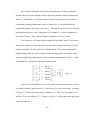
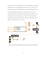
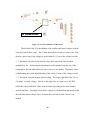
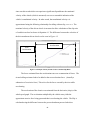
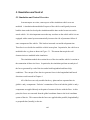
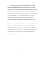
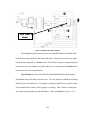
The overall vehicle system is made up of several smaller components that help the
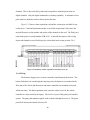
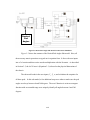
vehicle run as the user wishes. This is depicted in Figure 2-6.
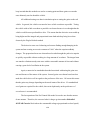
24 Figure 2-6 Top-level Vehicle Wiring Schematic
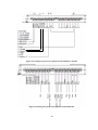
In order to provide further clarification of the layout of the vehicle, Figure 2-6
shows the overall wiring schematic for the vehicle. The schematic does not show every
distinct wire on the vehicle. That information will be discussed in the wiring section,
2.6.4. Instead, the figure shows the overall direction of signal flow between each of the
components. Each of the wiring avenues are labeled with a number for reference. Table
2-1 briefly describes each of the numbered pathways. Sections 2.3 through 2.6 discuss
the hardware used on the vehicle in detail.
All of these components, both hardware and software, help the vehicle run with
closed-loop control. First and foremost is the laptop. The laptop receives wireless signal
inputs from the driver and runs the software used for control of the vehicle. The software
is fully customizable and can effectively alter how the vehicle drives or behaves within
the limitations of the hardware. This software can calculate things like error and control
25 effort, monitor current vehicle status such as individual wheel speeds, and send out
control signals to the motors such as a voltage, direction, or disable commands.
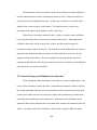
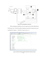
1
2
3
4
5
6
7
8
9
Signals calculated using LabVIEW, as a result of user inputs or vehicle feedback, are sent
to the DAQ cards
Signals from the encoder are sent to the DAQ cards. These signals help track the angular
position of the pods
Motor voltage, disable, and direction signals are sent from the DAQ cards to the slip-rings.
Power supplied by the batteries is also routed through the slip-rings.
Hall-effect sensor counter signals are sent from the slip-rings to the DAQ cards. These
signals help track wheel angular velocity and angular acceleration
Motor voltage (speed command), disable, and direction signals come through the slip-rings
and to the motor controllers. Battery power supply wires are routed from the slip-rings to
the motor controller
The motor controllers send a pulse train from the Hall-effect sensors to the slip-rings
Closed-loop voltage commands are sent from the motor controller to the brushless DC
motors. This voltage physically drives the motors
Pulse trains generated by the Hall-effect sensors are tracked by the motor controllers
Communication signals translated by the DAQ cards from physical signals are sent back to
the computer. LabVIEW processes these signals and uses them for future calculations
Table 2-1 Description of Wiring Pathways in Figure 2-6
The data acquisition cards, which are connected to the computer via USB, send
and receive communication signals given by the software. They serve as the interface
between the software and the sensors and actuators on the vehicle. For this vehicle, the
data acquisition cards will send desired wheel speed, direction, and disable commands to
the motor controllers. They receive an encoder signal which is the angle of the pod in
relation to the chassis. Lastly, they receive counter signals from the Hall-effect sensors in
the motors. This counter signal can be used to calculate actual wheel speeds
The wires running from the encoders to the data acquisition cards are one piece
and do not pass through the slip-rings since both data acquisition cards and the encoders
are attached to the chassis (not the pods). Wires running from the data acquisition cards
and going to the motor controllers must first pass through the slip-rings. This is because
26 the motor controllers are attached to the top faces of the pods which must be able to
rotate through a full rotation.
The motor controllers receive the desired wheel speed, direction, and disable
commands from the laptop through the data acquisition cards. The controllers also
receive data from the Hall-effect sensors in the motors. Based on the angular speed of
the motors, the voltage command from the laptop (which can represent desired speed or
torque), and disable command, the motor controllers controls the motor’s acceleration or
deceleration. It does this since the motor controller will be run in closed-loop speed
control mode. More information on the modes will be given in Section 2.4.
The encoders are attached to the frame or chassis of the vehicle and have a pulley
attached to the input shaft. At the top of the pod is another pulley. The pulley ratio
between the encoder and the pod is 1:1 which will allow direct angular rotation tracking
of the pod in relation to the chassis. The encoders help to track error in the control
algorithm and, therefore, are instrumental in the control of the vehicle.
The motors are DC brushless and are the last element on the vehicle to receive
signals. They operate purely on three voltage excitation signals, one for each of the three
motor windings. The motors also have three Hall-effect sensors which output a pulse
train where each pulse represents an incremental change in motor shaft position. The
motors can be commanded to operate in reverse, and by observing the relative phase of
each of the Hall-effect sensor outputs the direction of motion of the motors can be sensed.
Although the Hall-effect sensors output only position of a motor shaft, the speed of a
motor can be calculated with known elapsed time and the angular position signal. In other
words, the frequency of the pulse train indicates angular speed.
27 2.2 Chassis
There were several limitations handed out to the initial student design team when
designing the vehicle. These limitations drove considerations like the choice of materials
utilized on the vehicle. Steel was chosen as the material for the construction of the
chassis since it is cheap while still maintaining a fair amount of rigidity. Lastly, students
are typically new to manufacturing and activities such as welding. Steel is one of the
easier materials to weld together and provides a good testing ground for students to
practice. In short, it is a good all-around material for a structural application like this.
Other materials such as titanium, aluminum, or carbon fiber could have been used to cut
down on mass, but they come at a greater cost to the consumer. These materials are also
more difficult to employ for construction. Carbon fiber in particular has to be molded
and requires special consideration to the direction and placement of the fibers. Future
iterations of the vehicle may explore the use of these other materials in order to take
advantage of their mass advantage.
The overall layout of the chassis is such that it allows three pods set 120 degrees
apart. The overall dimensions of the chassis are driven by the features needed for the
vehicle. It leaves just enough space for things such as the pods, slip-rings, encoders,
laptop, data acquisition cards, and batteries. Other features such as cameras could be
added, but likely would need to be added to a separately built stage. For now, this
vehicle serves as a proof of concept.
28 2.3 Pod Design
The structure and layout of each pod were chosen as to allow independent vertical
movement between the wheels. An independent suspension was chosen since it allows
better traction and control over the position of the pod. If a solid type axle had been used
between the wheels, there would have been a potential for one of the wheels to lose
traction over uneven terrain. Complete loss of traction on just one of the wheels would
prevent the pod from being able to effectively steer. Furthermore, losing traction on one
or more of the wheels reduces the amount of power that can be applied to the ground and,
therefore, will reduce velocity and or acceleration of the vehicle. Lastly, if the power
cannot be effectively transmitted to the ground, then the control system will not be able to
work as designed. A sketch of the suspension and pod design that illustrates how the
wheels can move independently of one another is shown below in Figure 2-7.
Figure 2-7 Pod Design and Suspension Layout (suspension movement shown) [1]
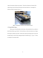
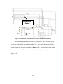
Figure 2-8 shows the actual pod assembly and references the “U” shape, Wheel Bearings,
Top Face, and Motor Controllers.
29 Motor Controllers
Slip-rings
Top Face
Motors
“U” Shape
Wheel Bearings
Center Post
Figure 2-8 Completed Pod Assembly
The center post of the pod is constructed of steel with two linear bearing tracks
mounted on either side. Mounted to the bearing tracks are three aluminum plates
assembled in a “U” shape. Either side of the “U” serves as a mounting point for the
wheel’s axle shaft and bearings. The aluminum plate closest to the center post is
mounted to the linear bearing. It is this linear bearing that allows vertical movement
between the aluminum plates and the steel center post.
The center of the axle is drilled out to allow the gearbox and motor assembly to
couple with the axle. A set screw within the wheel axle prevents any angular slip
between the wheel axle and the gearbox shaft. The gearbox also mounts to an aluminum
plate which in turn mounts to the outer side of the “U”. The motor mounts to the
opposite side of the gearbox and completes the motor and gearbox assembly.
The top face of the “U” shapes serve as mounting locations for the motor
controllers. Each motor controller is secured to the top of the “U” shape with Velcro.
This allows a cost effective and easy mounting structure for the controllers.
30 2.4 Motor Controllers
The motor controllers relay information and control signals between the data
acquisition cards and the motors. They receive the motor control signals including an
analog speed or torque command, as well as a disable and direction bit. The various
potentiometers and switches on the controller can alter control modes, top speed, and
acceleration profiles of the motors and ultimately the vehicle. The controllers also read
the motor Hall-effect sensors for the purposes of closed-loop control and transmit these
signals so that they can be used outside of the motor controllers.
There are three Hall-effect sensors which track the position of the motor shafts.
Utilizing three of the Hall-effect sensors yields higher fidelity than using just one or two.
Observing the phase between multiple Hall-effect sensors also allows determination of a
motor’s direction of motion. Figure 2-9 shows the controller used on the vehicle.
Figure 2-9 1-Q-EC Amplifier DEC 50/5 Controller [15]
31 The controllers are manufactured by Maxon and offer three modes of operation
which include open-loop speed control, closed-loop speed control, and current control
(torque control).
A speed control mode was chosen because it aligns with the commands being sent
to the vehicle by the user (translational and angular velocity). More specifically, closedloop speed control was chosen versus open-loop speed control because it is more robust
to disturbances and to variation amongst the different motors. Torque control was not
selected since it was difficult to command a given velocity. Instead, torque control only
commands the torque output to the wheels. While torque control provides consistent
acceleration profiles on one surface, it does not do so across different surfaces. Closedloop speed control will maintain consistent performance for a variety of surfaces within
reason. Consistent performance makes the vehicle more predictable to the user and easier
to model by simulation. This mode can be set by adjusting the six switches on the
controller. The switch configuration is shown in Figure 2-10.
Figure 2-10 Switch Configuration for Speed Control [15]
Although the above diagram shows the controller setting for the speed control
operation of the brushless DC motor, the user can also adjust switches 2, 5, and 6. The
number 2 switch controls the gain of the motor with the off position being the highest
gain. The gain controls how the vehicle accelerates. The higher the gain, the quicker the
vehicle will reach top speed. The top speed will remain the same no matter which
position the gain is set. The number 5 and 6 switches control the top speed of the motor.
32 These switches can do this as they control the maximum allowable RPM. The highest
speed the motor can attain is achieved by setting switches 5 and 6 to the off position.
Acceleration profiles, top speed, and available torque are all parameters of the
motor that can be adjusted by the potentiometers on the controller. Depending on which
mode the controller is in affects which potentiometer becomes active. For instance, when
in closed-loop speed control mode, the gain potentiometer becomes active. This
potentiometer is able to change how the vehicle accelerates [15].
2.5 Maxon EC 45 Flat Motors
Providing the power and steering capabilities of the vehicle are the six brushless
DC motors. Two motors, one on each side of the pod, connect to the drive wheels and
ultimately allow for translational and rotational movement of the pods. By providing the
same voltage and direction to the motors, they will move the pod in only a translational
direction. A difference in the voltages supplied to the motors can result in either pure
rotation or a combination of rotational and translational movement. Pure rotation will
result if the voltages supplied to the motors are equal in magnitude but in opposite
directions. Voltages in the same direction but different in magnitude will result in both
translational and rotational movement of the pods. It is the control of these scenarios that
move the individual pods that in turn result in the desired movement of the chassis.
The DC motors are also manufactured by Maxon, each produces approximately
50 Watts of power. The particular motors used are the EC 45 Flat Brushless Motor
models. Each motor has three windings and three Hall-effect sensors. Hall-effect
sensors allow the angular displacement of the motors to be tracked and thus allows for
33 consistent control of the speed of the vehicle. It also yields more consistency between
each of the motors which is important since the vehicle uses six of the motors and relies
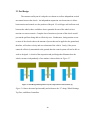
on a difference of velocity to complete turns. Figure 2-11 shows the motors used on the
device [16].
Figure 2-11 EC 45 Flat Brushless Motor [16]
2.6 Slip-rings, Data Acquisition Cards and Wiring, and Encoders
2.6.1 Slip-rings
Providing the bridge between the motor controllers and the data acquisition cards
are the slip-rings. The slip-rings allow the transmission of information and power to and
from the pods while allowing them to rotate through a full range of motion. The only
other way that the pods could turn 360 degrees without tangling the wires would be by
wireless communication. This is a very important aspect for the vehicle. In order for this
vehicle to be considered a true omni-directional vehicle, the pods need to be able to move
34 through 360 degrees of rotation. This prevents the vehicle from getting stuck in tight
surroundings and allows it to maneuver through difficult areas.
There is one slip-ring, shown in Figure 2-8, located at the top of each pod and
each is constructed out of circular shaped aluminum plates. Sandwiched between the
aluminum plates are two circuit board-like circular structures. These circular circuit
board-like structures are what allow electrical connection throughout a 360 degree
rotation of the plates relative to each other.
Molded into the bottom circuit board are 16 brass rings thus allowing 16 separate
electrical signals. The top circuit board remains stationary relative to the chassis and
contains gold leaves which provide the physical connection to the bottom 16 rings
directly below. These gold leaves are shaped like a “V” and are fairly flexible. The
flexibility and shape of the leaves generate a spring force that keeps the connection
between the top and lower plates. Even if the gap between the plates were to vary, the
spring force in the leaves maintains the electrical connection. A circular piece of vinyl,
with a sticky back, was cut out and placed between each of the rotating aluminum plates
and the corresponding circuit-board. This was done to prevent the aluminum plates from
causing a short across different channels of the circuit boards.
After installing the slip-rings, the pods could then be put into their respective
places in the framework. Here, the location of the lower half of the slip-ring becomes
important as this is what can either create or break the electrical connection in the sliprings. If the gap between the plates of the slip-rings is too large, the electrical
connectivity could be affected. Similarly, if the gap is too small, there is increased
35 friction and a risk of breaking the gold tabs. Breaking the tabs off of the slip-rings will
result in a loss of electrical connection.
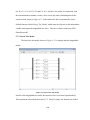
2.6.2 Encoders
The optical encoders, belts and pulleys are connected to the top side of the
vehicle. The pod encoders generate an output that is similar to that produced by the Halleffect sensors but are unable to determine the angular position. The angular position of
an encoder can be determined using a system of wires that switch between high and low
voltage signals. The low voltage is considered to have a value of zero (0), while the high
voltage has a value of one (1). The encoders specifically are 10-bit (employ 10-wires)
such that each revolution can be split into 210 increments. By comparing the string of
values being generated by an encoder to a matrix of combinations of zeros and ones, a
specially written VI can output the current angular position of a pod.
For packaging reasons, each of the encoders is attached to the pods by way of a
belt and pulley mechanism. In order to make the software run correctly and easier to
implement, there had to be a one-to-one ratio between the encoder pulley and the pulley
on the pod. This ensures that the encoders properly track any movement of the pods.
This is very important for the control strategy of the vehicle. Once the pulleys were on,
they were adjusted so that all the pods had a consistent origin.
If a theoretical coordinate system were placed at the center of gravity of the
chassis, shown in Figures 2-3 and 2-4, the positive y-axis would point at the front of the
vehicle. The positive x-axis would point from the right side of the vehicle. The positive
x-axis is synonymous with a pod angle measurement of zero (0) radians, in relation to the
chassis (as read from the encoders). The pods were initially aligned so that the wheels of
36 each pod are facing forward when they are parallel with the positive y-axis thus making
the pods have an angle of π/2 radians in relation to the chassis. This is the default
forward direction as used by the mathematics in the software.
For stability purposes, the front of the vehicle was taken to be one of the flat faces
of the framework. This means that two pods will be leading rather than trailing. It is
believed, however, that the vehicle may be more maneuverable if two of the pods are
trailing.
The encoders were mounted to a special plate which can slide in relation to the
chassis. The mounting plates enable the tension to be properly set on the belt running
between each of the encoders and pods. The remaining hardware is the data acquisition
cards. These were placed on the lower plane of the chassis with Velcro and labeled
corresponding to their respective pods.
The batteries were similarly set in the floor pan of the vehicle. All three wire sets
carrying power to each of the pods had to have their wires soldered into a plug-in
connection. A fuse was introduced in line with the wiring between the motor controller
and the battery to protect against the possibility of over-current or over-voltage. Three
brackets were created and bolted to the chassis which served as the mounting method for
the plug-in connections to the floor pan.
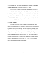
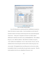
2.6.3 Data Acquisition Cards
There are three data acquisition cards (DAQ cards) attached to the chassis; one for
each pod. There is a USB connection between the laptop and each DAQ card which
allows communication with the LabVIEW software. In this particular setup, LabVIEW is
sending communication signals to the DAQ card, and the card change these
37 communication signals into a physical voltage. The outputs are considered either digital
using TTL logic (0V for false and 5V for true) or are analog where the voltage is
proportional to the command from LabVIEW with a range of 0V to 5V.
For each pod, LabVIEW sends five communication signals to the DAQ cards
which are represented by five channels. Three channels are digital and two are analog.
Two of the digital signals are used to change the direction of each wheel. The last digital
signal is used to simultaneously disable both wheels on a pod. The analog channels are
used to send voltage signals to each wheel which in turn control the velocity of the
wheels. Here 0V is a command of no motion and 5V represents maximum motor speed.
The last function of the DAQ cards is to receive physical signals from the
components on the vehicle. From there, the DAQ cards change those to a communication
signal LabVIEW can interpret.
In this particular set-up, the encoders and the motor controllers send signals to the
DAQ cards. Due to the limited amount of digital channels, all 10 wires from each
encoder were wired to analog channels. It is acceptable to run digital signals on an
analog channel because the software will not be able to detect the difference. A low
signal (0V) or a high signal (5V) can still be interpreted as false or true, respectively, on
an analog channel. The encoders receive their power from the DAQ cards.
The motor controllers send a pulse train signal, generated by the Hall-effect
sensors in the motors, to the DAQ cards. The DAQ cards are able to count the pulses and
use an internal timer to track the velocity of the wheels. Though there are three Halleffect sensors, only two are utilized. This is again due to the limited amount of digital
channels. Unlike the encoders, the Hall-effect sensors need to be wired to digital
38 channels. This is due to the DAQ cards only being able to count the pulse trains on
digital channels. Only the digital channels have counting capability. A minimum of two
pulse trains are needed in order to detect motor direction.
Figure 2-12 shows a data acquisition card and the various pins available for use
on the device. National Instruments makes several Data Acquisition Cards where the
major differences are the number and quality of the channels in the card. The DAQ card
used in this project is model number USB-6215. A detailed description of the wiring
layout and channels as used for this project is described in the wiring section, 2.6.4.
Figure 2-12 Summary of Data Acquisition Card Pin Layout [17]
2.6.4 Wiring
The batteries supply power to motor controllers and ultimately the motors. The
battery leads had to be run through the slip-rings since the batteries are mounted in the
floor pan of the vehicle and the motors and motor controllers are mounted to the pods
which can rotate. The data acquisition cards, encoders, and receiver for the vehicle
controller are all powered by the laptop. The receiver is part of the game pad controller
system. The game pad transmits signals to the software through the receiver. The game
pad will be discussed in detail in Section 2.8
39 The wiring between all the physical hardware mounted to either the chassis or
pods is responsible for all power and signal-level communication. For a given pod this
includes the two motors, the pod encoder, the DAQ card, the battery, and the slip-ring.
The brushless DC motor has eight pins all of which are connected to the controller. They
are conveniently numbered Pins 1-8. A summary of the pin layout is listed in Table 2-2
below [16].
Pin # Pin 1 Pin 2 Pin 3 Pin 4 Pin 5 Pin 6 Pin 7 Pin 8 Connection Hall Sensor 1 Hall Sensor 2 4.5 … 18 VDC Motor Winding 3 Hall Sensor 3 Ground Motor Winding 1 Motor Winding 2 Table 2-2 Motor Pin Summary [16]
The pins of the motor are laid out in two rows of four. The geometry of the pin
layout is more than likely what controlled the pin designation. For instance, Pins 1&5 for
the Hall Sensor 1 and Hall Sensor 3 are not near each other numerically, but they are
physically due to the pin geometry. The pin layout can be seen in Figure 2-13.
40 Figure 2-13 DC Motor Pin Layout [16]
The wiring between the DC motor and the controller is illustrated below in Figure
2-14.
Motor Controller
Motor
Figure 2-14 Wiring diagram between the DC Motor and Controller
The remainder of the wiring is between the pod encoder and the DAQ card and
between the motor controller and the DAQ card. The best way to explain this wiring is
through the simplified wiring diagram shown in Figures 2-15 and 2-16.
41 12
6
8
12 14
28
Figure 2-15 Wiring Set-up between Acquisition Card and Motor Controller
Figure 2-16 Wiring Set-up between Acquisition Card and Encoder
42 The last item is the wiring of the slip-rings. The slip-rings allow a wiring
connection even though the two items being connected may move (rotationally) in
relation to each other. For each pod, the DAQ card as well as the pod encoder is attached
to the chassis of the vehicle. Therefore, the encoder signals do not have to pass through
the slip-ring. The motor controllers (2x) are attached to the top of the pods and,
therefore, need the slip-ring to complete the connection from the pod to the DAQ card.
The power source for the controllers, since it is coming from the chassis, needs to go
through the slip-ring as well. The quantity of each type of channel (analog vs. digital) is
limited by the DAQ card. In general, the total number of channels used on the vehicle
was limited by the slip-rings. A summary of the channels being controlled, the type, and
whether or not it can be shared by the two controllers at the same time is shown in Table
2-3.
Used by both controllers
Power +
Power – (ground)
Analog Ground
Digital Ground
Brake
Disable
Type
Used by separate controllers
5V Control
Direction
Analog
Hall Sensor 1: Motor 1
Digital
Hall Sensor 2: Motor 1
Digital / O Hall Sensor 1: Motor 2
Digital / O Hall Sensor 2: Motor 2
Type
Analog / O
Digital / O
Digital / Ctr.
Digital / Ctr.
Digital / Ctr.
Digital / Ctr.
Table 2-3 Summary of Pin Connections Passing through the Slip-rings
2.7 Masses, Inertias, and Dynamic Characteristics
Most of the mechanical aspects of the device were completed and built by prior
senior design classes, but the masses and inertias of the vehicle components still needed
to be captured for use in the design of the controller and construction of the vehicle
simulation. The mass of the pod as an assembly and the mass of its components
43 (including the suspension components, two wheels and axles, the motors, and the
controllers) all needed to be found and documented. Furthermore, the rotational inertias
of the wheels and the completed pod also needed to be identified. The mass and inertia
of the complete vehicle was taken only after the final layout and composition of the
vehicle was determined. These parameters are important for the vehicle to be modeled
and simulated. The simulation will be discussed in detail in Chapter 5.
The masses of the components were found by placing them on a digital scale.
Finding the rotational inertias of the wheel assembly and completed pod was not as
straightforward as finding the masses of the components. Since the exact make-up
(density and geometry) was not known of the components, the rotational inertias needed
to be found experimentally employing a multi-filar suspension [18] [19].
This encompasses suspending the assembly by two or more wires, inducing an
initial rotational displacement, and letting the assembly oscillate freely. The resulting
period of oscillation and the physical parameters of the experiment can be employed in
Equation 2-1 [18] to estimate the moment inertia of the assembly.
2
J
WR2 L0
t2
2
2
4 ( L0 ( R2 R1 ) )
(Eq. 2-1)
The parameters in Equation 2-1 are shown in Figure 2-17. t is the recorded period of
oscillation, W is the weight of object, and J is the inertia. For the pod assembly, only two
wires were used in the experiment. The chassis inertia was measured using three wires,
though the number of wires used to suspend the component or assembly has no effect on
the measured inertia.
44 Figure 2-17 Test Experiment for Determining the Moment of Inertia of an Object [18]
Table 2-4 includes the experimental inertias and masses of the various
components.
Wheel, Axle & Bearing Assembly
Wheel
Pod Frame
Motor, Mount Plate, 4 Bolts, & 4 Washers
Controller w/Wiring
Entire Pod
Entire Vehicle
Chassis (w/o Pods)
Mass (kg)
1.012
0.570
1.561
0.422
0.136
9.705
55.000
25.885
Table 2-4 Summary of Masses and Inertias
45 Inertia (kg-m2)
N/A
0.00204
N/A
N/A
N/A
0.07238
21.80
18.785
2.8 Human Interface and Control
The PC laptop runs the vehicle software that carries out all of the complex
calculations needed for controlling the vehicle. For this particular application, an IBM
ThinkPad running Windows XP was chosen to run the software used for implementing
the logic that controls the vehicle. The logic for interfacing with and controlling the
vehicle is specifically implemented in LabVIEW. The LabVIEW software is well-suited
to interfacing with physical hardware. Specifically, LabVIEW has a graphical interface
that makes it easy to configure channels that send signals to, and acquire information
from, the vehicle. The LabVIEW software also offers the ability to implement the
algorithms needed for controlling the vehicle.
This particular project is not autonomous and, therefore, requires a human
operator to give commands to the vehicle. Three specific options for wireless control of
the vehicle were considered. The first was a personal digital assistant (PDA). The
advantage of a small computer, like a PDA, is that it can serve multiple functions and can
employ multiple different applications. For example, the PDA can allow the operator to
take notes of what he/she saw while using the vehicle, or he/she can store data sets and
even perform calculations with a program like Excel.
The downside is that it required a peer-to-peer internet or blue tooth connection.
This type of connection is only good within a 30 foot radius. Often times the connections
are intermittent and can be randomly and unexpectedly lost. The connections also take
long durations of time to set up before becoming available for use. Setting up LabVIEW
to interface with the PDA also took large amounts of time and was very difficult to
initiate. This is not a problem if the software was adjusted one time and one time only.
46 However, one particular setup may not work for every operator and hence may require
adjustment. Thus, for the sake of time, the ability to rapidly and accurately change the
control software is an advantage.
Yet another drawback of the PDA is that it did not receive more than one input
from the user. It only accepted one input from a stylus which was a decided disadvantage
since the user would need to input speed and direction simultaneously. The user also has
to take his/her eyes off the vehicle to make sure the stylus is in the correct position on the
PDA screen. This is a severe disadvantage to a vehicle that is supposed to be operated at
a high pace by a soldier that must be aware of his/her environment.
A second option was the use of a cellular phone. A phone like Apple’s iPhone is
able to share the screen and essentially take over the IBM laptop attached to the vehicle.
Screen sharing software could be installed on both the PC and the iPhone and, therefore,
allow total control over the PC. This would be a good approach if there had not been
quality issues related to the screen sharing capabilities. Specifically, long lag time
between inputs to the iPhone and communication to the laptop made it almost impossible
to drive the vehicle without fear of crashing it. The phone and laptop connections also
suffered from the same problems the PDA did. The iPhone required either a wireless
internet connection (Wi-Fi) or bluetooth connection. As stated previously, a Bluetooth
connection is still only good within a 30 foot radius. A Wi-Fi connection is undesired
since the vehicle was intended to be used in an outdoor, possibly remote, setting were
wireless service is often not available.
The third option was a gaming controller as seen on most modern gaming
consoles such as PlayStation, Xbox or other similar consoles. The Xbox 360 controller
47 was chosen since Microsoft makes both the laptop operating system and the Xbox
gaming console. This eliminated any compatibility issues between the controller and the
computer. The controller works as a transmitter and the laptop as the receiver, therefore,
this arrangement offers a more robust wireless connection that works very well up to a
minimum radius of 100 feet. Another upside to the controller is that it allows the user to
control the vehicle while maintaining visual contact 100 percent of the time. The soldiers
of this generation also grew up playing Nintendo, PlayStation, or other similar consoles.
The feel and control of this type of controller is completely natural to this generation of
soldiers.
The raw signals from the game pad controller are also easily read in and can be
easily manipulated within the LabVIEW software. Therefore, setting up and changing
the configuration of the interface with the gamepad controller is quite simple. Lastly,
initializing the connection between the LabVIEW software and the gamepad controller is
fast enough that it is effectively instantaneous. Figure 2-18, below, shows the controller
used for control of the vehicle. The button configuration will be discussed in Chapter 3.
48 Figure 2-18 Xbox 360 Wireless Game Pad [20]
49 3.SoftwareDescription
3.1 LabVIEW
LabVIEW is the software chosen to provide the interface between the hardware
on the vehicle and the commands given by the driver. Within this program, users can
freely set-up algorithms that control or monitor physical devices. These routines are
termed Virtual Instruments or VIs for short. LabVIEW can specifically interface with
these devices through channels of a DAQ card. These channels allow the ability to track
various physical signals within a system or allow control signals to be sent to an array of
actuators. In addition to monitoring signals from traditional sensors, LabVIEW can also
read in real-time, signals from a user such as inputs from a gaming controller.
All of the abilities possessed by LabVIEW come together and allow for the
creation of very specific and customizable environments (programs). Given that a user
has an in-depth knowledge base of LabVIEW, users can set up new programs or edit
existing ones fairly quickly. The reason is that the interface between the user and the
computer screen is very intuitive for setting up programs. The interface utilizes a block
and wire diagram which allows the user to easily see what he/she is doing on the screen.
The blocks can be dragged and dropped from existing libraries and represent some
calculation or process while the wires connect the blocks by simple pointing and clicking
of a mouse and represent signal flow. It is this physical interaction that allows relatively
quick and easy program set-up and editing. It especially provides a simple way to
interact with the physical devices through a DAQ card where much of the underlying
50 hardware interface is handled at a high-level by specifying options from menus built-in to
various existing blocks.
Within LabVIEW, there are two windows used to make VIs. The “front panel” is
a graphical user interface used to either monitor or control something. Physically
intuitive switches, dials, lights, graphs, or readouts can be arranged on this screen again
by dragging and dropping elements from built-in libraries. It is more or less a quick
summary of the physical device the user is trying to control or monitor. Using only this
panel, the user sees the inputs, control or initial settings, and the outputs, such as
pressure, velocity, position, voltage, etc. In the case of this project, the user cannot adjust
anything on the front panel. The inputs, like speed, direction, orientation and emergency
disable, come from the video game controller. The video game controller inputs, wheel
speed, direction of the wheels, pod encoder angles, and emergency stop are monitored on
the front panel.
Keep in mind that the front panel, in this case, was not designed to take inputs
directly from the user since the vehicle will be in motion. Instead, the inputs come from
the video game controller, thus allowing the driver to control the vehicle remotely. The
front panel here was primarily used to monitor the vehicle’s operation and to assist with
the design and debugging of the vehicle during development.
The “back panel” is a separate screen where all hardcoded elements, calculations,
processes, and interactions with the DAQ cards are initiated and take place. The
programmer can open up various channels with the DAQ cards and send the inputs from
the front panel to the actual device. A programmer can either send the control signal
from the front panel straight to the actual device, or the signal from the front panel can be
51 used as an input to some algorithm that calculates commands to be sent to any of the
device’s actuators.
The back panel is also the place to open up a channel on a DAQ card and pull in
signals from the device. Similar to the signals sent to the device, the received signals can
also go through some processing before being displayed on the front panel or sent to
another portion of the back panel. For instance, data from the Hall-effect sensors on the
motors is recorded as pulses representing changes in angular position, but is not of much
use to the driver or to someone trying to model the vehicle. Therefore, an approximate
derivative of the position is calculated to estimate wheel speed before being written to a
file or displayed on the front panel. This information is much more valuable than the raw
position data initially read from the sensor.
3.2 Overall Vehicle VI
The front panel for the overall vehicle control program, shown in Figure 3-1,
allows the user to monitor various aspects of the vehicle.
52 +/-100%
ω (rad/s)
Figure 3-1 Front Panel Screen Shot of the Overall Vehicle VI
Five volts is the saturation limit on the brushless DC motors. Therefore, the voltage sent
to the motors is held to within +/- 5.0 volts by the DAQ card. The range of possible
voltage inputs (from Vx and Vy), from the driver, can be characterized by an imaginary
circle centered at the origin of a coordinate system. This coordinate system, as
mentioned in Chapter 2, has its origin located at the center of gravity on the vehicle and
remains fixed to the vehicle. This “voltage circle” would have a radius of five units
representing the five volts. The driver can send the vehicle any voltage combination as
long as it is within this circle which is shown in Figure 3-2.
53 Figure 3-2 Voltage Circle
This coordinate system can be seen on the front panel of the vehicle, shown in Figure 31. In LabVIEW, the imaginary circle is represented by two sliders; one for the y-axis
(Vertical, Vy) and one for the x-axis (Horizontal, Vx). The last slider (Vertical, Velocity)
represents the velocity control as given from the gamepad and can range between +/100% (0-100% forward or 0-100% reverse).
Both the Velocity scaling and the x- and y- coordinates of the velocity need to be
commanded in order for the vehicle to move. This method for vehicle control was set-up
to improve control over the vehicle. It was assumed that the user will automatically
move the coordinate control (left analog stick on the gamepad) to its extreme when
operating the vehicle. This would represent a full five volts to the motors in any given
direction. The right analog stick on the gamepad is used to control a percentage of the
voltage. Since the motors are operated in closed-loop speed control mode, the right
54 analog stick also represents a percentage of the velocity and that is why it is labeled as
such. Only a forward and reverse movement is registered on the right analog stick on the
gamepad. Again, the analog sticks on the gamepad were set-up in this fashion to increase
control over the vehicle. This was thought to be amongst the most intuitive methods for
controlling the vehicle with the gamepad.
The dial indicator marked Rotation displays the angular speed (rad/s) commanded
of the chassis. This is also a command given by the gamepad. The sliders and dial
indicator are used as a display only. These are used only to display what the gamepad is
sending to the laptop and, therefore, the vehicle.
The two red lights on the right hand side of the front panel indicate the vehicle
status. The vehicle can be run with or without the feedforward portion of the control
system turned on as indicated by the red light towards the top of the front panel. Running
the vehicle without the feedforward control system only allows the alignment of the pods.
It does not allow any physical movement of the chassis. The feedforward and feedback
portions of the control system were split up again to allow more precise control of the
vehicle. In particularly tight situations, it may become advantageous to orient the pods
prior to translating or rotating the chassis. This will also aid in ensuring the safety of the
vehicle and its surroundings.
The bottom red light on the front panel shows whether or not the emergency stop
(E_stop) function is activated. If it is activated, the motor controllers will cease to
receive inputs from the gamepad and will coast to a stop due to rolling and air resistance.
The rest of the indicators are output values based upon the physical status of the
vehicle. Reverse light indicators, on the left of the front panel, are just a quick way of
55 telling if the wheels on each pod are running in reverse. Odd numbered wheels are the
left wheels on the pods while the even numbered are right wheels. Wheels one and two
are on pod one. Pod two houses wheels three and four and wheels five and six are
attached to pod three. The Pod Angle indicators show the actual pod angle in relation to
the chassis in radians. The numbered wheels, pods, and pod angle calculation method is
shown in Figure 3-3.
Figure 3-3 Pod and Wheel Numbering System
In Figure 3-3, the pods are currently aligned at π/2 radians in relation to the chassis. This
is an example of how the pod angles are calculated both in LabVIEW and in the
simulation.
The delta T box, shown in Figure 3-1, towards the left hand side of the front
panel, shows approximately how much time has passed since the last iteration of the
algorithm loop implemented in the back panel.
56 The P, I, and D gains and the Max Speed voltage controls on the upper left hand
portion of the front panel allow the operator to quickly change the gains on the control
system and the maximum allowable voltage that the motors are allowed to receive. Each
voltage control represents one pod and, therefore, two wheels. Although the maximum
allowable voltage is separate for each pod, the voltage limit should be set to the same
value for all three pods. These controls are only there temporarily for design and
debugging purposes. The final layout for the vehicle’s front panel will not include these
items. The last point to keep in mind is that all of the items displayed on the front panel
are there for monitoring purposes or initial set up. They are not essential for the control
of the vehicle and most likely will not be used by the driver once he/she starts to drive the
vehicle.
On the back panel, the overall vehicle VI starts with receiving inputs from the
gamepad. Those inputs are then sent to the feedforward (inverse kinematics) and to a
sub-VI that calculates the desired pod angles. Calculated results from the Feedforward
Sub-VI and the Desired Pod Angle Sub-VI are sent to the Closed Loop Control Sub-VI.
The actual pod angles are also sent to the Closed Loop Control Sub-VI. The Closed
Loop Control Sub-VI makes adjustments to the wheel voltage signal and, therefore,
corrects for any error that may be present in the system (vehicle). The wheel voltage
signals then flow from the Closed Loop Control Sub-VI to the Pod Voltage Control SubVI. A screen shot of the entire back panel is too large to be placed within this document
and, therefore, is replaced with a block diagram that summarizes the Overall Vehicle VI
back panel. This is shown in Figure 3-4.
57 Figure 3-4 Overall Vehicle VI Back Panel Summary Block Diagram
The VIs within LabVIEW are an iterative process which means that the program
runs one series of calculations (gamepad inverse kinematics/desired pod angle
closed loop control motors) and then terminates upon completion. This is considered
to be one iteration of the loop. The vehicle, however, is dynamic and thus may require
several iterations per driver command. To combat this issue, LabVIEW has built-in loop
features.
In order to keep the VI running, a timed loop structure was placed around the subVIs and the gamepad controller inputs. The timed loop will continue to run until the user
stops the Overall Vehicle VI. The loop used on the vehicle continues to run an iteration
once every 1/5th (0.2) of a second, within precision limits. LabVIEW will continue to do
this until the user stops the program from the laptop. It is desired that the time between
each iteration of the loop be as low as possible. However, the complex calculations
58 within the Overall Vehicle VI will not allow the use of cycle times less than
approximately 0.2 seconds.
The signals read from the gamepad come in as raw signals and need to be
conditioned before they are usable by the vehicle control algorithm. The three most
important signals are the x-component and y-component of the vehicle’s velocity and
desired angular velocity, ω. These signals are used to calculate desired pod angles, in
relation to the chassis, which in turn are used as inputs to the vehicle control system. All
of these calculations aid in better overall control for the driver. More detail on the
gamepad controls will be given in Section 3.3.
Signals from the video game controller are fed directly to the feedforward control
system (Inverse Kinematic Model Sub-VI) and to the Desired Pod Angle Sub-VI. The
feedforward control system helps to send the proper motor voltage to each of the six
wheels. The voltage each wheel receives, prior to the correction offered by the PID
controller, is dependent on the current angle of the pod, in relation to the chassis, and the
control signals given from the gamepad. The Desired Pod Angle Sub-VI calculates what
the pod angles should be for a given command from the gamepad. This gives the closedloop control system its setpoint. More information on the Desired Pod Angle Sub-VI and
Inverse Kinematic Model Sub-VI is given in Sections 3.5 and 3.6, respectively.
The Encoder Sub-VI provides the vehicle with actual pod angle measurements.
The Encoder Sub-VI will be discussed in detail in Section 3.4. These measurements, one
angle from each of the three pods, in conjunction with the desired pod angle
measurements help calculate the error for the closed-loop control. Inside the PID Gains
Sub-VI, the actual pod angle is subtracted from the desired pod angle or setpoint, for each
59 particular pod, which becomes the error. The error undergoes additional conditioning
before being fed into the PID gains. Details on how the error is conditioned are discussed
in Section 3.7. Once the error has been adjusted with the control gains, it is sent to the
Control System Sub-VI.
The Control System Sub-VI takes inputs from the PID Gains Sub-VI and the
feedforward control signals to generate each individual wheel voltage for that particular
loop iteration. The feedforward control should provide wheel voltages that are close to
what the vehicle needs. The closed-loop control system in essence corrects the
feedforward command to account for errors and disturbances. The control effort
calculated by the closed-loop control system is divided by two. One half of the control
effort is subtracted from the left wheel and the other half is added to the right wheel on
the pod. This will induce a net torque on the pod which helps to change its direction and
ultimately reach the setpoint. The Control System Sub-VI and the overall control
strategy will be discussed in Section 3.7
Six voltage commands representing desired speed, one for each wheel, are output
from the Control System Sub-VI and routed upwards on the back panel. They are
received at the Pod Voltage Control Sub-VI. There are three Pod Voltage Control SubVIs representing each of the pods. Two voltage signals are fed into each of these VIs.
The voltage signals are specific to its intended wheel so it is important that each signal is
connected to its correct input. The Pod Voltage Control Sub-VI simply opens up the
channels to the DAQ cards so that the voltage signals can be sent to the motor controllers
and eventually the motors. Section 3.8 contains detailed information on the Pod Voltage
Control Sub-VI.
60 3.3 Gamepad Controls
Figure 3-5 shows the Gamepad Sub-VI. There is no front panel to this VI so only
the back panel is shown. The Gamepad Sub-VI could have been embedded as its own
Sub-VI, but was left as a part of the Overall Vehicle VI to allow users/drivers to quickly
set-up and alter the gamepad controls. Once the controls are finalized, this VI can be
embedded as a sub-VI in the Overall Vehicle VI.
Figure 3-5 Gamepad VI Back Panel
The Init Joy Icon on the left-hand side of Figure 3-5 sets up the lines of
communication between the gamepad controller and LabVIEW. This sub-VI resides just
outside of the loop since it only needs to be run once per session or once each time the
vehicle is used. The sub-VI to its immediate right opens up the channels on the gamepad.
Each channel represents a specific button, so care was taken to identify what channel
controlled what button. The buttons chosen to control various aspects of the vehicle can
61 be chosen based upon user preference and can be altered at any time. The current
gamepad setup, the actions of each of the buttons, joysticks, and bumpers perform, is
shown in Figures 3-6 and 3-7.
“Y”-Direction
+
+
+ Speed
“X”-Direction
Disable
Feedforward
Control
Toggle
ON/OFF
- Speed
Figure 3-6 Gamepad Button Summary (Front) [20]
62 Clockwise
Counter-clockwise
Figure 3-7 Gamepad Button Summary (Back) [21]
Table 3-1 describes the function of each button based on Figures 3-6 and 3-7.
Control Name
Type
Range
Activation
y-component Velocity
x-component Velocity
Speed Multiplier
Chassis Rotation
Disable
Feedforward Control
Analog
Analog
Analog
Analog
Digital
Digital
+/- 5V
+/- 5V
+/- 100 %
+/- 0.5 rad/s
On / Off
On / Off
Left Joystick (Up/Down)
Left Joystick (Right/Left)
Right Joystick (Up/Down)
Triggers
X-button (hold to disable)
A-button (Tap, Toggle )
Table 3-1 Gamepad Button Summary
As described in Section 3.2 and in Table 3-1, the left analog stick on the gamepad
has a maximum value of five volts in any direction. This again can be represented by an
imaginary circle with a radius of five which is centered at the origin of a coordinate
system local to the CG of the chassis. The driver can request a velocity vector which is
broken into x- and y-components of velocity depending on the position of the left analog
stick.
63 On the back of the controller, as shown in Figure 3-7, there are triggers. Both
triggers are part of one axis. The left is for negative values while the right trigger stays
positive. Holding down both triggers at the same time cancel one another out and the
value goes to zero. This value/axis is reserved for the angular velocity control, ω, of the
vehicle. A full deflection of one of the triggers will request the vehicle to rotate about its
Z-axis with an angular speed of +/- 0.5 rad/s depending on which trigger is pulled.
The signals are read in as integers with a range dependent on the number of bits of
the channel being used, in this case 16 bits: one bit for the sign of the raw signal and 15
bits for the controller signal. In order to modify the axis values to something usable for
the vehicle, each raw signal was divided by the maximum value given by the possible
value (215, 32768). This normalizes each signal to a range from -1 to +1. From there,
each analog was multiplied by a scale usable for the vehicle. In the case of the x- and ydirections, the signals were multiplied by five to give a range of +/- 5. The speed control
signal was not scaled since a range of +/- 1 was desired. This represents +/- 100% of the
speed commanded to the vehicle. A negative percentage means the vehicle is instructed
to go in reverse. The axis for rotation was multiplied by 0.5. This does not have as wide
of a range as the other signals due to vehicle characteristics found during testing. There
was no need to require the vehicle to make sharper turns.
These controls are set up based on the preferences of one or two users. Other
users may find it necessary to adjust the range of each input to suit their driving style or
needs. The most probable adjustment is the rotation command, especially when various
terrains place different demands on how the vehicle should turn.
64 The X-button on the gamepad controls the disable function on the vehicle. By
pressing and HOLDING this button, the vehicle will become disabled and will coast to a
stop regardless of any other commands given by the gamepad. The vehicle will continue
to be non-responsive to other gamepad inputs as long as the X-button is HELD.
The A-button controls the feedforward control portion of the control system. This
button was setup to act as a toggle. TAPPING the button once will either turn the
feedforward control on or off depending on the initial state of the feedforward control.
For example, if the feedforward control was on and the A-button was tapped, the
feedforward control would then be turned off and vice versa. It is also the case that none
of these button or axis configurations are permanent. The controls can be configured to
suit the preferences of any user.
3.4 Encoder Sub-VI
The pod encoders are able to track the angle of the pod with the help of a matrix
of numbers, combinations of zeros and ones. This matrix is located within the Encoder
Sub-VI. Figure 3-8, shows this matrix. There are three encoders so there are three subVIs. Each sub-VI and its calculations are performed independently for each pod. The
encoders used on the vehicle are optical and output a 10-bit binary number which
correspond to the angular position of the shaft inside the encoder casing. Since the
encoders are 10-bit or has 10 wires that carry a signal, the total number of position
combinations is 210, or 1024 combinations. The number of combinations is the number
of sectors the encoder can be divided into. A greater number of sectors reflect a more
precise angle measurement. Therefore, the angular position can be tracked to within
65 360/1024 or 0.352 degrees per sector. In comparison, an encoder that only had three
wires would only have 23 (8) sectors. This brings the angle measurement to within 360/8
or 45 degrees.
Figure 3-8 Encoder VI Back Panel (Matrix Comparison)
Array 2 is a 1x10 matrix that is made up of ones or zeros, in other words, it is the
10-bit binary number. The ones and zeros correspond to a high voltage (1) or a low
voltage (0) signal passed through the connections made between the pod encoder and the
data acquisition card. Each different binary number corresponds to a different position of
the shaft in the encoder. As the encoder and the shaft to which it is attached changes
position, the voltages from each of the channels are passed through the wires connected
to the data acquisition card. That data is eventually placed in Array 2 where it is
compared to a hardcoded matrix that maps each binary number to a different angular
position.
The hardcoded 1024x10 matrix is included in the back panel of the VI. Only the
first three rows are shown in Figure 3-8. This matrix includes all possible combinations
66 where a “1” is represented as true and a “0” is represented as false. By comparing the
actual data, Array 2, to the hardcoded matrix, the angle can be tracked to within
approximately 0.352 degrees. LabVIEW runs a while loop, which compares the array
data produced by the encoder to the hardcoded matrix, until there is a match. The
number loop iterations it took LabVIEW to find the match corresponds to that particular
sector in the encoder. For example, say it took LabVIEW 56 loop iterations to find a
match to the data in Array 2. That would correspond to the 56th sector in the encoder.
This places the encoder shaft between 19.688° and 20.039°.
The green LED's on the front panel, shown in Figure 3-9 are for observational
purposes where each LED corresponds to each digit of the binary number read from the
encoder and are there mostly to make sure the VI is running correctly.
As each wire receives a voltage input, a high input (1) will cause the LED to light
up and a low input (0) will cause the LED to be off. The x*y value is the encoder angle
and the readout labeled Numeric is the number of loop iterations or sector the encoder is
currently positioned. The encoder angle is eventually routed to the front panel of the
Overall Vehicle VI.
67 Figure 3-9 Encoder VI (Front Panel)
3.5 Desired Pod Angle Sub-VI
The Desired Pod Angle Sub-VI calculates a desired pod angle, θi , based on the
user inputs from the gamepad: Vx, Vy, and ω. There are three outputs from the Desired
Pod Angle Sub-VI. All three are pod angles which become the setpoint (in relation to the
chassis) for each of the pods within the closed loop control system. These angles are
compared to their respective pod’s actual angle thereby producing an error signal to the
closed loop control system. The front panel for this sub-VI does not serve any purpose to
the Overall Vehicle VI other than for diagnostic reasons.
Again, the Desired Pod Angle Sub-VI produces a requested angle or desired angle
relative to the chassis. This angle is also based on the chassis’s local coordinate system
shown in Figure 3-2. The basis for the desired pod angles calculation is a kinematic
analysis which is summarized in Equation 3-1 [1].
68 The velocities of the pods can be broken down into their x- and y-components
through matrix operations using the vehicle’s physical parameters and three inputs from
the driver. In Equation 3-1, the driver inputs a desired velocity in terms of the chassis’s
components including translational velocity in either the x- or y-direction and in the
rotational direction by specifying a yaw rate, ω. The outputs are the velocity of each pod
broken down into their x- and y-components. For example, V1,x is the x-component of
the velocity of Pod 1. This is why the output of Equation 3-1 is a 6x1 matrix.
The N-matrix is a 6x3 matrix which contains a B term and φ terms. The B term is
the distance, in meters, from the geometrical center of the chassis to the center of a pod
(same for all pods). For this vehicle, B is 0.58928 meters. The φi terms represent the
angular position from the x-axis (0 radians) of the attachment point of each pod. These
angles are again based on the chassis’s local coordinate system shown in Figure 3-2 and
are constant since a body-fixed coordinate system is used.
V1, x 1
V
1, y 0
V2, x 1
V2, y 0
V3, x 1
V3, y 0
0 B sin 1
1 B cos 1
Vx
Vx
0 B sin 2
V y N V y
1 B cos 2
0 B sin 3
1 B cos 3
(Eq. 3-1)
The x-axis is designated as zero (0) or 2π radians and the angle increases as a pod
or encoder is rotated counter-clockwise. This forces the φi value for each pod. As shown
in Figure 3-3, Pod 1 has an angle of 5π/6 radians or 150˚. Pod 2 is at π/6 radians or 30˚,
and Pod 3 is at 2π/3 radians or 270˚. Figures 3-10 and 3-11, help explain the origin of the
values in Equation 3-1.
69 θ
Figure 3-10 Breakdown of Various Kinematic Inputs on the Vehicle
Figure 3-11 The Orientation of Pod Joints in Relation to the Chassis As shown in Equation 3-1, the resulting 6x1 matrix of velocities, broken down by
their x- and y-component for each pod can be used to calculate the desired pod angle.
Assuming that the pods are oriented such that the wheels are pointed in the direction of
70 the desired velocity, the desired pod angle θi is calculated by taking the inverse Tangent
of the quotient of the y- and x-component velocities; θi=Tan-1(Vi,y/Vi,x) where i is the
index of the particular pod. LabVIEW contains an atan2 function block that keeps track
of the quadrant the angle θi should be in so as to output the true angle. The atan2
function block differs from a standard Tan-1 function because it has a range of –π to +π.
The standard Tan-1 only has a range between –π/2 and +π/2. The back panel of the
Desired Pod Angle Sub-VI helps to illustrate the construction of the matrices shown in
Equation 3-1 as shown in Figures 3-12 and 3-13.
1
N-Matrix
2
Vx
User Inputs
Vy
ω
Figure 3-12 Desired Pod Angle VI Back Panel (Construction of the N-Matrix and User Inputs)
71 1
N-Matrix
Pod Angles
2
Figure 3-13 Desired Pod Angle VI Back Panel (N-Matrix and Pod Angle Output)
After the atan2 function block, each of the pod angle signals undergo a shift to
ensure that the range of the calculated angle is always between 0 and 2π radians.
Otherwise, the default angle ranges between –π and +π.
3.6 Inverse Kinematics Sub-VI
Similar to Equation 3-1 in Section 3.5, a kinematic relationship was derived based
on the geometry of the vehicle which relates the velocity of a pod to the velocity of its
wheels as described in Equation 3-2. Specifically, Equation 3-2 shows the relationship
between the joint velocity Vi (where the pod connects to the chassis) and the velocities of
the left and right wheels on the pod, Vi,l and Vi,r.
Vi , x 1 / 2 cos( i ) S / D sin( i ) 1 / 2 cos( i ) S / D sin( i ) Vi , r
Vi , r
V
V J i V
i ,l
i , y 1 / 2 sin( i ) S / D cos( i ) 1 / 2 sin( i ) S / D cos( i ) i ,l
72 (Eq. 3-2) [1]
In Equation 3-2, Vi,x and Vi,y, are the velocity components of the pod joint where
the subscript i is the ith pod on the vehicle. S is the caster distance or the planar distance
from the center of the wheel axle to the center of the joint connecting the pod to the
chassis. D is the distance between the centers of the right and left wheel on each pod.
The S/D ratio for this vehicle is 1.2 with S equal to 0.75 in and D equal to 6.25 in. Units
do not matter in this case since the number is a ratio of two distances. The S and D
dimension are shown in Figure 3-14. The αi value is the encoder angle for each pod and
would change based upon the current status of the vehicle. Note that the matrix
containing the S, D and αi values is called the J-matrix.
Conventional wheels
Vehicle Chassis
Hinge joint
Split D
Offset S
Figure 3-14 Pod Geometry Description [1]
The 2x2 J-matrix from each pod can be combined to create a 6x6 matrix which
describes the entire vehicle. Using the 6x6 J-matrix from Equation 3-2 can help calculate
the left and right wheel velocities for each of the wheels on the vehicle. Equation 3-3
shown below inverts the J-matrix and multiplies it by the N-matrix and the control input
vector from Equation 3-1. The J notation is used in Equation 3-3 instead of rewriting all
of the terms and to help clarify that there are three pods.
73 V1, r
V
1,l J
V2, r 1
0
V2,l 0
V3, r
V3,l
0
J 2
0
0
0
J 3
1
Vx
N V y
(Eq. 3-3)
The back panel from the Inverse Kinematic Sub-VI shows the block-by-block
construction and multiplication of these matrices. Most of the architecture is shared from
the Desired Pod Angle Sub-VI with additional multiplication as shown in Equation 3-3.
Figure 3-15 shows the construction of the J-matrix, N-matrix, and the inverted J-matrix.
(J-Matrix)-1
J-Matrix
N-Matrix
User Inputs
Figure 3-15 Feedforward Control Back Panel (Construction of Equation 3-1)
Figure 3-15 also shows the multiplication of the user inputs and the inverted Jmatrix. Figure 3-16 shows the additional steps taken to make sure that the output values
for each wheel are normalized to +/- 5 volts thus preventing the saturation of the motors.
The output is a 6x1 matrix of normalized wheel voltages. The direction is taken care of
74 with the sign on the voltage. Negative values signal a wheel running in reverse and vice
versa.
Vector of Wheel Voltages
Voltage Normalization
Figure 3-16 Feedforward Control Back Panel (Wheel Voltage Calculation and Normalization)
If this vehicle were to run in open-loop control, the pod angles (αi) fed into this VI
would be the actual pod angles as read by the encoders. This approach would produce
the desired wheel speeds at any given instant if the models were correct and there was no
slip at the wheels. Since the vehicle will employ feedback, the angles (αi) employed in
this VI to calculate the matrix J have been changed to the desired pod angles (θi). This is
to trick the inverse kinematics into thinking that the pods are already aligned where they
should be. This will make the feedforward controller output the same voltage between
the left and right wheels when it is desired to travel in a straight line. It will also output
the appropriate voltage in steady-state between the right and left wheel when turning if
there is no error in the system. All of this is done to help the performance of the closedloop control system. The concern is that the feedback portion of the controller will fight
against the feedforward portion of the controller if both controllers are sent the actual pod
75 angles (αi). By employing only the desired pod angles in the feedforward controller, only
the closed-loop controller eliminates the error in the system. This approach helps to
decouple the two controllers and was found to make the vehicle easier to tune and more
predictable while being driven.
3.7 Closed-loop Control System Sub-VI
The purpose of the control system is to close the loop and provide feedback at the
pod level in order to assist the driver with achieving a desired heading for the vehicle.
This was found to be necessary due to the significant wheel scrubbing and slip that made
open-loop control unusable at all but the slowest speeds. A pod-level approach to control
was decided on due to the speed advantage the pod control had over chassis control. This
was also decided since the driver could theoretically correct for disturbances at the
chassis level, but not at the pod level. The control strategy and reasons why the particular
controller type was chosen will be discussed in detail in Chapter 5.
A simple proportional-integral-derivative (PID) controller was used on this
vehicle and is shown in the PID Gain Sub-VI. An Integral and derivative function were
both available in LabVIEW, but the integral function did not have an option for antiwindup or error reset. For this project, emphasis is placed on speed. Having an
integrator with no error reset might lead to excessive overshoot and, therefore, take more
time for the pod to reach steady state. Scrubbing and slip in the wheels as well as stiction
in the slip-rings all cause the pods to take longer to reach a commanded, steady-state
angle in relation to the chassis. Therefore, a new integral function was required for the
vehicle.
76 The derivative function within LabVIEW worked well, so it was utilized in the
PID Gain Sub-VI. Figure 3-17, shows a portion of the back panel for the PID Gain SubVI which highlights the integral and derivative functions.
Proportion
Integral
Derivative
Figure 3-17 PID Gain VI Back Panel
As shown in Figure 3-17, the integral function is a simple four line conditional
statement that checks for the current state of the error and then proceeds in adding the
new error. If the error changes sign (negative to positive or positive to negative) then the
error is set to zero (0). The integration of the error is approximated using the trapezoidal
rule and so the Δt, or time between each loop iteration within LabVIEW, is used as the dt
value within the summation. In Figure 3-17, the err1 represents old error or the initial
error, while err2 is the new error or the summation of the error. Depending on the
condition of err1, the integral function will either continue to add the error or set it to
zero (0) for the next loop iteration.
77 The error is calculated by subtracting the actual pod angle of each pod from the
desired pod angle setpoint. This subtraction is shown in PID Gain Sub-VI Back Panel in
Figure 3-18.
PID Control Gains
Control Effort and
Direction Sub-VIs
Error Calculation
Figure 3-18 PID Gain VI Back Panel (Error Calculation)
The error is in units of degrees and would normally be available for direct use in
the control system. However, each pod can revolve 360 degrees and end up back in the
same location as it started. This creates a problem when the pods read 360 degrees since
this could also read 0 degrees. This is especially of concern when the setpoint is near 0
degrees.
There is also a problem with symmetry when using the direct subtraction. Once
the error reaches +/- 180 degrees away from the setpoint, the vehicle would have trouble
knowing whether to go clockwise or counter-clockwise to correct the error. Preliminary
testing showed that the vehicle often would take the longest path back to the setpoint.
78 The Control Effort and Direction Sub-VI within the PID Gain Sub-VI takes care
of these problems and still keeps the error linear with a few piecewise functions. One
piecewise function controls the magnitude with a maximum control effort requested at +/180 degrees of error and no control effort requested at 0 or 360 degrees. A second piece
wise function accounts for the direction such that the pods take the shortest path back to
the setpoint. At 180 degrees of error, where the pod could go either direction, the
piecewise function dictates that the pods turn clockwise by default. This could have
easily been set to rotate counter-clockwise. In this scenario, directional values that are
positive make the pods go clockwise. Values that are negative make the pods rotate
counter-clockwise. Figure 3-19 shows the Control Effort and Direction Sub-VI within
the PID Gain Sub-VI.
Figure 3-19 Control Effort and Direction Sub-VI within the PID Gain Sub-VI
79 In Figure 3-19, the error comes is the input to the Control Effort and Direction
Sub-VI which gets processed through both of the piecewise functions and then is output
on the right side of the VI. The CE value represents the modified error or corrected error
and ranges between zero (0) and one (1). The D value represents the direction and is
either equal to zero (0), negative one (-1), or positive one (+1). These two values are then
multiplied in the PID Gains Sub-VI where the result represents both a direction and
magnitude of error. This is the error that is then fed into the proportional, integral, and
derivative terms. Figures 3-20 and 3-21 show the piecewise functions graphically.
Corrected Control Effort vs. Pod Error
1.2
1
Control Effort
0.8
0.6
0.4
0.2
0
-400
-300
-200
-100
0
Pod Error
100
200
300
Figure 3-20 Control Effort Calculation as a Function of Calculated Pod Error
80 400
Control Direction vs Pod Error
1.5
Control Direction (+/- 1)
1
0.5
0
-400
-300
-200
-100
0
100
200
300
400
-0.5
-1
-1.5
Pod Error
Figure 3-21 Direction Calculation as a Function of Calculated Pod Error
For each pod, the corrected error is multiplied by each of the gains. The three
terms are added to make an overall control effort for each pod. This overall control effort
is then sent through the PID Gain Sub-VI and out into the Overall Vehicle VI. The three
control effort signals, one for each pod, are then routed to the Control System Sub-VI. In
this VI, the control effort signals for each of the pods and the voltage signals from the
feedforward controller are added together to create a final set of voltages for each of the
six wheels. Figure 3-22 shows the back panel for the Control System Sub-VI.
81 Corrected Control Effort
Normalization VI
Feedforward Wheel Voltages
Figure 3-22 Control System VI Back Panel
In the Control System VI, the corrected control effort for each pod is divided by
two. One half of the control effort is subtracted from the left wheel and the other half is
added to the right wheel. This induces a net torque on the pod as long as there is a
correcting signal coming from the PID Gains Sub-VI. Subtracting the effort from the left
and adding to the right wheels ensure that the pods rotate in the correct direction as
instructed from the PID Gains Sub-VI.
Simply adding the control effort to the feedforward voltages creates a potential for
a total wheel voltage to be greater than 5 volts. To combat this, another sub-VI called the
5 Volt Normalization Sub-VI was added to bring the range to within +/- 5 Volts. Most of
the coding within this VI was borrowed from the Inverse Kinematics Sub-VI since it
included a 5 Volt normalization procedure. The back panel for the 5 Volt Normalization
Sub-VI is shown in Figure 3-23.
82 5V Normalization
Figure 3-23 5-Volt Normalization VI Back Panel
The left side of the VI is the addition of the feedforward control voltages with the
corrected control effort values. The VI then checks the 6x1 matrix of values to see if the
absolute value of any of the voltages is greater than five. If one of the voltages exceeds
+/- 5, the matrix is divided by the absolute value of the maximum value and then
multiplied by five. Performing the normalization in this manner keeps the size of the
commands to the individual wheels the same relative to one another. This has the effect
of maintaining the overall desired heading of the vehicle. If none of the voltages exceed
+/- 5, the matrix is passed through without scaling. The output, right side of the VI, is a
6x1 matrix of usable voltages. Directly to the right of the 6x1 matrix are LabVIEW
blocks that extract individual values from the matrix depending on the index number
given to the block. Eventually all six wheel voltages are extracted from the matrix so that
the individual wheel voltages can be routed to the rest of the Overall Vehicle VI as
needed.
83 3.8 Pod Voltage Control Sub-VI
The final wheel voltages calculated in Section 3.7 are routed from the Control
System Sub-VI within the Overall Vehicle VI to the three Pod Voltage Control Sub-VIs.
There is one Pod Voltage Control Sub-VI for each of the pods. Of the six wheel voltages
found in the Control System Sub-VI, there are three left and three right wheel voltages.
One left and one right wheel voltage, corresponding to their respective pod number, is
routed to each Pod Voltage Control Sub-VI. The result is that “Pod 1 Voltage Control
Sub-VI” represents pod one. The final left wheel voltage one and the final right wheel
voltage one, CVL1 and CVR1, are both routed to Pod 1Voltage Control Sub-VI.
The Pod Voltage Control Sub-VI is very simple. In this VI, there are five
channels opened up on the DAQ card. Three are digital signals and the last two are
analog. The analog signals are the voltage signals that command the individual wheel
speeds. There is one analog signal for the left wheel and one for the right wheel. In this
VI, the sign (+ or -) is extracted from the analog signal, converted to a digital signal, and
used to maintain the wheel’s direction. Positive values mean that it is desired that the
wheel roll forward and negative values mean that the wheel is to roll backward. The left
side of Figure 3-24 shows where the wheel voltages come in and where the DAQ
assistant block opens up the analog channels on the DAQ card.
84 DAQ Assistant (Analog)
Figure 3-24 Pod Voltage Control Sub-VI Back Panel (Analog Signals)
The extracted sign from the wheel voltage represents a digital signal, so there is
one signal for each of the two motors. The sign from the wheel voltages are converted
into a Boolean operator where a negative value will cause the operator to be true and will,
therefore, reverse the motor. A true value coming from the VI produces a physical
command of 5 Volts to the direction channel of the motor controller while a false value
produces a command of 0 Volts.
The last digital signal is for the wheel disable. Only one signal is needed for this
since we will always disable both wheels on a given pod together. Similar to the wheel
direction signals, the disable is a Boolean operator. When the disable button on the
gamepad is depressed, a high value (1) will be sent to the Boolean operator and converted
to true or false. A value of (1) represents a true value and so the DAQ card sends a 5 volt
signal to the motor controllers to disable the brushless DC motors.
Similar to the analog DAQ assistant, the digital DAQ assistant opens up three
digital output channels, instead of analog outputs, on the DAQ card. This will allow the
high and low signals to be sent to the motor controllers. As shown in Figure 3-24, all
three of the digital signals are routed through this DAQ assistant. The Pod Voltage
85 Control Sub-VI corresponding to the other two pods are analogous to the one shown in
Figure 3-24.
86 4.VehicleParameterization
4.1 Modeling Preparation
In preparation for modeling the vehicle in simulation in Chapter 5, it is necessary
to characterize the vehicle using measured data. The development of a tire model is the
most important application of this data, but other parameters such as air resistance, slipring friction, and motor characteristics are also important aspects of the vehicle model
that must be identified. The remainder of Chapter 4 will break down these
parameterizations. Furthermore, the test procedures used to gather this data will be
explained in detail as Chapter 4 progresses.
4.2 Tire Model
A great deal of time could have been spent on the tire model alone. More time
spent characterizing the model yields improved accuracy of the simulation in terms of the
predicted longitudinal and lateral acceleration of the vehicle during different types of
maneuvers. There are many things that could be taken into consideration when
characterizing the tire equipped on the vehicle. Normal load, temperature, air pressure,
surface roughness, surface material, and suspension set-up all play a role in how the tire
performs on the vehicle.
In the interest of time, just three parameters describing the tires equipped on the
vehicle were studied. Furthermore, these parameters were studied using a relatively tight
range of conditions. Currently, the vehicle is run indoors on one surface. So for
modeling purposes, the tire was characterized using only one friction surface; the shop
87 floor in the engineering building highbay. Since the vehicle was always run indoors, the
temperature remained fairly consistent from test to test. The vehicle was not driven to the
limits of traction enough to force heat or air pressure build-up in the tire. Tire pressure
was kept at 20psi on all six wheels and consistent suspension geometry was maintained
on the vehicle. Given these initial conditions and assumptions, the vehicle was tested for
longitudinal tractive force, lateral force, and rolling resistance [22].
4.2.1 Rolling Resistance
The first piece of tire information needed to describe the tire is the rolling
resistance. To acquire this information the vehicle was accelerated and then allowed to
coast to a stop. For this test, only the deceleration portion of the data was considered.
Once again, vehicle velocity was estimated from the DC motor’s Hall-effect sensors
assuming no-slip since the wheels were not being driven during the coast-down.
The derivative of the velocity curve gave the deceleration profile. This profile
was multiplied by the mass of the vehicle to give the total resistance force during the
deceleration period, including air resistance. As the velocity approaches 0 m/s, however,
the force drastically falls to zero. The force value recorded just prior to the force falling
to zero is representative of the rolling resistance. There is a great deal of noise generated
by the Hall-effects sensors which is shown in Figure 4-1. Nonetheless, straight lines
were fit to the data. Figure 4-1 is just one of the data sets acquired from the vehicle.
88 80.0
70.0
y = 5.3124x + 14.844
R² = 0.7174
60.0
Force (N)
50.0
40.0
30.0
20.0
10.0
0.0
‐1.0
0.0
1.0
2.0
3.0
4.0
5.0
6.0
7.0
8.0
9.0
10.0
Velocity (m/s)
Figure 4-1 Coast-down Test Results for Determining Rolling Resistance
The y-intercept of the data set, shown in Figure 4-1, is the rolling resistance for
all six wheels. For this vehicle, the rolling resistance was approximated as 15.385N or
about 2.564N for each wheel; the average of several data sets. For simulation purposes,
the rolling resistance force of each tire can be approximated by using a signum function
where rolling resistance (RR)= -2.564*sgn(wheel velocity). The calculated rolling
resistance will eventually be added to the longitudinal tire forces. Using a signum fuction
ensures that the rolling resistance will always oppose the motion of the tires.
4.2.2 Longitudinal Tire Forces
The force a tire exerts longitudinally is commonly understood to be a function of
the slip ratio which is described by Equation 4-1. Slip ratio is the normalized difference
89 between the velocity of the vehicle’s chassis and the velocity of the tire. Refer to Figure
4-2 to further understand each variable in Equation 4-1.
Figure 4-2 Explanation of Variables in Slip Ratio Formula
SR
SR
u rw
u
rw u
rw
if u ≥ rw (Braking)
(Eq. 4-1)
if rw ≥ u (Acceleration)
In Equation 4-1, SR is the slip ratio as a fraction of the total slip. u is the
translational speed of the axle (m/s), r is the wheel radius (m), and ω is the angular speed
(rad/s). Only the acceleration portion of the slip ratio formula was used since vehicle
does not have brakes [23] [24] [25].
To find the relationship between longitudinal tire force and slip ratio, the vehicle
was run under different levels of constant acceleration. During these vehicle tests the
motor controllers were set to torque-control mode. This maintains the output torque at a
level that is proportional to the commanded voltage. This was done to maintain
consistency in the torque output throughout the acceleration phase of the test. Two of the
six wheels, one pod, were not driven during vehicle acceleration tests. This was done
90 since non-driven wheels do not experience significant slip and hence the rotational
velocity of the wheels (which is measured) serves as a reasonable indication of the
vehicle’s translational velocity. In other words, the translational velocity u is
approximated using the following relationship for rolling without slip, rωnon-driven. The
rotational velocity of the driven wheels is measured to allow calculation of the slip ratio
of each driven wheel as shown in Equation 4-1. The difference between the velocities of
the driven and non-driven wheels can be seen in Figure 4-3.
Constant
Acceleration
Zero
Acceleration
Figure 4-3 Example Velocity Profile Used to Calculate Slip Ratio
The forces estimated from the acceleration tests were a summation of forces. The
air and rolling resistance had to be added to the net acceleration force. (Actually a
subtraction of a resistive force) This solves for the forces exerted by the tires while
accelerating.
The acceleration of the chassis was estimated from the derivative (slope) of the
wheel-speed graph. The acceleration multiplied by the vehicle mass yields the
approximate tractive force being generated that is accelerating the vehicle. The Slip is
calculated using the difference between the powered and non-powered wheels as
91 explained above. By fitting a curve to the data in Figure 4-4, the tire characteristic
during longitudinal acceleration was approximated.
Figure 4-4 Slip Ratio versus Accelerating Force
The tire model was designed to fit the available data under the limitation of a
maximum five volt command to the motors in torque-control mode. The closed-loop
function has adjustable potentiometers which can control the acceleration rate of the
vehicle. The current potentiometer is set to the highest setting allowing the vehicle to
reach top speed in minimum time. This acceleration level is consistent with the
maximum rate experienced when operating in speed-control mode.
The curve fitted to acceleration data employed Pacejka’s Magic Formula Tire
Model which can be seen in Equation 4-2 [14] [24] [26] [27].
92 F ( x) D sin(C arctan(Bx E ( Bx arctan(Bx))))
(Eq. 4-2)
Parameters D, C, B, and E are all constants that help describe the tire’s shape, profile, and
static characteristics. By altering the parameters in Equation 4-2, the shape/profile of the
tire model can be adjusted to closely fit experimental tire data.
In Equation 4-2, x is the independent variable and represents longitudinal slip.
However, x can be various independent variables depending on the parameter of the tire
in which the modeler is interested. These parameters can include but are not limited to
slip angle or steering angle. F(x) represents the output which is longitudinal force in the
case of Equation 4-2. This could also represent lateral force or self aligning torque based
on if x was slip angle or steering angle, respectively.
The longitudinal tire model is bound between a slip ratio of 0 and 1. Although,
slip ratios of one never occurred during dynamic testing, the tractive force experienced at
high-levels of slip was estimated by performing a test on the stationary vehicle.
Specifically, a wheel was twisted by introducing a torque, manually, until the tire broke
traction. Just as the tire lost adhesion to the floor, a force transducer recorded maximum
force. This force was multiplied by the length of the moment arm on which the force was
applied. The result is the torque required to break traction between the tire and the floor.
The force at the point of contact between the tire and the floor can be found by dividing
the torque required to brake traction by the radius of the tire. This is the force generated
at a slip ratio of one. Figure 4-5 shows the fitment of Equation 4-2 to data taken from the
vehicle between slip ratios of 0 and +1. Forces generated between slip ratios of -1 and 0
are the negative of the forces generated between slip ratios of 0 and +1. This is shown in
Figure 4-5.
93 LonF =70sin[ 0.8arctan {3.5SR -(-0.2)(3.5SR -arctan (3.5SR ))}]
Figure 4-5 Complete Longitudinal Tire Model
4.2.3 Lateral Tire Forces
Lateral tire forces are generated in the process of turning. Therefore, a simulation
model that closely predicts the vehicle’s behavior in turning must model lateral tire
forces. Experience with the vehicle has demonstrated that control is particularly
necessary during turning maneuvers of the vehicle. Therefore, a simulation environment
that can assist with controller development must be able to simulate turning maneuvers.
Modeling the lateral forces of the tire is done in a similar manner to how the tire
was modeled for longitudinal forces. Whereas tractive force was modeled as a function
of slip ratio, lateral forces are modeled as function of slip angle. Figure 4-6 shows the
way the lateral tire force is generated and how slip angle λ is defined [23] [26].
94 Figure 4-6 Lateral Tire Force Generation
As with longitudinal tire forces, Pacejeka’s Magic Formula can also be utilized and
developed to fit experimental data of lateral force versus slip angle [14] [24] [26].
It is difficult and expensive to access tire testing equipment that can test for lateral
force generation. Therefore, lateral force curves for the vehicle were estimated by
dragging the vehicle across the surface on which the vehicle will be run. A force
transducer was attached to the chassis and pulled at a constant angle in relation to the
chassis at a steady speed. The encoders attached to the pods were utilized to maintain
various angles at which the pods can be pulled. This represents the various slip angles of
which the vehicle may operate. The force needed to balance the tire force and maintain a
constant speed was measured using the force transducer at each slip angle. Figure 4-7
shows an example test set-up.
95 Figure 4-7 Experimental Set-up for Measuring Lateral Force
The results of the lateral tire force estimation tests are shown in Figure 4-8.
Similar to the longitudinal force estimation, Pacejka’s tire model was fitted to this data
for use in the simulation. This tire model can also be seen in Figure 4-8.
96 LatF =60sin[ 1.08arctan {0.2λ -(-250)(0.2λ -arctan (0.2λ ))}]
Figure 4-8 Lateral Tire Force Data and Model
4.3 Air Resistance
The test conducted to find rolling resistance was also used to determine air
resistance. The linear coefficient of the average best-fit line is the drag force constant
that will be used for simulation purposes.
Air resistance is normally proportional to the square of the vehicle velocity.
However, the shape of the data sets shown in Figure 4-1 does not show this relationship
between force and velocity. This may be attributed to the noise in the data or because the
vehicle is being run at such low speeds. The impact of air resistance may not clearly be
seen due to the operating speeds being under 8 m/s. Even so, there is a definite resistive
97 force from the air which is modeled as the linear coefficient in the curve fit to the data
and discussed in Section 4.2.1.
These resistance forces are significant enough that it is necessary that they be
identified and included in the simulation. One thing that is important to realize is that the
linear coefficient (here equal to 5.602 Ns/m) of the best-fit curve in Figure 4-1, shown in
Section 4.2.1, is strictly speaking not the drag coefficient. This linear coefficient
represents the total effect of vehicle geometry and air properties as shown in Equation 43. Our empirical data showed a linear relationship between the drag force and velocity
which is in contrast with the more commonly assumed quadratic relationship.
Fd
1
Cd * * A * v 2 5.602 * v (Eq. 4-3)
2
It was decided that the time and effort needed to find the specific air drag
coefficient, Cd, was too great. Furthermore, even if an air drag coefficient could have
been estimated, it was felt that too many assumptions would have been taken, leading the
estimate of the coefficient to be inaccurate at best. Furthermore, it was estimated that the
cross sectional area, A, of the vehicle would not change greatly as the chassis rotates
about the vertical axis. Air density, ρ, is more than likely constant for any given day, but
may vary from day to day depending on atmospheric pressure and air temperature. As
mentioned before, the vehicle is run indoors which will cut down on some of the day-today variation. Though the constant found from the coast down test is not representative
of all driving conditions, the estimated constant should be sufficiently accurate for most
driving scenarios.
98 4.4 Closed-loop Motor/Wheel Speed Control Characterization
Though a tire model has been estimated, this is only one step in estimating how
the vehicle will accelerate. It was decided to fit a “black-box model”, through the use of
transfer functions, to describe the way the vehicle will accelerate. Transfer functions will
capture how the vehicle accelerates when the motor controllers are in closed-loop speed
control mode. Furthermore, this approach was taken since the motor and motor
controller characteristics were unknown and because it prevents the use of complex
calculations.
The idea is to use the transfer functions to capture the wheel / motor dynamics
without spending a great deal of time trying to test, calculate, and validate how
controllers and motors interact with each other and the rest of the vehicle. The input to
the transfer function is a voltage (Volts) with the output being a wheel speed (rad/s).
This acceleration model is responsible for generating the slip ratio. That slip ratio is
responsible for generating a longitudinal tire force; the force that accelerates the vehicle.
For this test, the vehicle was accelerated and allowed to hit top speed. The
vehicle was accelerated at several times at one volt intervals up to a maximum of five
volts, applied as a step input. From there, acceleration profiles, a response to each step
input, (for each voltage level) were averaged to generate one profile that should account
for relatively little variations in road surface and various other test conditions. The actual
result from that test, primarily the shape of the acceleration profile of the real vehicle,
was used to calculate the transfer functions representing the motor / wheel dynamics.
The result of real vehicle acceleration profiles and the transfer functions fitted are shown
in Figures 4-9 and 4-10.
99 1.2
0.7
Actual Test Data
Simulation Data
0.6
1
Control Input
0.5
0.8
0.4
Volts (V)
Vehicle Speed (m/s)
0.6
0.3
0.4
0.2
0.2
0.1
0
0
0
2
4
6
8
‐0.1
10
12
14
16
‐0.2
Time (s)
Figure 4-9 1-Volt Straight-Line Acceleration Transfer Function (Step Input Response)
2.5
6
Actual Test Data
Simulation Data
Controller Signal
5
2
4
3
1
Volts (V)
Vehicle Speed (m/s)
1.5
2
0.5
1
0
0
‐0.5
1
2
3
4
5
6
7
8
9
10
11
12
Time (s)
13
14
15
16
17
18
19
20
21
22
23 0
‐1
Figure 4-10 5-Volt Straight-Line Acceleration Transfer Function (Step Input Response)
100 It is important to keep in mind that the transfer functions do not fit the data
perfectly. Instead, the transfer functions are designed to fit a variety of voltage inputs
and therefore fit an average of voltage ranges. The reason these were not fit to a larger
variety of inputs is due to the sheer number of possible inputs into the system. Though it
would definitely increase the accuracy of the simulation, the benefit was thought not to
outweigh the time requirement needed to determine every transfer function needed. After
all, even slight variations in air pressure can affect how the vehicle accelerates.
As you can see, the way the vehicle accelerates depends on the voltage fed to the
motor controllers. There are even slight differences between velocity profiles of one volt
increments. The major difference between lower voltage velocity profiles and the higher
velocity profiles is the overall shape of the profile and ultimately the order of the transfer
function fitted to the data.
The velocity profiles exhibit second-order characteristics at lower voltage inputs
while higher voltages tend to make the vehicle’s acceleration profile look like a firstorder system. Therefore, two transfer functions were fitted to the profile for use in the
simulation. The switch between the two types of profiles happens at approximately 2.5
Volts. Again, the motor controller and the motor characteristics are unknown which is
why the black-box approach was used to describe how the vehicle accelerates. The final
transfer functions are shown in Equations 4-4 and 4-5.
TF ( LV )
WheelSpeed ( s )
5.1 * 2.6302 2
rad / s
2
2
VoltInput ( s )
s (2 * 0.4107 * 2.6302) s 2.6302
Volt
Lower Voltage Transfer Function (Below 2.5 V) (Eq. 4-4)
101 TF ( HV )
WheelSpeed ( s)
s5
rad / s
2
VoltInput ( s)
1.5s 1.9s 1 Volt
Higher Voltage Transfer Function (2.5 V and above) (Eq. 4-5)
The result of the multiplication in the numerator and denominator in Equation 4-4
was intentionally left incomplete. This better illustrates the dynamic characteristics
associated with the second-order transfer functions. For example, the gain, K, is 5.1, the
natural frequency, ωn, is 2.6302 rad/s, and the damping ratio, ζ, is 0.4107.
4.5 Slip-ring Friction
Between the slip-ring plates are metallic tabs and concentric, circular metallic
tracks which conduct electricity. These are meant to be in contact with one another as to
allow signal flow between the top and bottom plates. This is what enables the pods to
rotate 360 degrees without loss of signal and without tangling the electric wires.
Unfortunately, the contact between the upper and lower plates causes friction and
induces a torque which resists the rotation of the pods. In order to accurately model the
vehicle in simulation, this torque needed to be quantified. Recall that the torque that
induces a pod to rotate is caused by the difference in road forces generated between the
right and left wheels. The torque needed to rotate the pod must be higher than the
resistive torque caused by the friction in the slip-rings. Therefore, tuning the control
system, especially at the pod level, requires a fairly accurate model of the slip-ring
friction.
To find this friction, a test was run that closely resembles the coast down
procedure discussed in Section 4.3 regarding air resistance. An electric drill was used to
102 rotate a pod up to an angular speed of about 60 RPM. At this speed, the drill was
removed and the pod was allowed to coast to a stop. The encoders were used to track the
angular position in relation to the chassis as the pods coasted to a stop. The results of
these tests are shown in Figure 4-11. The start time (0 sec) is the point at which the drill
was removed from the pod.
Figure 4-11 Pod Coast-down Test Results
As seen in Figure 4-11, a few of the tests ran through the “0” degree point during
the test. That is why the graph shows a sudden jump in the angular position. For the two
data sets that had recorded the encoder going through zero degrees, a portion of the graph
was shifted vertically to meet with the rest of the data. From there, the pod’s angular
position data was numerically differentiated to generate an approximate velocity graph
for each of the pods. The result of these derivations can be seen in Figures 4-12 through
4-13.
103 Pod Angular Velocity (rad/s)
8
7
y = -11.177x + 6.985
6
5
4
3
2
1
0
0
0.2
0.4
0.6
0.8
Time (s)
Figure 4-12 Pod 1 Coast-down Velocity Profile
Pod Angular Velocity (rad/s)
8
7
6
y = -11.066x + 6.916
5
4
3
2
1
0
-1 0
0.1
0.2
0.3
0.4
0.5
Time (s)
Figure 4-13 Pod 2 Coast-down Velocity Profile
104 0.6
0.7
Pod Angular Velocity (rad/s)
8
7
6
y = -10.834x + 6.771
5
4
3
2
1
0
-1 0
0.1
0.2
0.3
0.4
0.5
0.6
0.7
Time (s)
Figure 4-13 Pod 3 Coast-down Velocity Profile
The velocity profile of each pod clearly shows a linear relationship which is a
result of constant deceleration. The slope, determined by a best-fit line, for each pod’s
velocity profile is the deceleration for that particular slip-ring. Since angular deceleration
was constant, the resistive torque was also constant and could be found using Equation 46.
..
T I
(Eq. 4-6)
In Equation 4-6, T is the resistive torque generated by the slip-rings. I is the
..
moment of inertia of one pod assembly and is the angular acceleration. The moment of
inertia is known from Section 2.7 which is approximately 0.07238 kg-m2. The angular
deceleration from each of the pods was averaged together for use in Equation 4-6. The
angular deceleration multiplied by the moment of inertia of the pod yields the resistive
torque in the slip-rings. Therefore, the resistive torque in the slip-rings is approximately
105 equal to the constant 0.8 Nm and changes sign to always oppose the direction of rotation
of the pods.
106 5.SimulationandControl
5.1 Simulation and Control Overview
In an attempt to save time, some aspects of the simulation vehicle were not
modeled. A simulation that modeled all aspects of the vehicle would greatly increase
both the time needed to develop the simulation and the time needed to run tests on the
actual vehicle. It is also important to note that any test done on the vehicle while it is not
equipped with a control system automatically increases the risk of premature failure of
some component of the vehicle. This leads to increased cost and development time.
Therefore it was decided to model the vehicle in one plane. In particular, the vehicle was
modeled in the x-y plane as shown in Figure 2-1. This means that no pitch or roll
characteristics are modeled in the simulation.
The simulation models the reaction forces of the tires and the vehicle’s reaction to
the summation of those tire forces. In particular, the simulation performs an analysis of
the forces generated by each of the tires under both longitudinal and lateral slip
conditions. The concept of how the tires generate forces in the longitudinal and lateral
directions was discussed in Chapter 4.
All of the forces are only modeled in the x-y plane and are separated into its
global x- and y-components. Each tire’s summation of forces in both the global x- and ycomponents are applied directly at the point of contact of the tire with the floor. At this
point, the forces are converted from the global coordinate frame to the local coordinate
system of the tire. This ensures that the forces are applied either parallel (longitudinally)
or perpendicular (laterally) to the tire.
107 The summation of forces at each tire creates an acceleration on each pod that can
result in translational movement, rotational movement, or both. Chassis movement is a
result of each pod’s individual movement. At this point, wind forces are modeled and
applied to the center of gravity of the chassis. The drag forces are a result of any
movement of the chassis in the global x- and/or y-direction.
With all forces accurately modeled in the x-y plane, a control system could then
be developed to help achieve the desired movement of the vehicle. Many approaches
could have been taken for the control of the vehicle, but this particular approach
concentrates on the control of each pod. The control of each individual pod was easier to
implement into both the simulation and the real vehicle than the overall yaw rate and
angular position of the chassis. The pods respond much quicker than the chassis by
comparison and indirectly affect the movement of the chassis. In short, by controlling the
pods, the chassis can also be controlled.
5.2 Control Strategy and Simulation Architecture
The development of this simulation is motivated by a couple of applications. One
reason for the simulation is that it provides a controlled environment in which to develop
the control algorithms. Each given test in simulation can be run much more quickly than
on the actual vehicle and does not expose the vehicle and its hardware to possible harm
especially when conducting extreme maneuvers. Furthermore, the simulation can be
adjusted to help isolate problems more easily than in the complex environment of the real
world. A second reason for the simulation is that it allows testing of different vehicle
108 geometries and hardware. Such experimentation would require lengthy and expensive
construction of hardware if it had to take place on a physical vehicle.
The structure of the simulation is consistent with the closed-loop control system
structure described in Chapter 2. Figure 5-1 again illustrates the overall structure of the
vehicle system with control.
Figure 5-1 Overall Vehicle Control Block Diagram w/ Control System
The simulation is structured similarly to that of the Overall Vehicle VI presented
in Chapter 3. This was done to assist with the co-development and maintenance of the
simulation and the vehicle control software. This way any changes made to one can be
easily implemented on the other since they share a similar structure. Again, the overall
strategy is to take user inputs from the gaming controller and calculate desired pod angles
based on those inputs. Each of the three pod angles is compared to its respective actual
pod angle. The difference becomes the error which is then used in the feedback portion
of the control system. This results in the correct alignment of the pods.
The feedforward portion of the control system uses just the desired pod angles to
create movement in the chassis. When used together, the feedback and feedforward
portions of the control system correctly aligns the pods and therefore helps the chassis
move in a path closely resembling to that of the desired path of the user.
109 The work done in Chapter 4 provides the foundation for the simulation in
providing the physical data on which to base the simulation models. The software
package Simulink from MathWorks provides the simulation environment. Simulink is a
multi-domain simulation software that interfaces with the software MATLAB, also from
the MathWorks. The simulation as constructed makes extensive use of the SimMechanics
extension to Simulink that is a tool for modeling mechanical systems. Use of the
SimMechanics extension includes a blockset of mechanical components and
characteristics and has the ability to handle physical signals on a system level. This
implemented the majority of the dynamic equations. If not for this extension, the author
have needed to generate the majority of the mathematical relationships in Simulink. This
sped up the simulation build time and makes it easier to debug and understand.
SimMechanics also makes the simulation more robust and less prone to algebraic loops.
The finished simulation is shown Figure 5-2. This shows the overall simulation and the
various sub-models. As this chapter progresses, each block or sub-model in the
simulation will be discussed.
110 Figure 5-2 Overall Simulation Architecture
Before running any simulation test, the user inputs must be clearly defined and an
M-file must be run. The M-file includes all parameters and vehicle characteristics found
and identified in Chapter 4. The M-file is shown in Figure 5-3.
Figure 5-3 M-file Containing all Vehicle Parameters and Characteristics
111 The presence of the M-file for use within the simulation allows the ability to
easily alter vehicle parameters. This allows for rapid and inexpensive qualitative testing
of the vehicle without the risk of harming the actual vehicle. This will be particularly
useful for optimizing the performance of future builds of this type of vehicle.
5.3 Desired Pod Angles – Setpoint Generation
The user command signals (the desired x- and y-components of velocity and the
desired angular velocity) are first sent to the Desired Pod Angles Sub-model. In this
sub-model, the same mathematics and matrix operations laid out in Section 3.5, Equation
3-1 are performed. The result is a setpoint or desired angle for each pod based on the
dimensions of the chassis and the control inputs from the user.
The difference between this Desired Pod Angles Sub-model in the simulation and
the sub-model in LabVIEW is the way the calculation is performed. In LabVIEW, the
matrix calculations are performed via a built-in block. In Simulink, the desired pod angle
sub-model is implemented by Simulink’s Embedded MATLAB Function block. Here,
the mathematical operations as described in Section 3.5, Equation 3-1 can simply be
typed out in the same manner they would be in the MATLAB command window
(MATLAB can perform matrix operations). Figure 5-4 shows where this sub-model is
implemented in the overall simulation architecture.
112 Desired
Pod
Angles
Figure 5-4 Desired Pod Angle Sub-model Location in the Simulation
Figure 5-5 shows the contents of the Desired Pod Angles Sub-model. Here, all
the necessary matrix operations are typed out in equation form. It forces the user inputs
into a 3x1 matrix and then carries out the multiplication with the N-matrix. As described
in Section 3.5, the 6x3 N-matrix (Equation 3-1) is based on the physical dimensions of
the chassis.
The sub-model reads in the user inputs, Vx, Vy, ω, and calculates the setpoints for
all three pods. In this sub-model, a few additional steps were taken to make sure the pod
angles are always between 0 and 360 degrees. The atan2 function is an inverse tangent
function with an extended range as to uniquely identify all angles between 0 and 360
degrees.
113 Figure 5-5 Desired Pod Angles Sub-model Contents
5.4 Inverse Kinematics Model - Feedforward Control
The Inverse Kinematics Sub-model is very similar to the Desired Pod Angles
Sub-model. This sub-model constructs the 6x6 J-matrix (which includes the N-matrix)
described in Section 3.6, Equations 3-2 and 3-3. The J-matrix is based on the physical
dimensions of the pod and transforms the x- and y-components of the velocity of each
pod into left and right wheel speeds (which are proportional to the voltages commanded
114 to the corresponding motors). Along with J-matrix, these voltages are calculated based
on the desired pod angles, the N-matrix, and the user inputs.
The pod angles are input from the Desired Pod Angles Sub-model. This forces
the Inverse Kinematics Sub-model to output wheel voltages that are not dependent on the
current angle of the pods. This means that the sub-model will produce output
commanded wheel speed that is independent of the current position of pod in relation to
the chassis. This sub-model, therefore, adds a feedforward element to the overall vehicle
control. Constructing the J-matrix based on the desired pod angles, rather than the actual
pod angles, helps to decouple the feedforward controller from the feedback controller and
makes the control system easier to tune. Figure 5-6 shows where this sub-model is
located in the overall simulation.
Inverse
Kinematic
Model
Figure 5-6 Inverse Kinematics Sub-model Location
In a similar manner to how the Desired Pod Angles Sub-model was implemented,
the Inverse Kinematics Sub-model is also constructed using Simulink’s Embedded
115 MATLAB Function block which allows the equations to be written using MATLAB
syntax. The functionality of this sub-model is similar to the Open-Loop Control System
VI (feedforward portion of the control system) discussed in Section 3.6, but is not carried
out in the same way. Instead, the Inverse Kinematics Sub-model is written as a function
rather than set up as a block diagram. Figure 5-7 shows the contents of the Inverse
Kinematics sub-model.
Figure 5-7 Inverse Kinematics Sub-model
116 5.5 Pod Control - PID Controller
In general, the closed-loop controller is meant to be used in conjunction with the
feedforward controller. With this control structure, however, the vehicle drives best
when the pods are close to their setpoints. That is why the control software, for both the
simulation and the real vehicle, gives the option to turn the feedforward control “off,”
especially when there is a large difference between the actual pod angles and their
setpoints. Once the pods are close to their setpoints, the feedforward controller (the
inverse kinematics) can be turned back “on.” Figure 5-8 shows where the Pod Control
Sub-model is positioned in the simulation.
Pod
Control
Submodel
Figure 5-8 Pod Control Sub-model Location
The Pod Control Sub-model first reads in the setpoints, actual pod angles, and the
feedforward control voltages. Each pod angle error, the difference between a setpoint
and the corresponding actual pod angle, is conditioned so that the input-output
relationship is linear. This is a much more robust system for calculating control effort
117 and direction than using the raw error alone. The method employed is the same as
described in Section 3.7.
The Pod Control Sub-model has a similar structure to the Closed-loop Control VI
in LabVIEW and operates in the same manner. The Pod Control Sub-model is shown in
Figure 5-9.
Figure 5-9 Pod Control Sub-model
In the Pod Control Sub-model, the errors are used to calculate for each pod a
control effort and a direction, clockwise or counter-clockwise, that drive how each pod
rotates. As described in Section 3.6, the maximum control effort is achieved when a pod
is 180 degrees from its setpoint. The pods, as a default, are to turn clockwise when the
pods are 180 degrees from a setpoint.
The feedback control effort for each pod is divided by two and added to the
corresponding feedforward control command. Half of the control effort is subtracted
from the left wheel and the other half is added to the right wheel. This induces a torque
in the pod which will cause it to rotate. The feedback dynamics are a result of the
118 proportional, integral, and derivative terms at the top, middle of Figure 5-9. Built-in
Simulink Integrator and Derivative blocks were employed for implementing the control
logic. The Integrator block is configured to reset the integrated error once the actual
angle has passed the setpoint.
A proportional-integral-derivative (PID) controller was chosen rather than a PI or
PD controller. Early iterations of the controller only included the proportional and
integral terms. The integral term was necessitated by the desire that the pod angles have
zero steady-state error. The integral term helps to overcome the slip-ring friction present
in all of the pods.
As both the vehicle and the simulation were tested, it became evident that the
derivative term was necessary. The derivative term had the effect of adding damping to
the system. This proved important since the position of the pods suffered severe
overshoot in early iterations of the controller, thereby making the vehicle difficult to
drive.
As a starting point, the gains were tuned based on the Ziegler-Nichols method,
which is shown in Table 5-1, and were later fined tuned through trial and error.
Control Method PID Kp Ku/1.7 Ki Pu/2 Kd Pu/8 Table 5-1 Ziegler-Nichols Method for Tuning Control Gains [28]
With the Ziegler-Nichols method, the proportional gain, Kp, is increased (with Ki and Kd
set to zero) until the system (pods) begins to oscillate with constant amplitude. This
proportional gain is then called the ultimate gain, Ku. Kp is then calculated by dividing
the ultimate gain, Ku, by 1.7. The period of oscillation is labeled as Pu and is used in the
calculation of the integral gain, Ki, and the derivative gain, Kd. Again, it is important to
119 keep in mind that this method was used as a starting point and these gains were not the
ones ultimately used on board the vehicle.
All additional tuning was done in simulation prior to testing the gains on the real
vehicle. In general, the vehicle was tuned to have as little overshoot as possible. Tuning
the vehicle with as little overshoot as possible was chosen because it was thought that the
vehicle would be more predictable to drive. This means that the derivative term ended up
being higher and the integral and proportional terms both ended up being lower than
chosen by the Ziegler-Nichols method.
The derivative term was a balancing act between finding enough damping in the
system and not creating an excessive amount of “kick” when the setpoint suddenly
changes. The proportional term was chosen based on what brought the pod to its setpoint
as quickly as possible without resulting in a large amount of overshoot. The integral term
was tuned to eliminate steady-state error within a reasonable amount of time and without
causing a great deal of oscillation in the system.
Again, a numerical or standardized method associated with tuning the gains was
not used because of the nature of the system. Instead, gains were chosen based on what
made the vehicle drive well in regards to the preference of the user. Of course this means
that the gains may change depending on the needs/wants of the driver. If a standardized
set of gains are required for the vehicle, then an in-depth study on the preferences of
several users is recommended.
The last operation of the Pod Control Sub-model is to make sure that the motors
do not saturate. Therefore, the corrected wheel voltages go into another Embedded
MATLAB Function block where the commanded voltages (proportional to wheel speed)
120 are normalized to five volts or less. The Embedded MATLAB function block is in the
lower right hand corner of the Pod Control Sub-model as shown in Figure 5-9. The
content of the Wheel Voltage Normalization block is shown in Figure 5-10. After the
wheel voltages are normalized, they are output to the main simulation block diagram and
are routed to the Chassis and Wheel Dynamics sub-models.
Figure 5-10 Wheel Voltage Normalization Function
Currently, the only way to change the weighting between the feedforward control
and feedback control voltages is to alter all of the PID gains by a given factor. The
voltage level was fairly consistent during actual vehicle and simulation testing.
Therefore, the weighting of the feedforward and feedback control was not necessary.
However, as the representative operating voltage levels increase or decrease, the
weighting (proportion) of the feedforward to the feedback control voltages may need to
be changed. This topic is discussed in Chapter 7.
121 5.6 Wheel Speed Model Sub-model - Transfer Functions
The corrected motor voltage commands (proportional to speed) are sent from the
Pod Control Sub-model directly to the Wheel Speed Model Sub-model. This model is
located approximately in the upper middle of the simulation main screen as shown Figure
5-11.
Wheel
Speed
Model
Figure 5-11 Wheel Speed Model Sub-model Location
The Wheel Speed Model Sub-model houses two transfer functions. The transfer
functions, one low voltage and one high voltage, are responsible for characterizing how
the wheels accelerate. The two transfer functions are covered in detail in Section 4.4. In
the Wheel Speed Model Sub-model, there are a total of 12 transfer function blocks, two
for each wheel. If the control signal to the motor is less than 2.5 volts, the low-voltage
transfer function, as mentioned in Section 4.4, Equation 4-4, is utilized. The high-voltage
transfer function, stated in Section 4.4, Equation 4-5, is used if the voltage is 2.5 volts
122 and above. Figure 5-12, shows how the block diagram is set up in the Wheel Speed
Model Sub-model.
Figure 5-12 Wheel Dynamics Sub-model Block Diagram
The inputs to the sub-model are the six wheel voltages which are bundled as one
signal. They are split into individual wheel voltages through the use of Simulink’s
123 Demux block (which unbundles combined signals running on a single Simulink “wire”)
and then routed to the transfer functions of the individual wheels. The input to the
transfer function is a corrected motor voltage, from the closed-loop controller. The
output is a wheel speed in rad/s. The six signals go into a Mux block (which bundles
multiple Simulink signals into a single “wire”) just before being routed back into the
vehicle-level portion of the simulation. The Mux and Demux blocks are employed to
make the simulation easier to understand and clear of too many individual signal wires.
The sub-model could have just as easily been set up with six inputs and six outputs on
either side of the sub-model.
The corrected motor voltages, besides flowing into the Wheel Speed Model Submodel, are also input to the longitudinal tire model. The reason for this is due to the
nature of the transfer functions. Both the high- and low-voltage transfer functions
describe how the wheels are driven (accelerate), but they do not capture how they
decelerate when not being driven. Instead, the air drag and rolling resistance elements
affect how the vehicle decelerates and these forces yield the resulting deceleration
profile. Therefore, when the longitudinal tire model sees that the control signal is set to
zero volts, it automatically switches the longitudinal tire force to zero. This is done
because when the wheels are not driven (or braked) the level of slip and the resulting
longitudinal force is approximately zero. Under these conditions, the vehicle will coast
to a stop under the rolling resistance and air drag forces. This is further explained in
Section 5.7.1
124 5.7 Tire Model
The purpose of the tire model is three-fold. The tire model includes two functions
and a signum function. This affects how the vehicle accelerates longitudinally and
corners laterally. Of course, the vehicle is always opposed by rolling resistance. Each
function of the tire model is divided into its own sub-model. This adds a higher level of
understanding and made altering the overall model easier. Each sub-model outputs six
forces, one for each wheel, that ultimately affect the movement of the vehicle.
Eventually, all of the forces are routed to the plant model. Inside the plant model
each of the forces are input to their respective wheel model. The longitudinal and
resistive forces act parallel to the direction in which the tire rolls, while the lateral force
acts perpendicular to the other two forces. The longitudinal tire model, the lateral tire
model, and the rolling resistance model are shown in Figure 5-13.
Lateral
Model
Longitudinal
Model
Rolling
Resistance
Figure 5-13 Tire Sub-model Locations
125 5.7.1 Longitudinal Tire Model
As discussed in Section 4.2.2, the Longitudinal Tire sub-model is the reason why
the model is able to accelerate and translate in the longitudinal direction. The tire model
in the simulation is a block diagram representation of Equation 4-1 in Section 4.2.2. The
longitudinal model is shown in Figure 5-14.
Figure 5-14 Longitudinal Tire Sub-model
In the sub-model, the corrected voltage commands, the angular wheel speeds from
the Wheel Speed Model Sub-model, and the actual translational speeds of the wheels
from the ODV Plant sub-model are all inputs. The control command is at the top of the
sub-model and is there to trigger the longitudinal force to be set to zero. As described in
126 Section 5.6, when the wheels are not driven (or braked) the level of slip and the resulting
longitudinal force is approximately zero, hence the vehicle decelerates due to wind
resistance and rolling resistance.
If a corrected voltage of zero volts was given to the transfer functions, the wheel
speeds would coast down in a way that is similar to how the wheels accelerate. This is
not correct, particularly in the case of a second-order transfer function. Either the highor low-voltage transfer function interprets a zero voltage as a step input and will respond
as such. For example, a second-order transfer function would simulate a coast down
maneuver as having a wheel speed profile that oscillates around 0 m/s. In the real
vehicle, this would not be possible unless the actuators, motors, forced the vehicle to do
so. Furthermore, a wheel deceleration profile based on transfer functions might resemble
a brake force from the tires. Again, this is not possible since the actual vehicle has no
braking function.
The wheel speeds from the transfer functions are brought in on the middle, left
side of the sub-model. Just below the angular wheel speeds from the transfer functions,
the translational wheel speeds from the ODV Plant Sub-model, are also read into the submodel. The block diagram represents Equation 4-1 in 4.2.2. The difference between the
angular speed and the translational speed divided by the translational speed gives the slip
ratio for an individual wheel.
Ultimately, the tractive force the tire generates is a function of the slip ratio. The
tire model was found experimentally and fitted with a Pacejka’s magic tire formula,
Equation 4-2 in Section 4.2.2. In section 4.2.2, it was mentioned that Pacejka’s magic
tire formula was based on a minimum of 4 constants, B, C, D, and E. For this particular
127 tire, B is 3.5, C is 0.8, D is 70, and E is -0.2. Pacejka’s tire model, in conjunction with
the aforementioned constants, creates a force versus slip ratio relationship that fits the
actual tire data, shown in Figure 4-5. In the sub-model, this is represented by a user
defined function, labeled Long_Tire_Model, which treats the slip ratio as the independent
variable and outputs the longitudinal tire force. This force is then routed to the ODV
Plant Sub-model.
5.7.2 Lateral Tire Model
The lateral tire sub model, shown in Figure 5-15, is simpler than the longitudinal
model.
Figure 5-15 Lateral Tire Sub-model
Similar to the longitudinal tire model, the lateral tire force was found experimentally.
This experiment is described in Section 4.2.3. Pacejka’s magic tire formula was used to
128 fit the experimental data. The formula fitted to the data was placed into an Embedded
MATLAB Function within the simulation, labeled Lat_Tire_Model.
The overall shape of the data is the same as the longitudinal tire model, but the
constants, B, C, D, and E are slightly different. B is 0.2, C is 1.05, D is 60, and E is -250.
Unlike the longitudinal tire model, the independent variable in the lateral model is a slip
angle calculated in the ODV Plant Sub-model. After the lateral force is calculated with
the Embedded MATLAB Function, the force signals are output to the high-level model
and routed to the ODV Plant Sub-model.
5.7.3 Rolling Resistance
The rolling resistance was found by measuring the deceleration of the vehicle
during a coast-down maneuver. The deceleration is a result of resistive forces which can
be calculated using the mass of the vehicle. The force registered just before the velocity
falls to zero is the rolling resistance. This was described in detail in Section 4.2.1. The
rolling resistance is represented as a signum function multiplied by the rolling resistance
constant found in the experiment conducted in Section 4.2.1. The rolling resistance is
modeled to resist the direction of motion of the tires which is why the rolling resistance
constant is shown as negative (-) 2.564 in Figure 5-16. Figure 5-16 shows the block
diagram representation of the rolling resistance model.
129 Figure 5-16 Rolling Resistance Sub-model
The translational wheel velocity, routed in from the ODV Plant Sub-model, is the
independent variable. This velocity is fed into the signum function and is multiplied by
the rolling resistance constant which generates the resistive force. This force is then
routed back to the higher-level of the simulation. Like the longitudinal tire model and the
lateral tire model, the output forces are output to the ODV Plant model.
5.8 Air Drag Model
The air resistance model was also determined experimentally from coast-down
data. This method was explained in Section 4.2.1 and Section 4.3. The resistance
exerted, like rolling resistance, is a function of velocity and opposes the motion of the
vehicle. Where air resistance and the tire models differ is the location of the application
130 of the forces. The tire forces are applied at the location of the individual wheels. The air
resistance force is applied at the center of gravity of the chassis. Air resistance also
increases as a function of vehicle velocity. This is different from rolling resistance which
stays constant as long as the vehicle is moving. The block diagram representation of
Equation 4-3 in Section 4.3 is shown in Figure 5-17.
Figure 5-17 Air Resistance Sub-model
Since the vehicle is able to move in the x- and y-direction globally, the
application of the air resistance force needs to be decomposed into components as shown.
This was not necessary for the tire models because the application of the forces were
always parallel or perpendicular to the tire. In other words, the tire models are already
set-up with their components generated separately.
The velocities of the chassis in the x- and y-direction are the inputs to the submodel. The velocities are output directly from the ODV Plant Sub-model. In the Air
131 Resistance Sub-model, the drag force constant found in Section 4.3 is multiplied by the
negative of the velocity for both the x- and y-components. The two force signals are fed
into a Mux block and then routed back to the higher-level of the simulation. These forces
are input to the ODV Plant Sub-model where they are applied to the center of gravity of
the chassis.
5.9 ODV Plant Sub-model
The ODV Plant Sub-model is a combination of the chassis and the three pods
attached to the chassis. This sub-model was created employing the SimMechanics
extension to Simulink. The SimMechanics extension makes modeling physical devices
much easier to create and understand. The ODV Plant Sub-model still utilizes the three
tire force signals and the air drag force signals which were generated using the base
Simulink blockset. Signals in SimMechanics have physical meaning (and units) as
forces, or velocities, etc.; Simulink signals are purely numbers with no associated units.
When signals transition between the ODV Plant Sub-model (SimMechanics) and the rest
of the simulation (Simulink) a conversion must take place. This conversion is performed
within the ODV Plant Sub-model. Figure 5-18 shows the location of the plant sub-model
within the overall simulation.
132 ODV Plant
Model
Figure 5-18 Plant Sub-model Location
The longitudinal and resistive tire forces are added within the ODV Plant Submodel before being introduced into each of the pods. These forces come in as a single
bundle and are separated by a Demux block. Each wheel’s respective longitudinal force
and resistive force are added to each other after they are separated by the Demux block
because they are in the same direction.
Signal Builder blocks can be added from the Simulink library along with the
longitudinal force and rolling resistance force. The one shown was added for modeling
different types of disturbances. For example, creating an impulse force at this location
will resemble the left wheel of Pod 1 going over a bump. This is used to evaluate how
the control system handles outside disturbances. This is highlighted in Figure 5-19.
133 Longitudinal
Forces
Figure 5-19 Summation of Longitudinal Forces within the ODV Plant Sub-model
Just above the longitudinal forces are the lateral forces. These are based purely
on the slip angles and are not added to anything else. Once inside the plant model, the
group of lateral tire forces is separated by a Demux block. Each tire force is then routed
to its respective wheel. The location of the lateral force signals and pods are shown in
Figure 5-20.
134 Pods
Lateral
Forces
Figure 5-20 Lateral Tire Force and Pod Location within the Plant Model
The x- and y-components of the air resistance force are introduced towards the
bottom, left side of the ODV Plant sub-model. They are applied directly to the center of
gravity of the chassis. To accomplish this, Joint Actuator blocks from the
SimMechanics blockset allow the components of the air drag force to be applied in their
respective directions. A Planar Joint is used to allow relative motion between the
chassis and the global coordinate system. The chassis and air resistance forces are shown
in Figure 5-21.
135 Chassis
Air
Resistance
Figure 5-21 Air Resistance Forces and Chassis Location within the ODV Plant Sub-model
The chassis itself is modeled employing a Body block. Inside the chassis block,
the vertex points of each corner of the chassis, attachment points for the pods, and the
dynamic characteristics of the vehicle (mass and inertial tensor from Section 2.7) are all
specified. Using a Joint Sensor block, the chassis angle, in relation to global coordinates
can also be measured / monitored. The chassis block is shown in Figure 5-22.
136 Figure 5-22 Chassis Information Block
Once all the data points are entered into this block, SimMechanics can project an
image of the chassis in a separate window. Once the simulation is run, the image will
look and react like the real chassis, based on the provided vertex points and the dynamic
characteristics. At this point, it is important to note that every machine within a
SimMechanics simulation must include exactly one Environment block. This establishes
the gravity vector within the simulation. Under different circumstances, the gravity
vector would have been established as -9.81 m/s2 in the z-direction. However, since the
simulation does not account for pitch or roll in the vehicle’s chassis, the gravity vector
was not needed. The longitudinal, lateral, and rolling resistive tire forces have already
been handled by Pacejka’s tire model and by the sigum function, respectively. Therefore,
in this simulation, the tire forces are independent of the gravity vector.
137 The option to turn on the visualization within the simulation is found under the
SimulationConfiguration Parameters menu. Under the SimMechanics sub-folder, the
“Show animation during simulation” box needs to be checked in order to see the vehicle
animate during the simulation. Simulink’s graphical representation of the chassis and
pods is shown in Figure 5-23.
Figure 5-23 Simulink’s Chassis (blue) and Pod (gray) Graphical Representation
5.10 Pod Models
The chassis has three joints, one for each pod, implemented using Revolute Joint
blocks. These joints connect each pod to the chassis. Just like the real vehicle, the
Revolute Joint limits the motion of the pods relative to the chassis to rotational motion
about the vertical z-axis. At this point, the friction of the slip-ring is modeled and shown
in Figure 5-24. Refer back to Section 4.5 for detailed information on the characterization
of the slip-ring friction. Each pod, similar to the chassis, must include a Body block. In
138 short, a joint must be connected to either a Body or a Ground block. The Body block for
the pod is the same as it is for the chassis with the mass and inertial tensor parameters set
specific to the pod. Those parameters were discussed in Section 2.7 and shown in Table
2-4.
In order to allow for application of the tire forces to the vehicle, each Pod Submodel also has to be connected to the ground via four Planar Joints, one for each of the
lateral and longitudinal tire forces for each wheel. The lateral and longitudinal forces
cannot be applied at the same Planar Joint because these two forces are perpendicular to
one another. The location of these joints can also be seen in Figure 5-24.
Revolute
Joint
Planar
Joint
Figure 5-24 Inside a Pod Sub-model (Planar and Revolute Joints)
In the Pod sub-models, there are two angle signals employed to track the angle of
the pod relative to the chassis. A Joint Sensor block is attached to the pod body and
measures the angle of the pod relative to the global coordinate frame. The other angle
signal is the angle of the chassis, in relation to global coordinates, which was measured in
139 the ODV Plant Sub-model. Subtracting the chassis angle from the pod angle (globally)
gives the pod angle relative to the chassis. This angle is then used to determine the
control effort and direction in the closed-loop controller. The global angle of the pod, by
itself, is used to ensure that the longitudinal and lateral tire forces are always applied
parallel or perpendicular, respectively, to the wheel.
For both the lateral and the longitudinal tire force, the force could be applied in
either a positive or negative direction. Longitudinal tire forces that propel the vehicle
forward are considered positive, while, lateral tire forces that cause the vehicle to turn to
the right (clockwise) are considered positive.
Determining which direction is positive is not as easy as seeing if the vehicle is
displaced in the positive x- or y-direction of the global coordinate system. Rather, what is
“forward” depends on the orientation of the vehicle. In order to determine polarity for
the forces, a series of dot and cross products are used to calculate the velocity and
direction, both laterally and longitudinally, of the wheels of the pods. Additionally, the
measured velocity and position vectors of the chassis and wheels aid in the calculation of
slip ratios and slip angles.
Longitudinally (for calculation of wheel velocity and direction), the velocity
vector for each wheel, V, is dotted with a vector forward facing and parallel to each
wheel, vector A. This gives the magnitude of the component of the velocity parallel to
the wheel. This will eventually be used to calculate slip ratios and ultimately longitudinal
tire forces. The velocity vector, V, is a direct measurement (of point N) from the Joint
Sensors in the Pod Model. Vector A, is a result of subtracting the vector position of
point N (in the global frame) from the vector position of point M (in the global frame).
140 Both position vectors were measured from the Joint Sensors within the pod. Lastly,
vector B is found by subtracting the vector position of point O from the vector position of
point N. Figure 5-25 shows these vectors.
Vector B is perpendicular to motion of the pod and faces out toward the left side
as shown in Figure 5-25. To calculate the correct direction of travel (positive or
negative) of the pod, the velocity vector, V, is crossed with vector B. Multiplying (V·A)
with the sign (+/-) of (VxB) yields a wheel velocity that is correct in magnitude and
direction. Ensuring the velocity magnitude and direction is correct at this stage ensures
that the net longitudinal forces are always applied in the correct direction.
M
N
O
Figure 5-25 Longitudinal Velocity and Direction Calculation 141 Laterally (for calculation of slip angles and the direction of the applied lateral
force), the inverse cosine of the vector V dotted with the vector A, normalized, gives the
magnitude of the slip angle for each wheel. Again, slip angle is the measured angle
difference between a tire’s orientation and direction of travel. The slip angle, λ, is also
used to calculate a lateral force. This calculation is shown in Figure 5-26.
The slip angle for the right wheel can be found by completing the same steps
taken for the left wheel. The direction (positive or negative) of the applied force is
calculated by crossing vector V with the vector A which is also shown in Figure 5-26. A
positive result from (VxA) means the pod is turning right. The pod is turning left if
(VxA) is a negative result. The force calculated from the Lateral Road Force Sub-model
(a function of slip angle, Pacejka’s tire model) is then multiplied by the direction
calculation (from VxA) to ensure the force is applied in the correct direction
(perpendicular to vector A).
142 λ
M
N
O
Figure 5-26 Lateral Slip Angle and Direction Calculation
143 6.SimulationtoActualVehicleComparison
6.1 The Comparison of the Actual ODV to the Simulation
Chapter 6 discusses how the actual vehicle compares to the simulation
qualitatively and quantitatively. To be able to compare the actual vehicle to the
simulation, the actual vehicle was driven through a series of tests. For each test, the
vehicle was given control signals from the driver via the gamepad controller. Those
control signals, Vx, Vy, and ω, were recorded during the actual vehicle tests. The
vehicle’s response to those controller signals (resultant chassis heading, pod angles,
and/or wheel speeds) was also recorded along with control signals for each vehicle test.
The control signals from each test were then used as the control signal inside of
the simulation. Using the control signals, given to the actual vehicle, inside of the
simulation allows the direct comparison between the simulation and the actual vehicle.
For each test, the measurements recorded during actual vehicle tests were also recorded
in the simulation. Once again, this includes chassis heading (angle; global coordinate
system), pod angles (in relation to the chassis), and wheel speeds.
Chapter 6 also discusses the tests conducted and proceeds to show how the results
from the physical vehicle compared with the results from the simulation. Under the
influence of closed-loop control at the pod level, the first test shown is a series of
acceleration and deceleration profiles given to the vehicle and to the simulation. This test
helps to assess the accuracy of the longitudinal tire model, the vehicle mass estimate, the
motor/wheel system transfer function, and the models of the drag-producing elements (air
and rolling resistance).
144 The second test shows how the simulation compares to the actual vehicle system
during a turning maneuver under closed-loop control. Specifically, this test demonstrates
how the controller on both the actual vehicle and the simulation reacts to a user specified
command. This test also shows the accuracy of the lateral tire model employed in the
simulation.
The last test illustrates how the simulation vehicle and the actual vehicle compare
when being driven through a predetermined test course. This test validates the
longitudinal and lateral tire models used in simulation, along with the estimates of many
other various physical parameters. This test also demonstrates the performance of the
control systems onboard both the simulation and the actual vehicle. Each of these tests
and the corresponding results are described in the following sections of this chapter.
6.2 Longitudinal Comparison
As mentioned in Section 6.1, this section discusses the results of the tests
subjecting the vehicle and the simulation to varying acceleration and deceleration profiles
using signals received from the gamepad controller. For these tests, the pods were locked
in a forward facing position (at π/2 radians or 90˚ degrees in relation to the chassis).
Furthermore, the Vx and ω commands were disabled allowing only the Vy command to
be given to the vehicle. Allowing only the Vy command ensures that the vehicle is only
allowed to go straight ahead during the course of the test
The longitudinal comparison involves accelerating the vehicle at 20, 40, 60 and
100 percent of top speed. These voltage levels were chosen in an attempt to capture the
varying acceleration profiles shown in preliminary testing. In other words, it had already
145 been discovered that the vehicle shows different acceleration characteristics at lowvoltage levels (low speed) than it does at high-voltage levels (high speed). The change
between low speed and high speed characteristics is at approximately 2.5 volts of input.
This is especially evident when the vehicle reaches its maximum speed for a given
voltage. The comparison between the simulation and actual vehicle is shown in Figures
6-1 and 6-2. This shows how the vehicle changes acceleration characteristics between
high- and low-voltage commands. Note that for Figures 6-1 and 6-2, vehicle speed was
calculated by multiplying wheel speed by the wheel radius (utilizing the Hall-effect
sensors to measure wheel speed for non driven wheels where slip is minimal).
0.7
1.2
Actual Test Data
Simulation Data
0.6
1
Control Input
0.5
0.8
0.4
Volts (V)
Vehicle Speed (m/s)
0.6
0.3
0.4
0.2
0.2
0.1
0
0
0
‐0.1
2
4
6
8
10
12
14
16
Time (s)
Figure 6-1 1-Volt Acceleration Profile for the Simulation and Actual Vehicle
146 ‐0.2
2.5
6
Actual Test Data
Simulation Data
Controller Signal
5
2
4
3
1
Volts (V)
Vehicle Speed (m/s)
1.5
2
0.5
1
0
0
‐0.5
1
2
3
4
5
6
7
8
9
10
11
12
13
14
15
16
17
18
19
20
21
22
23 0
Time (s)
‐1
Figure 6-2 5-Volt Acceleration Profile for the Simulation and Actual Vehicle
For the test shown in Figures 6-1 and 6-2, the vehicle was accelerated until the
vehicle hit the commanded speed and then immediately allowed to coast to a stop.
The purpose of Figures 6-1 and 6-2 is to show how the simulation compares to the actual
vehicle tests. In particular, this shows how well the longitudinal tire and acceleration
characteristics of the vehicles were captured during vehicle testing. Figures 6-1 and 6-2
clearly show that the vehicle tends to show more of a second-order (oscillatory)
acceleration profile at a lower voltage command while the vehicle exhibits more of a
first-order acceleration profile at higher voltage commands. These attributes are directly
related to the choice of motor controllers. Again, the acceleration characteristics of the
vehicle are captured, through the use of a transfer function, which characterizes the wheel
147 / motor dynamics. These motor / wheel dynamics interact directly with the weight of the
vehicle, air and tire drag, bearing drag, etc., which passively affect how the vehicle
accelerates.
The actual vehicle data shown in Figure 6-1 has 7.7% higher maximum speed
when compared to the simulation. Figure 6-2 shows the actual vehicle having 5% higher
maximum speed when compared to the simulation. In the response profiles shown in
Figure 6-1, the actual vehicle has a 30.1% overshoot while the simulation exhibits an
overshoot of 18.9%. Overshoot is not considered a characteristic of the first-order
responses shown in Figure 6-2. Therefore, overshoot was not analyzed for the simulation
or the actual vehicle acceleration profiles shown in Figure 6-2.
In Figure 6-1, the data in both the real vehicle and the simulation exhibit secondorder characteristics with similar frequency and speed of response. For the actual
vehicle, the damped natural frequency, ωd, is approximately 3.27 rad/s while the
simulation has a damped natural frequency of 2.53 rad/s. The actual vehicle has a
damping ratio of approximately 0.132 while the simulation has a damping ratio of
approximately 0.170. The damping ratio, ζ, along with the natural frequency,ωn, is a
major contributor to the length of time a system takes to reach a steady-state speed. The
product of the damping ratio with the natural frequency is also known as sigma, σ. The
real vehicle has a slightly lower sigma value, when compared to the simulation, which
will lead to a higher settling time. Since the real vehicle has a lower damping ratio and a
higher damped natural frequency when compared with the simulation, more oscillations
with regards to wheel speed can be expected. This is confirmed in Figure 6-1.
148 The data in Figure 6-2 shows both the simulation and the actual vehicle response
having the shape of a first-order profile with similar speed of response. The speed of
response of a first-order response is characterized by the time constant, τ. The time
constant of the actual vehicle is 3.3 sec which is slightly higher than the simulation’s time
constant of 2.55 sec. This means that, again, the actual vehicle will take a bit longer to
reach steady-state than predicted by the simulation.
The quantitative results explained in Figures 6-1 and 6-2, will vary depending on
the actual level of velocity commanded to the vehicle. The simulation attempts to
capture this variation by changing the wheel/motor model characteristics from a secondorder system to a first-order system when the motor command falls below a threshold of
2.5 V. However, the actual vehicle characteristics will vary more than the simulation
varies throughout the entire voltage input range.
The last item of interest to take away from Figures 6-1 and 6-2 is how the vehicle
decelerates. This portion of the graph shows how well the air and rolling resistance was
captured in the vehicle model. Figures 6-1 and 6-2 shows that the simulation is closer to
the actual vehicle particularly after the initial drop in voltage from the gamepad (i.e. as
the input steps from 1 volt to 0 volts). The simulation begins to differ from the actual
vehicle in the later stages of deceleration especially when near a velocity of 0m/s. When
decelerating, the most interesting portion of the deceleration period was around a velocity
of 0m/s. Both Figures 6-1 and 6-2 shows that actual vehicle actually coasts backwards
slightly before coming to a stop. This can be recognized by the negative velocity
recorded just before the vehicle comes to rest. This was also physically seen during the
coast down tests. One possible explanation can be attributed to the stored energy in the
149 suspension (due to weight transfer during deceleration) which releases due to the rebound
and spring forces in the suspension. The simulation, in contrast, simply comes to a rest.
The last type of longitudinal comparison is a series of acceleration and
deceleration events representing random periods of full, partial, or no “throttle.” Figure
6-3 shows one such varying acceleration and deceleration profile with a maximum motor
command of 1V and the corresponding simulation and actual vehicle response to that
input.
0.7
1.2
Actual Test Data
0.6
Simulation Data
1
Controller Signal
0.5
0.8
0.6
0.3
0.2
0.4
Volts (V)
Vehicle Speed (m/s)
0.4
0.1
0.2
0
0
5
10
15
20
25
30
35
40
0
‐0.1
‐0.2
Time (s)
‐0.2
Figure 6-3 1-Volt Various Acceleration and Deceleration Profile Comparing the Simulation to the
Actual Vehicle
Here again, the simulation has lower overshoot (peak max speed) and reaches
steady-state top speed quicker than the simulation. In general, the simulation is damped
150 more than the actual vehicle. The transfer function responsible for the motor/wheel
behavior could have been altered to better fit the actual data shown in Figures 6-1
through 6-3. The transfer function, however, was chosen to fit a range of voltage levels.
That is why the wheel/motor model is separated into two categories (high and low). The
response does give slightly different results for variations in voltage command, but the
major change seen during vehicle testing is the transition between first-order and secondorder type response that occurs between high- and low-voltage motor commands. For
example, the vehicle accelerates differently even when various voltage levels show a
second-order acceleration characteristic. Comparing Figures 6-1 and 6-4 illustrates this
phenomenon.
1.2
2.5
1
2
Actual Data
Simulation Data
Control Signal
0.8
0.6
1
0.4
0.5
0.2
0
0
0
‐0.2
2
4
6
8
10
12
Time (s)
Figure 6-4 2-Volt Acceleration Profile for the Simulation and Actual Vehicle
151 ‐0.5
Volts (V)
Vehicle Speed (m/s)
1.5
Figure 6-1 and 6-4 shows how the vehicle can have different acceleration
characteristics even though the actual vehicle still exhibits a second-order profile. In
Figure 6-1, the simulation had less overshoot (peak max speed) than the simulation.
Figure 6-4 shows the simulation having a higher overshoot than the actual vehicle. The
simulation still has 18.9% overshoot while the actual vehicle now only has 6.2%
overshoot.
On another note, the simulation still reaches steady-state speed quicker than the
actual vehicle. For this test, the simulation reaches steady-state maximum speed quicker
than the actual vehicle primarily as a result of the shorter rise time. Regardless, the
simulation has a damping ratio of 0.170 which is still higher than the real vehicle’s
damping ratio of 0.057. Even if the simulation had the same rise time as the actual
vehicle, the simulation would still reach steady-state before the actual vehicle. The actual
vehicle’s damped natural frequency did decrease from 3.27 rad/s shown Figure 6-1 to
2.68 rad/s, but is still higher than the simulation’s damped natural frequency of 2.41
rad/s. Therefore, the actual vehicle’s speed can be expected to oscillate more when
compared to the simulation for the same period of time.
The steady-state speed of the simulation shown in Figures 6-1 and 6-4 is of
particular interest. In Figure 6-1, the simulation had a lower steady state-speed in
relation to actual vehicle. In Figure 6-4, the steady-state speed is now equivalent to the
actual vehicle. This simulation characteristic is directly related to making the transfer
function usable for a wider range of voltage inputs.
152 6.3 User Defined Turn and Vehicle Controller Comparison
In order to assess the lateral model of the vehicle and its control, the actual
vehicle needed to be subjected to a user defined turn. For this test, the vehicle was
initially set with the pods facing at π/2 radians or 90˚ (in preparation to move straight
ahead) in relation to the chassis. The initial chassis angle (in global coordinates;
measured by the Inertial Measuring Unit, IMU) is arbitrary, but was initially set at 90˚
just for the ease of comparison between the simulation and the actual vehicle.
This test began with the driver commanding 40% of the vehicle’s maximum speed
(2V) in the Vy direction which would be straight ahead since the pods were initially
aligned at 90˚ in relation to the chassis. Shortly thereafter (at around 2.2 seconds), the
driver commanded a small turn, ω +0.06 rad/sec while maintaining a Vy command of
2V. At 6.4 seconds, the commanded ω was increased from +0.06 rad/sec to +0.50 rad/s
while still commanding a Vy of 2V. All commands were disabled at approximately 10
seconds into the run. The vehicle and simulation response to the described driving
profile is shown in Figure 6-5.
153 100
0.6
80
0.5
Simulation
0.4
Actual
Controller Signal
Chassis Angle (deg)
40
0.3
20
0.2
0
0
2
4
6
8
10
12
Commanded Yaw Rate (rad/s)
60
0.1
‐20
0
‐40
‐60
Time (s)
‐0.1
Figure 6-5 Commanded Turn Profile Vy = 2V, ω = + 0.06 to +0.50 rad/s
Qualitatively, the actual vehicle seems to turn sharper and more gradually than the
simulation. During the first portion of the turn, the actual vehicle turned sharper (with a
higher absolute yaw rate) than the commanded +0.06 rad/s yaw rate (ω). The actual
vehicle turned with a yaw rate of approximately +0.066 rad/s. As expected, the
simulation’s yaw rate was closer to the commanded yaw rate. The measured yaw rate of
the simulation was +0.058 rad/s.
During the later stages of the turn, the commanded yaw rate increased (absolute)
from approximately +0.06 rad/s to approximately +0.50 rad/s. At this newly commanded
yaw rate, the simulation responded with a yaw rate of +0.496 rad/s. The simulation’s
measured yaw rate is within 1% of the commanded yaw rate which should be expected.
Similar to the first portion of the turn, the actual vehicle also turned more sharply than
154 commanded during the second portion of the turn. In this portion of the turn, the vehicle
turned with a yaw rate of about +0.814 rad/s. This is approximately 63% higher than
commanded.
There are three possible explanations for why there is such a high difference in
measured yaw rate versus commanded. They include, the slip-ring friction, the motor
dynamics, and the controller.
The slip-ring friction contributes in part due to the controller. The slip-rings
require that there be a minimum torque present before the stiction in the slip-rings can be
overcome and the pods will begin to rotate in relation to the chassis. If the net torque on
the pods is under this minimum, then the slip-rings act as if they are locked. Due to this
fact, the controller’s integral gain will continue to add control effort as long as there is
error present in the system (the difference between the actual pod angle and the desired
pod angle). Therefore, the controller will continue to increase the control effort until
there is enough net torque to break the top and bottom plates of the slip-rings free of each
other. At this point, the integral has built up significant control effort which can send the
pod past its setpoint (desired pod angle). This will make the vehicle turn sharper than
originally desired.
Though the slip-ring friction may be the initial cause of the overshoot, the
controller does not help with the situation. As mentioned before, the presence of an
integral term will cause a build-up in control effort until the pod angle reaches its
setpoint. Unfortunately, the integral term will continue to add to the control effort even
as the pod is approaching its setpoint. This leads to an overshoot condition (where the
pod rotates past its setpoint). The derivative term and the friction of the slip-rings cause
155 the pods to stop rotating just past the setpoint. The system will not correct back to the
desired setpoint until the controller’s integral term builds up enough control effort to,
again, break the slip-ring friction. It is true that the controller should eventually correct
the yaw rate back to the desired yaw rate. However, the physical constraints of the
engineering highbay prevented the test from being run for a long enough duration to see
this phenomenon.
Though the integral gain can be decreased to reduce overshoot, this slows the time
it takes the vehicle to break free of the slip-ring stiction. This is why there is no
particular set of gains that will make the vehicle satisfy both goals.
The last contributor is the motor dynamics. Please note that the Vy command was
2 volts (40% of maximum speed). As seen from Figures 6-1, 6-3, and 6-4, actual vehicle
voltages below 2.5 volts result in the vehicle having a second-order acceleration profile.
An acceleration profile showing second-order characteristics also means the wheel speeds
will overshoot past the commanded wheel speed. All of these items can contribute to the
vehicle having a higher (absolute) yaw rate than initially commanded.
Even with the explanations provided, the chassis yaw rate should eventually
return to the initially commanded yaw rate. Perhaps the test was not run for the duration
of time needed to clearly show this phenomenon. The physical limitations of the
engineering highbay did not lend itself for a longer duration test which could have
possibly shown the phenomena just described. Another likely explanation is that the loop
is not yet closed on the chassis angle which could lead to better control of chassis attitude
and yaw rate especially when combined with closed-loop pod control.
156 6.4 Test Course Comparison
Similar to the test setup of Section 6.3, the pods were aligned to π/2 radians or 90˚
in relation to the chassis. To make things easier for comparison purposes between the
simulation and the actual vehicle test, the chassis heading was also initially set to 90˚ in
the global coordinate frame. In this test, chassis heading along with Vx, Vy, and ω were
recorded. This data was used when comparing data recorded from the simulation test
run.
Figure 6-6 shows the course used for both the simulation and the actual vehicle
tests. The dotted path is the desired course for the vehicle in both cases. Figure 6-6 also
shows the approximate size and layout of the test course.
1m
2m
6m
Figure 6-6 Test Course Layout and Desired Path
157 For comparison purposes, only the control signals were used to compare how
(qualitatively) the vehicle drove through the course. In this test, both the real and
simulation vehicle run straight first and then turn right (rotating the chassis 180˚
clockwise). It is desired that the vehicle come fairly close to the “boxes”, shown in
Figure 6-6, and should not come in contact with them. The vehicle should then re-enter
the test course without hitting either of the “boxes.” The vehicle should then proceed
downward (with a chassis heading of approximately 270˚) where the vehicle is then
commanded to turn left. Again, the vehicle should stay in close proximity to the “boxes”
without coming in contact with either of the two right-most “boxes.” During this turn,
the vehicle should rotate counter-clockwise towards a chassis heading of 90˚. The last
segment of the course is simply a straight path between the two right-most “boxes.”
The comparison of the simulation to the actual vehicle data makes it very clear
that the control algorithms take much longer to run onboard the actual vehicle than they
do in simulation. This test also demonstrates the large amount of friction present in the
real vehicle’s slip-rings.
This became evident when providing the simulation the same control signals
supplied to the actual vehicle. With these signals, the simulation vehicle did NOT
replicate the path. Therefore, in order to get a fair comparison of the controller and
physical parameters, the times at which the vehicle was commanded to turn was adjusted
in the simulation accordingly. However, the overall run time for the test, forward
velocity, and commanded yaw rate remained consistent between the simulation and the
actual vehicle tests.
158 The forward velocity was commanded to be approximately 1.1m/s (1V in the Vy
direction). At the point of the turn, the vehicle was commanded to turn with a yaw rate of
+/- 0.45 rad/s depending on whether the vehicle was turning toward the right or toward
the left. The total run time for the vehicle through this test course was approximately
48.8 seconds (recorded when the front of the chassis passed the end of the “boxes”).
Again, all of these values remained consistent between both the simulation and the real
vehicle test.
In order to get the simulation to run the same path as the real vehicle, the point in
time at which the vehicle was commanded to turn had to be later than the actual vehicle.
This is due to the lag in computer computation time and the time it took to overcome the
slip-ring friction of the real vehicle. For the same reasons, when commanding the vehicle
to continue straight through the “boxes,” the command to go straight (a yaw rate of 0
rad/s) was given later than the real vehicle. Figure 6-7 pictorially displays the difference
in time at which the vehicle was commanded to turn. Please note that the actual vehicle’s
actions were commanded at an earlier point in time than the simulation.
159 Straight
(0 rad/s)
13.86s
(real) 17.40s
(sim) 9.10s
(sim) 48.8s Turn Right
(0.45 rad/s)
5.34s
(real) 26.42s
(real) 29.90s
(sim) 37.95s
(sim) 34.28s
(real) Turn Left
(‐0.45 rad/s)
Straight
(0 rad/s)
Figure 6-7 Simulation and Actual Vehicle Turn Command Timing
To get a closer look at what the two vehicles (actual and simulation) are doing,
the yaw rate command timing is tabularized in Table 6-1. This table shows, side by side,
when the vehicles were commanded to turn or to go straight. The difference between the
timing is also calculated.
Action
Actual Vehicle Simulation Vehicle Time Δ
5.344s
9.100s
3.756s
Right Turn
13.859s
17.400s
3.541s
Straight 1
26.422s
29.900s
3.478s
Left Turn
34.281s
37.950s
3.669s
Straight 2
Table 6-1 Command Timing Comparison
Table 6-1 shows that on average, the driver needed to react to the course 3.611
seconds before the simulation. Again, this only points out the lag time in the computer
160 computation and the relatively high friction present in the onboard slip-rings of the actual
vehicle.
The 3.611s average lag time is quite large and makes the vehicle difficult to drive.
Remedying this deficiency is the number one area that must be addressed in future
iterations of the vehicle. Though the lag time is large, it remains reasonably consistent
with a standard deviation of 0.125s. Therefore, driving the actual vehicle is possible, even
in the presence of such a large delay. Had, the deviation in lag time been much higher
than 0.125s, the vehicle undoubtedly would not have been drivable, especially through a
course such as the one shown in Figure 6-6.
The last piece of information to compare is the chassis heading for the entire run.
The chassis heading of the actual vehicle and the simulation vehicle is compared in
Figure 6-8. Although Figure 6-8 does not show the vehicle’s desired path, the figure can
be used to compare the actual and simulation attitude and yaw rates.
125
100
75
Chassis Heading (deg)
50
Actual Chassis Heading
25
Sim Chassis Heading
0
0
10
20
30
40
‐25
‐50
‐75
‐100
‐125
‐150
Time (sec)
Figure 6-8 Chassis Heading Comparison
161 50
60
In Figure 6-8, the points in time at which the chassis headings cross zero (0˚) are
when the vehicles hit the center of their turns. These points were adjusted in the
simulation to match the real vehicle’s inflection points in the turns by adjusting the time
at which the vehicle initiated its turn. This is the method in which the lag time of the
actual vehicle is calculated (detailed in Table 6-1).
The chassis heading of the simulation is depicted in Figure 6-8 as having a more
consistent look when compared to the actual vehicle. This can be attributed to the lack of
physical characteristics in the simulation that are present in the actual vehicle. For
instance, a misalignment in one of the pods of two degrees (2˚) can result in a chassis
heading difference of 10 degrees between the actual and simulation vehicle during even
straight-line motion. This can be seen in the first 24 seconds of the chassis heading
comparison shown in Figure 6-8.
The second half of the test course included some minor disturbances (height
differences in the highbay floor). This could have altered the alignment of the pods and
caused uneven loading leading to differences in traction in each of the six wheels. These
are things that are not considered in the simulation.
It is true that the simulation did not react in the exact same way as the actual
vehicle when given the same commands. However, it is important to note that only the
timing of when the simulation vehicle was commanded to turn or to go straight changed.
Everything else remained the same including the forward velocity, commanded yaw rate,
and PID controller gains. The paths of the two vehicles are remarkably similar and
demonstrated the same characteristics throughout the course. Therefore, the simulation is
deemed to be adequate for future testing of new vehicle features. The visualization
162 feature of the SimMechanics expansion of MATLAB will be especially useful for
qualitative analysis of future testing.
163 7.ProjectReflectionandFutureWork
7.1 Summary of Project
From the start, the goal of this project has been to create a robotic vehicle that
exhibits omni-directional characteristics. Furthermore, it was desired that the drivetrain
lend itself to be more efficient and more agile than alternative existing designs. As a
proof of concept, the design of this vehicle compares favorably to other existing
architectures. Six wheels versus a minimum of three, in conjunction with an independent
suspension, allows for more available traction at all times. The use of standard
pneumatic tires versus mecanum wheels allows for more overall compliance in a variety
of situations and terrains. Lastly, the three pod and chassis layout versus the tank drive
train achieves true omni-directionality and comes without the scrubbing losses and
inefficiencies presented by the dual track systems of a tank.
The scope of this thesis was quite large encompassing the modeling of the
vehicle, the development of a control algorithm and software for controlling the vehicle,
and the development of a dynamic simulation of the vehicle. Each of these individual
areas could have been chosen as the focus of a thesis or capstone project. Instead, it was
chosen to invest less depth in each individual area in order to get to the point of a
working vehicle and simulation that could serve as a complete proof of concept and could
provide a framework for future research. This approach allows for a more thorough and
broad understanding of the project without loss of information and understanding during
the transfer of each piece of the project.
164 7.2 The Progression of the Project
The mechanical design and kinematic analysis of the vehicle was primarily
complete at the commencement of the work of this thesis. The inspiration for the vehicle
came from existing work on the Active Split Offset Castor (ASOC) architecture [11].
The specific characteristics of this vehicle, such as castor offset, wheel split, and the pod
joint spacing in relation to the chassis, were chosen based on the needs of the vehicle by
Professor Nassif Rayess and the University of Detroit Mercy’s senior engineering class of
2007 [1]. The construction of the vehicle’s chassis and pods were also completed as part
of the aforementioned senior design project. This represents the point at which the work
of this thesis commenced.
The remainder of the mechanical assembly was performed in the fall of 2009.
This included the installation of the slip-rings onto the pods and, finally, installing the
pods onto the chassis. Once mechanical assembly was completed, all electrical work
followed suit. This included the installation of the motor controllers, data acquisition
devices, batteries, and the routing of the wiring connecting the electrical components.
The completion of the electrical wiring concluded the physical construction of the
vehicle.
Aside from the physical portion, work was done simultaneously to complete a
first instantiation of the control software (LabVIEW VIs) which serves as the interface
between the human driver and the vehicle hardware. Specifically, the software was
implemented to perform the underlying calculations (inverse kinematics) necessary for
converting driver inputs into motor commands. This eventually came to serve as the
feedforward portion of the overall pod controller.
165 Special consideration was taken to make sure the driver could safely and
confidently control the vehicle. The solution was a gamepad (handheld remote control)
from a modern day gaming console. Such a device provides excellent wireless signal,
allows for customizability of numerous control inputs, and provides an intuitive interface
for this generation of would-be drivers. Most importantly, LabVIEW also recognized
and allowed the use of the Windows-based gamepad with minimal specialized setup
required.
In order to make the vehicle usable at speeds above 1m/s, a closed-loop controller
had to be developed. This is where the development of the simulation became necessary.
Creating a simulation that qualitatively portrays how the physical vehicle acts was
necessary for the proper development of the PID control system currently in place on the
actual vehicle. This required conducting a series of tests to capture the physical
characteristics of the vehicle’s various components. This included a tire model, a blackbox motor/wheel model, wind- and tire-drag models, and slip-ring models. Testing was,
of course, also performed in order to develop the controller (including both a feedback
and feedforward portion).
A working simulation allowed for the tuning of the control system. This proved
to be an effective method in the development of the vehicle control system as the
structure developed in simulation is currently employed on the actual vehicle. Tuning
techniques used on the simulation were directly carried over to real vehicle as the
simulation proved able to approximately predict the behavior of the actual vehicle. A
simulation was also an effective tool when developing future iterations of the project. It
will allow physical changes to the virtual vehicle where the behavior of such changes can
166 be quickly implemented and studied. Furthermore, all of this could be done while having
zero concern for the wear and tear on the actual vehicle. This will reduce costs and speed
up development time for future builds.
7.3 Reflection and Future Builds
The reflection and future work in regards to this vehicle can be separated into a
few categories the majority of which pertain to the physical components of the vehicle.
The remaining few are attributed to the control of the vehicle. These reflections and
suggestions are mentioned in the following few subsections.
7.3.1 Build Quality, Manufacturing, and Materials
It quickly became evident that there existed some quality issues with the
construction of the wheel assemblies. The connection interface between the
motor/transmission output shaft and the axle was drilled off center for all six wheel axles.
This forced the use of non-rigid mounting structures in each of the motor mounts. This
may have also attributed to the premature wear consistently observed on all of the
motors. To remedy this situation, concentricity requirements should be placed on the
inner hole diameter (motor output shaft interface) and the outer diameter of the axle.
The chassis itself seemed to be a very heavy component of the vehicle which also
negatively impacted the chassis’s rotational inertia. Though the material has a great
impact on the weight of the chassis, special consideration on the chassis’s geometry and
tubing layout is suggested. It is commonly understood that cost is an important driver in
the choice of materials. However, the use of aluminum tubing is still suggested.
167 If the strength of the chassis is among the top priorities of the build, along with
cost, then this again circles back to reconsidering the chassis geometry and layout. It was
noticed that the chassis consistently used box tube throughout the build. The use of box
tube will make mounting additional hardware to chassis easier, but will increase weight
when compared to a similar strength round tube. Instead of using box tube throughout
the entire chassis, round tube can be used for the vertical portions of the chassis. The
level of skill required for welding vertical circular tubes to horizontal box tubes will be
approximately equivalent. This will also reduce weight while maintaining strength.
Additionally, the wall thickness of tubes used in non load bearing locations can be
reduced. There also appears to be several tubes that do not contribute to the overall
strength or ease of assembly to the overall vehicle. In short, more time needs to be spent
on FEA and minimizing the amount of material used in the vehicle.
Future builds could also be used to investigate and confirm the effects of changes
in caster angle, wheel offset, and control / drive strategy (one pod leading versus two).
These changes should first be tested, optimized, and confirmed in simulation prior to
testing with the real vehicle (see section 7.3.6). This will provide an understanding of
predicted vehicle behavior while preventing additional and un-needed cost and time from
being spent on the real vehicle.
7.3.2 Motors, Gearboxes, and Batteries
In conjunction with the weight of the vehicle, the motors used on the vehicle seem
to be underrated for this particular application. They simply do not provide the necessary
power to prevent them from constantly being overworked. These motors do last if care is
taken to not drive the vehicle at high speeds for extended periods of time, but
168 countermeasures need to be taken in order to prevent the motors from being permanently
damaged. In future builds, if similarly rated motors are used, an internal shutoff
protecting against overheating should be standard. Internal or external cooling fans are
also highly suggested.
In replacement of the current motors, RC car motors (those professionally built
for racing applications) provide better performance and come paired with speed
controllers (offering customizability to throttle response) at a fraction of the cost of the
motors and controllers used on this project. The motor controllers also allow for the
existence of a breaking profile without using additional wiring channels on the slip-rings.
The motors also have several options for external heat sinks and cooling fans.
Additionally, the lithium ion battery packs currently used in professionally built RC cars
offer great performance, long battery life, fast recharge, better packaging, and maintain
cost competitiveness with the current batteries used in this project. Of course given other
space constraints, there are other options available for a choice of motor, controllers, and
batteries. This is just one combination that has a known reliability, offers off-the-shelf
availability, maintains or exceeds performance and cost competitiveness with the current
components.
The gear boxes also caused several problems during the mechanical assembly. It
was discovered that one of the internal gears was made of plastic. This gear eventually
prematurely wore out in all six of the gear boxes used in the project. Future use of this
gear box should include metal gears for increased durability. However, the problems
seen in these gear boxes may have been compounded by the heavy chassis/vehicle.
Future gear boxes should also include output shafts that are keyed to the axle rather than
169 using set screws. This will make the connection more rigid thereby reducing losses in the
drivetrain.
The gearboxes, along with motors, were determined to be underrated for their
application. Another suggestion is the use of a planetary gearbox which allows for a
higher application of load versus a standard gear box. Given the appropriate package
constraints, this type of gearbox, when coupled with a higher rated motor, should provide
ample performance for the vehicle.
7.3.3 Suspension
Though the layout of the suspension seems to be very adequate for the vehicle,
more time needs to be spent tuning the suspension for better overall control of the
vehicle. The vertical bearings (which allow the independent motion of each wheel) need
to allow only the vertical motion of the wheel. During several tests, rotational movement
of the wheels around the z-axis of the pod was noticed. This will reduce the effectiveness
of the control system and allow for non-consistent compliance with road disturbances.
Essentially the vertical bearings need to have tighter tolerances and be constructed of
materials other than plastic. Aluminum may be a better choice in this situation.
The last note regarding suspension tuning is related to the damping characteristics
and spring constant. Though the damping in compression seems to be particularly well
suited for the application, there is too much damping in rebound, essentially not allowing
the vehicle to return to a level condition after a bump or after the vehicle has shifted
weight during acceleration, turn, or coast-down maneuvers. This problem could also be
addressed by employing stiffer springs.
170 7.3.4 Slip-rings
There is no doubt that the slip-rings were a necessary portion of the mechanical
assembly. Without them, the vehicle simply cannot operate and be omni-directional at
the same time. The slip-rings are needed so that electrical connectivity can be maintained
through a full 360˚-rotation of a pod (without tangling the wires).
However, the use of these devices cause some problems in the simulation and
control of the vehicle. In particular, it is very difficult to model the stiction of the sliprings in simulation. Several attempts to model the stiction phenomenon are still ongoing.
A true stiction model was abandoned and replaced with a viscous and coulomb friction
element in an attempt to reduce simulation run times. The viscous constant is set as high
as possible to more closely resemble the stiction phenomenon. In the real world, stiction
represents additional and un-needed frictional forces that only cause more work for the
already underrated motors. Stiction also introduces instability in both the real and
simulation control systems since stiction is difficult to predict and is inconsistent.
Future builds should utilize materials that, if possible, maintain electrical
connection but with reduced static and kinetic friction. If the budget allows, wireless
communication between the motors and controllers and the vehicle computer would be
the best avenue, thereby eliminating the need for slip-rings altogether.
7.3.5 Tires and Wheels
The wheels were constructed of some form of polymer thereby reducing weight.
No complaints were offered from the strength of the wheel, but the shape of the air valve
does provide difficulty in airing up the tires to their specified pressures. Unfortunately,
the pod needs to be disassembled in order to air up the tires. This can be fixed either by
171 changing the structure of the pod or by altering the routing of the air valve. Since air
valves are fairly standard, the recommended fix is the redesign of the pod’s “U-shape".
Changes in the “U-shape” are also believed to positively impact pod and, therefore,
overall vehicle weight. Decreased inertias will also speed up the response from the
controller.
The tires provide ample grip for this application. Not once was the vehicle
observed to have lost longitudinal or lateral traction with the surface on which it was
rolling. However, the tire characteristics found during testing lead to the conclusion that
the tire generates the most grip at 100% longitudinal slip and/or at a 90˚ slip angle.
Although this provides stability for the vehicle, this is greatly different from typical tires
which typically yield the most grip at 10% longitudinal slip and/or at a slip angle of
approximately 5˚ [14] [22]. Though this does not cause an immediate issue, typical tire
models within the simulation do not work as accurately with this tire. Lastly, constantly
operating the vehicle at high slip angles and slip ratios will cause premature tire wear and
may lead to premature wear on suspension components and connection points to the
chassis.
7.3.6 Simulation and Software
With all of the suggested changes to the physical hardware, changes in the
simulation and software are also needed. Physical changes will alter the characteristics of
the components and the overall vehicle. For instance, changing tires will lead to
differences in how the vehicle accelerates, corners, and potentially coasts and brakes.
Changes in the motors will alter how the overall vehicle accelerates and brakes. Chassis
construction changes will lead to a change in aerodynamic forces and will change how
172 the vehicle accelerates and decelerates. Going to a wireless communication set-up in
place of slip-rings will eliminate the slip-ring friction altogether which will change how
the pods rotate.
For increased vehicle safety, and possibly its surroundings, more heuristic control
strategies should also be developed. In the event that one or more pods become out of
sync or under other extreme operating conditions, the stability of the vehicle must be
maintained. The vehicle needs to have the ability to shut itself down if the vehicle is
directly or indirectly being operated in an unsafe manner.
The first step in revalidating the simulation is to retest every aspect of the vehicle
once more. This means more acceleration and deceleration tests to revalidate tire rolling
resistance and aerodynamic forces. A black-box model could also be used to fit the new
motor characteristics at this point, but an in-depth study on the motor characteristics is
recommended. For example, the wheel and motor with off-the-shelf controller were
modeled as a single unit for an input of voltage and an output of angular speed under
driving conditions for a single road surface. A higher fidelity model would capture the
wheel/motor characteristics separate from the controller and would model how the
system responds not only to a voltage input (affecting motor torque), but also specifically
to the road force input at the wheel. This will make the acceleration and deceleration
characteristics much more accurate over a range of voltage inputs and road conditions.
A new tire model should include drum testing while the tire is being operated at
speed rather than at speeds at which the vehicle will not be operated. This also means
accounting for changes in tire pressure, surface temperature, load, and suspension
173 compliance (toe and camber effects). Perhaps the largest impact is the surface on which
the tire is run, so several tests validating numerous surfaces is recommended.
Future iterations of the simulation should also model the effects of the suspension
and finally introduce the third dimension. This will allow an in-depth analysis of
suspension characteristics in response to vehicle loading and will thus allow the tuning of
the damping and spring constants. Furthermore, the third dimension (in addition to a
suspension model) will allow for the consideration of weight transfer which will in turn
independently affect the available traction of all tires.
In light of all the physical changes, the last item to be tuned is the control system.
Additional time must be spent recalibrating the control system to match the interaction
and behavior of the new physical components. This should be done on the simulation
first to get an idea of how the system will react to changes. The new PID gains can then
be changed on the real vehicle to match those of the simulation. Additional fine tuning of
the gains on the real vehicle may be necessary at this time. The current build also only
includes one set of PID gains which will be adequate when operating the vehicle under 2
Volts (40% of top speed). Future work on the pod control system should include a gain
schedule which alters the weight of the PID gains in relation to the feedforward portion to
the controller. In short, the higher the voltage level, the higher the gains should be and
vice versa.
Once a pod-level control system has been re-established, future work can include
closing the loop at the chassis level. This will include the use of the IMU which
measures chassis heading. By providing a feedback loop on the chassis angle, an
additional layer of control can be offered to the driver especially since the driver is
174 ultimately primarily interested in chassis heading. The driver is also interested in
controlling vehicle speed, but this can be effectively controlled by the driver without
assistance from the vehicle control system. The current pod-control system, although
adequate for the current build, only indirectly controls the chassis heading. The closedloop control at the chassis level will allow active control over the chassis angle and will
correct for errors in the kinematic models currently employed for relating pod angle to
chassis heading. Use of the IMU will also allow for control of heading in the global
reference frame, rather than the body-fixed frame attached to the vehicle. Please note,
however, that the active control of the pod should still be maintained since it is
hypothesized that the pod-level of control provides for faster response due to the smaller
inertias of the pods and their relative proximity to the ultimate input for the controlling
vehicle motion, the forces at the road/tire interface.
The last change on the software side should positively impact the computing
speed of the laptop. Currently, loop iterations (time between each set of calculations
[inputs to outputs]) take approximately 0.20 seconds to complete. This, simply, is too
much time between calculations. This causes delays in a control system that needs to be
operating as quickly as possible. The main reason for the reduction in loop iteration time
is that most outside disturbances to the pods, wheels, and chassis, will be acting on a
much quicker time scale than 0.20 seconds. Secondly, average human reaction time
borders on 0.20 seconds. Therefore, in order to make the control system able to respond
to disturbances quicker than a human would, the loop time needs to be reduced. Up-todate computers, up-to-date software, and more efficient LabVIEW VIs are highly
recommended. Additionally, it is thought that LabVIEW has the capability of compiling
175 a program as an executible to run outside of the Windows operating system, thereby
increasing the speed of operation.
7.4 Conclusion
In conclusion, this project serves as a proof of concept and should inspire future
build iterations. The time invested in this project will greatly reduce time spent on future
builds. This is a direct result of the high level of understanding taken away from this
project and the simulation tools that have been developed.
Of all of the suggested changes offered, build quality and reduction of weight in
conjunction with a lower loop iteration time will vastly improve the performance of the
vehicle. From there, closing the loop on the chassis level will allow active control over
the vehicle, thus allowing true omni-directionality capability. This vehicle should have
no issues handling rough terrain given that the control system operates much quicker and
given that the overheating issues with the motors are taken care of in future builds.
In short, numerous problems and challenges arose during this particular build, but
it is considered to be very useful information. This knowledge quickly pointed out the
strengths and weaknesses of the vehicle while also offering potential changes and
improvements. The most difficult challenge is perhaps cost, but careful consideration of
materials, overall size, and layout can keep costs low while maintaining strength and
durability. Future builders/students must also be unafraid to think outside the box and try
out ideas that go against the common practice.
176 References
[1]
Rayess, Nassif. Omni-directional Vehicle TARDEC Grant Report. University of
Detroit Mercy, Detroit, USA, January 2009.
[2]
ThanZaw, Maung, Denny Oetomo, Marcelo H. Ang, and Ng Teck Khim.
Kinematics and Dynamics of an Omnidirectional Mobile Platform with Powered
Castor Wheels. Technical Report. National University of Singapore. Sept. 2003.
[3]
Wada, Masayoshi, and Shunji Mori. "Holonomic and Omnidirectional Vehicle with
Conventional Tires." International Conference on Robotics and Automation (1996):
pp. 3671-3676.
[4]
Braunl, Thomas. "Omni-Directional Vehicles." Robotics UWA. Web. 14 July 2011.
<http://robotics.ee.uwa.edu.au/eyebot/doc/robots/omni.html>.
[5]
Johns, W. E. "Notes on Tracked Vehicle Steering." The Gizmologist's Lair. 2003.
Web. 14 July 2011. <http://www.gizmology.net/tracked.htm>.
[6]
My 1/6th Scale M-1A2 Abrams Tank |. 2008. Web. 14 July 2011.
<http://shootermike.webs.com/tracks.htm>.
[7]
Diegel, Olaf, Aparna Badve, Glen Bright, Johan Potgeiter, and Sylvester Tlale.
"Http://ftp.mi.fu-berlin.de/Rojas/omniwheel/Diegel-Badve-Bright-PotgieterTlale.pdf." Australasian Conference on Robotics and Automation (2002): pp. 117121.
[8]
"Mecanum Wheel MK2 by Zaggo - Thingiverse." Thingiverse - Digital Designs for
Physical Objects. MarkerBot Industries. Web. 14 July 2011.
<http://www.thingiverse.com/thing:2473>.
177 [9]
Tlale, Nkgatho S. On Distributed Mechatronics Controller for Omni-directional
Autonomous Guided Vehicles. Technical Report. University of Pretoria, 2007.
[10] Doroftei, Ioan, Victor Grosu and Veaceslav Spinu (2007). Omnidirectional Mobile
Robot - Design and Implementation, Bioinspiration and Robotics Walking and
Climbing Robots, Maki K. Habib (Ed.), ISBN: 978-3-902613-15-8.
[11] Yu, Haoyong, Adam Skwersky, and Steven Dubowski. "Omni-directional Mobility
Using Active Split Offset Castors." Journal of Mechanical Design 126 (2004): pp.
822-829.
[12] Lowe, A. J. "QFD Tutorial." Webducate | Innovative Solutions for E-Learning.
2000. Web. 24 Aug. 2011. <http://www.webducate.net/qfd/qfd.html>.
[13] "Features & Design | HMMWV (Humvee)." AM General LLC - Mobility Solutions
for the 21st Century. AM General LLC, 2011. Web. 5 Aug. 2011.
<http://www.amgeneral.com/vehicles/hmmwv/features.php>.
[14] "Pacejka Magic Formula." Dolphinity Racer - Car and Racing Simulator. Web. 15
Aug. 2011. <http://www.racer.nl/reference/pacejka.htm>.
[15] "Index of
/maxon/assets_external/Katalog_neu/eshop/Downloads/maxon_motor_control/1-QEC-Verstaerker/DEC_50_5/230572." High Precision Drives and Systems Maxon
Motor - Supplier of High-precision Drive Systems. The Product Range Is
Comprehensive: Dc Motors, Brushless Motors, Planetary Gears, Spur Gears, Servo
Amplifiers, Position Controllers, Wormgear. Maxon Motor. Web. 10 Aug. 2009.
<http://shop.maxonmotor.com/maxon/assets_external/Katalog_neu/eshop/Downloa
ds/maxon_motor_control/1-Q-EC-Verstaerker/DEC_50_5/230572/>.
178 [16] "Index of
/maxon/assets_external/Katalog_neu/eshop/Downloads/Katalog_PDF/maxon_ec_m
otor/EC-flat-programm/new/newpdf_09." High Precision Drives and Systems
Maxon Motor - Supplier of High-precision Drive Systems. The Product Range Is
Comprehensive: Dc Motors, Brushless Motors, Planetary Gears, Spur Gears, Servo
Amplifiers, Position Controllers, Wormgear. Maxon Motor. Web. 10 Aug. 2009.
<http://shop.maxonmotor.com/maxon/assets_external/Katalog_neu/eshop/Downloa
ds/Katalog_PDF/maxon_ec_motor/EC-flat-programm/new/newpdf_09/>.
[17] National Instruments. NI USB-621x User Manual. 2009.
[18] Callahan, Brian. "Multifilar Suspension Method for Measuring Mass." Radio
Control Nitro Engine R/C RC. Jan. 2004.
[19] Ogata, Katsuhiko. "Chapter 3: Mechanical Systems." System Dynamics. Fourth ed.
Upper Saddle River, NJ: Pearson/Prentice Hall, 2004, pp. 82-83.
[20] Porter22, Joshua. "Win an XBox 360 Wireless Controller Just for Reading
Bokardo! « Bokardo." Bokardo. 22 Nov. 2006. Web. 17 Aug. 2011.
<http://bokardo.com/archives/xbox-360-giveaway/>.
[21] Roper, Chris. "Xbox 360 Wireless Controller Tour - Gear Feature at IGN." IGN
Gear: Previews, Reviews, and News. IGN, 13 May 2005. Web. 17 Aug. 2011.
<http://gear.ign.com/articles/613/613588p1.html>.
[22] Smith, Nicholas D. Understanding Parameters Influencing Tire Modeling.
Technical Report. Colorado State University, 2003.
179 [23] Judy Hsu, Yung-Hsaing. Estimation and Control of Lateral Tire Forces Using
Steering Torque. Stanford University, Palo Alto, USA, 2009. ISBN: 9781243609298
[24] "Modelling of Tyres." Etusivu - Tampereen Teknillinen Yliopisto. Web. 15 Aug.
2011.
<http://www.tut.fi/plastics/tyreschool/moduulit/moduuli_10/hypertext/8/8_1.html>.
[25] "Tire Model in Driving Simulator." Dynamics and Control at SUNY at Buffalo.
University of Buffalo. Web. 14 July 2011.
<http://code.eng.buffalo.edu/dat/sites/tire/tire.html>.
[26] Dihua, Guan, Shang Jin, and L. H. Yam. "Modeling of Tire Cornering Properties
with Experimental Modal Parameters." Tire and Wheel Technology SP-1439
(1999): pp. 31-36.
[27] Short, Michael, Michael J. Pont, and Qiang Huang. Simulation of Vehicle
Longitudinal Dynamics. Tech. no. ESL 04-01. 1st ed. Vol. 4. Safety and Reliability
of Distributed Embedded Systems.
[28] Willis, Mark. Proportional-Integral-Derivative Control. Technical Report.
University of Newcastle, Newcastle upon Tyne, UK, 6 October 1999.
180