Download RS MINERVE RS MINERVE - User`s Manual v1.18

Centre de recherche sur l’environnement alpin (CREALP)
HydroCosmos SA
RS MINERVE
RS MINERVE - User’s Manual v1.18
March 2015
For Software version 1.3.1.0
Approved for Public Release. Distribution Unlimited
Centre de recherche sur l’environnement alpin (CREALP)
HydroCosmos SA
Authors:
Alain FOEHN
CREALP
Javier GARCIA HERNANDEZ
CREALP
Bastien ROQUIER
Javier PAREDES ARQUIOLA
HydroCosmos S.A.
UPV
Please refer this technical manual as:
Foehn, A., García Hernández, J., Roquier, B. and Paredes Arquiola, J. (2015). RS MINERVE – User’s manual v1.18. RS
MINERVE Group, Switzerland.
Index
Foreword ................................................................................................................................................. 6
Chapter 1: Introduction ........................................................................................................................... 7
1.1
Document structure ................................................................................................................ 7
1.2
Installation procedure ............................................................................................................. 7
1.3
Updates ................................................................................................................................... 9
1.4
Uninstallation procedure......................................................................................................... 9
1.5
The RS MINERVE main window ............................................................................................... 9
1.6
The Search tool ...................................................................................................................... 10
1.7
Settings .................................................................................................................................. 10
1.8
List of keyboard shortcuts and mouse actions ...................................................................... 11
Chapter 2: Hydrological models ............................................................................................................ 13
2.1
Base objects ........................................................................................................................... 13
2.2
Standard objects.................................................................................................................... 15
2.3
Creation of a hydrological model .......................................................................................... 15
2.4
Exportation of a submodel .................................................................................................... 17
2.5
Model conversion .................................................................................................................. 19
Chapter 3: Database .............................................................................................................................. 22
3.1
The RS Database tool ............................................................................................................ 22
3.2
Creation of a database .......................................................................................................... 23
3.3
Data format ........................................................................................................................... 23
3.4
Connection of a database to a model ................................................................................... 24
Interaction between the database and the active model ............................................................. 24
Chapter 4: Simulation ............................................................................................................................ 25
4.1
Run a model........................................................................................................................... 25
4.2
Results visualization with the Selection and Plots ................................................................. 26
4.3
Export / Import of results to a database ............................................................................... 27
Chapter 5: Model calibration ................................................................................................................ 28
5.1
Single sub-basin calibration ................................................................................................... 28
Model’s performance evaluation .................................................................................................. 28
Manual parameters adjustment ................................................................................................... 28
Automatic parameters adjustment ............................................................................................... 29
5.2
Complete basin calibration.................................................................................................... 30
Chapter 6: Hydraulic structures ............................................................................................................ 31
6.1
Hydraulic structure objects ................................................................................................... 31
6.2
Regulation objects ................................................................................................................. 32
6.3
Addition of a Hydropower scheme ....................................................................................... 32
Addition of a reservoir................................................................................................................... 32
Addition of a TurbineDB object ..................................................................................................... 33
Addition of a Hydropower object .................................................................................................. 34
Addition of an HQ object ............................................................................................................... 35
RS MINERVE – User’s Manual
Page 4/108
Simulation with implemented structures...................................................................................... 36
6.4
Implementation of a regulation ............................................................................................ 36
Addition of a regulation ................................................................................................................ 37
Simulation with the regulation implemented ............................................................................... 43
Chapter 7: RS Expert .............................................................................................................................. 44
7.1
Automatic calibration ............................................................................................................ 44
Calibration configuration............................................................................................................... 44
Calibration start/stop .................................................................................................................... 46
Calibration results ......................................................................................................................... 46
Multiple calibration ....................................................................................................................... 48
7.2
Stochastic simulation............................................................................................................. 49
7.3
Time-slice simulation ............................................................................................................. 49
Time-slice configuration ................................................................................................................ 50
Time-slice simulation start/stop.................................................................................................... 51
Time-slice results ........................................................................................................................... 51
7.4
Scenario simulation ............................................................................................................... 52
Scenarios configuration ................................................................................................................. 53
Scenario simulation start/stop ...................................................................................................... 54
Scenarios results............................................................................................................................ 54
Chapter 8: RS GIS ................................................................................................................................... 55
8.1
RS GIS interface ..................................................................................................................... 55
8.2
GIS Commands ...................................................................................................................... 55
Importation of new layers ............................................................................................................. 55
Tools for interaction in the interface ............................................................................................ 56
8.3
Model Links ........................................................................................................................... 56
Create Objects ............................................................................................................................... 57
Model-GIS Links ............................................................................................................................. 59
Export Properties........................................................................................................................... 60
8.4
Hydro Model Visualization .................................................................................................... 61
Spatial View ................................................................................................................................... 61
8.5
DB Stations Visualization ....................................................................................................... 62
Data requirements ........................................................................................................................ 62
Procedure ...................................................................................................................................... 62
Chapter 9: Examples of application....................................................................................................... 63
9.1
Example 1 – Simple basin with only runoff ........................................................................... 64
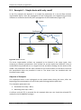
9.2
Example 2 – Combined full basin with meteorological stations ........................................... 71
9.3
Example 3 – Equipped basin with a hydropower scheme..................................................... 84
9.4
Example 4 – Automatic calibration of a model ..................................................................... 97
Bibliography......................................................................................................................................... 106
Acknowledgments ............................................................................................................................... 108
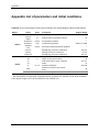
Appendix: List of parameters and initial conditions............................................................................. A.1
RS MINERVE – User’s Manual
Page 5/108
Foreword
RS MINERVE is a software for the simulation of free surface run-off flow formation and
propagation. It models complex hydrological and hydraulic networks according to a semidistributed conceptual scheme. In addition to particular hydrological processes such as
snowmelt, glacier melt, surface and underground flow, hydraulic control elements (e.g.
gates, spillways, diversions, junctions, turbines and pumps) are also included.
The global analysis of a hydrologic-hydraulic network is essential in numerous decisionmaking situations such as the management or planning of water resources, the optimization
of hydropower plant operations, the design and regulation of spillways or the development
of appropriate flood protection concepts. RS MINERVE makes such analyses accessible to a
broad public through its user-friendly interface and its valuable possibilities. In addition,
thanks to its modular framework, the software can be developed and adapted to specific
needs or issues.
RS MINERVE contains different hydrological models for rainfall-runoff, such as GSM,
SOCONT, SAC-SMA, GR4J and HBV. The combination of hydraulic structure models
(reservoirs, turbines, spillways,…) can also reproduce complex hydropower schemes. In
addition, a hydropower model computes the net height and the linear pressure losses,
providing energy production values and total income based on the turbine performance and
on the sale price of energy. A consumption model calculates water deficits for consumptive
uses of cities, industries and/or agriculture. A structure efficiency model computes
discharge losses in a structure such a canal or a pipe by considering a simple efficiency
coefficient.
The RS Expert module, specifically created for research or complex studies, enables in-depth
evaluation of hydrologic and hydraulic results. Time-slice simulation facilitates the analysis
of large data sets without overloading the computer memory. Scenario simulation
introduced the possibility of simulating multiple weather scenarios or several sets of
parameters and initial conditions to study the variability and sensitivity of the model results.
The automatic calibration with different algorithms, such as the SCE-UA, calculates the best
set of hydrological parameters depending on a user-defined objective function.
RS MINERVE program is freely distributed to interested users. Several projects and theses
have used and are using this program for study basins in Switzerland, Spain, Peru, Brazil
France and Nepal. In addition to the research center CREALP and the engineering office
HydroCosmos SA, which currently develop RS MINERVE, two universities (Ecole
Polytechnique Fédérale de Lausanne and Universitat Politècnica de València) collaborate to
improve RS MINERVE and use it to support postgraduate courses in Civil Engineering and
Environmental Sciences. Other collaborations, such as with the Hydro10 Association,
complement and enhance the development of RS MINERVE.
RS MINERVE – User’s Manual
Page 6/108
Chapter 1: Introduction
RS MINERVE is based on the same concept than Routing System II, earlier software
developed at the Laboratory of Hydraulic Constructions (LCH) at the Ecole Polytechnique
Fédérale de Lausanne (EPFL) (Dubois et al., 2000; García Hernández et al., 2007) and used
since 2002 in different projects and theses, such as by Jordan (2007) or Claude (2011).
The software presented hereafter, RS MINERVE, is currently developed by the CREALP and
HydroCosmos SA, with the collaboration of the previously mentioned LCH as well as the
Universitat Politècnica de València (UPV). It has also been used since 2011 in numerous
projects and theses (e.g. García Hernández, 2011).
This first chapter contains the structure of the manual, the procedure to install and update
RS MINERVE and the overview of the RS MINERVE window.
1.1 Document structure
The manual is composed of nine main chapters:
1.
2.
3.
4.
5.
6.
7.
8.
9.
Introduction
Hydrological models
Database
Simulation
Model calibration
Hydraulic structures
RS Expert
RS GIS
Examples of application
In the different chapters, actions to be done by the user are presented in blue.
After the bibliography, the appendix presents in detail the different parameters and initial
conditions of the hydrological models available in RS MINERVE. In addition to this User’s
manual, the reader can also find all model equations and file descriptions in the technical
manual (García Hernández et al., 2015)
1.2 Installation procedure
Proceed as follows to install RS MINERVE on your computer (requires Windows 7 or later
versions of Windows):






Visit the CREALP website: http://www.crealp.ch
Go to Resources -> Software -> RS MINERVE -> Download
Click on Download page: RS MINERVE
Save the file, double-click on Setup.exe (in the Internet browser Downloads frame)
and follow the installation procedure.
Read and accept the Terms and conditions for use of RS MINERVE software.
Click on Install.
RS MINERVE – User’s Manual
Page 7/108
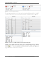
RS MINERVE – User’s Manual
Solver
Data Source
Regulation
Sta ndard
Structures
Ba s e
Description
Objects
Editing tools
Project
Model
Interface
Database
Parameters
and variables
RS MINERVE
Toolbox
Initial Conditions
Parameters
(Graph or values table)
Used to show the
variables of a given
object
Series
- Name
- Zone
- Inputs
- Outputs
Search tool
Object description:
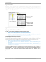
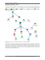
Chapter 1: Introduction
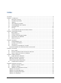
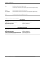
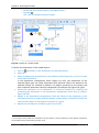
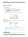
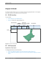
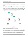
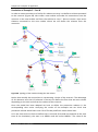
Figure 1 Structure of the RS MINERVE main window
Page 8/108
Chapter 1: Introduction
1.3 Updates
When RS MINERVE is opened and if an Internet connection is available, RS MINERVE
connects to the server to check if a new version is available. If this is the case, the user is
invited to install the new version by accepting the update.
Figure 2 Installation of updates
1.4 Uninstallation procedure
To uninstall RS MINERVE, use the conventional uninstallation procedure in Windows.
1.5 The RS MINERVE main window
The structure of the RS MINERVE main window and the different frames composing it are
presented in
Figure 1.
The Interface frame (
Figure 1) in the middle of the RS MINERVE window allows the visualization of the model
network.
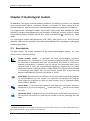
Interaction within the Interface is possible with the mouse.




Use the scroll wheel to zoom in / zoom out
Press the scroll wheel and move the mouse to move the interface window
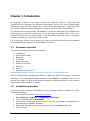
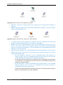
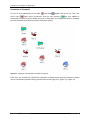
Left click on an object (Figure 3 (b)) -> Select the object and move it in the interface
Double-click on an object (the object is highlighted, Figure 3 (c)) -> Display the Object
description, Series and other corresponding frames (in the right part).
a)
b)
c)
Figure 3 Example of an unselected object (a), after a left click (b) and after a double-click (c)
RS MINERVE – User’s Manual
Page 9/108
Chapter 1: Introduction
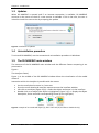
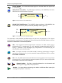
1.6 The Search tool
To facilitate navigation in the main window, the
Search tool (right-frame) allows the user to enter the
name of an object. All corresponding names are listed
and a click on the correct one opens the parent
model and highlights the corresponding object.
Figure 4 The Search tool
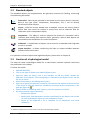
1.7 Settings
The user can access to the settings in the RS MINERVE frame (Figure 5) and can change the
following values:

The units of inputs, parameters and state variables of RS MINERVE (Precipitation,
Temperature, Length, Height,…)

The interpolation method for meteorological values:
o Thiessen polygons: for using the nearest meteorological station
o Shepard method: for values depending on inverse distance weighting

The Potential Evapotranspiration (ETP) method used in the hydrological model. The
ETP can be directly taken from Database, or computed with one of the following
methods:
o Turc
o McGuinness
o Oudin
o Uniform ETP
RS MINERVE – User’s Manual
Page 10/108
Chapter 1: Introduction
Figure 5 RS MINERVE Settings window
The settings are saved in the user’s computer and are kept when the program is opened
again.
1.8 List of keyboard shortcuts and mouse actions
The user can use a list of keyboard shortcuts (Table 1) as well as a list of mouse actions
over the graphics (
Table 2).
Table 1 List of keyboard shortcuts
Ctrl + N
New Project
Ctrl + O
Open Project
Ctrl + S
Save Project
Ctrl + Shift + S
Save as Project
Ctrl + W
Close Project
F5
Start Simulation
Shift + F5
Stop Simulation
RS MINERVE – User’s Manual
Page 11/108
Chapter 1: Introduction
Esc
Back (go to hierarchical higher level),
Cancel object selection (when object type selected in Objects frame)
Space
Switch between Select and Connections
Ctrl + Space
Switch between Select and Transitions (in a Regulation object only)
Ctrl
To select more than one object or series
Table 2 List of mouse actions in graphics
Over the axes
Left click
Right click and move the mouse
Move the scroll wheel
Click on scroll wheel and move the mouse
Double click on scroll wheel
Displace the current view
Zoom in / zoom out
Select the zoom zone
Back to default zoom
Over the time series plot
Left click
Right click and move the mouse
Move the scroll wheel
Click on scroll wheel and move the mouse
Double click on scroll wheel
RS MINERVE – User’s Manual
Date and value of the nearest series point
Displace the current view
Zoom in / zoom out
Select the zoom zone
Back to default zoom
Page 12/108
Chapter 2: Hydrological models
Chapter 2: Hydrological models
RS MINERVE is an object-oriented modeling software. The different processes are modeled
with equation-based objects, presented hereafter in Chapters 2.1 (Base objects) and 2.2
(Standard objects). Hydraulic structures and Regulation objects are presented in Chapter 6.
The implemented hydrological models (Snow-GSM, Glacier-GSM, GR3, SWMM and GSMSOCONT) have been developed within the framework of different research projects, namely
CRUEX (Bérod, 1994), SWURVE (Schäfli & al., 2005) and MINERVE 1 (Hamdi & al., 2003,
2005).
The hydrological models HBV (Bergström 1976, 1992), GR4J (Perrin et al., 2003) and SAC
(Burnash, 1995) are also included in the software RS MINERVE for extending the hydrological
modeling possibilities.
2.1 Base objects
The Base objects are mostly composed of the hydro-meteorological objects. For more
details, see the Technical Manual.
Virtual weather station - It calculates the local meteorological conditions
(precipitation (P), temperature (T) and potential evapotranspiration (ETP)) based
on observed or forecasted data from the database and based on Thiessen or
Shepard interpolations. In addition, the ETP can be also calculated either with a
constant value or from one of the different equations proposed by Turc (1955,
1961), McGuinness et Bordne (1972) or Oudin (2004). The method can be selected
in the Settings (see chapter 1.6). For more details, please refer to the Technical
Manual of RS MINERVE (García et Hernández al., 2015).
Snow-GSM - Simulates the time evolution of the snow pack based on temperature
(T) and precipitation (P). The output is an equivalent precipitation (P eq) and the
snow height (H) proposed as input to other models such as Infiltration (GR3),
Glacier-GSM or SOCONT.
Glacier-GSM - It calculates the volume of melt flow from the glacier based on
temperature (T) and snow height Hsnow (snow melt for Hsnow>0 and ice melt when
Hsnow=0).
Infiltration (GR3) - It determines the part of the gross rainfall which participates in
the runoff as net rainfall (iNet) and the part stored in the soil producing the base
flow.
1
MINERVE: Modélisation des Intempéries de Nature Extrême du Rhône Valaisan et de leurs Effets (Modeling of
Rhone extreme floods in Valais and their consequences).
RS MINERVE – User’s Manual
Page 13/108
Chapter 2: Hydrological models
Runoff (SWMM) - The runoff-based hydrograph is calculated with this object from
a net rainfall (iNet).
GSM (Glacial Snow Melt) - The GSM object combines, in RS MINERVE, the SnowGSM and Glacier-GSM models (Figure 6).
Hsnow, T, Peq
P,T
Q_tot
Figure 6 Composition of the GSM object
SOCONT (SOil CONTribution) - The SOCONT object combines, in RS MINERVE, the
Snow-GSM, Infiltration (GR3) and Runoff (SWMM) models (Figure 7).
ETP
P,T
QGR3
Peq
i net
Q_tot
Qr
Figure 7 Composition of the SOCONT object
The parameters of the SOCONT and GSM objects are the sum of parameters of the objects
composing their combinations. The behavior of the GSM and the SOCONT objects and their
respective combination is therefore equivalent.
HBV - This integrated rainfall-runoff model is based on the HBV model. Using a
precipitation (P), a temperature (T) and a potential evapotranspiration (ETP) as
inputs, it produces a total discharge (Qtot) composed of a run-off flow (Qr), an
interflow (Qu) and a baseflow (Ql).
GR4J - This object is based on the GR4J model, containing 4 parameters. Using an
equivalent precipitation (Peq) and a potential evapotransipration (ETP) as inputs,
an outflow is calculated.
SAC - The SAC-SMA (Sacramento-Soil Moisture Account) object uses an equivalent
precipitation (Peq) and a potential evapotranspiration (ETP) as inputs and provides
an outflow at the outlet of the subbasin.
Channel reaches - The flow is transferred based on the Kinematic and
Muskingum-Cunge (1969, 1991) equations.
Junction - This object allows calculating the addition of different flow inputs (also
coming from hydraulic structures).
RS MINERVE – User’s Manual
Page 14/108
Chapter 2: Hydrological models
2.2 Standard objects
The Standard objects are complementary but generally necessary for feeding, structuring
and calibrating the model.
Time series - Data can be provided to the model as time series (time in seconds).
Data of any type (Flow, Temperature, Precipitation, ETP,...) can be directly
transferred to other objects.
Source - Data can be also loaded from a database. Sources are mostly used to
define flow time series for turbine or pump flow and as reference flow for
calibration (with a Comparator object).
Comparator - This object is used to compare the results of a simulation with a
reference data coming from another object, generally a Source. Both objects are
connected to the Comparator for results comparison.
Submodel - A combination of objects can be saved as a submodel and integrated
as such in a model.
Group Interface - It allows transferring the input or output variables between
different hierarchical levels.
For hydraulic structures objects and regulation objects, please refer to Chapter 6.
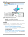
2.3 Creation of a hydrological model
The steps to create a hydrological model for a natural basin (without hydraulic structures)
are presented in this chapter.
To create the model







2
Open RS MINERVE.
Click on the type of object to be added (Objects frame,
Figure 1). With the pencil, click in the Interface to add the object. Repeat the
operation for all objects. If the wrong object is selected in the Objects frame, use the
Esc key to cancel.
Select Connections in the Editing tools frame (
Figure 1) or press the space key to switch, interconnect the objects with blue arrows
in the sense of flow and select the variables(s) concerned by the connections in the
pop-ups (Figure 8). 2
Choose Select in the Editing tools frame or press the space key to switch.
By clicking on each object separately,
o Rename the objects.
o Modify their fixed parameters (such as coordinates for the Station and surface
for main hydrological objects) in the Parameters frame (
o Figure 1). See Appendix 1 for a complete list of parameters and initial
conditions.
In absence of water flow, connect arrows in the sense of information transfer.
RS MINERVE – User’s Manual
Page 15/108
Chapter 2: Hydrological models
o Define the Zone of each object in the Object frame (
o Figure 1). 3
Use “Tab” to validate the Zone number.
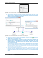
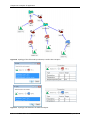
Figure 8 Example of a simple model
To define the Parameters of the model objects:

Click on


Figure 1).
Select an Object type and a Zone Id in the Selection frame (Figure 9). Use Ctrl to select
more than one Zone ID.
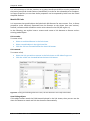
In the Parameters management frame (Figure 10, left), the parameters of the
selected object type are listed. Parameters with identical value in all objects of the
selected zone(s) are checked by default. The objects contained in the zone(s) and
their respective parameter values are displayed in the Objects list (Figure 10, right).
Define the parameters to be calibrated, i.e. uniformly modified, by checking and
unchecking the parameters in the Parameters management frame (the [x] column,
Figure 10, left).
Modify in the Parameters management frame the values of the Parameters to be
calibrated and click on Apply selected changes. (Alternatively, individually modify the
values of each object in the Objects list (Figure 10, right)).
Repeat the procedure for all object types in each zone.



Parameters in the Parameters and Variables frame (
3
The concept of Zones allows the modification of a parameter or initial condition to all the objects contained in
the selected zone(s) by attributing a unique value.
RS MINERVE – User’s Manual
Page 16/108
Chapter 2: Hydrological models
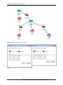
Figure 9 Selection frame
Figure 10 Left: Parameters management frame; Right: Objects of the selected zone(s) and their
parameters
To define the Initial Conditions:

Click on Initial Conditions in the Parameters and Variables frame (


Figure 1).
Proceed in a similar way than for the Parameters definition to modify all the Initial
Conditions.
Initial conditions are generally not known precisely. Approximated values can be entered to
improve the simulation results. Final conditions of a previous simulation ending at the start
time of the period of interest can be used as current initial conditions to improve the results.
To save the project:

Click on Save in the Project frame (


Figure 1).
Define the file name and save.
2.4 Exportation of a submodel
Combinations of objects can be exported and later imported as Submodel objects in a
complete model. This allows the structuration of the model by organizing it in different
hierarchical levels.

Add a
Group Interface to the combination of objects to be exported.
4
4
Group Interfaces are required to assemble a submodel with the upper hierarchical level. It allows transferring
the input and/or output variables.
RS MINERVE – User’s Manual
Page 17/108
Chapter 2: Hydrological models

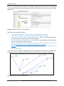
Link the output object of the model (Junction in Figure 11) to the Group Interface.
Select the link(s) to be created in the pop-up (Flow in the example of Figure 11). 5
Figure 11 Addition of a Group Interface to the combination of objects to be exported as submodel






Export the active model with the Export button in the Model frame (
Figure 1). 6
Create a new project with the New button in the Project frame. 7
Import the Submodel with the Import button in the Model frame.
Open the Submodel with a right-click on it. The model previously created appears.
Return to the upper hierarchical level with the Back button (Model frame) or by
pressing the Esc button.
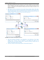
 Add a Junction object and link the Submodel to the new Junction (Figure 12). In the
example of Figure 12, the flow of the new Junction now corresponds to the flow of
the Junction in the Submodel.
Figure 12 Link the Submodel to a Junction
At the same time, if a Submodel receives also an input from upstream, a second Group
Interface has to be added in the Submodel and linked to the object receiving the incoming
variables. Group Interfaces can support more than one variable as input and/or as output.
Submodels can also be created by adding an empty
Submodel object 8 and then adding
the adequate objects in the Submodel (opened with a right-click). In a similar way, objects
can be added to or deleted from imported Submodels.
Modifying the Zone of a Submodel modifies the zone of all the objects contained in the
Submodel.
5
If only one link can be created, it is selected by default. If more than one link is possible, none is selected.
During the exportation, only the elements contained in the active hierarchical level, including all the
submodels and objects, are considered. Hierarchically higher elements are not exported.
7
Or, alternatively, open a project with Project -> Open.
8
By selecting Submodel in the Standard objects frame and adding the object in the Interface.
6
RS MINERVE – User’s Manual
Page 18/108
Chapter 2: Hydrological models
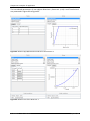
2.5 Model conversion
The conversion between different hydrological models is possible with the button
of the Model frame (Figure 13).
Figure 13 Model frame
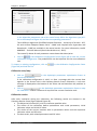
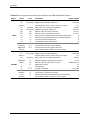
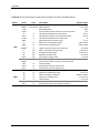
The model conversion is direct for hydrological model conversions presented in Table 3. For
achieving the conversion, initial and final hydrological model types are selected. Then, the
zone(s) and the object(s) to convert are chosen (Figure 14).
In the current version, only the parameter A (Surface) is transferred to the new model. All
other parameters are fixed to the by default values of each model.
Figure 14 Example of a conversion between HBV and SOCONT
If the converted model does not need all inputs, a message informs that one of the inputs is
deleted, as presented in Figure 15 for the input Temperature.
Figure 15 Example of a conversion between a model HBV and SAC, where the input Temperature is
deleted
Finally, if the converted model needs more inputs than the original one, a message informs
that one or several inputs need to be added, as presented in Figure 16 for the input
Temperature. In that case, the link between the stations and the model needs to be replaced
(or, if the data comes from a different Station or Time Series, a new link has to be added).
RS MINERVE – User’s Manual
Page 19/108
Chapter 2: Hydrological models
Figure 16 Example of a conversion between a model SAC and HBV, where the input Temperature has
to be implemented by the user
Regarding the outputs, the total discharge (Qtot or Q depending on the model) is directly
linked to the downstream object after the conversion.
If any other discharge is linked downstream, e.g. the Qr in the SOCONT model to a junction,
the link is deleted after conversion.
RS MINERVE – User’s Manual
Page 20/108
Chapter 2: Hydrological models
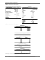
Table 3 Direct conversions between objects
Object
Glacier-GSM
GR3
Inputs
P and T
P and ETP
Object
Inputs
GSM
P and T
GR4J
P and ETP
SAC
P and ETP
SWMM
P
SWMM
P
No direct conversions
GSM
P and T
GSM
P and T
GSM
P and T
GR3
P and ETP
GSM
P and T
HBV
P, T, ETP
GR4J
P and ETP
SAC
P and ETP
SWMM
P
GSM
P and T
GR3
P and ETP
GSM
P and T
SOCONT
P, T, ETP
GR4J
P and ETP
SAC
P and ETP
SWMM
P
GR3
P and ETP
SAC
P and ETP
SWMM
P
GR3
P and ETP
GR4J
P and ETP
SWMM
P
SOCONT
HBV
GR4J
SAC
P, T, ETP
P, T, ETP
P and ETP
P and ETP
RS MINERVE – User’s Manual
Page 21/108
Chapter 3: Database
Chapter 3: Database
The different input data as well as exported results are managed within a database. The RS
Database tool, accessible from the RS MINERVE window, is used to create or edit the
database linked to the active model.
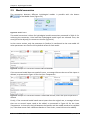
3.1 The RS Database tool
The RS Database tool window appears when a database is created (
edition ( Open and then Edit).
File
database
File
dataset
Edition
RS
Database
New) or opened for
Selected component
description
Database
Group
Dataset
Station
Sensor
Database
Components
Data (Graphics or table)
Figure 17 The RS Database window
The database structure is organized in five hierarchical levels, listed hereafter.
 Database Description of the database, complete set of data
 Group Separation based on category of data (Measures, Forecasts, Simulations,…)
 Dataset Set of data of common type (Meteo data, Flow data,…) 9
 Station Information about the station (name and coordinates)
 Sensor Description of the sensor (name, units and data)
9
9
Definition and use of Groups and Datasets can also be done in a different way by the user.
RS MINERVE – User’s Manual
Page 22/108
Chapter 3: Database
3.2 Creation of a database
The creation of a new database can be achieved following next steps:
 Click on New in the Database frame (
 Figure 1) and save the new database. The RS Database window is opened (Figure 17).
 Create the components of the different hierarchical levels of your database by using
the Add button (Edition frame).
 For the stations, give an adequate name and enter the coordinates.
 For each sensor:
o Define the Description (name), Category, Unit and Interpolation method.
o Select the “Values” tab and add the data with the
Paste button (after
copying them from any spreadsheet program).
 Save the database and close the RS Database viewer.
The data can be managed (exported or imported) as database or as dataset.
To manage a database, proceed as follows:
 To save a database: Click on the Database component -> File database -> Save as.
 To load another database in RS Database:
o Close RS Database
o Then, in the RS MINERVE window, click on Close in the Database frame.
o Click on Open in the Database frame to open the new database.
o Click on Edit in the Database frame to open the new database in RS
Database.
To manage a dataset, perform as follows:
 To export a dataset: Click on the Dataset component -> File Dataset -> Save
 To import a dataset: Click on a Group component -> File Dataset -> Import
If a dataset contained in a database is also stored separetely as a dataset (not only in the
database), both have to be saved (File database -> Save; File dataset -> Save) to properly
modify all the files!
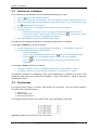
3.3 Data format
For copying series values in a sensor, two columns are necessary. The first column contains
the data in one of these formats:
 dd.mm.yyyy
 dd.mm.yyyy hh:mm
 dd.mm.yyyy hh:mm:ss
The second column contains the values of the series (example in Figure 18).
Figure 18 Example of data format to use in the sensors
RS MINERVE – User’s Manual
Page 23/108
Chapter 3: Database
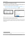
3.4 Connection of a database to a model
Once the database is created, links between the model and the database have to be
implemented. The Data source frame (Figure 19, left), located in the main interface and
available only when a database is opened, is used for this purpose.
 Define for the Station and the Source the corresponding Group and DataSet.
 For the Source objects, define in the Object description frame the correct station
under the Select from database button (Figure 19, right). 10
The name of the station appears under Station identifier and is stored in the model when the
model is saved.
Figure 19 Left: The Data Source frame; Right: Definition of the station for objects Source
Interaction between the database and the active model
Modifications of the database in RS Database (without saving them!) are taken into account
during simulations of the active model. However, when the database is closed, only saved
changes will be applied to the database. Therefore, proper saving of the modifications is
recommended.
10
Source objects have to be linked to another object to define the type of output (and corresponding units)
before the link to the station can be defined.
RS MINERVE – User’s Manual
Page 24/108
Chapter 4: Simulation
Chapter 4: Simulation
4.1 Run a model
Before solving a model, its validity has to be verified.
 Click on the Validation button. A Pre-Simulation report is generated (right-frame).
In case of Fatal error(s): Correct your model consequently. 11
In case of Warning(s): Proceed to adequate modifications if required.
In case of Note(s): Consider the message(s) and go ahead.
 In the Solver window (
 Figure 1), define the simulation period, simulation time step and recording time step
(Figure 20).
Figure 20 The Solver window
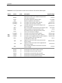
The time interval for the simulation time step and recording time step can be modified
accordingly to Table 4.
Table 4 Possible time intervals for simulation and recording time steps
Simulation time step




Seconds
Minutes
Hour
Day
Recording time step





Seconds
Minutes
Hour
Day
Month

Click on Start. At the end of the computation, a Post-Simulation report (right frame)
provides a summary of the simulation with potential warning(s).

Visualize the obtained results by selecting each object in the Interface and using the
Graphs tool in the Object frame (

Figure 1). Select the variable(s) of interest in the list (use Ctrl to select more than one
series).
11
During the Validation process, the model is verified. In particular, a Fatal error is generated for each missing
required object’s input (absence of interconnection from upstream).
RS MINERVE – User’s Manual
Page 25/108
Chapter 4: Simulation
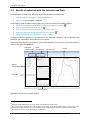
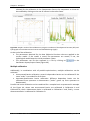
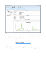
4.2 Results visualization with the Selection and Plots
A combination of results can be visualized in the Selection and Plots tool.

Click on Selection and plots in the Toolbox frame (

Figure 1). A new window is opened.
In the Objects and variables frame (Figure 21), all the variables are listed by objects.





Check in the Objects and variables frame the variable(s) to draw.
Click on Plot to plot the listed series. 13
Give a name to the active selection in the Selections list.
Export the selection using Selections frame -> Export. 14
Import a selection using Selections frame -> Import.
12
A second selection appears in the Selections list. Different selections can be defined and
saved for the exploitation and analysis of the results.
Note that when Selection and Plots is opened, RS MINERVE is not active. Close Selection and
Plots to use again RS MINERVE.
Series
Selections
import/export management Selections list
Graph
Objects
and variables
Series list
Source of data
Figure 21 The Selection and Plots window
12
Variables of two different units can be drawn simultaneously (second axis).
Use the mouse to visualize data values (press left button), move (press right button), zoom (press scrollwheel) or fit to view (double-click on scroll-wheel). Zoom and fit to view can be also realised onto the axes.
14
Selections are saved in a text file with the *.chk format.
13
RS MINERVE – User’s Manual
Page 26/108
Chapter 4: Simulation
4.3 Export / Import of results to a database
Results of a simulation can be saved to the database as a dataset of time series.
 Select Export in the Database frame (
 Figure 1) in the RS MINERVE main window.
 Define the name of the dataset and choose between:
o Add the dataset to an existing Group.
o Create a new Group.
 Export with OK. 15
You can now visualize your results in the database (cf. Chapter 3). Once exported, results can
be imported into the model. Importing a dataset of series replaces the current time series
(results of a simulation) of all concerned objects.
 Select Import in the Database frame.
 Select the Group and the Dataset of time series to import and click Ok.
Exported results can also be visualized in the Selection and Plots tool.
 Open Selection and Plots tool (Toolbox frame -> Selection and plots).
 In the Source of data, check the Database source (Figure 21), then select in the
combo the Group containing the dataset of time series.
 Select the dataset of time series to be drawn.
 Click on Plot in the Series frame.
15
By activating Only selected series, only the series corresponding to the last active Selection in the Selection
and Plots are exported.
RS MINERVE – User’s Manual
Page 27/108
Chapter 5: Model calibration
Chapter 5: Model calibration
The calibration process aims to progressively improve the model to fit the simulated data to
the reference data (e.g. the observations) by iteratively adjusting the object’s parameters.
5.1 Single sub-basin calibration
To proceed to the calibration, observed data are required as comparison basis for the
simulated data. Sites of measure stations generally define outlets of sub-basins since they
represent the location of comparison (simulated data vs. observed data). 16
For simplicity, division into zones generally respects the sub-basin’s division. However, this is
not compulsory and a zone can correspond to several sub-basins or one sub-basin can be
divided into several zones. In this first part (Chapter 5.1), it is assumed that the sub-basin is
composed of a single zone.
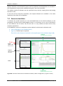
Model’s performance evaluation
Before adjusting the parameters, the current performance of the model is evaluated.
 Click on the
Comparator object which has been added and connected as
presented in Figure 8.
 In the Series frame (Figure 22), select Qreference and Qsimulation (use Ctrl to select both).
 Visualize the actual results:
o In the Series frame, both curves are plotted together under Graphs.
o In the Comparator frame, seven performance indicators are provided (read
the Technical Manual for more information (García Hernández et al., 2015)).
 Nash coefficient
 Nash-ln coefficient
 Pearson Correlation Coefficient
 Bias Score
 Relative Root Mean Square Error
 Relative Volume Bias
 Normalized Peak Error
Manual parameters adjustment
Based on the current model’s performance, object’s parameters can be adjusted to improve
the next run’s performance.
 Click on Parameters in the Parameters and variables frame (Figure 22).
 Select in the Selection frame (Figure 22) the type of object to be modified and the
corresponding zone. See Chapter 2 for complete procedure.
16
Other factors are also considered during the basin division such as reservoir locations or river junctions.
RS MINERVE – User’s Manual
Page 28/108
Chapter 5: Model calibration
 Modify the selection (checks) of parameters in the Parameters Management frame
to select only the ones to be calibrated (i.e. to be uniformly modified).
 Modify the values of the selected parameters and click on Apply selected changes.
Parameters are modified in the listed objects.
 Proceed in a similar way for all object types.
 Modify also the initial conditions to fit better the reference data.
Parameters
and variables
Comparator
Selection
Series
Parameters management
and objects
Figure 22 Frames used for the calibration
 After running the model, analyze the results in the comparator and modify again the
parameters when necessary.
The procedure is iterative until the simulation results are considered sufficiently satisfying
for a specified zone.
Parameters and Initial conditions can be exported to be, later, imported again. Use Export P
and Import P for the parameters and Export IC and Import IC for the initial conditions in the
Parameters and variables frame (Figure 22). The parameters or initial conditions can be
saved as .txt file or also as .xlsx file with one sheet per object type.
Automatic parameters adjustment
An automatic calibration can be also achieved thanks to a specific module developed in
RS Expert. Please the chapter 7.1 for more information.
RS MINERVE – User’s Manual
Page 29/108
Chapter 5: Model calibration
5.2 Complete basin calibration
When a basin is composed of many sub-basins, the calibration has to be progressively
achieved from upstream to downstream in the basin. By proceeding as such, contributions
from the upstream calibrated sub-basin(s) are considered as input(s) to the downstream
sub-basin on which the calibration is performed. Parameters are modified for the concerned
sub-basin to obtain the best possible results at the outlet of the sub-basin. The calibration
module (Chapter 7.1) can realize multiple calibrations for calibrating these complex basins
from upstream to downstream.
Depending on the quality of the simulation results, inputs from upstream sub-basins can be
replaced in the calibration process by observed data at the entrance of the sub-basin being
calibrated.
RS MINERVE – User’s Manual
Page 30/108
Chapter 6: Hydraulic structures
Chapter 6: Hydraulic structures
Chapters 1 to 5 have presented the different steps to create a hydrological model without
any hydraulic structures. Chapter 6 explains how structures like reservoirs, turbines or
spillways are implemented in RS MINERVE.
Hydraulic structures are listed in Chapter 6.1 and objects used for automatic regulation are
presented in Chapter 6.2.
6.1 Hydraulic structure objects
Reservoir - Water level and volume evolution are simulated based on a “LevelVolume” relation and an initial reservoir level.
HQ - Based on a level-discharge relation, it allows integration of level-based
outflows to reservoirs (such as spillways, gates, orifices,…).
Turbine - It calculates the turbine or pump flow from a reservoir, based on a
Wanted Discharge defined in a Source or in a Time Series.
TurbineDB - The TurbineDB object works as the Turbine object but is directly
based on data provided by the database. It is equivalent to the combination of a
turbine and a source.
Hydropower - This object calculates the power and the revenue, normally
produced by a turbine, depending on the discharge and on the reservoir level.
Diversion - This object is used to simulate the separation of flow based on an
“Inflow - Diverted flow” relation. It can be used as a hydrological object but is
mostly used as a hydraulic function.
Consumer - This object simulates the consumed discharge of a user (e.g.: a
village or an agricultural field) based on a series from a database or from a
uniform demand.
Structure efficiency – This object computes effects of discharge losses in a
structure like a canal or a pipe based on an efficiency coefficient.
RS MINERVE – User’s Manual
Page 31/108
Chapter 6: Hydraulic structures
6.2 Regulation objects
Sensor - Sensors are connected to other objects (generally reservoirs) from
which they measure a particular variable to compare it to user predefined
thresholds. In the case of a reservoir, water level or volume can be monitored.
Regulation - It allows loading the Regulation interface in which regulatory
models with different States are developed.
State - In a Regulation, several State objects can be included to adapt the
operations based on the situation. Only one State can be active in a Regulation.
Transfer from one State to another are based on threshold values monitoring
provided by Sensors.
6.3 Addition of a Hydropower scheme
This chapter presents a general example for the construction of a hydropower scheme,
including a reservoir with a hydropower plant, a turbine and a spillway.
Addition of a reservoir
To add a reservoir:
 Select the object Reservoir in the Structures objects frame (Figure 23) and add it in
the Interface.
 Link the output of the upstream sub-basin (object Junction in Figure 23) to the
Reservoir.
Structures
objects
Regulation
objects
Reservoir
Series
Data
source
Initial
conditions
Figure 23 A regular model with a reservoir
 Double-click on the Reservoir object. The Reservoir, Series and Initial Conditions
frames are opened (Figure 23).
 In the Series frame, select the H-V series and open the Values tab.
 By default, the table is empty. Insert the corresponding Height-Volume (H-V) relation
for the reservoir.
 Define an initial water elevation (HIni) in the Initial conditions frame.
RS MINERVE – User’s Manual
Page 32/108
Chapter 6: Hydraulic structures
Alternatively to the last point to define the initial water elevation of the Reservoir, a time
series can be saved in the database with a sensor of Category Altitude and Unit masl. For
each simulation, RS MINERVE will then search and interpolate the initial condition from the
added time series. To link the Reservoir with the sensor, first select in the Data Source frame
the corresponding Group and Dataset.
Then, in the Reservoir frame (right part), click on the Select station from Database button
and define the correct station in the Station drop-down list (only stations containing a sensor
with appropriate units are listed). The value in the Initial conditions frame will change after
every simulation to the value interpolated from the time series.
Once a reservoir is implemented, outputs of the reservoir have to be defined. Water from a
reservoir can be exited through different ways. A combination of Turbine (or TurbineDB) and
Hydropower objects are used to simulate the use of water for hydropower production.
Regulations are generally used to automatize the operation of Turbine and TurbineDB
objects. Finally, HQ objects generate discharges based on elevation-discharge relations. 17
All these objects can be used independently and cumulatively. For example, several turbines
can be placed in parallel with one or several TurbineDB(s), HQ object(s) and/or Regulation(s).
None of them is imperative.
Addition of a TurbineDB object
The TurbineDB object is based on data from a database. Thus, before adding a TurbineDB,
data have to be added to the database
 Open a database (see Chapter 3) and create a station with a sensor of category Flow.
Modify the description and insert data for the TurbineDB outflow in the Values tab.
The TurbineDB object is then added.
 Select the object TurbineDB in the Structures objects frame (Figure 23) and add it in
the Interface. Add also a Junction to which outflow(s) from the Reservoir will be
linked to.
 Switch to Connections (Editing Tools frame-> Connections or use the space key) and
link the Reservoir to the TurbineDB object and the TurbineDB object to the Junction
(Figure 24).
Figure 24 Addition of a TurbineDB and a junction
17
As outputs from the Reservoir are defined by downstream objects, output flows (Qs) are considered as an
Input to the Reservoir in terms of information flow. The corresponding water is thereby withdrawn from the
13
stored volume. This implies that at least one output flow has to be defined to validate the model (See
).
RS MINERVE – User’s Manual
Page 33/108
Chapter 6: Hydraulic structures
 In the Data Source frame (Figure 23), select for the line HPP 18 the Group and
DataSet corresponding to the sensor created in the database.
 Double-click on the TurbineDB object to open the TurbineDB frame (right-side). Then,
click on the
Select station from Database button and define the corresponding
station in the Station drop-down list. The link between the TurbineDB object and the
database is now operational.
The TurbineDB object is ready for use.
Addition of a Hydropower object
The Hydropower object calculates the power and the revenue produced by the discharge of
the turbine from the reservoir. The results depend on the discharge and on the reservoir
water level.
 Select the object Hydropower in the Structures objects frame (Figure 23) and add it in
the Interface (Figure 25).
Figure 25 Addition of a Hydropower object
As the power produced in the hydropower plant depends on the water level in the reservoir
and on the discharge of the turbine, the links between the Hydropower and the Reservoir
objects, and between the Hydropower and the Turbine DB objects must be created (Figure
26).


18
Link the Reservoir to the Hydropower object so the water level information can be
transferred to the Hydropower object.
Link the TurbineDB to the Hydropower object so the discharge variable can be
transferred to the Hydropower object.
Short for HydroPower Plant, which includes the TurbineDB and the Hydropower objects.
RS MINERVE – User’s Manual
Page 34/108
Chapter 6: Hydraulic structures
Figure 26 Links between the Hydropower object and the Reservoir and with the TurbineDB
 Double-click on the Hydropower object to open the Hydropower frame (right-side).
Then, click on the
Select station from Database button and define the
corresponding station which contains the "Electricity price" series in the Station dropdown list. The link between the Hydropower object and the database is now
operational.
 In the Series frame, select the Q- (discharge-efficiency) series and open the Values
tab. Insert data for the Q- relation (manually or copied from a spreadsheet).
 In the Parameters frame, introduce the features of the hydropower plant. In
particular the following parameters must be specified: the hydropower plant altitude
(Zcentral) in masl; the length of the pipe (L) in m; the diameter of the pipe (D) in m;
the Roughness (K) in m; the kinematic viscosity () in m2/s; and the default price of
electricity, only used if no data exists in the database.
The Hydropower object is ready for use.
Addition of an HQ object
HQ objects are used to define level-discharge relations to implement structures such as
spillways, orifices or sluice gates. For illustration purpose, an HQ object is used as a spillway
in the following procedure.
 Select the HQ object in the Structures objects frame (Figure 23) and add it in the
Interface.
 Link the Reservoir to the HQ object and the HQ object to the Junction (Figure 27).
RS MINERVE – User’s Manual
Page 35/108
Chapter 6: Hydraulic structures
Figure 27 Addition of a spillway

Double-click on the HQ object. In the Series frame, select the H-Q series and open the
Values tab. Insert data for the H-Q relation (manually or copied from a spreadsheet).
The HQ object is ready for use.
Simulation with implemented structures
Several structures can be added in parallel as illustrated in Figure 27. When all objects are
created, the model linked to the database and validated, start the simulation (Chapter 4.1).
Discharges through the different objects can then be visualized by clicking on each object
(Chapter 4.1) or within the Selection and Plots tool (Chapter 4.2).
It is important to remember that discharges generated by HQ objects are defined by the
water level in the reservoir. Below a certain level, no discharge is produced. This is not the
case of the TurbineDB objects that withdraws from the reservoir the discharges defined in
the database, without checking if water is available or not in the reservoir. This might result
in a negative volume in the reservoir (a warning is generated in the Simulation report). In
order to generate discharges only when the water is actually available, Regulation objects
are necessary.
6.4 Implementation of a regulation
Regulation objects allow the definition of automatic rules to switch between different States
depending on the actual conditions in the system. A State object is similar to a submodel
since several objects can be introduced in it as a function of the demands (turbine, pump,
diversion, etc.). A typical example of regulation is the implementation of a turbine law as a
function of the water level in the reservoir.
RS MINERVE – User’s Manual
Page 36/108
Chapter 6: Hydraulic structures
One or several inputs/outputs can be considered in or produced by a State objet. The
definition of the active State is carried out as a function of the user predefined thresholds
values monitored by the Sensor objects.
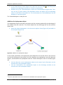
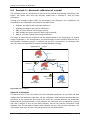
Addition of a regulation
The complete procedure to add and implement a Regulation is detailed hereafter. For
illustration purpose, consider two possible States (“Turbine On” and “Turbine Off”) for the
turbine of the previous example: the turbine should turn off if the water level at the
reservoir falls below 1503 [masl], and turn back on when the water level exceeds 1506
[masl], and so on.

Delete the Turbine DB object of the previous example. Select the Regulation object in
the Regulation objects frame (Figure 23) and add it in the Interface. Add a Sensor and
link the Reservoir to the Sensor (Figure 28).
Figure 28 Objects creation for a Regulation

Double-click on the Sensor. In the Thresholds frame, enter the different threshold
(altitude) values in the Values column (Figure 29). The identifiers (Id) are
automatically created for each entered value.
Figure 29 Example with two threshold values
Sensor objects monitor the user predefined threshold values. For each simulation time step,
the threshold values are compared to the actual value of the monitored variable. Each
threshold value is then characterized by Over or Below the actual level.
 Open the Regulation with a right-click. The empty Regulation interface is opened.
 Add two Group Interfaces and two State objects (Figure 30). 19 Rename the State
objects to give them an explicit name ("Turbine On" and "Turbine Off", for instance).
19
Objects in the Regulation interface cannot yet be interconnected. Group Interfaces have first to be added in
the State objects and connected to other objects.
RS MINERVE – User’s Manual
Page 37/108
Chapter 6: Hydraulic structures
Figure 30 Objects creation in the Regulation interface
 Open the "Turbine On" State object with a right-click. The empty State interface is
opened.
 Add two Group Interfaces and the desired combination of objects. For this example,
add a TurbineDB (Figure 31).
Figure 31 Objects creation in the "Turbine On" State interface
 In the Data Source frame (Figure 23), select for the line TurbineDB the Group and
DataSet corresponding to the sensor created in the database.
 Double-click on the TurbineDB object to open the TurbineDB frame (right-side). Then,
click on the Select station from Database button and define the corresponding
station in the Station drop-down list. The link between the TurbineDB object and the
database is now operational.
 Interconnections between the TurbineDB and both Group Interfaces have now to be
added. One of them will ensure the connection from upstream objects, the second
one to downstream ones.
o For the Interface 1, connect it to the TurbineDB (water flow direction, as
shown in Figure 32). In the Variable selection pop-up, select the link from the
TurbineDB to the Group Interface (information direction).
As the water flow from Reservoir is defined by the TurbineDB, the information
is transferred in the upstream direction from the TurbineDB to the Reservoir
trough the Group Interface.
o For the Interface 2, link the TurbineDB to the Group Interface. In the Variable
selection pop-up, the link from the TurbineDB to the Group Interface is
preselected. Create the link with Ok.
In that case, both information and water flow are in the downstream direction
(from the TurbineDB to the Group Interface).
RS MINERVE – User’s Manual
Page 38/108
Chapter 6: Hydraulic structures
Figure 32 Links creation between the TurbineDB and the Group Interfaces

Return to the upper hierarchical level (Regulation Interface) with the Back button
(in the Model frame) or press the Esc button.
 Open the second State object ("Turbine Off") with a right-click. An empty State
interface is opened.
 Add two Group Interfaces, and a Turbine with a Time Series. Interconnect the Time
Series to the Turbine (Figure 33).
Figure 33 Objects creation in the "Turbine Off" State interface

Double-click on the Time Series. In the Series frame, click on Serie and open the
Values tab. Enter a series of data with time [seconds, starting from 0] and QWanted
[m3/s] as presented in Figure 34. 20 21
20
Time series are entered with time in seconds. The second 0 corresponds to the start time of the simulation.
Consequently, a Time series can be used for different periods of simulation.
21
If the Times series does not completely cover the period of simulation, the last value of the series is
constantly applied for the uncovered part. If the series varies with time, complete coverage of and adequate
correspondence with the period of simulation has to be ensured.
RS MINERVE – User’s Manual
Page 39/108
Chapter 6: Hydraulic structures
Figure 34 Time series data for the “Turbine off”
 Interconnections between the Turbine and both Group Interfaces have now to be
added, as shown in Figure 35. One of them will ensure the connection from upstream
objects, the second one to downstream ones.
Figure 35 Links creation between the Turbine and the Group Interfaces
 Return to the upper hierarchical level (Regulation Interface) with the Back button
(Model frame) or press the Esc button.
 Switch to Connections using the space key. Links between Group Interfaces and
States will now be created. Similarly to the logic in the State objects, one Group
Interface ensures the information exchange with upstream objects, the other one
with the downstream ones.
For the first Group Interface, the one connecting the regulation with the upstream
part of the model (Interface 1 in Figure 36), connect it to the first State (arrow in
water flow direction). The link to be created transfers the information (the TurbineDB
flow) from State to the Group Interface.
 Connect the same Group Interface to the second State. Ensure that the name in the
drop-down list in the Variable selection pop-up is the same as for the first State
(without the indication "(New)" as the target of the link Q up of TurbineDB 4 already
exists).
RS MINERVE – User’s Manual
Page 40/108
Chapter 6: Hydraulic structures
Both States sending to the same reference in the Group Interface, only one variable
will be available in the higer hierarchical level. As one and only one State can be
active in a Regulation, this variable will always have one and only one value in the
Regulation object.
 Both States are then connected to the second Group Interface (Figure 36). Again,
both States point to the same link target (Q down of TurbineDB in the example) in the
output Group Interface, this is why the first State to be connected will have the
indication “(New)” in the dropdown menu and the second not.
Figure 36 Links creation in the Regulation interface
 One more important operation in the Regulation is the definition of the States
transfer rules. To do so, click on Transitions in the Editing tools frame or use
Ctrl+space keys. The State transfer mode is entered: previously created links are
hidden and only both States are visible.
 Link with Transition arrows the two States, as illustrated in Figure 37.
RS MINERVE – User’s Manual
Page 41/108
Chapter 6: Hydraulic structures
Figure 37 Transition links creation between States
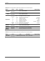
Transitions rules are defined in each Transition arrow based on threshold values monitored
by the Sensor objects. Table 5 presents the Operators used to define these automatic rules.
Adequate use of the “…and” and “…or” functions allow the definition of combined rules.
Table 5 Operators used for automatic rules definition
Operator
>= than
< than
and >= than
and < than
or >= than
or < than

Definition
Bigger than or equal to
Smaller than
…and "bigger than or equal to"
…and "smaller than"
…or "bigger than or equal to"
…or "smaller than"
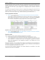
Using the operators presented in Table 5 and the threshold values defined in the
Sensor used to monitor the Reservoir (see Figure 29), define transfer rules by clicking
on the Transitions arrows and filling the cells in the Transition frame. Figure 38
provides an example of simple rules to switch between Turbine On and Turbine Off.
Figure 38 Example of transition rules in a Regulation. In the example, if the water level reaches 1506
[masl], the State Turbine On will be active as long as the level exceeds 1503 [masl]. If the level goes
below 1503 [masl], the State Turbine Off will then be activated as long as 1506 [masl] is not exceeded
in the reservoir, and so on.
RS MINERVE – User’s Manual
Page 42/108
Chapter 6: Hydraulic structures
Before exiting the Regulation, the Initial state has to be defined in the Regulation frame
(right). In the drop-down list, select the State to be active at the beginning of the simulation.
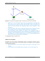
 Return to the upper hierarchical level (complete model) with the
Back button
(Model frame) or press the Esc button.
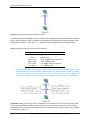
 Link the Reservoir to the Regulation and the Regulation to the Junction (see Figure
39).
Figure 39 Connection of the Regulation with the upstream Reservoir and the downstream Junction
The Regulation object is ready for use.
Simulation with the regulation implemented
Once the two objects (HQ and Regulation) are implemented, validate the model and start
the simulation. Results can be visualized by double-clicking on each object or by using the
Selection and Plots.
RS MINERVE – User’s Manual
Page 43/108
Chapter 7: RS Expert
Chapter 7: RS Expert
In this chapter, the four RS Expert modules are presented:
 Automatic calibration of hydrological model parameters;
 Stochastic simulation
 Time-slices simulation;
 Scenario simulation.
7.1 Automatic calibration
The complexity of a hydrological model calibration increases with the number of parameters
to calibrate. The search for optimal values of calibration parameters can be made manually
to a reasonable number of parameters. But in general, for large basins including hundreds or
thousands of parameters, it is essential to have an automatic calibration tool.
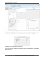
In RS MINERVE, an automatic calibration can be realized in the Hydrological calibration tool
(Figure 40).

Click on RS Expert in the Toolbox frame (

Figure 1). The RS Expert is opened (Figure 40). By default, the Hydrological calibration
interface is showed.
Note that when RS Expert is opened, RS MINERVE is not active. Close RS Expert to use again
RS MINERVE.
Calibration configuration
Different types of calibration can be achieved for an optimization:
 Regular calibration: One or more zones with a unique downstream gauged station,
calibrated with the same parameters for all zones.
 Calibration per zone: One or more zones with a unique downstream gauged station,
calibrated with different parameters per zones.
 Regional calibration: One or more zones with several downstream gauged station,
calibrated with the same parameters for all zones.
The creation of a new calibration configuration can be realized following next steps
(corresponding to the black boxes in the Figure 40):
 In the Selection frame (Figure 40), select the object types to calibrate: press
simultaneously Ctrl on keyboard and left click on the object types. Then define the
corresponding zone(s) by clicking on the Zone Id number(s).
All the objects corresponding to the selected object types and zone(s) appear in the
Models frame (Figure 40). The correspondent parameters are shown in the
Parameters frame (Figure 40).
 In the Parameters frame (Figure 40), select the parameters to calibrate. For each of
them, define their minimum and maximum possible values (Min and Max columns)
RS MINERVE – User’s Manual
Page 44/108
Chapter 7: RS Expert

and the value to be used for the first iteration of the calibration (From model, Defined
value or Random value).
If more than one zone has been selected (Selection frame), a column Values per zone
appears in the table. For the parameter(s) selected for calibration, a box appears in
this column. If the box is checked, the calibration for the parameter will consider a
different value for each zone. If not, the same value will be considered for all zones in
the concerned calibration.
Parameters can be imported in the model by clicking on
import/export frame (Figure 40).
in the Parameters
In the Comparators frame (Figure 40), select the comparator(s) whose the observed
discharges will be used for the calibration (press simultaneously Ctrl on keyboard and left
click on the comparators name to select more than one). If more than one comparator is
selected, all will be taken into account in the objective function with the same weight.
Calibration configuration
Parameters
(Import/export)
Comparators
Models
(To calibrate)
Parameters
(To calibrate)
Selection
(Model and
zones)
Objective
function OF
(Indicators
weight)
Hydrologic
parameters
optimization
(Runtime and
algorithm
parameters)
Summary results
Graphic results
Figure 40 Interface of the Hydrological calibration module (in black: configuration; in green: results)
 Define the weight of each indicator to determine the objective function in the
Objective Functions (OF) frame. Its total weight appears in the cell at the top of the
frame.
 In the Solver tab of the Hydrologic parameters optimization frame (Figure 40), specify
the calibration period and both Simulation and Recording time steps (Figure 41).
RS MINERVE – User’s Manual
Page 45/108
Chapter 7: RS Expert
Figure 41 Calibration solver: both runtime (left) and algorithm properties (right)
In the Algorithm parameters tab of this same frame, define the algorithm type (SCEUA in the example of Figure 41) and the corresponding parameters.
Three different algorithms (Shuffled Complex Evolution – University of Arizona - SCEUA and Uniform Adaptive Monte Carlo - UAMC and Coupled Latin Hypercube and
Rosenbrock - CLHR) are available in the actual version. For more information, see RS
MINERVE – Technical Manual (García Hernández et al., 2015).
The mouse fly above of each parameter name shows their description.
 Click on
in the Calibration Configuration frame (Figure 40) to save the current
calibration configuration. The produced file can be imported for the next calibration
test.
To import an existing configuration, click on
(Figure 40) and load the file.
in the Calibration Configuration frame
Calibration start/stop
 Click on
in the Hydrologic parameters optimization frame to
launch the calibration.
If the calibration configuration is valid, a « Start » message with the current date
appears in the Process tab in the Summary Results frame. Otherwise, a red error
message is displayed at the bottom of the Solver tab and describes the problem to
resolve.
 Click on
in the Hydrologic parameters optimization frame to stop
the calibration. It takes a moment to stop until the current simulation ends.
Calibration results
After each simulation during the calibration, the following results are showed in the
Summary Results frame (Figure 40 and Figure 42):
 The Objective Function (OF), with its maximum possible value.
 The results of the simulation before optimization with initial parameters, initial
indicators values and initial OF value.
 The results of the current iteration with its parameters values and the respective
indicators values and OF value.
 The best result, with related parameters and OF value.
RS MINERVE – User’s Manual
Page 46/108
Chapter 7: RS Expert
These results can be exported at all times by saving with the Save button located in the same
frame or by copying then pasting the text in a file.
Process configuration
Results before optimization
Results of the current iteration
Results of the best solution
Figure 42 Textual results of the calibration in progress
If more than one comparator has been selected in the Comparators frame, the Objective
Function is equal to the sum of the objective functions obtained at each compactor.
The results of the calibration in progress can also be visualized as graphic form in the Graphic
Results frame (Figure 40 and Figure 43):
 The OF Progress tab shows the temporal evolution of the Objective Function (OF),
with Initial value in green, current value in red and all other values in orange. The
activation of the mouse wheel on vertical axis allows to zoom on the OF values of
interest.
 The Comparator tab allows following the progression of the current simulated
hydrograph with respect to the observed one. If more than one comparator had been
RS MINERVE – User’s Manual
Page 47/108
Chapter 7: RS Expert
selected for the calibration in the Comparators frame, the comparator to show can
be modified by clicking on the one of interest in the same frame.
Figure 43 Graphic results of the calibration in progress. Evolution of the Objective function (left) and
hydrograph of both observed and current simulated discharge (right).
At the end of the calibration:
 The parameters obtained for the best Objective Function value are applied in the
current model. If the model is saved, the parameters are stored; if not, the
hydrological model keeps the initial parameter values.
 The parameters can be also exported in a file by clicking on
in the
Parameters import/export frame (Figure 40).
Multiple calibration
Additionally, in combination with all possible optimizations, multiple calibrations can be
achieved:
 Unconnected basins calibration: several independent basins can be calibrated if the
same “order” is provided for all of them.
 Upstream-downstream basins calibration: Different dependent basins can be
calibrated from upstream to downstream (“order” grows up from upstream to
downstream).
Parallel and series calibration can be combined for a complex basin as presented in example
of the Figure 44, where two unconnected basins are calibrated in Calibration A and
Calibration B, then a downstream basin is calibrated in Calibration C and, finally, a more
downstream basin is calibrated in Calibration D.
RS MINERVE – User’s Manual
Page 48/108
Chapter 7: RS Expert
Figure 44 Example of a calibration with two unconnected basins and two basins upstream
7.2 Stochastic simulation
This new module is capable of generating a set of simulations based on different parameters
or initial conditions with values located in a random interval defined by the user. For each
element of the model, simulated hydrographs, corresponding statistics (mean, median,
quartiles, minimum and maximum values), and related set of parameters for each simulation
are provided. The probability distribution in the random interval is uniform.
7.3 Time-slice simulation
The computation duration logically increases with the model complexity but also with the
simulation period length. Thus, simulations on long periods with short time steps and a
complex model can become inappropriate for user’s computer performance. In this case, it
is necessary to clip the simulation period in time-slices.
In RS MINERVE, a time-slice simulation can be realized in the Time-slice simulation tool.


Click on RS Expert in the Toolbox frame (
Figure 1). The RS Expert is opened. Then click on Time-slice simulation in the top left
part of the windows (Figure 45).
RS MINERVE – User’s Manual
Page 49/108
Chapter 7: RS Expert
Selection
(Hydrograph visualization)
Click!
Inputs
(Meteo, HPP,
Source, etc..)
Outputs
(All results and
selection)
Solver
Comparators
(Tabular and graphic results)
Figure 45 Interface of the Time-slice simulation module (in black: configuration; in green: results)
Note that when RS Expert is opened, RS MINERVE is not active. Close RS Expert to use again
RS MINERVE.
Time-slice configuration
The creation of a new time-slice configuration can be achieved following next steps
(corresponding to the black boxes in the Figure 45):

In the Inputs frame (Figure 45), select the dataset(s) for each data source (Station,
TurbineDB, Source, etc...). For example, for the Data Source of Station objects: click
on Station, search the corresponding dataset name(s) and check it.
More than one dataset can be checked for each type of input. If a period of the
simulation is covered by more than one dataset, the dataset starting first is used


In the Selection frame (Figure 45), choose the model selection to be used.
Then, select the object’s series to be displayed.
The model selection is also used for the results exportation.


In the Outputs frame (Figure 45), define the outputs to be recorded: All results (all
the simulation results of the model) and/or Results from selection (which considers
only the above selected model selection). For each one, it is possible to record:
o Each simulation: one dataset will be produced by time-slice (see Simulation
period in Solver frame at Figure 45);
o Combined simulations: only one dataset will be produced for all the period;
o Nothing: no dataset will be produced;
In the Solver frame (Figure 45), specify:
RS MINERVE – User’s Manual
Page 50/108
Chapter 7: RS Expert
o The entire simulation period: Start and End dates.
By default, the maximum possible period to be simulated is proposed. It
corresponds to the maximum period covered by the datasets in each object
type for which at least one dataset is selected. Manual modification can only
shrink the extent of the simulation period.
o The time-slice or Simulation period: annually, monthly, etc…;
o Both Simulation and Recording time steps.
Time-slice simulation start/stop
 Click on
in the Solver frame to launch the time-slice simulation.
If the model is valid, the simulation starts. In addition, succes of each time-slice is
presented with a green progress bar (Figure 46, left). If one time-slice cannot be
achieved, the RS MINERVE error window is displayed and a gray progress bar is
shown (Figure 46, right).
Figure 46 Progress state after success (left) and failure (right) of the simulation

Click on
in the Solver frame if necessary to stop the simulation.
All results until that moment are saved
Time-slice results
After each computation of each time-slice, next components are showed:
 In the Solver frame, the progress bar of each time-slice;
 In the Selection frame, the series of the components selected in the object list for the
last computed time-slice.
 In the Comparators frame: the values of the indicators checked under Indicators to
visualize for the selected comparators are graphically shown in the top part of the
frame and in tabular form in the bottom part of the same frame (Figure 47).
Figure 47 Visualization of indicators at the different comparators
RS MINERVE – User’s Manual
Page 51/108
Chapter 7: RS Expert
Objects selection in the Selection frame as well as indicators and comparators to consider in
the Comparators frame can be modified during the Time-slice simulation.
The tabular results of indicators can be exported at any time by copying them and pasting
the text in a file.
At the end of the time-slice simulation, the outputs datasets are available in the same
repository than those of the database.
7.4 Scenario simulation
To evaluate the model sensitivity (i.e. the simulated flows) to the Initial Conditions, to the
parameters and also to the meteorological inputs, it is necessary to run a lot of simulations
to test different sets of values. But for the user it is very tedious to launch these many
scenarios simulations.
In RS MINERVE, scenario’s simulations can be realized in the Scenario simulation tool.


Click on RS Expert in the Toolbox frame (
Figure 1). The RS Expert is opened.
Then click on the Scenario simulation in the top left part of the windows (Figure 48).
Selection
(Hydrograph visualization)
Click!
Inputs
(Meteo, HPP,
Source, etc..)
Outputs
(All results and
selection)
Solver
Comparators
(Tabular and graphic results)
Figure 48 Interface of the Scenario simulation module (in black: configuration; in green: results)
RS MINERVE – User’s Manual
Page 52/108
Chapter 7: RS Expert
Note that when RS Expert is opened, RS MINERVE is not active. Close RS Expert to use again
RS MINERVE.
Scenarios configuration
A scenario is composed of a combination of input datasets (one for each type of Input data),
a set of initial conditions and a set of parameters. Except the dataset for the Station input
(meteorological inputs) when the model contains at least one Virtual weather station, all
other inputs are optional. Initial conditions and parameters can be provided as text or
worksheet files.
All possible combinations composed of every input type with at least one dataset or input
file are proposed, but the user can erase undesired simulations.
The creation of a new scenarios configuration can be achieved following next steps
(corresponding to the black boxes in the Figure 45):

In the Inputs frame (Figure 48), click on the DataSets tab (Figure 49). Select the
dataset(s) to be used as data sources for the different Inputs: Station, TurbineDB,
Source, Reservoir and Consumer (only object types existing in the model are listed).
For example, for the Station data source, click on Station in the left part, search the
corresponding dataset name(s) in the right part and check it/them.
Figure 49 Inputs frame in the Scenario simulation tool
 Click on the Initial conditions tab (Figure 49). If you want to add initial conditions (IC)
file(s), click on
and import the desired IC files. The selected ones are listed in the
Inputs frame.
 Click on the Parameters tab (Figure 49). If you want to add parameters file(s), click on
and import the desired parameters files. The selected ones are listed in the
Inputs frame.
 In the Selection frame (Figure 48), choose the model selection to be used.
 Then, select the object’s series to be displayed.
The model selection is also used for the results exportation.


In the Outputs frame (Figure 48), define the outputs to be recorded: All results (all
the simulation results of the model) and/or Results from selection (which considers
only the above selected model selection). For each one, it is possible to record:
o Each simulation: one dataset will be produced by time-slice (see Simulation
period in Solver frame at Figure 48);
o Combined simulations: only one dataset will be produced for all the period;
o Nothing: no dataset will be produced;
In the Solver frame (Figure 48), specify:
o Both Simulation and Recording time steps;
RS MINERVE – User’s Manual
Page 53/108
Chapter 7: RS Expert
The period of each scenario simulation will only correspond to the period covered by all the
datasets composing the scenario. If the covered periods for a scenario do not overlap for
more than one time step, a gray progress bar is displayed (since simulation cannot be
achieved).
The name of the output file of each scenario is composed by merging the names of all the
datasets used for the scenario. The input type of each dataset (e.g. Station, Source) is added
before the name of each dataset (e.g. “Station-Datameteo_Source-Datasource…”)
Scenario simulation start/stop
 Click on
in the Solver frame to launch the time-slice simulation.
If the model is valid, the simulation starts. Succes of each scenario is presented with a
green progress bar (Figure 50). If the current scenario is not valid, the RS MINERVE
error window is displayed and a gray progress bas is shown (Figure 46, right).
Figure 50 Progress state after succes (left) and failure (right) of the simulation

Click on
in the Solver frame if necessary to stop the simulation.
All results until that moment are saved.
Scenarios results
After simulation of each scenario, following components are showed:
 In the Selection frame: the temporal evolution of the selected object’s series;
 In the Comparators frame: the values of indicators checked at the top left of the
frame (Indicators to visualize).These values are displayed as graphical and tabular
forms and correspond to the comparator selected in the bottom left of the
Comparator frame;
During the simulation, you can change all the objects or all indicators or all comparators to
visualize by clicking on or checking them. The tabular results of indicators can be exported at
all times by copying then pasting the text in a file.
At the end of the scenario simulation, the outputs datasets are available in the same
repository than those of the database.
RS MINERVE – User’s Manual
Page 54/108
Chapter 8: RS GIS
Chapter 8: RS GIS
The RS GIS module allows the user to manage and process geospatial data. In this chapter,
the RS GIS interface and its different tools are presented.
8.1 RS GIS interface
To start RS GIS:

Click on RS GIS in the Toolbox frame (

Figure 1). The RS GIS is opened (Figure 51).
GIS Commands
Parameters Toolbox
Model
and
variables
Connections
GIS Interface
Layers
Figure 51 Interface of the RS GIS
8.2 GIS Commands
Importation of new layers
To add geospatial data in the GIS Interface,
 Click on the Add layers button in the GIS Commands window (Figure 51).
 Move up/down the different layers and use the check boxes to display or not the
layers.
RS MINERVE – User’s Manual
Page 55/108
Chapter 8: RS GIS
! The file path of the shapefile is added to the hydrological model
(.rsm) , not the whole shapefile.
Tools for interaction in the interface
Select features by rectangle
Pan
Zoom in
Zoom out
Zoom to layer extent
Zoom to global extent
View attribute table of selected layer
View information on selected feature
Copy values from clipboard
8.3 Model Links
The Model Links tools in the Model Connections frame simplify the creation of hydrological
models and allow the visualization of the state variables and parameter’s values in the GIS
interface. It is possible to use Model Links only after a layer has been added to the GIS. Once
you have added a layer to the interface,
 Select the layer on the left side of the interface window.
 Click Model Links in the Model Connections frame.
An attribute table (for the selected entities) as well as an action area with three tabs should
appear below the GIS interface (Figure 52)
 Select features of the selected layer in order to bring them up in the attribute table
(use the Select All button to select all features).
 In the action area, select in the drop-down menu a Field Name (layer attribute) that
should be used to identify features.
RS MINERVE – User’s Manual
Page 56/108
Chapter 8: RS GIS
2. Click Model Links
1. Select layer
3. Select
features that
should be listed
in table
5. Select action tab
4. Select name field
6. Select features
for action
7. Settings
and launch
Figure 52 Model Links interface in the GIS and its workflow
The three tabs offer you the possibility of the following actions:
 Create Objects: Create model objects from GIS features.
 Model-GIS Links: Link GIS features to existing model objects.
 Export Properties: Export feature properties to properties (parameters) of model
objects.
Create Objects
In the following example, we are going to generate a sub-model of the subcatchment
highlighted in blue in Figure 52, which has both normal and glacial elevation bands.
 Select the Create Objects action tab
 Select all non-glacial features by holding Ctrl while clicking (Step 3 in Figure 52). Using
the sorting tool for the attribute table might help to order the objects.
 Under Type of Object to create, select a non-glacial basin model (like SOCONT).
 Put a check on Also Create Virtual Weather Stations. Now, a virtual weather station
will be created for and linked to each created object.
 Put a check on Also link basins to a Junction. Now, all created objects will be linked to
a single newly created junction.
 Under Select Model, select the model in which you wish to place the newly created
objects. In our case, this is the parent model.
 Put a check on Create new Submodel and give it a name. Now, a submodel will be
created and contain all the newly created objects.
 Click Create Objects.
RS MINERVE – User’s Manual
Page 57/108
Chapter 8: RS GIS
Once the creation process is finished, a message is displayed and object icons are displayed
next to each of the features, to indicate that the features and the objects have been linked
(Figure 53).
Unlinked feature
Feature
linked to
object
Figure 53 Object creation process completed
We then create the glacial objects:
 Select glacial features by holding Ctrl while clicking (Step 3 in Figure 52).
 Under Type of Object to create, select a glacial basin model (like GSM).
 Put a check on Also Create Virtual Weather Stations. Now, a virtual weather station
will be created for and linked to each created object.
 Put a check on Also link basins to a Junction. Now, all created objects will be linked to
another single newly created junction.
 Under Select Model, select the model in which you wish to place all newly created
objects. In our case, this is the model that was previously created.
 Remove the check from Create new Submodel, since we created our submodel in the
last step.
 Click Create Objects.
If we now view the hydraulic submodel that was created we see that all the SOCONT and
GSM objects were created and linked to both a junction and a virtual station (Figure 54)
Figure 54 Automatically generated objects
RS MINERVE – User’s Manual
Page 58/108
Chapter 8: RS GIS
It is still necessary to link the junctions to a group interface and define certain properties of
the basins (area) and virtual stations (coordinates) in order for the submodel to be complete.
In Export Properties, we see how these properties can be exported by bulk from the linked
shapefile features.
Model-GIS Links
It is important that model objects be linked with GIS features for two reasons. First, it allows
properties to be efficiently exported from the features to the object (see next section).
Second, it allows model simulation results to be viewed in the GIS (See Figure 57).
In the following, we explain how to remove and create a link between a feature and an
existing model object.
Link creation
To create a link,
 Select an unlinked feature in the link viewer.
 Select a model object in the right-hand list.
 Click the link icon situated below the Auto-Link button.
Link removal
To remove a link,
 Select the link you wish to remove in the link viewer on left side of Figure 55.
 Click the unlink icon situated below the Auto-Link button.
Figure 55 Linking and unlinking elements. Here, the two elements are ready to be linked.
Auto-linking objects
If the object names match the Field Name displayed in the link viewer, then you can use the
Auto-Link button to match and link the elements automatically.
RS MINERVE – User’s Manual
Page 59/108
Chapter 8: RS GIS
Export Properties
Properties can be exported from a linked feature directly to the basin model or to its
associated virtual weather station. There are two properties that you will definitely want to
export from the GIS to the hydraulic model: Basin area and the coordinates of the virtual
weather station of each basin.
Export to object
parameters
Select linked pairs
Export to virtual
weather station
Perform export
Figure 56 Exporting feature attributes to model objects
Export pre-calculated feature attributes
In order to use a feature attribute as a model parameter value,
 Select a linked pair of elements in the Export Properties tab.
 Navigate to the model parameter that you wish to change, and in the drop-down list,
select the attribute of the linked feature that should be used.
Compute properties from the shapefile
The area of a basin, as well as average X and Y coordinates, can be calculated directly from
the feature itself instead of using a pre-calculated feature attribute. In order to do that,
 Select a linked pair of elements in the Export Properties tab.
 To compute the area for the different sub-basins, select Compute Area from
Shapefile.
 To compute the centre of gravity for the virtual weather station, select Compute (X,Y)
Coordinates from Shapefile.
The action can be performed on multiple pairs at the same time, but only pairs of objects of
the same type (i.e. only pairs of SOCONT objects). The action cannot be applied to different
object types at the same time because different object types have different sets of
parameters.
RS MINERVE – User’s Manual
Page 60/108
Chapter 8: RS GIS
8.4 Hydro Model Visualization
The Model Visualization module lets you visualize and edit model information from within
the GIS interface. There are three tabs for interaction:
 Object Info: view and edit model object parameters.
 Solver: run a simulation.
 Spatial View: Change the colours of GIS features based on values from linked objects.
! Shapefile features must be linked to a model object in order for
information to be displayed.
Spatial View
The Spatial View (Figure 57) allows you to visualize either results, parameters, or initial
conditions at each of the objects.
2. Select Spatial
View tab
3. Select Object
Types
1. Select layer
with model links
4. Type and
parameter
to display
5. Select a
valid date
6. Select
colors and
visualize
Figure 57 Hydro Model Visualization: interface workflow in the Spatial View
In order to perform a visualization,
 Select the layer that you wish to visualize. Features from this layer must be linked
with model objects.
 Select the Spatial View tab.
 Select the object types that you wish to visualize. Multiple selections can be made,
but different object types must share a parameter in order to be displayed.
 Select the parameter type from either Results, Parameters, or Initial Conditions.
RS MINERVE – User’s Manual
Page 61/108
Chapter 8: RS GIS
 Select the parameter that you wish to display.
 If you are viewing simulation results, select the date for which results should be
displayed.
 Optional: change color settings.
 Click on Visualize.
8.5 DB Stations Visualization
The DB Stations Visualization tool allows spatial representation of the stations contained in a
database or a dataset.
The stations are represented directly in the RS GIS interface. The coordinates are taken from
the X, Y and Z coordinates from the position of the stations.
Data requirements
The input is composed of a dataset or a database (RS MINERVE format).
Procedure
The steps to plot in RS GIS the stations’ location are presented hereafter.
 In RS GIS, click on the DB Stations Visualization button (Toolbox frame).
 Select the dataset or the database to be considered.
A new layer of points is created and displayed in the GIS interface (Figure 58). The user can
posteriorly save the layer.
Figure 58 Visualization of stations' location in RS GIS
RS MINERVE – User’s Manual
Page 62/108
Chapter 9: Examples of application
Chapter 9: Examples of application
In this chapter, some examples of application are presented in order to deepen the
knowledge of the program. These basic examples are designated to facilitate the learning of
the program RS MINERVE. The examples are organized according to the degree of difficulty.
The use of RS MINERVE in case studies has demonstrated the capacity of the program to
correctly reproduce the real behavior of river basins. In addition, the program facilitates the
search of different scenarios of operation while optimizing complex systems in a
satisfactorily way.
This chapter contains three examples with didactic aims:




Example 1 – Simple basin with only runoff.
Example 2 - Combined full basin with meteorological stations.
Example 3 - Equipped basin with a hydropower scheme.
Example 4 – Automatic calibration of a model
RS MINERVE – User’s Manual
Page 63/108
Chapter 10: Examples of application
9.1 Example 1 – Simple basin with only runoff
In the first example the objective is to model the production of a net rain-flow of three
impermeable basins, then the propagation of two hydrographs, the implementing of three
inflows at a confluence and finally their propagation to the model outlet (Figure 59).
Outlet
River C
Confluence
River B
River A
Basin 3
Basin 1
Basin 2
Figure 59 Model scheme
The three impermeable surfaces are supposed to be located in the same region, thus
receiving an identical precipitation. Each surface has its own outlet into different rivers (A
and B) which are joined later on in a single final river (C) before flowing into the outlet of the
model. The parameters and the state variables of the three surfaces, of the three rivers and
the precipitation data are provided in Table 6. The three rivers are modeled with the
kinematic wave model.
Objective of Example 1
The requested result is the hydrograph at the model outlet during 24 hours, after the
beginning of the precipitation, as well as the peak discharge and the peak time.
The simulation parameters are:
 Simulation time step = 600 s;
 Recording time step = 600 s.
A uniform and null ETP is assumed for this example (the user can check the selected ETP
method in the RS MINERVE settings).
RS MINERVE – User’s Manual
Page 64/108
Chapter 10: Examples of application
Table 6 Characteristics of the objects
time (h)
Precipitation
rain (mm/h)
0
0
1
1.08
2
1.44
3
1.80
4
2.88
5
5.40
6
8.28
7
9.97
8
6.84
9
5.04
10
3.24
11
2.63
12
1.44
13
0.72
14
0
SWMM 1
Parameters and Values
initial conditions
A
1.00E+07
L
1500
JO
0.1
K
1.9
Hini
0
SWMM 3
Parameters and Values
initial conditions
A
8.00E+06
L
2500
JO
0.02
K
1.3
Hini
0
River B
Parameters and Values
initial conditions
L
4000
BO
4
m
1
JO
0.005
K
30
Qini
0
RS MINERVE – User’s Manual
Units
2
m
m
1/3
m /s
m
Units
2
m
m
1/3
m /s
m
Units
m
m
1/3
m /s
3
m /s
SWMM 2
Parameters and Values
initial conditions
A
4.00E+06
L
3000
JO
0.05
K
1.5
Hini
0
River A
Parameters and Values
initial conditions
L
3000
BO
6
m
1
JO
0.001
K
30
Qini
0
River C
Parameters and Values
initial conditions
L
2000
BO
7
m
1
JO
0.001
K
30
Qini
0
Units
2
m
m
1/3
m /s
m
Units
m
m
1/3
m /s
3
m /s
Units
m
m
1/3
m /s
3
m /s
Page 65/108
Chapter 10: Examples of application
10.
Resolution of Example 1
This first example is a simplified representation of the reality. Despite of that, it allows the
familiarization with the concept of RS MINERVE and to know more about its hydrological
objects.
At first, the object “Time Series”
is introduced. Clicking once on its icon in the Objects
frame, a pen appears. You can then click in the graphic interface for creating the object in
the position you want. Next, the three run-off surfaces are created by means of the object
“SWMM”
. The three rivers are introduced by selecting the model “Reach Kinematic”
The model built-up will be finished with the introduction of the two objects “Junction”
.
.
The graphical interface at this stage is presented in Figure 60.
Figure 60 Graphic interface of Routing System II with the new objects
After creating the new objects, topological links or connections have to be established. To do
so, it is sufficient to press once the space bar of the keyboard to pass in “connections” mode.
In Editing tools, the Connections button is then automatically pressed (Figure 61). Flying over
each objet, the curser presented before as an arrow now appears as a cross. Next, click from
the object « Time Series » to the object « SWMM 1 », thus creating a topological link.
RS MINERVE – User’s Manual
Page 66/108
Chapter 10: Examples of application
Figure 61 Editing tools frame in Connections mode
The others objects are connected in the same way. Press again the space bar of the
keyboard to return to selection mode. The construction of all the model objects and the
resulting topologic links is thus achieved as presented in Figure 62 and it only remains the
introduction of the parameters.
Figure 62 Topologic links between the different objects from the model
RS MINERVE – User’s Manual
Page 67/108
Chapter 10: Examples of application
By double clicking on the links just created (blue arrows), the information transferred
between « Time Series » and the three run-off surfaces as well as that between all other
objects from up- to downstream is verified (Figure 62).
Figure 63 Examples of different connections of the presented model
In clicking double on the Time Series object, the associated frame is opened on the right of
the screen and the values “ time (s) - i (m/s)” are introduced (Figure 64).
Figure 64 Values of the “Temporary series”
Next, for each SWMM object ( ), the respective parameters (values available in Table 6)
are defined by double clicking on every object and introducing them by the help of the both
Parameters and Initial conditions frames. The parameters of the Rivers are introduced in the
same way (Figure 65).
RS MINERVE – User’s Manual
Page 68/108
Chapter 10: Examples of application
Figure 65 Parameters and initial conditions frames of SWMM 1 (left) and of River A (right)
The date parameters of the simulation are modified in Solver frame on the left of the screen
(Figure 66) before the calculation. For both dates « Start » and « End » an arbitrary date is
proposed, but the « End » date has to finish 24 hours later than « Start » date. The
“Simulation time step” and the “Recording time step” have a value of 600 s.
Figure 66 Solver frame
Constructed final model can be now saved clicking in the button
and giving a name to the
file (e.g. “Example1.rsm”). This way the model could be loaded later to do new simulations.
Besides, the user can introduce a description of the model in the Project frame (Figure 67).
Figure 67 Project frame.
The description of the model can be added here. Before running calculation, a presimulation validation of the model parameterization can be made in clicking in the button
(Model frame). Its report is summarized on the right of the interface.
Finally, the simulation is initiated by clicking on the button Start in the Solver frame.
RS MINERVE – User’s Manual
Page 69/108
Chapter 10: Examples of application
Results of Example 1
In order to access to the calculation results for each object it has to be clicked two times on
any of them. For example, clicking double on the object Outlet, its dialog box is opened on
the right and the simulated hydrograph, being the objective of the Example 1, is shown
(Figure 68).
3
Figure 68 Results of the simulation in the outlet of the model
If we check the values (Figure 69), we can found that the maximal discharge (29.0139 m3/s)
arrives at 09:50 (assuming the simulation starts at 00:00).
Figure 69 Discharge values at outlet
RS MINERVE – User’s Manual
Page 70/108
Chapter 10: Examples of application
9.2 Example 2 – Combined full basin with meteorological stations
The hydrological system proposed by the Example 2 includes four hydrological models of
production, a GSM and three HBV models as well as the rivers of the basin. The discharge
production in the subbasins area is based on given precipitations and temperatures from a
database.
This expected model is represented in Figure 70.
Outlet
River C
Basin HBV 3
Confluence
Meteorological
station 2
River A
River B
Basin HBV 2
Meteorological
station 1
Basin HBV 1
Basin GSM 1
Figure 70 Model scheme
The parameters of the objects are provided in Table 6 and the precipitation and temperature
data are in the database « Database manual».
Objective of Example 2
The objective of this example is to determine the hydrograph in the outlet of the system
during the period between the 08.05.2013 00:00 and the 15.05.2013 00:00, the peak
discharge and the peak time, as well as the discharge created at the outlet of each subbasin.
The simulation parameters are:
 Simulation time step = 600 s;
 Recording time step = 600 s.
A uniform and null ETP is assumed for this example (the user can check the selected ETP
method in the RS MINERVE settings).
RS MINERVE – User’s Manual
Page 71/108
Chapter 10: Examples of application
Table 7 Characteristics of the objects
Virtual Weather Station G1 (for GSM 1)
Parameters and
Values
Units
initial conditions
X
606482 m
Y
101777 m
Z
3035 m
Search Radius
10000 m
No. min. of
1 stations
Gradient P
0 m/s/m
Gradient T
-0.0065 C/m
Gradient ETP
0 m/s/m
Coeff P
1 Coeff T
0 Coeff ETP
1 -
Virtual Weather Station H1 (for HBV 1)
Parameters and
Values
Units
initial conditions
X
603679 m
Y
102025 m
Z
2889 m
Search Radius
10000 m
No. min. of stations
Gradient P
Gradient T
Gradient ETP
Coeff P
Coeff T
Coeff ETP
GSM 1
Parameters and
initial conditions
A
An
ThetaCri
bp
Tcp1
Tcp2
Tcf
Agl
Tcg
Kgl
Ksn
HsnowIni
ThetaIni
QsnowIni
QglacierIni
0
-0.0065
0
1
0
1
m/s/m
C/m
m/s/m
-
HBV 1
Values
Units
4.00E+06
6
0.1
0.0125
0
6
0
7
0
1.4
1.7
0.2
0
0.1
0
m2
mm/°C/day
s/m
°C
°C
°C
mm/°C/day
°C
1/d
1/d
m
m3/s
m3/s
RS MINERVE – User’s Manual
1 -
Parameters and
initial conditions
A
CFMax
CFR
CWH
TT
TTInt
TTSM
Beta
FC
PWP
SUMax
Kr
Ku
Kl
Kperc
HsnowIni
WHIni
HumIni
SUIni
SLIni
Values
Units
1.00E+07
6
1
0.1
2
2
0
2.5
250
325
50
0.25
0.15
0.05
0.15
0.02
0
0.23
0.05
0.15
m2
mm/°C/day
°C
°C
°C
mm
mm
mm
1/day
1/day
1/day
1/day
m
m
m
m
Page 72/108
Chapter 10: Examples of application
Table 8 Characteristics of the objects
Virtual Weather Station H2 (for HBV 2)
Parameters and
Values
Units
initial conditions
X
604908 m
Y
103668 m
Z
2406 m
Search Radius
10000 m
No. min. of
1 stations
Gradient P
0 m/s/m
Gradient T
-0.0065 C/m
Gradient ETP
0 m/s/m
Coeff P
1 Coeff T
0 Coeff ETP
1 -
Virtual Weather Station H3 (for HBV 3)
Parameters and
Values
Units
initial conditions
X
604837 m
Y
105120 m
Z
1947 m
Search Radius
10000 m
No. min. of stations
Gradient P
Gradient T
Gradient ETP
Coeff P
Coeff T
Coeff ETP
HBV 2
Parameters and
initial conditions
A
CFMax
CFR
CWH
TT
TTInt
TTSM
Beta
FC
PWP
SUMax
Kr
Ku
Kl
Kperc
HsnowIni
WHIni
HumIni
SUIni
SLIni
0
-0.0065
0
1
0
1
m/s/m
C/m
m/s/m
-
HBV 3
Values
Units
8.00E+06
7
1
0.1
2
2
0
2.3
275
360
55
0.3
0.1
0.05
0.15
0.01
0
0.2
0.01
0.1
m2
mm/°C/day
°C
°C
°C
mm
mm
mm
1/day
1/day
1/day
1/day
M
M
M
M
RS MINERVE – User’s Manual
1 -
Parameters and
initial conditions
A
CFMax
CFR
CWH
TT
TTInt
TTSM
Beta
FC
PWP
SUMax
Kr
Ku
Kl
Kperc
HsnowIni
WHIni
HumIni
SUIni
SLIni
Values
Units
9.00E+06
7
1
0.1
2
2
0
2.3
280
370
60
0.35
0.1
0.05
0.15
0
0
0.22
0.02
0.1
m2
mm/°C/day
°C
°C
°C
mm
mm
mm
1/day
1/day
1/day
1/day
m
m
m
m
Page 73/108
Chapter 10: Examples of application
Table 9 Characteristics of the objects
River A
Parameters and
initial conditions
Lenght (L)
bed width (BO)
Side bank rel. (m)
Slope (JO)
Strickler (K)
Initial discharge (Qini)
River C
Parameters and
initial conditions
Lenght (L)
bed width (BO)
Side bank rel. (m)
Slope (JO)
Strickler (K)
Initial discharge (Qini)
Values Units
3000
6
1
0.001
30
0
m
m
1/3
m /s
3
m /s
River B
Parameters and
initial conditions
Lenght (L)
bed width (BO)
Side bank rel. (m)
Slope (JO)
Strickler (K)
Initial discharge (Qini)
Values Units
4000
4
1
0.005
30
0
m
m
1/3
m /s
3
m /s
Values Units
2000
7
1
0.001
30
0
m
m
1/3
m /s
3
m /s
Besides, two meteorological real stations are included in the data base
Table 10 Characteristics of the meteorological real stations
Meteorological Station 1 (Database)
Parameters and
Values
Units
initial conditions
X
605709 m
Y
102143 m
Z
2756 m
RS MINERVE – User’s Manual
Meteorological Station 2 (Database)
Parameters and
Values
Units
initial conditions
X
604002 m
Y
103517 m
Z
2387 m
Page 74/108
Chapter 10: Examples of application
Resolution of Example 2
First of all, the subcatchment with HBV
and GSM
models will be set up. Then, the
three rivers
(with Reach Kinematic) and the two junctions
are also added as
presented in Figure 70 (more details are given in Example 1 for model construction, including
the link between each object and their parameterization).
Figure 71 Topologic links between the different objects
After that, the models are linked from upstream to downstream and the relations created
can be visualized by double clicking on each blue arrow (Figure 72, Figure 73, Figure 74).
RS MINERVE – User’s Manual
Page 75/108
Chapter 10: Examples of application
x
Figure 72 Relations between the objects
Figure 73 Possible outputs transfers between objects
RS MINERVE – User’s Manual
Page 76/108
Chapter 10: Examples of application
Figure 74 Connections between objects
The parameters associated to each object are then introduced (values available in Table 7,
Table 8 and Table 9). The result is presented for both HBV 1 and GSM 1 models in Figure 75.
Figure 75 Parameters of the HBV 1 model (left) and the GSM 1 model (right)
Secondly, virtual weather stations are inserted. For its accomplishment, 4 Virtual Weather
Stations
are created and connected according to the Figure 76. The topology of the
relations created in this case is detailed in Figure 77. Then the parameters are introduced
(Figure 78) with the available values in Table 8.
RS MINERVE – User’s Manual
Page 77/108
Chapter 10: Examples of application
Figure 76 Topology of the full model: production, transfer then transport
Figure 77 Topologic links between the different objects
RS MINERVE – User’s Manual
Page 78/108
Chapter 10: Examples of application
Figure 78 Parameters of the Virtual Weather Station H1 (for HBV 1)
Constructed model can be now saved clicking in the button
file (e.g. “Example2.rsm”).
and giving a name to the .rsm
Next, the meteorological data have to be loaded: the dialog box of the database is opened
clicking in
manual.dbx”).
(Figure 79) for loading the corresponding database file (“Database
Figure 79 Database frame
The user can click in
for visualizing or modifying the database (Figure 80).
RS MINERVE – User’s Manual
Page 79/108
Chapter 10: Examples of application
Figure 80 Database of the model
Once the database loaded, the user can connect the database to the hydrological model. For
achieving this purpose, the user has to choose the correct data source in the corresponding
frame (Figure 81): the group “Measure” and the dataset “DataSet Example 2and3” for the
current example. Since no source, TurbineDB, reservoir or consumer objects exist in the
model, it is not necessary to fill up their data sources.
Figure 81 Data source used for connecting the model to the database
Finally, and after achieve a simulation, the weight of each meteorological real station can be
checked by clicking at one Virtual Weather station of the hydrological model (Figure 82).
RS MINERVE – User’s Manual
Page 80/108
Chapter 10: Examples of application
Figure 82 Weight of each meteorological station for the Virtual Weather Station H1
The pre-simulation validation (
) allows to valid the model. If the message:
“Model ‘Example 2’ is valid” appears, the simulation can be started by clicking in the button
Start.
RS MINERVE – User’s Manual
Page 81/108
Chapter 10: Examples of application
Results of Example 2
Once finished the calculation, the hydrograph in the outlet of the system, among others, can
be visualized (Figure 83).
Figure 83 Hydrograph in the outlet of the system
If we check the values (Figure 84), we can found that the maximal discharge arrives on Mai
9, 2013 at 07:20 and the discharge value is 8.306 m3/s.
Figure 84 Discharge values at outlet
RS MINERVE – User’s Manual
Page 82/108
Chapter 10: Examples of application
All the simulated variables of the model (including the discharge in each sub-basin outlet)
can be visualized (Figure 85 and Figure 86 ) clicking on the Plot frame and in selecting the
series to draw as presented in chapter 4.2. Finally you can export the selection results in
excel format clicking in “Export results to…” in the series frame.
Figure 85 Selection and Plots with the hydrographs at the outlet for each sub-basin of the system
Figure 86 Hydrographs at the outlet for each sub-basin of the system
RS MINERVE – User’s Manual
Page 83/108
Chapter 10: Examples of application
9.3 Example 3 – Equipped basin with a hydropower scheme
This example, allows showing the potential of RS MINERVE for equipped basins. The model
starts with the previous model built in Example 2 and adds a hydropower scheme as well as
a supplementary basin with an intake. The complete model is presented in Figure 87.
Outlet
River C
Basin HBV 3
Confluence
Reservoir 1
HQ 1
Turbine 1
River X
Channel
Meteorological
station 2
River B
River A
Basin HBV 2
Basin SOCONT 1
Meteorological
station 1
Basin HBV 1
Basin GSM 1
Figure 87 Model scheme
HBV 1, HBV 2 and GSM 1 basins flow through the Reservoir 1. Intake located downstream of
a SOCONT model provides supplementary discharge up to 2 m3/s. It is assumed that the
propagation in the channel is insignificant and thus it is not necessary to include it in the
model (in other case, we could built it with the Reach Kinematic object).
The reservoir includes a turbine and a spillway. The turbine generates electricity as long as it
is possible for a capacity of 1 m3/s. These two reservoir outflows flow in the River C up the
outlet, where they are joined by the production of HBV 3 sub-basin. All the parameters of
the different objects are provided in Table 11. The temperature and precipitation data are in
the database « Database manual ». A uniform and null ETP is assumed for this example (the
user can check the selected ETP method in the RS MINERVE settings).
Objective of Example 3
Part A
The wanted result for this example is the inflow in the reservoir, the spillway discharge and
the hydrograph in the outlet of the model for the period between the 08.05.2013 00:00 and
the 15.05.2013 00:00 (as well as the peak discharge and the peak time).
Part B
Second issue aims to know if the reservoir could be managed in order to reduce the peak in
the outlet of the system. The objective of this extension is to implement a facility to release
water for preventive purposes.
RS MINERVE – User’s Manual
Page 84/108
Chapter 10: Examples of application
Table 11 Characteristics of the objects
Virtual Weather Station S1 (for SOCONT 1)
Parameters and
Values
Units
initial conditions
X
608017 m
Y
102861 m
Z
2796 m
Search Radius
10000 m
No. min. of stations
1 Gradient P
0 m/s/m
Gradient T
-0.0065 C/m
Gradient ETP
0 m/s/m
Coeff P
1 Coeff T
0 Coeff ETP
1 -
SOCONT 1
Parameters and Values
initial conditions
A
8000000
An
7
ThetaCri
0.1
Bp
0.0125
Tcp1
0
Tcp2
4
Tcf
0
HGR3Max
0.3
KGR3
0.005
L
800
J0
0.01
Kr
2
HsnowIni
0.1
ThetaIni
0
HGR3Ini
0.1
HrIni
0
Units
m2
mm/°C/day
s/m
°C
°C
°C
m
1/s
m
1/3
m /s
m
m
m
Table 12 Characteristics of the objects
Reservoir 1
3
H (m a.s.l.)
Vol (m )
2110
2115
2120
2125
2130
2135
Parameters
Hini
0
7.92E+05
2.09E+06
3.96E+06
6.48E+06
9.90E+06
Values
Units
2127.3 masl
Spillway 1 (with HQ)
3
H (m a.s.l.)
Q (m )
2128
2129
2130
2132
2135
Turbine time series 1
3
Time (s)
Q (m /s)
0
3.00E+06
0
10
30
100
250
1
1
Diversion 1
Qup (m3/s)
Qdiverted (m3/s)
0
0
2
2
10
2
3
Additionally, initial discharge (Qini) of River C is in this case 1 m /s.
RS MINERVE – User’s Manual
Page 85/108
Chapter 10: Examples of application
Resolution of Example 3 – Part A
In the first place, the model of the Example 2 is opened. The connection between the
“Confluence” and the River C is erased and objects Virtual Weather Station
, Reservoir
, Spillway
as presented in Figure 88.
, Turbine
, Times Series
and Junction
, SOCONT
are added,
Figure 88 Construction of the Example 3 model on the basis of Example 2
New objects are always linked from upstream to downstream (e.g.: SOCONT 1 to Diversion
1, Diversion 1 to Confluence (Qdiverted) and to Outside of the Basin (Qdown), Reservoir 1 to
HQ 1, Reservoir 1 to Turbine 1, Time Series 1 to Turbine 1, Turbine 1 to River C, etc). After
creating the links (Figure 89), the news relations can be visualized by double clicking on each
blue arrow (Figure 90 and Figure 91).
RS MINERVE – User’s Manual
Page 86/108
Chapter 10: Examples of application
Figure 89 Typology of the new model
Figure 90 Relations for Virtual Weather Station S1 and SOCONT 1 objects
RS MINERVE – User’s Manual
Page 87/108
Chapter 10: Examples of application
Reservoir relations
Turbine relations
Intake relations
Figure 91 Connections between objects
RS MINERVE – User’s Manual
Page 88/108
Chapter 10: Examples of application
The introduced parameters of new objects Diversion 1, Reservoir 1, HQ 1 and Time Series 1
are presented in Figure 92 to Figure 95.
Figure 92 Relation Qup-Qdiverted introduced in the Diversion 1
Figure 93 Relation H-V of the Reservoir 1
RS MINERVE – User’s Manual
Page 89/108
Chapter 10: Examples of application
Figure 94 Relation H-Q of the HQ 1
Figure 95 Discharge of the Turbine 1 inserted in the Time Series 1
Once the construction finished, it can be saved clicking in the button
to the .rsm file (e.g. “Example3.rsm”).
and giving a name
Before starting the calculation, the meteorological data have to be loaded: the dialog box of
the database is opened clicking in
Open for loading the corresponding database file
(“Database manual”). The user can click in
(Figure 80).
for visualizing or modifying the database
Finally, the necessary parameters of the simulation are chosen in the menu Solver frame
according to the propose dates in the wording. The other values (time intervals) stay as
indicate in the program, being 600 s in both cases.
RS MINERVE – User’s Manual
Page 90/108
Chapter 10: Examples of application
If the pre-simulation validation allows to valid the model (with the message: “Model
‘Example 3’ is valid”), the simulation can be initiated clicking in the button Start.
Results of Example 3 – Part A
All the results can be visualized by double clicking in the corresponding object. Figure 96
presents the hydrograph at the system outlet.
Figure 96 Outlet hydrograph
The peak discharge arrives on Mai 9, 2013 at 21:50 and the peak discharge is equal to
8.50835m3/s.
To summarize the simulated balance of Reservoir 1, an analysis of inputs/outputs in the
Reservoir 1 is realized with the Plot tool. The inflow into the Reservoir 1 (Confluence), the
spillway discharge (HQ 1), the turbine flow (Turbine 1), the total flow at the downstream of
the reservoir (River C, Qup) and the reservoir level evolution (Reservoir 1) are presented in
Figure 97. Despite the turbine, the reservoir level reached its maximal fill rating with an
overflow which lasted several days. Finally the reservoir level comes around 90 cm above the
initial level.
RS MINERVE – User’s Manual
Page 91/108
Chapter 10: Examples of application
Figure 97 Flows balance of the reservoir
RS MINERVE – User’s Manual
Page 92/108
Chapter 10: Examples of application
Resolution of Example 3 – Part B
In order to create an outlet or a facility for releases one way is to define a turbine connected
to the reservoir (Figure 98). We create a new turbine and make the connections from the
reservoir to the new turbine and from the turbine to river C. Also we create a time series
element connected to the new turbine where we will define the releases from the
reservoirs.
Figure 98 Typology of the model including the new release
Notice that actually the new turbine is representing a sluice of the reservoir. The advantage
of this element over the H-Q element is that we can define the flow that we want release
depending on the time and not on the volume of the reservoir.
Once the model has been adapted we have to define the preventive releases in the
corresponding time series. Analyzing the results of the example one can think that
preventive release should start near 13h of first day and finish eleven hours later.
As in the time series we have to define time in seconds (0 seconds corresponds to the start
time of the simulation), the start is at 46800 s and the end at 86400 s. The value of the
RS MINERVE – User’s Manual
Page 93/108
Chapter 10: Examples of application
releases depends on the capacity of the sluice and the decision of the manager. In this case,
a discharge of 5 m3/s is defined, as presented in Figure 99.
Figure 99 Proposed release from the Time Serie
New objects are linked as before, from upstream to downstream, obtaining same relations,
as presented in Figure 100.
Turbine 2 relations
Figure 100 Connections between objects
RS MINERVE – User’s Manual
Page 94/108
Chapter 10: Examples of application
Results of Example 3 – Part B
In the following figure we can see the new flows of the outlet and other variables. As it can
be seen the peak is reduced to less the 8 m3/s due to the preventive releases at the outlet of
the model (Figure 101). Moreover, with the extra releases, we have created a first artificial
peak.
Figure 101 Outlet hydrograph after the addition of the new release. Peak discharge of 7.6171 m3/s
arrives now on Mai 10, 2013 at 02:10.
Maximum water level on the reservoir, 2128.4731 m a.s.l., is at this case smaller than
without the extra release of Part A (maximum water level of the part A was 2128.5383 m
a.s.l.).
To compared this results with the results of Part A, same results are presented, i.e., an
analysis of inputs/outputs in the Reservoir 1. The inflow into the Reservoir 1 (Confluence),
the spillway discharge (HQ 1), the turbine flows (Turbine 1 and Turbine 2), the total flow at
the downstream of the reservoir (River C, Qup) and the reservoir level evolution (Reservoir
1) are presented in Figure 102.
RS MINERVE – User’s Manual
Page 95/108
Chapter 10: Examples of application
Figure 102 Flows balance of the reservoir and hydrographs at main control points
Although the objective has achieved, many issues emerge from the management of the
reservoir. How much water do we have to release? Are we aggravating the situation
downstream? How much energy will we lose if the flood is not as important as expected?
And so on.
RS MINERVE – User’s Manual
Page 96/108
Chapter 10: Examples of application
9.4 Example 4 – Automatic calibration of a model
This example allows an introduction to the use of the module of hydrologic calibration in RS
Expert. The model starts with the previous model built in Example 2, with the same
parameters.
Through this example (Figure 103), five parameters are calibrated. Two parameters are
calibrated for the GSM object and three for the HBV model:





GSM-An, the degree-day snowmelt coefficient;
GSM-Agl, the Degree-day icemelt coefficient;
HBV-FC, the maximum soil storage capacity;
HBV-SUMax, the upper reservoir water level threshold;
HBV-Kr, the near surface flow storage coefficient.
The range of values for the calibration can be defined based on the values given as regular
range in Appendix 1. The temperatures, the precipitations and the outflow observed are in
the database “Database manual”. A uniform and null ETP is assumed for this example (the
user can check the selected ETP method in the RS MINERVE settings).
Gauge station
Outlet
River C
Basin HBV 3
Meteorological
station 2
River A
Gauge station
Confluence
River B
Basin HBV 2
Meteorological
station 1
Basin HBV 1
Basin GSM 1
Figure 103 Model scheme
Objective of Example 4
The wanted result is the new values for the calibrated parameters of the GSM and HBV
models after the automatic calibration. For the calibration, observed and simulated data are
compared at the confluence point and at the outlet for a period between the 01.09.2011
00:00 and the 31.08.2012 00:00. In this example, the calibration uses an Objective Function
(OF) with a weight of four for the Nash indicator, two for the Pearson Correlation Coeff
indicator, four for the Relative Volume Bias indicator and zero for the other indicators. The
“Simulation time step” and the “Recording time step” are fixed to 600 s.
RS MINERVE – User’s Manual
Page 97/108
Chapter 10: Examples of application
Resolution of Example 4
For the calibration, it is necessary to add two source objects
to have a reference flows
(observed discharges) at the confluence point and at the outlet. Two comparators objects
are also necessary to compare the results of the simulation with the reference data
(observations) coming from the source object.
The Confluence and the Source 1 are connected to the comparator 1. The Outlet and the
Source 2 are connected to the Comparator 2. The relations created can be visualized by
double clicking on each blue arrow (Figure 104, Figure 105, Figure 106).
Figure 104 Topologic links between the different objects
RS MINERVE – User’s Manual
Page 98/108
Chapter 10: Examples of application
Figure 105 Possible outputs transfers between objects
Figure 106 Connections between objects
Constructed model can be now saved clicking in the button
file (e.g. “Example4.rsm”).
and giving a name to the .rsm
Next, the meteorological data have to be loaded: the dialog box of the database is opened
clicking in
manual.dbx”).
(Figure 107) for loading the corresponding database file (“Database
Figure 107 Database frame
The user can click in
for visualizing or modifying the database (Figure 108).
RS MINERVE – User’s Manual
Page 99/108
Chapter 10: Examples of application
Figure 108 Database of the model
Once the database loaded, the user can connect the database to the hydrological model. For
achieving this purpose, the user has to choose the correct data source in the corresponding
frame (Figure 109): the group “Measure” and the dataset “DataSet Example 4” for the
current example.
Figure 109 Data source used for connecting the model to the database
Finally, the module of hydrologic calibration in RS Expert can be launched by clicking on RS
Expert in the Toolbox frame. The RS Expert is opened. By default, the Hydrological
calibration interface is showed (Figure 110).
RS MINERVE – User’s Manual
Page 100/108
Chapter 10: Examples of application
Figure 110 Interface of the Hydrological calibration module
Two calibration configurations can be created, one for each zone of the model (Figure 111).
Give the order 1 to the calibration of zone 1 and order 2 to the calibration of zone 2.
Figure 111 Creation of the calibration configurations
In the Selection frame the HBV and GSM objects types are selected with the corresponding
zone (Figure 112).
RS MINERVE – User’s Manual
Page 101/108
Chapter 10: Examples of application
Figure 112 Selection of objects and zones to calibrate
The parameters to calibrate are checked in the Parameters frame (Figure 113). For each of
them, the minimum and maximum values are defined based on the values given as regular
range in Appendix 1. The source of the initial values is selected as random for the
parameters to calibrate and from model for the others.
Figure 113 Definition of the parameters to calibrate
Select in the Comparator frame the comparator whose the observed discharges will be used
for the calibration of the corresponding zone.
RS MINERVE – User’s Manual
Page 102/108
Chapter 10: Examples of application
Figure 114 Selection of comparators
In the Objective Function (OF) frame the weight of the Nash and Relative Volume Bias
coefficient are settled to 4 and the weight of the Pearson relative coefficient is 2. The other
coefficients are all settled to zero (Figure 115).
Figure 115 Weight of each indicator to determine the objective function
After specifying the calibration period in the Solver tab of the Hydrologic parameters
optimization frame, the calibration configuration can be saved and then started.
At the end of the calibration (approximately after 1000 to 1500 iterations for this example)
the final parameters obtained are collected in the current model. If the model is saved, the
parameters are stored; if not, the hydrological model keeps preliminary parameters
RS MINERVE – User’s Manual
Page 103/108
Chapter 10: Examples of application
Results of Example 4
Once the calculation is finished (after approximately 1’200 iterations for the confluence
calibration and 500 iteration for the outlet calibration), the best values obtained for the
parameters can be visualized in the Summary results frame. From a maximum possible value
of the Objective Function (OF) of 6, the best score provided by the algorithm is 5.092 and
5.089 for the confluence calibration and the outlet calibration, respectively.
Hereafter (Table 13 and Table 14) the results of the calibration (since the algorithm contains
the random calculations, it is possible to obtain a similar but not exactly the same result).
Table 13 Calibrated parameters
GSM - An
GSM – Agl
HBV – FC
HBV – SUMax
HBV – Kr
Initial Parameter
Confluence
Outlet
6
7
Different values
0.25
Different values
0.05
Different values
0.25
Best Parameter
Confluence
Outlet
1.98
0.68
0.49
0.64
0.029
0.053
0.24
0.24
Table 14 Performance indicators
Nash
Nash-ln
Pearson
Correlation Coeff
Bias Score
RRMSE
Relative Volume
Bias
Normalized Peak
Error
OF
Initial Performance
Confluence
Outlet
-28.27
0.80
-2.91
0.79
Final Performance
Confluence
Outlet
0.82
0.84
0.80
0.82
0.58
0.91
0.91
0.92
-10.20
4.08
0.99
0.33
0.99
0.32
0.99
0.29
3.35
0.12
5.67
0.02
0.72
-0.14
-0.18
-0.15
-125.30
4.53
5.092
5.089
The simulation fits pretty well the outflow observed (Figure 116). Since, the new parameters
after the calibration can be kept by saving the model.
RS MINERVE – User’s Manual
Page 104/108
Chapter 10: Examples of application
Figure 116 Graphic results of the calibration. Hydrograph of both observed and current simulated
discharge
RS MINERVE – User’s Manual
Page 105/108
Bibliography
Bibliography
Bergström, S. (1976). Development and application of a conceptual runoff model for
Scandinavian catchments. Ph.D. Thesis. SMHI Reports RHO No. 7, Norrköping.
Bergström, S. (1992). The HBV model - its structure and applications. SMHI Reports RH, No.
4, Norrköping.
Bérod, D. (1994). Contribution à l’estimation des crues rares à l’aide de méthodes
déterministes. Apport de la description géomorphologique pour la simulation des processus
d’écoulement. Ph.D. Thesis n° 1319, Ecole Polytechnique Fédérale de Lausanne.
Burnash, R. J. C. (1995). The NWS River Forecast System - catchment modeling. In: Singh, V.
P. (Ed.). Computer Models of Watershed Hydrology, 311-366.
Claude,A. (2011). Evolution towards an integrated hydrometeorological system for the flood
forecasting of Isere River at Moûtiers: consideration of hydroelectric devices. Ph.D. Thesis,
Université de Grenoble, LTHE, Grenoble.
Cunge, J.A. (1969). Au sujet d’une méthode de calcul de propagation des crues (Méthode
Muskingum). Journal of Hydraulic Research 7, 205-230.
Cunge, J.A. (1991). Polycopié Simulation des écoulements non-permanents dans les rivières et
canaux. Institut National Polytechnique de Grenoble, Ecole Nationale Supérieure
d’Hydraulique et de Mécanique de Grenoble.
Dubois, J. and Boillat, J.-L. (2000). Routing System - Modélisation du routage des crues dans
des systèmes hydrauliques à surface libre. Communication 9 du Laboratoire de Constructions
Hydrauliques, Ed. A. Schleiss, Lausanne.
García Hernández, J., Jordan, F., Dubois, J. and Boillat, J.-L. (2007). Routing System II. Flow
modelling in hydraulic systems. Communication 32 du Laboratoire de Constructions
Hydrauliques, Ed. A. Schleiss, Lausanne.
García Hernández, J. (2011). Flood management in a complex river basin with a real-time
decision support system based on hydrological forecasts. PhD Thesis N°5093, Ecole
Polytechnique Fédérale de Lausanne, EPFL, Switzerland.
García Hernández, J., Paredes Arquiola, J., Foehn, A. and Roquier, B. (2015). RS MINERVE –
Technical manual v1.13. RS MINERVE Group, Switzerland.
Hamdi, Y., Hingray, B. and Musy, A. (2003). Projet MINERVE, rapport intermédiaire Nº1 volet
B: Modélisation hydrologique. Technical report, EPFL.
Hamdi, Y., Hingray, B. and Musy, A. (2005). Projet MINERVE, rapport intermédiaire Nº3 volet
B: Modélisation hydrologique. Technical report, EPFL.
RS MINERVE – User’s Manual
Page 106/108
Bibliography
Jordan, F. (2007). Modèle de prévision et de gestion des crues - optimisation des opérations
des aménagements hydroélectriques à accumulation pour la réduction des débits de crue.
Thesis Report N°3711, Ecole Polytechnique Fédérale de Lausanne, EPFL, Switzerland.
McGuinness, J.L. and Bordne, E.F. (1972). A comparison of lysimeter-derived potential
evapotranspiration with computed values. Technical Bulletin 1452, Agricultural Research
Service, U.S. Department of Agriculture, Washington D.C., 71 pp.
Oudin, L. (2004). Recherche d'un modèle d'évapotranspiration potentielle pertinent comme
entrée d'un modèle pluie-débit global. Thèse, Ecole Nationale du Génie Rural, des Eaux et
des Forêts, Paris.
Perrin, C., Michel, C. and Andréassian, V. (2003). Improvement of a parsimonious model for
streamflow simulation. Journal of Hydrology 279, 275-289.
Schäfli, B., Hingray, B., Niggli, M. and Musy, A. (2005). A conceptual glacio-hydrological
model for high mountainous catchments. Hydrology and Earth System Sciences Discussions
2, 73-117.
Turc, L. (1955). Le bilan de l'eau des sols. Relations entre les precipitations, l'evaporation et
l'ecoulement. Ann. Agro. 6, 5-152, INRA.
Turc, L. (1961). Evaluation des besoins en eau d’irrigation, formule climatique simplifiée et
mise à jour. Ann. Agro. 12: 13-49, INRA.
RS MINERVE – User’s Manual
Page 107/108
Acknowledgments
Acknowledgments
RS MINERVE is developed by the research center CREALP and the engineering office
HydroCosmos SA, with the collaboration of two universities (Ecole Polytechnique Fédérale
de Lausanne and Universitat Politècnica de València) and the Hydro10 Association.
We would like to thank sincerely these organizations for their support.
In addition, we would like to express our gratitude to the people who have personally
contributed to the improvement of the program and its documentation, in particular:
Stéphane Micheloud1, Nestor Lerma2, Alex Dionisio-Calado1, Matthew Moy-de-Vitry1, Nicolas
Rey3, Edgar Belda2, Samuel Alesina1, Javier Fluixá Sanmartín1 and Aurélien Claude1.
1
Centre de recherche sur l’environnement alpin - CREALP
Universitat Politècnica de València - UPV
3
HydroCosmos SA
2
RS MINERVE – User’s Manual
Page 108/108
Appendix
Appendix: List of parameters and initial conditions
Table A1.1 List of parameters and initial conditions for meteorological stations and reaches
Object
Station
Reach
Name
X, Y, Z
Search
radius
Gradient P
Gradient T
Gradient
ETP
Coeff. P,
Coeff.T,
Coeff. ETP
L
B0
m
J0
K
Units
m
Description
Coordinates of the virtual weather station
Search radius of weather stations
m/s/m
°C/m
Precipitation gradient
Temperature gradient
m/s/m
Potential evapotranspiration gradient
m
m
m1/3/s
nSec
-
QIni
m3/s
Multiplying correction coefficient
Adding correction coefficient
Multiplying correction coefficient
Length
Width of the channel base
Side bank relation coeff. (1H/mV)
Slope
Strickler coefficient
Number of sections (St. Venant
only)
Initial discharge
Regular Range
>0
a
-0.007 to -0.004
-a
0.5 to 2
-2 to 2
0.5 to 2
>0
>0
0.1 to 1
>0
10 to 90
>0
-
a
The precipitation and potential evapotranspiration gradients are function of the local conditions.
Their regular ranges have to be estimated for each studied case.
A1.1
Appendix
Table A1.2 List of parameters and initial conditions for basic hydrological objects
Object
SnowGSM
GlacierGSM
GR3
SWMM
Name
An
ThetaCri
bp
Tcp1
Tcp2
Tcf
HIni
ThetaIni
A
Agl
Kgl
Ksn
Tcg
QSnowIni
QGlacierIni
A
HMax
K
HIni
A
L
J0
K
HIni
Units
mm/°C/day
day/mm
°C
°C
°C
M
m2
mm/°C/day
1/d
1/d
°C
m3/s
m3/s
m2
m
1/s
m
m2
m
m1/3/s
m
Description
Regular Range
Degree-day snowmelt coefficient
0.5 to 20
Critical relative water content of the snow pack
0.1
Melt coeff. due to liquid precipitation
0.0125
Minimum critical temperature for liquid precipitation
0
Maximum critical temperature for solid precipitation
6
Critical snowmelt temperature
0
Initial snow height
Initial relative water content in the snow pack
Surface of glacier
>0
Degree-day icemelt coefficient
0.5 to 20
Release coeff. of icemelt reservoir
0.1 to 5
Release coeff. of snowmelt reservoir
0.1 to 5
Critical glacier melt temperature
0
Initial outflow of linear snow reservoir
Initial outflow of linear glacier reservoir
Surface of infiltration
>0
Maximum height of infiltration reservoir
0 to 2
Release coeff. of infiltration reservoir
0.00025 to 0.1
Initial level in infiltration reservoir
Surface of runoff
>0
Length of the plane
>0
Runoff slope
>0
Strickler coefficient
0.1 to 90
Initial water level downstream of the surface
-
A1.2
Appendix
Table A1.3 List of parameters and initial conditions for GSM and SOCONT objects
Object
Name
Units
Description
Regular Range
2
A
m
Surface of infiltration
>0
An
mm/°C/day Degree-day snowmelt coefficient
0.5 to 20
ThetaCri
Critical relative water content of the snow pack
0.1
bp
day/mm Melt coeff. due to liquid precipitation
0.0125
Agl
mm/°C/day Degree-day icemelt coefficient
0.5 to 20
Kgl
1/d
Release coeff. of icemelt reservoir
0.1 to 5
Ksn
1/d
Release coeff. of snowmelt reservoir
0.1 to 5
GSM
Tcp1
°C
Minimum critical temperature for liquid precipitation
0
Tcp2
°C
Maximum critical temperature for solid precipitation
6
Tcf
°C
Critical snowmelt temperature
0
Tcg
°C
Critical glacier melt temperature
0
HsnowIni
m
Initial snow height
QsnowIni
m3/s
Initial outflow of linear snow reservoir
3
QglacierIni
m /s
Initial outflow of linear glacier reservoir
ThetaIni
Initial relative water content in the snow pack
2
A
m
Surface of infiltration
>0
An
mm/°C/day Degree-day snowmelt coefficient
0.5 to 20
ThetaCri
Critical relative water content of the snow pack
0.1
bp
day/mm Melt coeff. due to liquid precipitation
0.0125
HGR3Max
m
Maximum height of infiltration reservoir
0 to 2
KGR3
1/s
Release coeff. of infiltration reservoir
0.00025 to 0.1
SOCONT
L
m
Width of the plane
>0
J0
Runoff slope
>0
1/3
Kr
m /s
Strickler coefficient
0.1 to 90
HsnowIni
m
Initial snow height
HGR3Ini
m
Initial level in infiltration reservoir
HrIni
m
Initial runoff water level downstream of the surface
ThetaIni
Initial relative water content in the snow pack
-
A1.3
Appendix
Table A1.4 List of parameters and initial conditions for HBV and GR4J objects
Object
HBV
GR4J
Name
Units
Description
Regular Range
2
A
m
Surface of the basin
>0
CFMax mm/°C/day Melting factor
0.5 to 20
CFR
Refreezing factor
0.05
CWH
Critical relative water content of the snow pack
0.1
TT
°C
Threshold temperature of rain/snow
0 to 3
TTInt
°C
Temperature interval for rain/snow mixing
0 to 3
TTSM
°C
Threshold temperature for snow melt
0
Beta
Model parameter (shape coeff.)
1 to 5
FC
m
Maximum soil storage capacity
0.05 to 0.65
PWP
m
Soil permanent wilting point
0.03 to 0.65
SUMax
m
Upper reservoir water level threshold
0 to 0.10
Kr
1/d
Near surface flow storage coeff.
0.05 to 0.5
Ku
1/d
Interflow storage coeff.
0.01 to 0.4
Kl
1/d
Baseflow storage coeff.
0 to 0.15
Kperc
1/d
Percolation storage coeff.
0 to 0.8
HsnowIni
m
Initial snow height
WHIni
Initial relative water content in the snow pack
HIni
m
Initial humidity
SUIni
m
Initial upper reservoir water level
SLIni
m
Initial lower reservoir water level
2
A
m
Surface of the basin
>0
X1
m
Capacity of production store
0.1 to 1.2
X2
m
Water exchange coefficient
-0.005 to 0.003
X3
m
Capacity of routing store
0.02 to 0.3
X4
d
UH time base
1.1 to 2.9
SIni
m
Initial water content in the production reservoir
RIni
m
Initial water level in the routing reservoir
-
A1.4
Appendix
Table A1.5 List of parameters and initial conditions for the SAC-SMA object
Object
SACSMA
Name
A
Units
m2
Adimp
-
Pctim
Riva
UztwMax
UzfwMax
m
m
Uzk
1/d
Zperc
Rexp
-
Pfree
-
LztwMax
LzfpMax
LzfsMax
m
m
m
Rserv
-
Lzpk
1/d
Lzsk
1/d
Side
-
AdimIni
UztwIni
UzfwIni
LztwIni
LzfpIni
LzfsIni
m
m
m
m
m
m
Description
Regular Range
Surface of the basin
>0
Maximum fraction of an additional impervious
0 to 0.2
area due to saturation
Permanent impervious area fraction
0 to 0.05
Riparian vegetarian area fraction
0 to 0.2
The upper zone tension water capacity
0.01 to 0.15
The upper zone free water capacity
0.005 to 0.10
Interflow depletion rate from the upper zone
0.10 to 0.75
free water storage
Ratio of maximum and minimum percolation rates
10 to 350
Shape parameter of the percolation curve
1 to 4
Percolation fraction that goes directly to the
0 to0.6
lower zone free water storages
The lower zone tension water capacity
0.05 to 0.40
The lower zone primary free water capacity
0.03 to 0.80
The lower zone supplemental free water capacity 0.01 to 0.40
Fraction of lower zone free water not
0 to 1
transferable to lower zone
Depletion rate of the lower zone primary free
0.001 to 0.03
water storage
Depletion rate of the lower zone supplemental
0.02 to 0.3
free water storage
Ratio of deep percolation from lower zone free
0 to 0.5
water storages
Initial tension water content of the ADIMP area
Initial upper zone tension water content
Initial upper zone free water content
Initial lower zone tension water content
Initial lower zone free supplemental content
Initial lower zone free primary content
-
A1.5
Appendix
Table A1.6 List of parameters and initial conditions for structures objects
Object
Reservoir
HQ
Hydropower
Diversion
Consumer
Structure
efficiency
Name
H-V
Units
Description
Regular Range
Level - Volume relation
(paired data)
Hini
masl
Initial level in the reservoir
H-Q
Level - Spill flow relation
(paired data)
Q-η
m3/s - % Discharge-Performance relation
(paired data)
Zcentral
masl
Hydropower plant altitude
L
m
Length of the pipe
D
m
Diameter of the pipe
K
m
Roughness of the pipe
2
ν
m /s
Kinematic viscosity
Default
Default price, only used if no
euro/Kwh
Price
data exists in the database
Qup-Qdiverted
Inflow - Diverted flow relation
(paired data)
Default
Default demand of consummation, only
m3/s
QDemand
used if no data exists in the database
Efficiency
-
Efficiency coefficient of the structure
10-1’000
10-10’000
0.1-5
0.002-1
0,6*10-6 -1.5*10-6
0.05-0.5
-
Table A1.7 List of parameters and initial conditions for structures objects
Object
Time Series
Name
Series
(paired data)
Units
Description
s - (depending on the series) Time – Value series
Regular Range
-
A1.6
RS MINERVE
CREALP - Centre de recherche sur l'environnement alpin
Rue de l'Industrie 45
CH-1951 Sion
Tél. +41 (0) 27 607 11 80
Fax +41 (0) 27 607 11 94
[email protected]
HydroCosmos S.A.
Grand-Rue 43
CH-1904 Vernayaz
Tél. +41 (0) 27 764 34 20
Fax +41 (0) 27 764 34 21
[email protected]